An ultra-short-period transiting super-Earth
orbiting the M3 dwarf TOI-1685

Dynamical histories of planetary systems, as well as the atmospheric evolution of highly irradiated planets, can be studied by characterizing the ultra-short-period planet population, which the TESS mission is particularly well suited to discover. Here, we report on the follow-up of a transit signal detected in the TESS sector 19 photometric time series of the M3.0 V star TOI-1685 (2MASS J04342248+4302148). We confirm the planetary nature of the transit signal, which has a period of $P_{\rm b}$ = $0.6691403^{+0.0000023}_{-0.0000021}$ d, using precise radial velocity measurements taken with the CARMENES spectrograph. From the joint photometry and radial velocity analysis, we estimate the following parameters for TOI-1685 b: a mass of $M_{\rm b}$ = $3.78^{+0.63}_{-0.63}$ $M_{\oplus}$, a radius of $R_{\rm b}$ = $1.70^{+0.07}_{-0.07}$ $R_{\oplus}$, which together result in a bulk density of $\rho_{\rm b}$ = $4.21^{+0.95}_{-0.82}$ g cm^-3, and an equilibrium temperature of $T_{\textnormal{eq}}$ = $1069^{+16}_{-16}$ K. TOI-1685 b is the least dense ultra-short-period planet around an M dwarf known to date. TOI-1685 b is also one of the hottest transiting super-Earth planets with accurate dynamical mass measurements, which makes it a particularly attractive target for thermal emission spectroscopy. Additionally, we report with moderate evidence an additional non-transiting planet candidate in the system, TOI-1685 [c], which has an orbital period of $P_{\rm c}$ = $9.02^{+0.10}_{-0.12}$ d.

1 Introduction

Currently, over one hundred planets with orbital periods of less than one day are known. These exoplanets, normally referred to as ultra-short-period planets (USPs; Sahu et al., 2006; Winn et al., 2018), are frequently found around main-sequence stars. The majority of USPs are small ($R\leq$ 2–3 $R_{\oplus}$) and appear to have compositions similar to that of the Earth (Winn et al., 2018). Their origin is still uncertain. One possible scenario is that these planets were originally hot Jupiters that experienced a phase of intense erosion due to tidal activity and/or intense stellar irradiation (Owen & Wu, 2013a), while in another scenario the progenitors of USPs were the exposed remnants of so-called mini-Neptunes, which can still harbor external gaseous layers (Lundkvist et al., 2016; Lee & Chiang, 2017). Additional theories propose that these objects might have formed at more separated orbits before migrating to their current locations (Rice, 2015; Lee & Chiang, 2017) or even formed in situ (Chiang & Laughlin, 2013). For the moment, a clear picture of the origins of these objects remains elusive (Adams & Bloch, 2015), which makes them critical tracers of theories of planet formation and evolution. Due to their proximity to their host stars, these planets can reach equilibrium temperatures of thousands of kelvins (Rouan et al., 2011; Demory et al., 2012; Sanchis-Ojeda et al., 2013), which also makes them ideal laboratories for studying atmospheric composition via thermal emission spectroscopy.

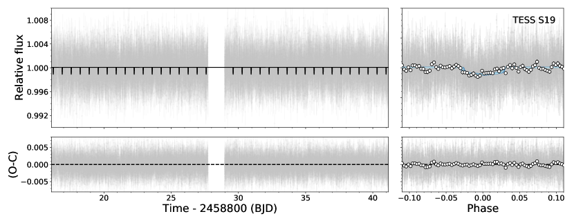
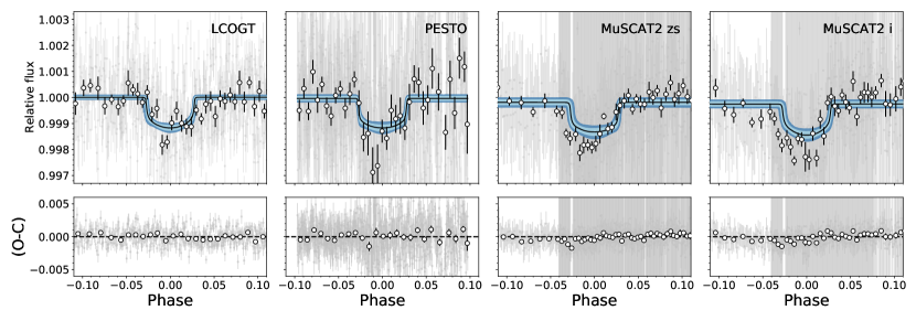
Figure 1: TESS and ground-based light curves of TOI-1685. Upper panels: PDC simple aperture photometry (SAP) TESS light curve of TOI-1685 and the corresponding phase-folded light curve. Lower panels: Phase-folded light curves of LCOGT, PESTO, and MuSCAT2 in filters $i$ and $z_{s}$ of TOI-1685. For all phase-folded light curves the residuals are shown for the USP found in the system. White circles are binned data (shown only for reference; the data used to fit the model were the unbinned points). Black curves are the best-fit models, and light and dark blue areas are the 68 % and 95 % credibility bands, respectively. The different sizes of the MuSCAT2 error bars correspond to the two observing nights.

Several follow-up studies have suggested that USPs are usually formed in multi-planetary systems (Sanchis-Ojeda et al., 2014), where multi-body interactions could play an important role in tidal migration. Accurately measuring the masses and orbits of any additional planet in such systems would be helpful in discriminating between different USP origin scenarios. Thus, in order to understand the processes involved in the formation and evolution of these planets, high cadence photometry and radial velocity (RV) campaigns, able to detect multi-planetary systems, are needed. Because of their short periods, it is relatively easy to precisely measure the parameters of USPs, but it is important to also explore and constrain additional planetary signals in systems that host USPs.

Theory and empirical data have shown that the occurrence rate of small planets tends to increase around late-type stars (Bonfils et al., 2013; Dressing & Charbonneau, 2015; Mulders et al., 2015; Gaidos et al., 2016). The Kepler (Borucki et al., 2010; Borucki, 2016) and K2 (Howell et al., 2014) space missions uncovered only a few USPs around M dwarfs ($T_{\rm eff}\lesssim$ 4000 K), such as Kepler-42 c, Kepler-732 c, Kepler-32 b, K2-137 b, K2-22 b, and K2-147 b (Muirhead et al., 2012; Morton et al., 2016; Smith et al., 2018; Dressing et al., 2017; Hirano et al., 2018). However, during the first years of the Transiting Exoplanet Survey Satellite (TESS; Ricker et al., 2015) mission, the number of discoveries nearly doubled (LP 791-18 b, LHS 3844 b, GJ 1252 b, LTT 3780 b, and TOI-1634 b; Crossfield et al., 2019; Vanderspek et al., 2019; Shporer et al., 2020; Nowak et al., 2020; Hirano et al., 2021).

In this paper, we report a transiting USP and a potential non-transiting planet candidate around the nearby M3.0 dwarf TOI-1685. The USP, with a period of 0.669 d, was initially discovered as a transiting planet candidate in TESS data and is confirmed here using ground-based photometry and RV measurements. The outer non-transiting planet candidate has a longer period of about 9 d.

The paper is organized as follows. Section 2 presents the TESS and ground-based photometry, lucky imaging, and high-resolution spectroscopy of TOI-1685. Section 3 presents the properties of the host star, either newly derived or collected from the literature. In Sect. 4 we present our search for the rotational period of the star, RV modeling, and the joint analysis of all available data made to constrain the properties of the system. In Sect. 5 we discuss our results and in Sect. 6 present our conclusions.

2 Data

2.1 TESS photometry

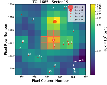
Figure 2: Target pixel files of TOI-1685 in TESS sector 19. The electron counts are color coded. The red bordered pixels are used in the SAP. The sizes of the red circles indicate the Gaia magnitudes of nearby sources down to $G$ = 18 mag and that of TOI-1685 (circle 1 marked with an $\times$).

TOI-1685 (TIC 28900646) was observed by TESS in 2 min short-cadence integrations during cycle 2 in sector 19 (see Table 1 for details) and was announced on 30 January 2020 as a TESS object of interest (TOI) through the dedicated TESS data public website from the Massachusetts Institute of Technology (MIT). We downloaded the data from the Mikulski Archive for Space Telescopes (MAST) using the lightkurve package (Lightkurve Collaboration et al., 2018). The photometric light curve was corrected for systematics (Pre-search Data Conditioning (PDC); Smith et al., 2012; Stumpe et al., 2012, 2014), which is optimized for TESS transit searches. The upper-left panel of Fig. 1 shows the PDC data for TESS sector 19 with our best-fit model (see Sect. 4.5 for details).

Table 1: TESS observations of TOI-1685.

Sector	Camera	CCD	Start date	End date
19	1	2	28 Nov. 2019	23 Dec. 2019

In order to search for any contaminant sources, we placed limits on the dilution factor of TOI-1685. We verified that the sources in the selection aperture in the TESS target pixel file (TPF) did not significantly affect the depth of the transits. The TPF created with tpfplotter (Aller et al., 2020) is shown in Fig. 2. Within the TPF aperture, we found only one extra source (TIC-28900668, Gaia EDR3 252366613254979328), which is separated by 15.6 arcsec from TOI-1685 and is 3.3 mag fainter. Further information comes from the TOI-1685 Gaia Early Data Release 3 (EDR3) renormalized unit weight error (RUWE) value (Lindegren et al., 2020) that is associated with each Gaia source. This is 1.18, below the critical value of 1.40 that indicates that the source may be non-single or otherwise problematic for the astrometric solution. We estimated the TESS minimum dilution factor at $D\sim 0.97$ from Eq. 6 in Espinoza et al. (2019). Since the PDC light curves are already corrected for possible nearby flux contamination, we fixed this value to 1.0 for all of our model fits presented in the following sections.

2.2 High-resolution imaging

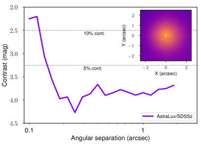
Figure 3: Sensitivity curve for the AstraLux high-spatial-resolution observation of TOI-1685 in the SDSS $z^{\prime}$ filter. The inset figure shows the AstraLux image when using the best 10 % of frames from the whole data cube.

Given the intrinsic faintness of M dwarfs and the large photometric apertures of wide-field surveys ($\sim$21 arcsec for TESS), the presence of an unresolved companion must be excluded before a planet candidate is confirmed. In some cases, other bright stars in the aperture mask can directly affect the photometry. To confirm the identification of the host star and to take nearby potential contaminants into account, we obtained seeing-limited and high-spatial-resolution imaging. We also needed to rule out the possibility that the transit in the light curve is due to an eclipsing binary. For this reason, we obtained ground-based photometry.

To search for companions at subarcsecond separations, we observed TOI-1685 with the lucky imaging instrument AstraLux (Hormuth et al., 2008) mounted on the 2.2 m telescope at the Observatorio de Calar Alto in Almería, Spain. We observed TOI-1685 on 25 February 2020 under good weather conditions with a mean seeing of 1.2 arcsec and at airmass 1.1. The instrument performs imaging with a fast readout (below the coherence time), creating data cubes of thousands of short-exposure frames. Those with the highest Strehl ratio (Strehl, 1902) are subsequently selected and combined into a final high-spatial-resolution image, which is done by the observatory pipeline (Hormuth et al., 2008). We observed in the Sloan Digital Sky Survey (SDSS) $z^{\prime}$ filter and obtained 87 600 frames with 20 ms exposure times and a field of view windowed to $6\times 6$ arcsec. Only the best 10 % of the frames were aligned and stacked. The final image is shown in the inset panel of Fig. 3. Based on this final image, we computed the sensitivity curve using the astrasens package with the procedure described by Lillo-Box et al. (2012, 2014). We found no evidence of additional sources within a 2 $\times$ 2 arsec² field of view and within the computed sensitivity limits, as shown in Fig. 3. This allowed us to set an upper limit to the contamination in the light curve of around 10 % down to 0.1 arcsec.

We further used this contrast curve to estimate the probability of contamination from blended sources in the TESS aperture that are undetectable in the public images. This probability is called blended source confidence (BSC), and the steps for estimating it were described by Lillo-Box et al. (2014). We used a python implementation of this approach (bsc) that uses the trilegal Galactic model (v1.6; Girardi et al., 2012) to retrieve a simulated source population of the region around the corresponding target. This is done in python with the astrobase implementation by (Bhatti et al., 2020). This simulation is used to compute the density of stars around a target position (within a radius of $\rho$ = 1 deg) and derive the probability of a chance alignment at a given contrast magnitude and separation. We used the default parameters for the bulge, halo, and disk (thin and thick), as well as the log-normal initial mass function from Chabrier (2001). We applied this technique to TOI-1685. Given the transit depth of planet TOI-1685 b, this signal could be mimicked by blended eclipsing binaries with magnitude contrasts of up to $\Delta m_{\rm b,max}=7.5$ mag in the SDSS $z^{\prime}$ bandpass. However, the high-spatial-resolution images provided a low probability of 1.5 % for an undetected source with such a magnitude contrast. The probability of this source being an appropriate eclipsing binary is well below 0.1 %. Given these numbers, we further assumed that the transit signal is not due to a blended binary star and that the probability of a contaminating source is very low.

2.3 Ground-based seeing-limited photometry

Table 2: Ground-based transit follow-up observations of TOI-1685.

Instrument	Country	Date	Filter	Exposure	Durationa	$N_{\rm obs}$	rmsb
				[s]	[min]		[ppt]
LCOGT	USA	26 August 2020	${I}$	50	173	123	1.29
		07 November 2020	${i_{\mathrm{p}}}$	25	266	270	1.47
		11 November 2020	${i_{\mathrm{p}}}$	50	279	199	1.01
PESTO	Canada	08 March 2020	${i^{\prime}}$	15	187	724	2.63
MuSCAT2	Spain	19 January 2020	${z_{\mathrm{s}}}$	15	179	328	1.24
			${i^{\prime}}$	15	179	238	1.18
		29 January 2020	${z_{\mathrm{s}}}$	15	331	333	1.70
			${i^{\prime}}$	15	331	333	1.71
LCOGTc	Spain, USA	22–31 December 2020	${V}$	100	39.83 [d]	20	13.7

One partial and one full transit of the red dwarf TOI-1685 were observed on 19 and 29 January 2021 with the MuSCAT2 instrument (Narita et al., 2019) at the 1.52 m Telescopio Carlos Sánchez at Observatorio del Teide, Spain. MuSCAT2 is a four-channel imager that performs simultaneous photometry in the $g^{\prime}$, $r^{\prime}$, $i^{\prime}$, and $z_{\mathrm{s}}$ bands. However, the low-quality $g^{\prime}$ and $r^{\prime}$ data were discarded from the analysis. The exposure times of our observations were 15 s in each band, and the observations were repeated for at least three times the USP period. Data reduction and photometric analysis were carried out using the custom-built pipeline for MuSCAT2 (Parviainen et al., 2020). The pipeline provides aperture photometry for a set of comparison stars and different aperture sizes. From them, the final light curves are chosen after a global optimization that takes into account the transit model and several different sources of systematics from covariates. The data obtained on 19 January 2021 were significantly affected by poor weather.

Four additional transit observations of TOI-1685 were taken with the Las Cumbres Observatory Global Telescope (LCOGT), on the night of 26 August 2020 and the nights of 7, 9, and 11 November 2020. The night of 9 November was discarded due to the bad quality of the data. Observations were taken with the 1.0 m telescopes at McDonald Observatory, USA, which were equipped with 4096 $\times$ 4096 pixel SINISTRO cameras, using the $I$ filter on the night in August and the $i_{p}$ filter on all the nights in November. Exposure times were set to 25, 50, and 50 s for the nights of 7 November, 11 November, and 26 August, respectively. Data reduction and photometric analysis were performed with the dedicated LCOGT banzai pipeline and AstroImageJ, respectively (Collins et al., 2017).

Finally, another full transit of TOI-1685 was observed at Observatoire du Mont-Mégantic, Canada, on 8 March 2020. Using the 1.6 m telescope equipped with the PESTO camera, the data were obtained in the $i^{\prime}$ filter with a 15 s exposure time. The bias subtraction, flat field division, and light curve extraction were also carried out using AstroImageJ.

Table 2 summarizes the three data sets, including the root mean square (rms) of the light curve fluxes. The resulting transit light curves obtained with MuSCAT2 (in $i$ and $z_{\mathrm{s}}$), LCOGT, and PESTO are shown in the bottom panels of Fig. 1.

2.4 CARMENES RV measurements

Table 3: Stellar parameters of TOI-1685.

Parameter	Value	Reference
Name and identifiers
Name	2MASS J04342248+4302148	2MASS
Karmna	J04343+430	AF15
TOI	1685	ExoFOP-TESS
TIC	28900646	Sta18
Coordinates and spectral type
$\alpha$ (J2000)b	04:34:22.55	Gaia EDR3
$\delta$ (J2000)b	+43:02:13.3	Gaia EDR3
Sp. type	M3.0 V	Terr15
$G$ [mag]	$12.284\pm 2.452$	Gaia EDR3
$T$ [mag]	$11.111\pm 0.007$	Sta19
$J$ [mag]	$9.616\pm 0.018$	2MASS
Parallax and kinematics
$V_{r}$ [$\mathrm{km\,s^{-1}}]$	$-43.4\pm 8.5$	Terr15
$\varpi$ [mas]	$26.589\pm 0.019$	Gaia EDR3
$d$ [pc]	$37.609\pm 0.027$	Gaia EDR3
$\mu_{\alpha}\cos\delta$ [$\mathrm{mas\,a^{-1}}$]	$+37.762\pm 0.022$	Gaia EDR3
$\mu_{\delta}$ [$\mathrm{mas\,a^{-1}}$]	$-87.062\pm 0.047$	Gaia EDR3
$U$ [$\mathrm{km\,s^{-1}}$]	$+35.6\pm 8.0$	This work
$V$ [$\mathrm{km\,s^{-1}}$]	$-29.8\pm 2.9$	This work
$W$ [$\mathrm{km\,s^{-1}}$]	$-3.14\pm 0.47$	This work
Gal. population	Thin disk	This work
Photospheric parameters
$T_{\mathrm{eff}}$ [K]	$3434\pm 51$	This work
$\log g$	$4.85\pm 0.04$	This work
[Fe/H]	$-0.13\pm 0.16$	This work
$v\sin i_{\star}$ [$\mathrm{km\,s^{-1}}$]	$<2.0$	This work
Physical parameters
$L_{\star}$ [$L_{\odot}$]	$0.0303\pm 0.0005$	This work
$M_{\star}$ [$M_{\odot}$]	$0.495\pm 0.019$	This work
$R_{\star}$ [$R_{\odot}$]	$0.492\pm 0.015$	This work
Activity and age
pEW(H$\alpha$) [Å]	$+0.51\pm 0.06$	This work
Age (Ga)	0.6–2.0	This work

2MASS: Skrutskie et al. (2006); AF15: Alonso-Floriano et al. (2015); ExoFOP-TESS: https://exofop.ipac.caltech.edu/tess/; Gaia EDR3: Gaia Collaboration et al. (2020); Sta18: Stassun et al. (2018); Terr15: Terrien et al. (2015); Sta19: Stassun et al. (2019).

TOI-1685 was observed 55 times with CARMENES between 8 August 2020 and 9 November 2020. CARMENES (Quirrenbach et al., 2014, 2018) is a high-resolution spectrograph installed at the 3.5 m telescope at the Observatorio de Calar Alto, Spain. It splits the incoming light into two beams that feed the visual (VIS; $0.52$–$0.96\text{\,}\mathrm{\SIUnitSymbolMicro m}$, $\mathcal{R}=94\,600$) and near-infrared (NIR; $0.96$–$1.71\text{\,}\mathrm{\SIUnitSymbolMicro m}$, $\mathcal{R}=80\,400$) channels via optical fibers. Exposure times ranged between about 1300 s (limited to the time needed to achieve a signal-to-noise ratio of 150, based on information from real-time exposure meters) and 1800 s (the maximum exposure time). We followed the standard data flow of the CARMENES guaranteed time observations (Caballero et al., 2016). In particular, we reduced the spectra with caracal (Zechmeister et al., 2014) and determined the corresponding RVs and spectral activity indices (see Sect. 4.3) with serval (Zechmeister et al., 2018). The RVs were corrected for barycentric motion, instrumental drift, secular acceleration, and nightly zero points (see Kaminski et al. 2018, Tal-Or et al. 2019, and, especially, Trifonov et al. 2020 for details).

The RVs, activity indices, and their corresponding uncertainties are listed in Table 7.

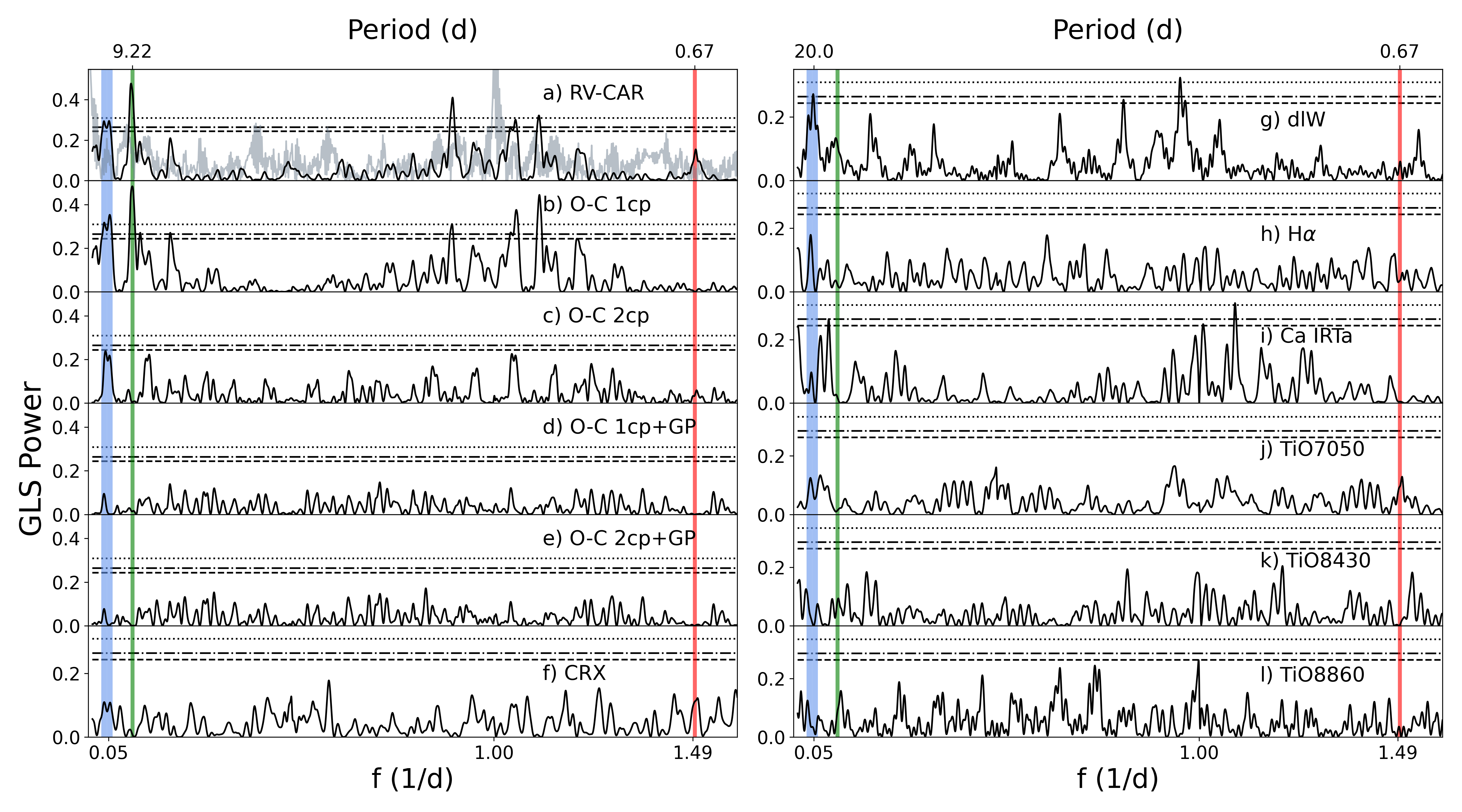
Figure 4: GLS periodograms of: ($a$) RVs from CARMENES VIS and the respective spectral window function (gray), ($b$) RV residuals after subtracting the one-planet signal, ($c$) RV residuals after subtracting the two-planet signal, ($d$) RV residuals after subtracting the one-planet signal plus GP, ($e$) RV residuals after subtracting the two-planet signal plus GP, ($f$-$l$) CRX, dLW, H$\alpha$, Ca IRTa (“a” corresponds to the Ca ii $\lambda$8498.0 Å line), TiO7050, TiO8430, and TiO8860 activity indices from CARMENES VIS data. The “cp” in the residual models (panels $a$-$e$) corresponds to circular orbits (for a detailed explanation, see Sect. 4.3). In all panels the vertical lines indicate the periods of 0.67 d (red, USP) and $\sim$9 d (green, second planet candidate). The rotational period of the star (blue line) falls in the region between $\sim$19 and 26 d. The horizontal lines mark the theoretical FAP levels of 1 % (dotted), 5 % (dash-dotted), and 10 % (dashed).

3 Stellar properties

The star TOI-1685 (2MASS J04342248+4302148, $V\approx$ 13.3 mag) is a nearby M3.0 V star at a distance of approximately 37.6 pc (Bailer-Jones et al., 2020). It has only been tabulated by a few proper-motion surveys (Lépine & Gaidos, 2011; Frith et al., 2013; Terrien et al., 2015). In this work, we recalculated all stellar parameters for this M dwarf. In particular, we measured $T_{\rm eff}$, surface gravity $\log{g}$, and iron abundance [Fe/H] from the stacked CARMENES VIS spectra by fitting them with a grid of PHOENIX-SESAM models, as in Passegger et al. (2019), the rotational velocity $v\sin{i}$ with the cross-correlation method, as in Reiners et al. (2018), and the stellar luminosity, $L_{\star}$, as in Cifuentes et al. (2020). The stellar radius, $R_{\star}$, was determined through the Stefan–Boltzmann law, $L_{\star}=4\pi R{{}_{\star}}^{2}\sigma T_{\rm eff}^{4}$, and the stellar mass, $M_{\star}$, using the mass-radius relation derived from main-sequence eclipsing binaries by Schweitzer et al. (2019). In particular, we used astro-photometry from Gaia EDR3 and photometry from Fourth U.S. Naval Observatory CCD Astrograph Catalog (UCAC4), Two Micron All Sky Survey (2MASS), and All Wide-field Infrared (AllWISE) (Zacharias et al., 2012; Skrutskie et al., 2006; Cutri et al., 2021).

We measured the pseudo-equivalent width, pEW(H$\alpha$), a key indicator of stellar activity, on the CARMENES stacked spectrum following Schöfer et al. (2019). In Sect. 4.1 we report the search for periodic signals in this and other spectroscopic activity indicators. As described in Sect. 4.2, we found that TOI-1685 has a rotation period of around 19 d. Although the star is rotating moderately fast for an early M dwarf, and the Galactic velocities $UVW$ indicate that it belongs to the relatively young thin disk (see Table 3), it is not associated with any particular young stellar kinematic group. The absence of X-ray emission in ROSAT observations (First ROSAT X-ray Survey (1RXS) ; Voges et al., 1999) and ultraviolet emission in the Galaxy Evolution Explorer (GALEX) images (Bianchi et al., 2017) is also an indication that the star is not very young. Using the gyrochronology relations from Barnes (2007) and Angus et al. (2015), and comparing the rotation period of the star with those of members in open clusters such as Praesepe (Rebull et al., 2017), we estimated an age of 0.6–2 Ga for the system.

Table 3 summarizes the stellar properties of TOI-1685, providing average values, uncertainties, and the corresponding references.

4 Analysis and results

4.1 Periodogram analysis of the RV data

We explored the generalized Lomb-Scargle (GLS) periodograms (Zechmeister & Kürster, 2009) of the RVs of TOI-1685. The periodogram and window function are shown in panel $a$ of Fig. 4. The strongest signal was found at about 9 d, with a nominal false alarm probability (FAP) $<$ 1 %, and its aliases around periods of 1 d (due to the sampling of the data). A double peak is visible in the period range of about 19–26 d with FAP $<$ 5 %, while a small isolated peak is discernible at the orbital frequency of TOI-1685 b. The formal FAP for this feature is $\gtrsim$ 10 %. However, we need to distinguish between an FAP for a peak anywhere in the frequency range of the periodogram and one at a known frequency in the data. Usually, the FAP is computed by finding the probability that noise creates a peak in the periodogram higher than what is observed over a wide frequency range, typically taken from near zero out to the Nyquist frequency. However, in this case there is a signal at the known orbital frequency of the planet, $f_{b}$. We need to assess the probability that random data produce more power than what is observed exactly at this frequency.

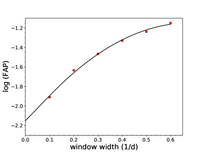
Figure 5: FAP versus window size using a bootstrap as described in Sect. 4.1. Red points are from the bootstrap, and the solid black line is the fit.

A better estimate of the FAP comes from using the bootstrap randomization method. Therefore, we randomly shuffled the RV values while keeping the time stamps fixed and noted how often a peak had a power higher than what was observed. However, this must be done over a narrow frequency range centered on $f_{b}$, which can be problematic. Too large a window and the FAP is over-estimated, too narrow and the results may not be statistically significant. As a result, we employed a ”windowing” bootstrap method (Hatzes, 2019) to compute the FAP over a wide frequency window centered on $f_{b}$ and then successively narrowed the window for additional bootstraps. The fit of the FAP versus window size, extrapolated to zero window length, yields the FAP at $f_{b}$. This method yielded an FAP $\approx$ 0.007, based on 100 000 bootstraps, as shown in Fig. 5. This fit confirms that the FAP of the peak at the orbital frequency of the transiting planet is less than 1 %.

4.2 Searching for the rotation period

In order to understand the origin of the $\sim$9 d and the double-peak ($\sim$19–26 d) signals present in the RV data, we searched for additional information in the periodograms of the activity indicators that serval provides, which are shown in panels $f$–$i$ of Fig. 4. These indicators comprise the chromatic index (CRX), differential line width (dLW), H$\alpha$ line emission, and Ca II infrared triplet (Ca IRT) emission. The titanium oxide indices that quantify the strengths of the TiO $\gamma$, $\epsilon$, and $\delta$ absorption band heads at 7050 Å, 8430 Å, and 8860 Å were derived from the individual CARMENES spectra following (Zechmeister et al., 2018; Schöfer et al., 2019) and are shown in panels $j$, $k$, and $l$, respectively. The double-peak signal visible in the RV periodogram is also strong in dLW ($\approx$20 d; panel $g$), which may indicate that this signal is related to stellar activity (Zechmeister et al., 2018).

As expected for an early-type M dwarf, the TiO7050, TiO8430, and TiO8860 indices, usually used to measure the properties of cool starspots of magnetically active stars, do not show significant signals. A measured median pEW(H$\alpha$) of +0.51 Å  classifies TOI-1685 as an H$\alpha$ inactive star (Jeffers et al., 2018). This is consistent with its low $v\sin i_{\star}$ value of $<$ 2.0 km$\rm s^{-1}$. The activity indices and their uncertainties are listed in Table 7.

In order to explore the stability of the double-peak signal, we computed the stacked-Bayesian GLS (s-BGLS) periodogram of the RV data with the normalization from Mortier & Collier Cameron (2017). The main idea was to stack the RV periodograms by subsequently adding observations and recalculating the periodogram. Figure 6 shows an s-BGLS periodogram between 0.5–40 d, after subtracting the USP signal. The signal at $\sim$9 d shows a first probability maximum after around 44 observations, after which the probability monotonically increases, as is expected for a Keplerian signal. On the other hand, the s-BGLS of the double-peak signal (centered around $\sim$19 d) shows a first probability maximum after around 44 measurements and then decreases for some time. This incoherence is characteristic for a non-planetary origin of the signal, and due to the evidence from the dLW we attributed it to the stellar rotation.

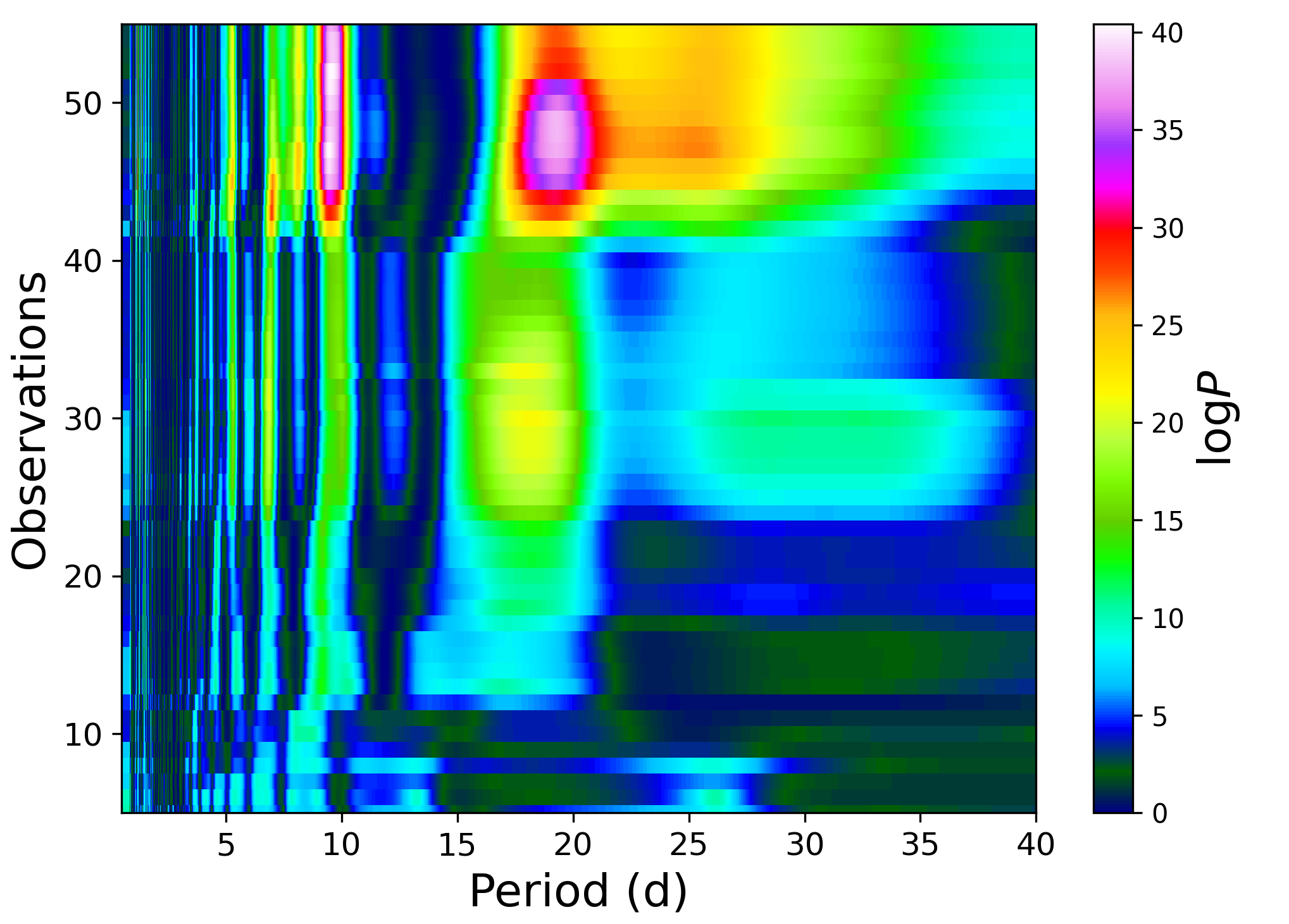
Figure 6: Evolution of the s-BGLS periodogram of the RV data between 0.5 d and 40 d, after subtracting the USP signal. The planet candidate is at $\sim$9 d, and the activity signal related to the rotational period is visible around 19 d. The number of data points included in the computation of the periodogram increases from bottom to top.

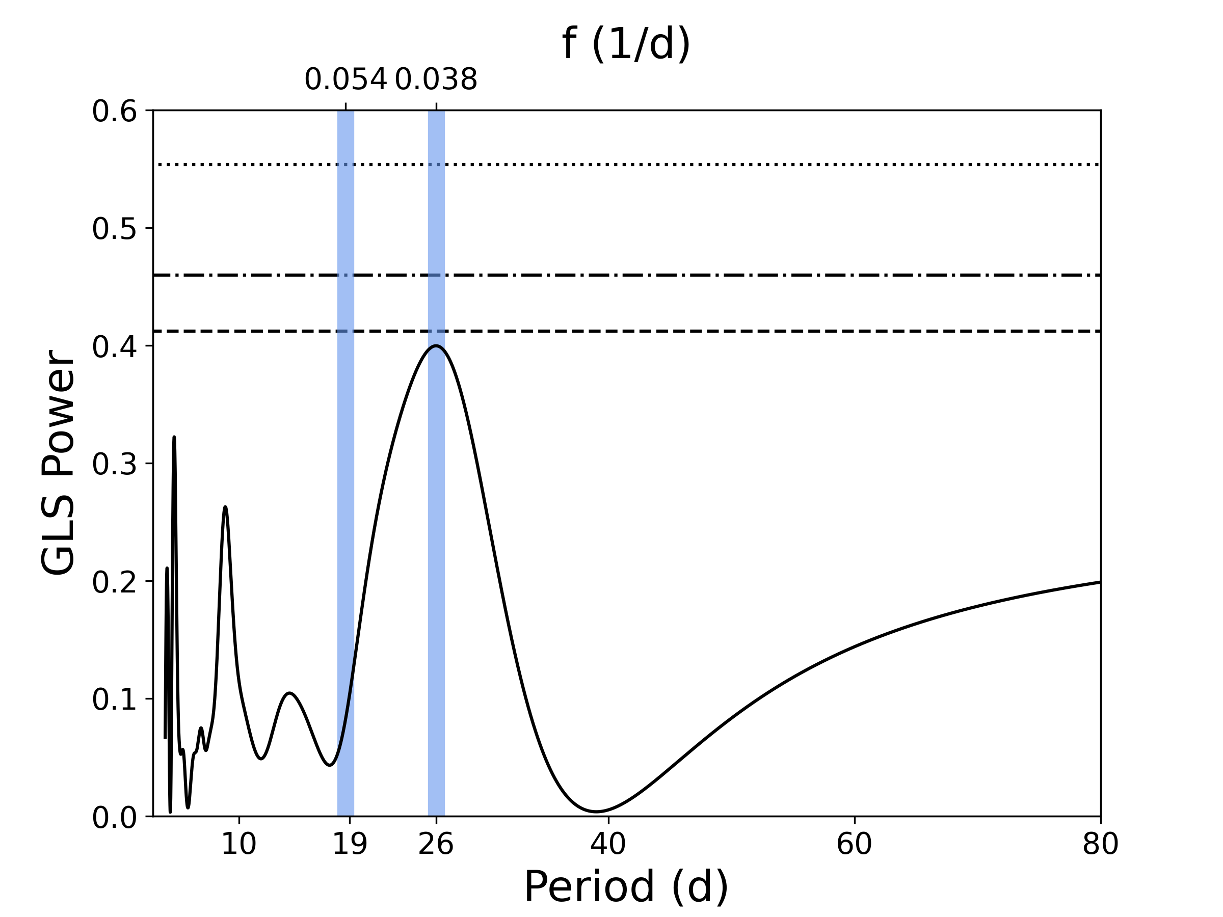
Figure 7: GLS periodogram of the joint $V$-band LCOGT Teide and Haleakalā light curve. The horizontal lines mark the theoretical FAP levels of 1 % (dotted), 5 % (dash-dotted), and 10 % (dashed). The highest peak, near the 10 % FAP level, which is related to the rotational period and has a period of $26.0\pm 2.5$ d, and the signal found in the RV data at $\sim$19 d are marked with blue vertical bands.

Additionally, we observed TOI-1685 in the $V$ band with the 40 cm telescopes of LCOGT at the Teide and Haleakalā observatories. The 40 cm telescopes are equipped with 3k $\times$ 2k Santa Barbara Instrument Group Charge-coupled device (SBIG CCD) cameras. with identical pixel scales of 0.571 arcsec and fields of view of 29.2$\times$19.5 arcmin. Weather conditions at both observatories were mostly clear, and the average seeing varied from 2.0 arcsec to 4.0 arcsec (for observation details, see Table 2). Raw data were processed with the banzai pipeline, which includes bad pixel, bias, dark, and flat-field corrections for each individual night. We performed aperture photometry for TOI-1685 and three reference stars of the field and obtained the relative differential photometry between the target and reference stars. We adopted an aperture of 16 pixels (9.1 arcsec), which minimizes the dispersion of the differential light curve. Figure 7 shows the GLS periodogram of the joint LCOGT Teide and Haleakalā photometric data. The highest peak close to the 10 % FAP level has a period of $26.0\pm 2.5$ d, which supports the notion that this signal is related to stellar activity and is consistent with the double peak at $\sim$19–26 d found in the spectroscopic data.

Finally, we searched for available photometric data for TOI-1685. We found some data in the All-Sky Automated Survey for SuperNovae light curves (ASAS-SN; Shappee et al., 2014; Kochanek et al., 2017), but unfortunately they were not useful for confirming the rotational period of TOI-1685.

4.3 Modeling results

To model the RV data, we used juliet(Espinoza et al., 2019), which allows fitting the data at a given prior volume. juliet searches the global posterior maximum based on the evaluation of the Bayesian log-evidence ($\ln{\mathcal{Z}}$), with which one can perform formal model comparisons given the differences in $\Delta\ln{\mathcal{Z}}$. To select our final model we used the criteria described in Trotta (2008), which consider a difference of $\Delta\ln{\mathcal{Z}}>5.0$ between models as ”significant” and of $\Delta\ln{\mathcal{Z}}>2.5$ at ”moderate,” favoring the former over the latter. Models with $\Delta\ln{\mathcal{Z}}<2$ are indistinguishable, which means none of them are preferred over the others.

juliet calculates the log-evidence via nested sampling algorithms. For the joint fit (see Sect. 4.5 for details) we used dynesty (Speagle, 2019) , and for the RV modeling we used MultiNest (Feroz et al., 2009), which employs the PyMultiNest package (Buchner et al., 2014). To model Keplerian RV signals we used radvel (Fulton et al., 2018), and for the Gaussian process (GP) modeling we used george (Ambikasaran et al., 2015). For the GP, we selected an exp-sin-squared kernel multiplied by a squared-exponential kernel, also known as the quasi-periodic (QP) kernel, which has the following form:

$$k(\tau)=\sigma_{\rm GP}^{2}\leavevmode\nobreak\ \exp\left(-\alpha_{\rm GP}\tau^{2}-\Gamma\sin^{2}({\pi\tau}{P_{\textnormal{rot}}})\right)\quad,$$ (1)

where $\sigma_{\rm GP}$ is the amplitude of the GP given in m$\rm s^{-1}$, $\Gamma$ is the amplitude of the GP sine-squared component, $\alpha$ is the square of the inverse length scale of the exponential component of the GP given in $\rm d^{-2}$, $\tau$ is the time lag in days, and $P_{\rm rot}$ is the period of the GP-QP component given in days. The GP-QP is a kernel that is widely used to model stellar activity signatures (see, e.g., Faria, 2017; Nava et al., 2020; Stock et al., 2020b; Kemmer et al., 2020; Bluhm et al., 2020, and references therein). The advantage of using a multiplied kernel is due to its exp-sine-squared factor, which enables the modeling of complex periodic signals. At the same time, the square-exponential factor allows changes in the periodic function over time, that is, either decreasing or increasing its amplitude. This combination is suitable for describing stochastic physical processes occurring in stars, such as the exponential growth or decay of active regions.

Table 4: RV model selection.

Models	Periods	$\ln{\mathcal{Z}}$	$\Delta\ln{\mathcal{Z}}$
1cp	0.67	–186.609 $\pm$ 0.107	0.0
1cp+GP	0.67	–177.843 $\pm$ 0.014	8.77
2cp	0.67, 9.22	–177.872 $\pm$ 0.073	8.74
1cp+1kp	0.67, 9.31	–178.501 $\pm$ 0.076	8.11
2cp+GP	0.67, 9.03	–176.609 $\pm$ 0.062	10.00
1cp+1kp+GP	0.67, 9.02	–175.149 $\pm$ 0.015	11.47
3cp	0.67, 9.12, 19.83	–175.464 $\pm$ 0.032	11.15
1cp+1kp+1cp	0.67, 9.01, 19.94	–174.369 $\pm$ 0.042	12.24
1cp+1kp+1kp	0.67, 9.00, 20.27	–174.791 $\pm$ 0.011	11.82

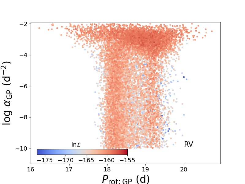
Figure 8: Posterior distribution of the GP fit to the RV data in the $\alpha$ versus $\rm P_{rot}$ plane for TOI-1685. The color coding shows the log-likelihood normalized to the highest value in the posterior sample.

4.4 Only RV data

We performed an extensive model comparison on the RV data to find the model that accounts best for all three signals described in Sect. 4.2. As we discussed, the $\sim$9 d signal does not seem to be related to the $\sim$19 d rotational period of TOI-1685; it could be due to a second (non-transiting) planet in the system. An overview of the different models and their Bayesian evidence is shown in Table  4. The residual periodograms for the best log-evidence are shown in Fig. 4.

Since the USP signal was statistically significant (see Sect. 4.1 for details), we started fitting the RVs with a one-planet circular model around the USP period using uniform priors between 0.6 d and 0.7 d. The residual periodogram is shown in panel $b$ of Fig. 4. Here, the strongest periodicity is at 9.22 d (FAP $<$ 1 %). After subtracting the USP period and the 9.22 d signal (using uniform priors between 8 d and 10 d) with a circular two-planet fit, only the double-peak signal at $P\approx$ 19–26 d with FAP $\sim$ 10 % remained (panel $c$). The double-peak structure and the activity indicators described in Sect. 4.2 show that the $\sim$19–26   signal could be related to the stellar rotation period. Therefore, we next investigated whether including a GP to account for this signal improved the log-evidence of the fit.

We did our GP prior selection and final prior volume definition as described by Stock et al. (2020a). We started by using a wide prior for the GP period and GP $\alpha$ values. We constructed a GP $\alpha$-period diagram, which is useful for identifying whether stronger correlated noise (small $\alpha$) favors a certain periodicity (see, e.g., Stock et al., 2020b, and references therein). With this first approach, the diagram showed a plateau along with all periods in the range $\log{\alpha}\gtrsim$ –2 as well as a structure around the $\sim$19 d signal. The origin of the plateau is that the GP is essentially modeling white noise at that $\alpha$ range. As we were mostly interested in fitting the spectral region around the suspected stellar rotational period with the GP, we set narrow uniform priors for the signal centered at $\sim$19 d, and we cut off the plateau by constraining the $\alpha$ values. Figure 8 shows a scatter plot of the sampled $\alpha$ values of the QP kernel over the sampled rotational periods using the priors presented in Table 8. Considering this plane, we inferred that the likelihood and number of posterior samples around $\sim$19 d are consistent with a periodic signal present over the entire time of observations.

Once the parameters of our GP-QP were chosen, we performed a simultaneous fit to a one-planet circular model together with a GP (1cp+GP). As we expected, including a GP significantly improved the log-evidence compared to the one-planet circular fit alone ($\Delta\ln{\mathcal{Z}}\sim 8.8$). To account for the signal at $\sim$9 d, we further performed a two-planet plus GP model, where we either fixed the eccentricity (2cp+GP) or kept it free (1cp+1kp+GP). In these cases, the differences between these models with the 1cp+GP fit were $\Delta\ln{\mathcal{Z}}$ $\sim$1.2 for 2cp+GP and $\Delta\ln{\mathcal{Z}}$ $\sim$2.7 for 1cp+1kp+GP. In the first case, the difference made these two models indistinguishable from each other, while in the second the difference made the 1cp+1kp+GP fit moderately favored. On the other hand, the difference between them was $\Delta\ln{\mathcal{Z}}$ $\sim$1.5, which made the models indistinguishable if they were equally likely a priori, so the simplest model should be chosen in this case.

Additionally, we performed a three-planet model fit and compared the $\Delta\ln{\mathcal{Z}}$ with the 1cp+GP fit. In this case, we used uniform priors between 15 and 30 d, the suspected region for the stellar rotational period (Sect. 4.2). In all cases, the differences were $\Delta\ln{\mathcal{Z}}<5$, which implied that none of them were significantly favored. However, we noticed that most of the models that include three signals show a $\Delta\ln{\mathcal{Z}}\gtrsim 2.5$ compared to the 1cp+GP, which makes them moderately favored; hence, we cannot immediately rule out an additional signal in the system.

We decided to choose the 1cp+GP as our fiducial model, and in Sect. 5.2 we explore the possibility of include the $\sim$9 d signal with a 2cp+GP model. The residuals of these two fits are shown in panels $d$ and $e$ of Fig. 4, respectively, where no additional significant peaks are detectable.

4.5 Joint fit

Table 5: Posterior distributions of the juliet joint fit for the instrumental parameters.

Parametera	TOI-1685
Stellar parameters
$\rho_{\star}$ ($\mathrm{g\,cm\,^{-3}}$)	$5.797^{+0.064}_{-0.060}$
Photometry parameters
$M_{\mathrm{TESS,S19}}$ ($10^{-5}$)	$-7.63^{+1.60}_{-1.60}$
$\sigma_{\mathrm{TESS,S19}}$ (ppm)	$2.63^{+15.44}_{-2.26}$
$q_{1,\mathrm{TESS}}$	$0.37^{+0.27}_{-0.20}$
$q_{2,\mathrm{TESS}}$	$0.54^{+0.29}_{-0.32}$
$M_{\mathrm{LCOGT}}$ ($10^{-5}$)	$-0.46^{+4.31}_{-4.30}$
$\sigma_{\mathrm{LCOGT}}$ (ppm)	$826.79^{+44.54}_{-42.89}$
$q_{1,\mathrm{LCOGT}}$	$0.63^{+0.22}_{-0.29}$
$M_{\mathrm{PESTO}}$ ($10^{-5}$)	$3.41^{+7.36}_{-7.42}$
$\sigma_{\mathrm{PESTO}}$ (ppm)	$967.07^{+22.71}_{-40.25}$
$q_{1,\mathrm{PESTO}}$	$0.49^{+0.29}_{-0.29}$
$M_{\mathrm{MuSCAT2\leavevmode\nobreak\ i}}$ ($10^{-5}$)	$24.92^{+7.97}_{-7.97}$
$\sigma_{\mathrm{MuSCAT2\leavevmode\nobreak\ i}}$ (ppm)	$7.06^{+63.95}_{-6.49}$
$q_{1,\mathrm{MuSCAT2\leavevmode\nobreak\ i}}$	$0.71^{+0.20}_{-0.30}$
$M_{\mathrm{MuSCAT2\leavevmode\nobreak\ z_{s}}}$ ($10^{-5}$)	$18.75^{+8.84}_{-8.88}$
$\sigma_{\mathrm{MuSCAT2\leavevmode\nobreak\ z_{s}}}$ (ppm)	$5.17^{+48.83}_{-4.69}$
$q_{1,\mathrm{MuSCAT2\leavevmode\nobreak\ z_{s}}}$	$0.54^{+0.29}_{-0.32}$
RV parameters
$\gamma_{\mathrm{CARMENES}}$ ($\mathrm{m\,s^{-1}}$)	$0.34^{+2.69}_{-2.78}$
$\sigma_{\mathrm{CARMENES}}$ ($\mathrm{m\,s^{-1}}$)	$2.35^{+0.79}_{-0.93}$
GP hyperparameters
$\sigma_{\mathrm{GP,RV}}$ ($\mathrm{m\,s^{-1}}$)	$6.46^{+3.17}_{-1.68}$
$\alpha_{\mathrm{GP,RV}}$ ($10^{-3}\,\mathrm{d^{-2}}$)	$0.25^{+1.70}_{-0.25}$
$\Gamma_{\mathrm{GP,RV}}$	$5.76^{+2.75}_{-3.35}$
$P_{\mathrm{rot;GP,RV}}$ (d)	$18.66^{+0.71}_{-0.56}$

Table 6: Derived planetary parameters for TOI-1685 b and TOI-1685 [c].

Parameter	TOI-1685 b
Planet parameters
$P_{\rm b}$ (d)	$0.6691403^{+0.0000023}_{-0.0000021}$
$t_{0,b}{\rm}$ (BJD)	$2458816.22615^{+0.00059}_{-0.00060}$
$a_{\rm b}/R_{\star}$	$5.158^{+0.019}_{-0.018}$
$p=R_{\rm b}/R_{\star}$	$0.0317^{+0.0009}_{-0.0010}$
$b=(a_{\rm b}/R_{\star})\cos i_{\rm b}$	$0.473^{+0.048}_{-0.054}$
$i_{\rm b}$ (deg)	$84.74^{+0.60}_{-0.54}$
$r_{1}$	$0.65^{+0.03}_{-0.04}$
$r_{2}$	$0.0317^{+0.0009}_{-0.0010}$
$K_{\rm b}$ ($\mathrm{m\,s^{-1}}$)	$4.41^{+0.73}_{-0.73}$
Derived physical parameters
$M_{\rm b}$ ($M_{\oplus}$)	$3.78^{+0.63}_{-0.63}$
$R_{\rm b}$ ($R_{\oplus}$)	$1.70^{+0.07}_{-0.07}$
$\rho_{\rm b}$ (g cm-3)	$4.21^{+0.95}_{-0.82}$
$g_{\rm b}$ (m s-2)	$12.79^{+2.49}_{-2.28}$
$T_{\textnormal{eq,b}}$ (K)	$1069^{+16}_{-16}$
$S_{\rm b}$ ($S_{\oplus}$)	$217^{+13}_{-13}$
Parameter	TOI-1685 [c]c
$P_{\rm c}$ (d)	$9.025^{+0.104}_{-0.119}$
$t_{0,c}{\rm}$ (BJD)	$2458820.4^{+2.9}_{-2.6}$
$a_{\rm c}/R_{\star}$	$29.23^{+0.23}_{-0.24}$
$K_{\rm c}$ ($\mathrm{m\,s^{-1}}$)	$4.53^{+1.01}_{-1.02}$
$T_{\textnormal{eq,c}}$ (K)	$449.1^{+6.9}_{-6.9}$
$S_{\rm c}$ ($S_{\oplus}$)	$6.76^{+0.42}_{-0.41}$
$M_{\rm c}\rm sini$ ($M_{\oplus}$)	$9.21^{+2.06}_{-2.07}$

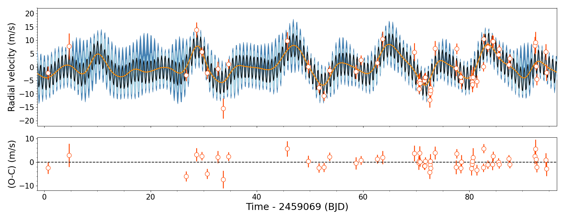
Figure 9: RV data from CARMENES (red). The gray curve is the median best-fit Keplerian juliet model, the light and dark blue areas are its 68 % and 95 % credibility bands, and the orange curve is the QP kernel (GP-QP).

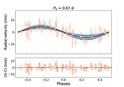
Figure 10: Phase-folded RV curves and their residuals of the USP. Black curves are the best-fit models, and blue areas are the 68 % and 95 % credibility bands.

In order to obtain precise parameters of the TOI-1685 system, we performed a joint analysis with juliet. For the joint fit we used TESS, LCOGT, PESTO, MuSCAT2, and CARMENES VIS data. For the transit modeling, juliet makes use of the batman package (Kreidberg, 2015). To parameterize the quadratic limb-darkening effect in the TESS photometry, we employed the efficient, uninformative sampling scheme of Kipping (2013) and a quadratic law. For LCOGT, PESTO, and MuSCAT2 photometry, we used a linear law to parameterize the limb-darkening effect. We followed the Espinoza (2018) parameterization to explore the full physically plausible parameter space for the planet-to-star radius ratio, $p=R_{\rm p}/R_{\star}$, and the impact parameter, $b$. The model selection was performed based on the analyses on the photometric data plus the highest peaks in the RV periodogram. As discussed in Sect. 4.3, we selected as our fiducial model one planet with a circular orbit and a QP GP for the stellar rotation (1cp+GP).

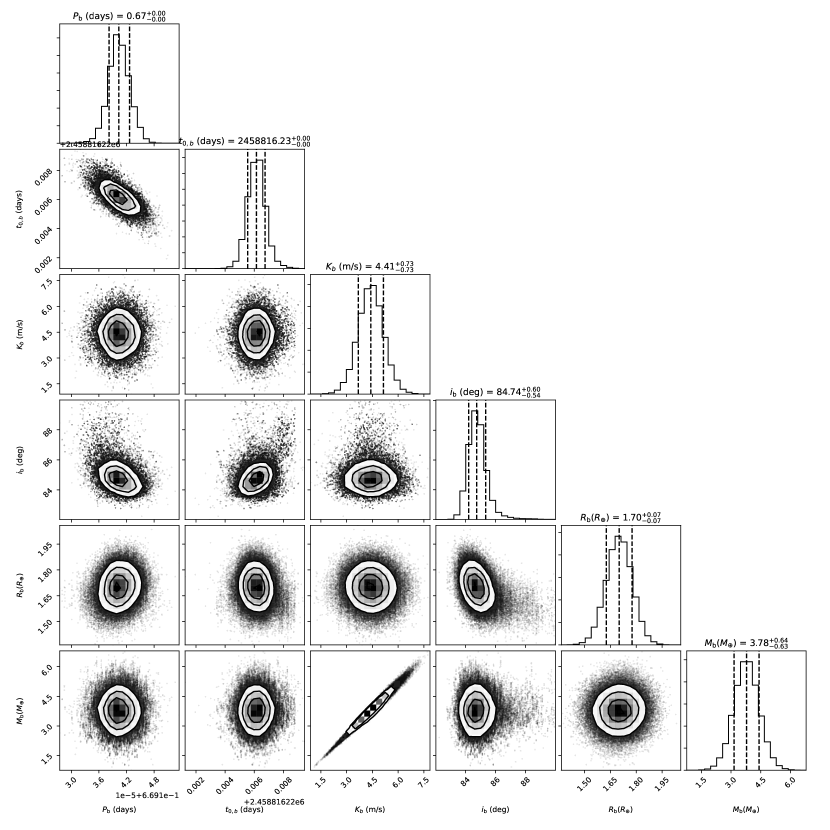
Figure 15: Posterior distribution for the joint model parameters (1cp+GP) derived with juliet.

The selected priors for our joint fit are presented in Table 8. The posterior distributions of our joint fit are presented in Tables 5 and 6, while the resulting photometry and RV models are presented in Figs. 1,  9, and  10, respectively. The obtained posterior probabilities are presented in Fig. 15. The maximum posterior of the rotational period of the GP periodic component was around 19 d, in agreement with the region at $\approx$ 19–26 d observed in the GLS RV periodogram (Fig. 4 and Sect. 4.2).

5 Discussion

5.1 Ultra-short-period planet: TOI-1685 b

We present the discovery of the USP TOI-1685 b, which orbits its host star with a period of 0.669 d. To confirm the planetary nature of the TESS transiting candidate, we obtained high-resolution spectra using the CARMENES spectrograph. We derived a mass of $M_{\rm b}$ = $3.78^{+0.63}_{-0.63}$ $M_{\oplus}$, a radius of $R_{\rm b}$ = $1.70^{+0.07}_{-0.07}$ $R_{\oplus}$, and a bulk density of $\rho_{\rm b}$ = $4.21^{+0.95}_{-0.82}$ g cm^-3 (see Table 6).

Figure 11 shows TOI-1685 b in the context of all known exoplanets from NASA’s exoplanet archive, with $R\leq$ 4 $R_{\oplus}$ and a planet bulk density of $\rho\leq$ 15 g cm^-3. Here, the USPs with orbital periods ranging from less than 10 hours to about one day tend to be smaller than 2 $R_{\oplus}$ (Winn et al., 2018) and are believed to have lost their atmospheres due to X-ray and ultraviolet (XUV) photo-evaporation from their host stars (e.g., Owen & Wu, 2013b; López & Fortney, 2013; Jin et al., 2014; Chen & Rogers, 2016; Owen & Wu, 2017). With an equilibrium temperature of $T_{\textnormal{eq}}$ = $1069\pm 16$ K, it is likely that TOI-1685 b has gone through a similar process. In terms of separation from its host star, TOI-1685 b is one of the closest known planets with a mass determination. An insolation flux of $S$ = $217\pm 13$ $S_{\oplus}$ also makes TOI-1685 b one of the hottest transiting super-Earth discovered to date. TOI-1685 b is the third known USP to be found orbiting an M star, and the least dense of the three.

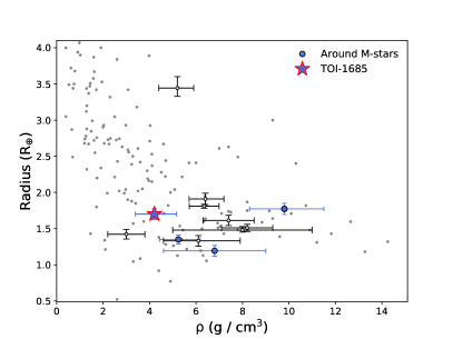
Figure 11: Density-radius diagram for all known exoplanets with planet bulk densities $\rho\leq$ 15 g cm^-3 and radii $R\leq$ 4 $R_{\oplus}$ (gray) from the NASA exoplanet archive. USPs are drawn in black and are shown with the error bars of the measurements. Blue-filled circles mark USPs around M dwarfs, and the filled star symbol is TOI-1685 b.

A comparison of the physical properties of TOI-1685 b with compositional models from Zeng et al. (2016, 2019) is shown in Fig. 12. The diagram reveals that TOI-1685 b is consistent with a bulk composition of 50 % H₂0 and 50 % silicate.

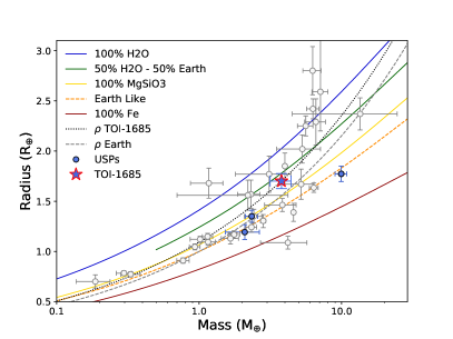
Figure 12: Mass-radius diagram in Earth units. Open circles are transiting planets around M-dwarf stars from the Transiting Extrasolar Planets Catalogue (TEPCat) database (Southworth 2011 and Martínez-Rodríguez et al. 2019), blue-filled circles are USPs, and the filled star symbol is TOI-1685 b.

Finally, the proximity of TOI-1685 b to its host star, and assuming that the planet has not lost its atmosphere, makes TOI-1685 b an attractive target for atmospheric characterization. In order to estimate the suitability of TOI-1685 b for such characterization, we calculated the spectroscopic metrics from Kempton et al. (2018). The transmission spectroscopy metric (TSM) and the emission spectroscopy metric (ESM) are analytic metrics for the expected S/N of transmission and emission spectroscopy observations by James Webb Space Telescope (JWST).

The TSM is estimated based on the strength of spectral features and the brightness of the host star, assuming a cloud-free atmosphere. The ESM is an approximation of the expected S/N for a single secondary eclipse observation integrated over the full 5–10 $\mu$m bandpass of the low-resolution spectroscopy (LRS) mode of the JWST Mid-Infrared Instrument (MIRI). We estimated the ESM of TOI-1685 b to be about 13.9. This is larger than that of Gl 1132 b, which is considered a benchmark rocky planet for emission spectroscopy (Kempton et al., 2018). The top panel of Fig. 13 shows the ESMs of exoplanets with measured masses, either through RVs or transit-timing variations (TTVs), with a radius from the NASA exoplanet archive of less than 3 $R_{\oplus}$. We chose this radius cutoff in order keep only the most likely terrestrial planets, and we excluded potential small sub-Neptunes (Kempton et al., 2018). Planets with ESMs on the order of or above the value of Gl 1132 b are separated from the others by a horizontal dotted line. TOI-1685 b is one of the hottest members of this family of small rocky planets suitable for emission spectroscopy.

We calculated a TSM value of 86$\pm$18 for TOI-1685 b. The TSMs of small exoplanets (1.5 $R_{\oplus}<R_{p}<3\,R_{\oplus}$) are shown in the bottom panel of Fig. 13. We excluded planets with radii smaller than 1.5 $R_{\oplus}$ from this panel to make the TSMs comparable, as defined in (Kempton et al., 2018). A favorable TSM value for this class of planets is around 90 or higher (Table 1 in Kempton et al., 2018). This implies that TOI-1685 b would be a suitable target for atmospheric characterization through transmission spectroscopy as well. The suitability of TOI-1685 b for both transmission and emission spectroscopy makes this planet a worthy target for atmospheric characterization over a wide orbital phase.

The equilibrium temperature of TOI-1685 b is estimated to be about 1070 K. This is larger than the 880 K temperature threshold above which planets are expected to have molten surfaces, such as 55 Cnc e (McArthur et al., 2004). No thick H₂-dominated primary atmosphere is expected at these high temperatures, except possibly an exosphere maintained by vaporized rocks (Mansfield et al., 2019) or a secondary outgassing atmosphere due to volcanic activity. If such a substantial exosphere exists, it could provide critical observable tracers to shed light on the planet formation and evolution of USPs as it would directly trace the surface or near-surface composition of these planets.

Following such a scenario, it is expected that small exoplanets at higher temperatures have higher bulk densities. This is indeed what has been observed so far, as shown by the red shaded region in Fig. 14. However, TOI-1685 b does not follow such a prediction. This may suggest that TOI-1685 b maintains a substantial atmosphere, unlike other hot small planets. In such a scenario, water, carbon dioxide, or methane features could be observable in its atmosphere (Molaverdikhani et al., 2019b, a) or such atmospheric features might be obscured by clouds (Molaverdikhani et al., 2020). Nevertheless, future emission and transmission spectroscopy of TOI-1685 b is needed to answer the question of whether the entire atmosphere has escaped or a substantial atmosphere has been maintained on TOI-1685 b, making this USP a rather unusual and interesting planet discovery.

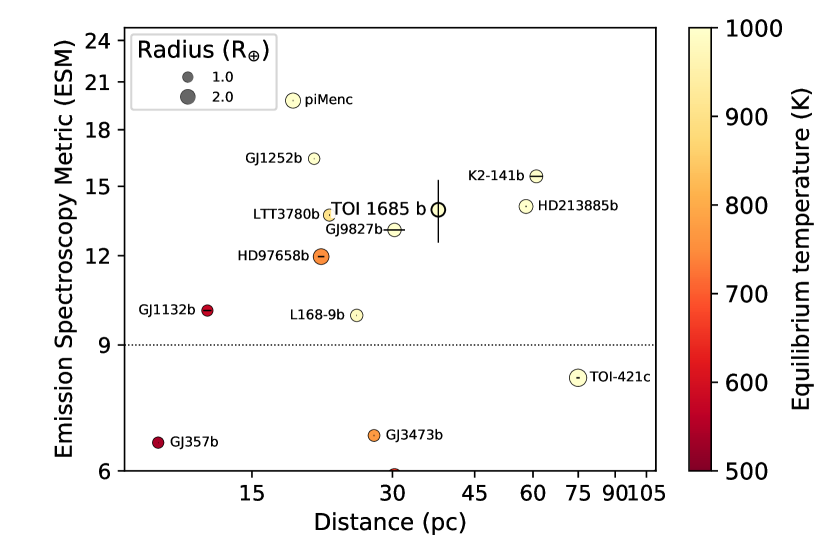
Figure 13: ESM and TSM metrics for TOI-1685 b. Top: ESM for exoplanets with a radius of less than 3 $R_{\oplus}$. Bottom: TSM for exoplanets with a radius of less than 3 $R_{\oplus}$ but larger than 1.5 $R_{\oplus}$. All planets have mass determination by either RVs or TTVs. TOI-1685 b is labeled and marked with a thicker black borderline in both panels. For most exoplanets, the error bars, in distance, are smaller than the symbol size. The uncertainties in the ESM and TSM are only plotted for TOI-1685 b.

Figure 14: Density-equilibrium temperature diagram of warm-hot exoplanets with a radius of less than 3 $R_{\oplus}$ around M dwarfs. All planets have mass determination by either RVs or TTVs. TOI-1685 b is labeled and marked with a thicker black borderline. Some densities are marked as reference by horizontal lines, including Earth (dashed orange), H₂O (blue), and 50 % H₂O, 50% silicate (green). The observed $\rho$-$T\rm_{eq}$ space before the discovery of TOI-1685 b is shaded in red to illustrate the dissimilarity of TOI-1685 b with previous discoveries.

5.2 The planet candidate TOI-1685 [c]

Our RV modeling shows moderate evidence for a second potentially planetary signal in the system. As discussed in Sect, 4.2, the observed period of $\sim 9$ d is not obviously linked to the stellar rotation period of $\sim$26 d, and the analysis of a comprehensive set of activity indicators revealed no signs of stellar activity at the period in question. However, the fact that the $\sim$9 d signal is close to the first harmonic of the likely rotational period derived from the RVs implies that we cannot be completely certain about its origin.

A comparison of the log-evidence values of the different models considered does not settle the issue as the differences between them are not highly significant. The situation is further complicated by the fact that sinusoidal or Keplerian models may also represent stellar activity well, especially over a relatively short time span.

Nevertheless, the significance and the coherence of the 9 d signal compared to the presumed stellar activity signal at 19 d does lend some support to a planetary origin. After all, it represents the highest peak in the RV periodogram (Fig. 4), and it seems to be the most persistent (Fig. 6). Under the assumption that the signal is indeed due to a planet, we performed a 2cp+GP model fit. We used the same distribution prior as that presented in Table 8, and for the signal at $\sim$ 9 d we used a uniform distribution between 8.5 and 9.5 d.

From our joint fit, we derived for the planet candidate a period of $P_{\rm c}$ = $9.03^{+0.10}_{-0.12}$ d and a minimum mass of $M_{\rm c}$ = $9.2^{+2.1}_{-2.1}$ $M_{\oplus}$; additional planet parameters are reported in Table 6. The obtained parameters with the 2cp+GP model were consistent within one sigma with those derived from the 1cp+GP model.

As a further test, we investigated whether the two-planet system would be dynamically stable. We used Exo-Striker (Trifonov, 2019) to check the long-term stability of planetary systems via the angular momentum deficit key parameter (Laskar & Petit, 2017). The best joint fit resulted in a stable solution for the TOI-1685 system.

6 Conclusion

We present the discovery of a possible multi-planetary system around the M3.0 V star TOI-1685. The system has one transiting planet with an ultra-short orbital period plus another planet candidate at a wider orbit found only in RV data. The USP TOI-1685 b was first detected in the photometric time series of sector 19 of the TESS mission. We collected CARMENES RV data, as well as photometric transit follow-up observations from LCOGT, PESTO, and MuSCAT2, with which we confirmed its planetary nature. From the joint analysis, we derived a mass of $M_{\rm b}$ = $3.78^{+0.63}_{-0.63}$ $M_{\oplus}$ and a radius of $R_{\rm b}$ = $1.70^{+0.07}_{-0.07}$ $R_{\oplus}$. The derived bulk density of $\rho_{\rm b}$ = $4.21^{+0.95}_{-0.82}$ g cm^-3 makes TOI-1685 b the least dense USP around an M dwarf known to date.

A comparison of the physical properties of TOI-1685 b with compositional models revealed a bulk composition of 50 % H₂0 and 50 % silicate. With a mass and radius precision better than 18 % and 5 %, respectively, TOI-1685 b complements the sample of well-characterized small planets orbiting nearby M dwarfs. Its proximity to its host star and the measured values for the TSM and the ESM metrics qualify this planet for atmospheric characterization through emission and transmission spectroscopy, as well as make it an interesting planet for studying atmospheric evolution and escape processes.

In the exploration of the RV data, a significant signal at $\sim$9 d was also found. To explore the origin of this signal, we analyzed the periodogram for RV activity indicators as well as the s-BGLS periodogram, and the signal was found to be persistent.

To model the stellar activity we used a GP-QP model based on a QP kernel plus two circular orbits (2cp+GP). However, due to the proximity of the $\sim$9 d planet candidate period to half of the stellar rotation period, we cannot rule out that it is related to stellar activity. Nevertheless, the strength and coherence of the signal make it a promising planet candidate. However, based on the currently available RV data, it is not possible to confidently claim the detection of a second planet in the system. To reach a solid conclusion, more data will be needed.

Appendix A Additional figures and tables

Table 7: RV measurements and spectroscopic activity indicators for TOI-1685 from CARMENES VIS spectra.

BJD	RV	CRX	dLW	H$\alpha$	Ca IRTa	TiO7050	TiO8430	TiO8860
(–2450000)	(m s-1)	(m s-1 Np-1)	(m2 s-2)
9069.6744	-1.87$\pm$2.43	9.17$\pm$24.55	23.23$\pm$3.44	0.8715$\pm$0.0043	0.6121$\pm$0.0031	0.616$\pm$0.002	0.836$\pm$0.004	0.004$\pm$0.003
9073.6703	8.05$\pm$4.91	30.68$\pm$50.73	23.22$\pm$5.48	0.8531$\pm$0.0095	0.6132$\pm$0.0067	0.620$\pm$0.004	0.822$\pm$0.008	0.008$\pm$0.006
9095.6713	-2.74$\pm$2.14	-3.32$\pm$19.66	4.05$\pm$2.91	0.8605$\pm$0.0037	0.6124$\pm$0.0029	0.616$\pm$0.002	0.831$\pm$0.003	0.003$\pm$0.003
9097.6749	14.20$\pm$2.81	12.22$\pm$28.42	-7.50$\pm$3.14	0.8794$\pm$0.0059	0.6111$\pm$0.0044	0.612$\pm$0.003	0.834$\pm$0.005	0.005$\pm$0.004
9098.6754	5.97$\pm$1.78	21.89$\pm$14.47	-1.50$\pm$2.17	0.8591$\pm$0.0029	0.6054$\pm$0.0023	0.619$\pm$0.001	0.838$\pm$0.003	0.003$\pm$0.002
9099.6693	-1.93$\pm$2.13	-23.05$\pm$20.72	0.91$\pm$2.25	0.8480$\pm$0.0031	0.6069$\pm$0.0025	0.616$\pm$0.001	0.840$\pm$0.003	0.003$\pm$0.002
9101.6859	-0.34$\pm$2.63	-20.53$\pm$24.23	1.27$\pm$3.41	0.8539$\pm$0.0050	0.6010$\pm$0.0037	0.616$\pm$0.002	0.835$\pm$0.004	0.004$\pm$0.004
9102.6845	-15.14$\pm$3.71	45.34$\pm$26.79	0.25$\pm$2.40	0.8520$\pm$0.0047	0.6002$\pm$0.0035	0.616$\pm$0.002	0.829$\pm$0.004	0.004$\pm$0.004
9103.6777	1.44$\pm$1.84	11.14$\pm$14.56	-2.91$\pm$1.79	0.8635$\pm$0.0030	0.6062$\pm$0.0024	0.619$\pm$0.001	0.840$\pm$0.003	0.003$\pm$0.002
9114.7106	10.09$\pm$3.26	-20.69$\pm$33.19	-10.15$\pm$3.45	0.8709$\pm$0.0058	0.6069$\pm$0.0042	0.618$\pm$0.002	0.841$\pm$0.005	0.005$\pm$0.004
9118.6966	0.46$\pm$2.46	83.69$\pm$15.50	0.61$\pm$2.41	0.8573$\pm$0.0040	0.6134$\pm$0.0031	0.617$\pm$0.002	0.832$\pm$0.003	0.003$\pm$0.003
9120.6746	-7.34$\pm$1.95	32.41$\pm$17.54	-4.17$\pm$1.82	0.8422$\pm$0.0030	0.6135$\pm$0.0024	0.617$\pm$0.001	0.834$\pm$0.003	0.003$\pm$0.002
9121.6352	-10.46$\pm$1.90	-24.59$\pm$17.06	-0.05$\pm$1.94	0.8777$\pm$0.0033	0.6192$\pm$0.0025	0.618$\pm$0.001	0.833$\pm$0.003	0.003$\pm$0.003
9122.6841	-0.98$\pm$1.82	25.19$\pm$17.66	-1.04$\pm$2.68	0.8602$\pm$0.0046	0.6126$\pm$0.0035	0.617$\pm$0.002	0.838$\pm$0.004	0.004$\pm$0.003
9127.6877	-1.46$\pm$2.61	-28.39$\pm$22.25	0.54$\pm$2.89	0.8678$\pm$0.0041	0.6235$\pm$0.0032	0.616$\pm$0.002	0.835$\pm$0.004	0.004$\pm$0.003
9128.6223	2.87$\pm$1.83	-41.62$\pm$14.62	1.58$\pm$1.89	0.8685$\pm$0.0033	0.6157$\pm$0.0026	0.617$\pm$0.001	0.836$\pm$0.003	0.003$\pm$0.003
9131.6723	1.86$\pm$1.81	-15.46$\pm$16.06	-0.81$\pm$1.89	0.8874$\pm$0.0031	0.6121$\pm$0.0024	0.616$\pm$0.001	0.837$\pm$0.003	0.003$\pm$0.002
9132.6702	10.82$\pm$2.8	7.56$\pm$28.28	4.81$\pm$3.04	0.9270$\pm$0.0050	0.6233$\pm$0.0037	0.617$\pm$0.002	0.838$\pm$0.004	0.004$\pm$0.004
9138.6485	5.90$\pm$3.33	-21.62$\pm$34.82	-10.22$\pm$4.55	0.9023$\pm$0.0079	0.6240$\pm$0.0058	0.613$\pm$0.003	0.832$\pm$0.006	0.006$\pm$0.006
9139.4464	-5.21$\pm$2.91	62.16$\pm$29.17	-9.47$\pm$3.24	0.9378$\pm$0.0053	0.6143$\pm$0.0038	0.623$\pm$0.002	0.827$\pm$0.004	0.004$\pm$0.004
9139.5469	-7.91$\pm$1.66	-13.62$\pm$16.14	-3.51$\pm$2.18	0.8794$\pm$0.0038	0.6089$\pm$0.0029	0.614$\pm$0.002	0.835$\pm$0.003	0.003$\pm$0.003
9139.6241	-4.77$\pm$2.93	-34.23$\pm$29.98	2.84$\pm$3.54	0.8765$\pm$0.0047	0.6088$\pm$0.0035	0.610$\pm$0.002	0.826$\pm$0.004	0.004$\pm$0.003
9139.7292	-5.76$\pm$1.91	16.39$\pm$18.42	20.24$\pm$3.11	0.8773$\pm$0.0038	0.6246$\pm$0.0032	0.620$\pm$0.002	0.836$\pm$0.004	0.004$\pm$0.003
9140.5196	-4.64$\pm$1.54	-13.22$\pm$12.95	0.0$\pm$1.71	0.8837$\pm$0.0029	0.6159$\pm$0.0023	0.612$\pm$0.001	0.829$\pm$0.002	0.002$\pm$0.002
9140.5965	-3.62$\pm$1.65	-0.46$\pm$14.53	-6.21$\pm$1.79	0.8840$\pm$0.0029	0.6201$\pm$0.0023	0.613$\pm$0.001	0.832$\pm$0.003	0.003$\pm$0.002
9140.6963	-3.50$\pm$1.72	16.93$\pm$14.90	-4.29$\pm$1.97	0.9025$\pm$0.0034	0.6230$\pm$0.0027	0.616$\pm$0.002	0.825$\pm$0.003	0.003$\pm$0.003
9141.5171	-11.99$\pm$2.8	20.14$\pm$25.05	-8.89$\pm$2.51	0.8737$\pm$0.0042	0.6242$\pm$0.0032	0.613$\pm$0.002	0.828$\pm$0.003	0.003$\pm$0.003
9141.5792	-9.55$\pm$2.78	-30.48$\pm$24.65	-7.91$\pm$2.73	0.8732$\pm$0.0048	0.6133$\pm$0.0036	0.618$\pm$0.002	0.831$\pm$0.004	0.004$\pm$0.004
9141.6397	-7.51$\pm$3.00	47.54$\pm$26.84	-7.12$\pm$2.60	0.8755$\pm$0.0047	0.6164$\pm$0.0035	0.618$\pm$0.002	0.832$\pm$0.004	0.004$\pm$0.004
9141.7027	-8.45$\pm$2.59	-1.09$\pm$22.58	-9.26$\pm$2.69	0.8756$\pm$0.0044	0.6143$\pm$0.0037	0.615$\pm$0.002	0.837$\pm$0.004	0.004$\pm$0.004
9142.5187	7.29$\pm$2.74	11.59$\pm$27.32	0.14$\pm$3.83	0.8788$\pm$0.0055	0.6051$\pm$0.0039	0.611$\pm$0.002	0.844$\pm$0.005	0.005$\pm$0.004
9146.5184	-0.12$\pm$2.91	24.29$\pm$30.27	-9.94$\pm$3.42	0.8472$\pm$0.0060	0.5986$\pm$0.0044	0.622$\pm$0.003	0.815$\pm$0.005	0.005$\pm$0.004
9146.6025	7.18$\pm$1.98	-5.05$\pm$19.81	-2.67$\pm$3.28	0.8671$\pm$0.0051	0.6118$\pm$0.0039	0.620$\pm$0.002	0.831$\pm$0.004	0.004$\pm$0.004
9147.4080	-3.36$\pm$2.12	11.37$\pm$21.39	12.64$\pm$3.18	0.8812$\pm$0.0058	0.6122$\pm$0.0041	0.621$\pm$0.002	0.816$\pm$0.005	0.005$\pm$0.004
9147.5126	-5.02$\pm$2.86	12.22$\pm$29.49	-3.44$\pm$3.67	0.8605$\pm$0.0062	0.6149$\pm$0.0043	0.614$\pm$0.003	0.827$\pm$0.005	0.005$\pm$0.004
9149.4108	-3.6$\pm$2.95	41.15$\pm$30.27	-2.14$\pm$3.11	0.8765$\pm$0.0054	0.6174$\pm$0.0039	0.618$\pm$0.002	0.834$\pm$0.003	0.003$\pm$0.003
9149.5024	-5.31$\pm$2.48	-15.23$\pm$24.06	7.44$\pm$3.84	0.8563$\pm$0.0048	0.6117$\pm$0.0036	0.621$\pm$0.002	0.822$\pm$0.004	0.004$\pm$0.004
9149.5915	-6.27$\pm$2.76	10.11$\pm$28.16	-1.92$\pm$3.67	0.8749$\pm$0.0051	0.6117$\pm$0.0039	0.629$\pm$0.002	0.841$\pm$0.004	0.004$\pm$0.004
9149.6962	-3.53$\pm$3.95	-20.06$\pm$41.52	-38.04$\pm$5.54	0.8493$\pm$0.0073	0.6071$\pm$0.0058	0.616$\pm$0.002	0.833$\pm$0.004	0.004$\pm$0.004
9150.3895	-5.06$\pm$2.30	-16.21$\pm$23.57	3.44$\pm$2.26	0.8578$\pm$0.0041	0.6025$\pm$0.0032	0.610$\pm$0.003	0.839$\pm$0.007	0.007$\pm$0.006
9151.6239	0.51$\pm$1.78	3.03$\pm$16.67	-2.03$\pm$2.00	0.8627$\pm$0.0033	0.6118$\pm$0.0026	0.611$\pm$0.002	0.830$\pm$0.004	0.004$\pm$0.003
9151.7309	10.76$\pm$1.97	-26.45$\pm$18.18	-2.60$\pm$2.27	0.8928$\pm$0.0040	0.6265$\pm$0.0032	0.617$\pm$0.001	0.830$\pm$0.003	0.003$\pm$0.003
9152.4645	7.73$\pm$1.74	-10.62$\pm$16.92	1.94$\pm$1.92	0.8654$\pm$0.0029	0.6183$\pm$0.0023	0.619$\pm$0.002	0.837$\pm$0.004	0.004$\pm$0.003
9153.3820	9.91$\pm$2.40	-26.93$\pm$23.87	10.93$\pm$2.72	0.8557$\pm$0.0037	0.6090$\pm$0.0029	0.617$\pm$0.001	0.832$\pm$0.003	0.003$\pm$0.002
9153.4717	9.87$\pm$2.05	-13.32$\pm$18.68	20.78$\pm$1.97	0.9707$\pm$0.0032	0.6261$\pm$0.0024	0.616$\pm$0.002	0.833$\pm$0.003	0.003$\pm$0.003
9154.4992	4.88$\pm$1.76	5.60$\pm$17.37	8.33$\pm$1.60	0.8606$\pm$0.0029	0.6142$\pm$0.0023	0.618$\pm$0.001	0.838$\pm$0.003	0.003$\pm$0.002
9154.6201	7.08$\pm$1.73	7.89$\pm$16.85	11.88$\pm$2.64	0.8660$\pm$0.0034	0.6192$\pm$0.0028	0.614$\pm$0.001	0.83$\pm$0.003	0.003$\pm$0.002
9156.4518	1.17$\pm$1.60	-10.93$\pm$14.04	1.14$\pm$2.04	0.8961$\pm$0.0038	0.6187$\pm$0.0030	0.617$\pm$0.002	0.833$\pm$0.003	0.003$\pm$0.003
9156.5853	3.51$\pm$1.61	8.04$\pm$14.35	3.97$\pm$1.66	0.8785$\pm$0.0027	0.6094$\pm$0.0022	0.615$\pm$0.002	0.822$\pm$0.003	0.003$\pm$0.003
9161.3599	8.37$\pm$3.26	-29.20$\pm$35.50	-47.90$\pm$7.13	0.8561$\pm$0.0067	0.6055$\pm$0.0047	0.615$\pm$0.001	0.833$\pm$0.002	0.002$\pm$0.002
9161.4505	9.47$\pm$3.97	34.02$\pm$42.22	-12.87$\pm$4.06	0.8620$\pm$0.0076	0.6142$\pm$0.0055	….	…..	…..
9161.5732	0.63$\pm$1.63	13.21$\pm$15.68	-5.77$\pm$2.58	0.8814$\pm$0.0042	0.6113$\pm$0.0032	….	….	…..
9161.6724	-4.24$\pm$2.18	-25.79$\pm$21.32	-8.84$\pm$2.16	0.8623$\pm$0.0039	0.6153$\pm$0.0032	….	…..	….
9163.3774	5.92$\pm$2.99	-42.62$\pm$31.26	-8.72$\pm$3.81	0.9328$\pm$0.0069	0.6167$\pm$0.0049	….	…..	….
9163.4992	-1.73$\pm$3.03	-76.62$\pm$29.37	-14.60$\pm$3.82	0.8851$\pm$0.0062	0.6183$\pm$0.0045	….	…..	….

Table 8: Priors used for TOI-1685 b and TOI-1685 [c] in the joint fit with juliet.

Parametera	Prior	Unit	Description
Stellar parameters
$\rho_{\star}$	$\mathcal{U}(5.7,5.9)$	g cm -3	Stellar density
Planet b parameters
$P_{\rm b}$	$\mathcal{N}(0.66,0.01)$	d	Period of planet b
$t_{0,b}$	$\mathcal{U}(2458816.0,2458816.7)$	d	Time of transit center of planet b
$r_{1,b}$	$\mathcal{U}(0,1)$	…	Parameterization for $p$ and $b$
$r_{2,b}$	$\mathcal{U}(0,1)$	…	Parameterization for $p$ and $b$
$K_{b}$	$\mathcal{U}(0,10)$	$\mathrm{m\,s^{-1}}$	RV semi-amplitude of planet b
$e_{b}$	0.0 (fixed)	…	Orbital eccentricity of planet b
$\omega_{b}$	90.0 (fixed)	deg	Periastron angle of planet b
Planet candidate [c] parameters –¿ only used for 2cp+GP model fit
$P_{\rm c}$	$\mathcal{U}(8.5,9.5)$	d	Period of candidate [c]
$t_{0,c}$	$\mathcal{U}(2458816,2458826)$	d	Time of transit center of candidate [c]
$K_{c}$	$\mathcal{U}(0,10)$	$\mathrm{m\,s^{-1}}$	RV semi-amplitude of candidate [c]
$e_{c}$	0.0 (fixed)	…	Orbital eccentricity of candidate [c]
$\omega_{c}$	90.0 (fixed)	deg	Periastron angle of candidate [c]
Photometry parameters for TESS Sector 19
$D_{\mathrm{TESS}}$	1.0 (fixed)	…	Dilution factor for TESS
$M_{\mathrm{TESS}}$	$\mathcal{N}(0,0.1)$	…	Relative flux offset for TESS
$\sigma_{\mathrm{TESS}}$	$\mathcal{J}(0.1,1000)$	ppm	Extra jitter term for TESS
$q_{1,\mathrm{TESS}}$	$\mathcal{U}(0,1)$	…	Limb-darkening parameterization for TESS
$q_{2,\mathrm{TESS}}$	$\mathcal{U}(0,1)$	…	Limb-darkening parameterization for TESS
Photometry parameters for LCOGT nights, 2020-08-26, 2020-11-07 and, 2020-11-11
$D_{\mathrm{LCOGT}}$	1.0 (fixed)	…	Dilution factor for LCOGT
$M_{\mathrm{LCOGT}}$	$\mathcal{N}(0,0.1)$	…	Relative flux offset for LCOGT
$\sigma_{\mathrm{LCOGT}}$	$\mathcal{J}(0.1,1000)$	ppm	Extra jitter term for LCOGT
$q_{1,\mathrm{LCOGT}}$	$\mathcal{U}(0,1)$	…	Limb-darkening parameterization for LCOGT
Photometry parameters for PESTO, night 2020-03-08
$D_{\mathrm{PESTO}}$	1.0 (fixed)	…	Dilution factor for PESTO
$M_{\mathrm{PESTO}}$	$\mathcal{N}(0,0.1)$	…	Relative flux offset for PESTO
$\sigma_{\mathrm{PESTO}}$	$\mathcal{J}(0.1,1000)$	ppm	Extra jitter term for PESTO
$q_{1,\mathrm{PESTO}}$	$\mathcal{U}(0,1)$	…	Limb-darkening parameterization for PESTO
Photometry parameters for MuSCATS2 i, and zs bands, night 2021-01-19 and 2021-01-29
$D_{\mathrm{MuSCAT2\leavevmode\nobreak\ (i,\leavevmode\nobreak\ z_{s})}}$	1.0 (fixed)	…	Dilution factor for MuSCAT2
$M_{\mathrm{MuSCAT2\leavevmode\nobreak\ (i,\leavevmode\nobreak\ z_{s})}}$	$\mathcal{N}(0,0.1)$	…	Relative flux offset for MuSCAT2
$\sigma_{\mathrm{MuSCAT2\leavevmode\nobreak\ (i,\leavevmode\nobreak\ z_{s})}}$	$\mathcal{J}(0.1,1000)$	ppm	Extra jitter term for MuSCAT2
$q_{1,\mathrm{LCOGT\leavevmode\nobreak\ (i,\leavevmode\nobreak\ z_{s})}}$	$\mathcal{U}(0,1)$	…	Limb-darkening parameterization
RV parameters
$\gamma_{\mathrm{CARMENES}}$	$\mathcal{U}(-10,10)$	$\mathrm{m\,s^{-1}}$	RV zero point for CARMENES
$\sigma_{\mathrm{CARMENES}}$	$\mathcal{J}(0.01,10)$	$\mathrm{m\,s^{-1}}$	Extra jitter term for CARMENES
GP hyperparameters
$\sigma_{\mathrm{GP,RV}}$	$\mathcal{U}(0,80)$	$\mathrm{m\,s^{-1}}$	Amplitude of GP component for the RVs
$\alpha_{\mathrm{GP,RV}}$	$\mathcal{J}(10^{-10},0.01)$	d-2	Inverse length scale of GP exponential component for the RVs
$\Gamma_{\mathrm{GP,RV}}$	$\mathcal{J}(0.1,10)$	…	Amplitude of GP sine-squared component for the RVs
$P_{\mathrm{rot;GP,RV}}$	$\mathcal{U}(15,30)$	d	Period of the GP quasi-periodic component for the RVs