Snowflake: Scaling GNNs to high-dimensional continuous control via parameter freezing

Abstract

Recent research has shown that graph neural networks (GNNs) can learn policies for locomotion control that are as effective as a typical multi-layer perceptron (MLP), with superior transfer and multi-task performance [55, 20]. However, results have so far been limited to training on small agents, with the performance of GNN s deteriorating rapidly as the number of sensors and actuators grows. A key motivation for the use of GNN s in the supervised learning setting is their applicability to large graphs, but this benefit has not yet been realised for locomotion control. We show that poor scaling in GNN s is a result of increasingly unstable policy updates, caused by overfitting in parts of the network during training. To combat this, we introduce Snowflake, a GNN training method for high-dimensional continuous control that freezes parameters in selected parts of the network. Snowflake significantly boosts the performance of GNN s for locomotion control on large agents, now matching the performance of MLP s while offering superior transfer properties.

1 Introduction

Whereas many traditional machine learning models operate on sequential or Euclidean (grid-like) data representations, GNNs allow for graph-structured inputs. GNNs have yielded breakthroughs in a variety of complex domains, including drug discovery [33, 50], fraud detection [56], computer vision [49, 43], and particle physics [18].

GNNs have also been successfully applied to reinforcement learning (RL), with promising results on locomotion control tasks with small state and action spaces. Not only are GNN policies as effective as MLPs on certain training tasks, but when a trained policy is transferred to another similar task, GNNs significantly outperform MLPs [55, 20]. This is largely due to the capacity of a single GNN to operate over arbitrary graph topologies (patterns of connectivity between nodes) and sizes without modification. However, so far GNNs in RL have only shown competitive performance with MLPs on lower-dimensional locomotion control tasks. For higher-dimensional tasks, one must therefore choose between superior training task performance (MLPs) and superior transfer performance (GNNs).

This paper investigates the factors underlying poor GNN scaling and introduces a method to combat them. We begin with an analysis of the GNN-based NerveNet architecture [55], which we choose for its strong zero-shot transfer performance. We show that optimisation updates for the GNN policy have a tendency to cause excessive changes in policy space, leading to performance degrading. To combat this, current state-of-the-art algorithms [46, 48, 1] employ trust region-like constraints, inspired by natural gradients [2, 23], that limit the change in policy for each update. We outline how this policy instability can be framed as a form of overfitting—a problem GNN architectures like NerveNet are known to suffer from in supervised learning, and show that parameter regularisation (a standard remedy for overfitting) leads to a small improvement in NerveNet performance.

We then investigate which structures in the GNN contribute most to this overfitting, by applying different learning rates to different parts of the network. Surprisingly, the best performance is attained when training with a learning rate of zero in the parts of the GNN architecture that encode, decode, and propagate messages in the graph, in effect training only the part that updates node representations.

We use this approach as the basis of our method, Snowflake, which freezes the parameters of particular operations within the GNN to their initialised values, keeping them fixed throughout training while updating the non-frozen parameters as before. This simple technique enables GNN policies to be trained much more effectively in high-dimensional environments.

Experimentally, we show that applying Snowflake to NerveNet dramatically improves asymptotic performance and sample complexity on such tasks. We also demonstrate that a policy trained using Snowflake exhibits improved zero-shot transfer compared to regular NerveNet or MLP s on high-dimensional tasks.

2 Background

2.1 Reinforcement Learning

We formalise an RL problem as a Markov decision process (MDP). An MDP is a tuple $\langle\mathcal{S},\mathcal{A},\mathcal{R},\mathcal{T},\rho_{0}\rangle$. The first two elements define the state space $\mathcal{S}$ and the action space $\mathcal{A}$. At every time step $t$, the agent employs a policy $\pi(a_{t}|s_{t})$ to output a distribution over actions, selects action $a_{t}\sim\pi(\cdot|s_{t})$, and transitions from state $s_{t}\in\mathcal{S}$ to $s_{t+1}\in\mathcal{S}$, as specified by the transition function $\mathcal{T}(s_{t+1}|s_{t},a_{t})$ which defines a probability distribution over states. For the transition, the agent gets a reward $r_{t}=\mathcal{R}(s_{t},a_{t},s_{t+1})$. The last element of an MDP specifies initial distribution over states, i.e., states an agent can be in at time step zero.

Solving an MDP means finding a policy $\pi^{*}$ that maximises an objective, in our case the expected discounted sum of rewards $J=\operatorname{\mathbb{E}}_{\pi}\left[\sum_{t=0}^{\infty}{\gamma^{t}r_{t}}\right]$, where $\gamma\in[0,1)$ is a discount factor. Policy Gradients (PG) [52] find an optimal policy $\pi^{*}$ by doing gradient ascent on the objective: $\theta_{t+1}=\theta_{t}+\alpha\nabla_{\theta}J|_{\theta=\theta_{t}}$ with $\theta$ parameterising the policy.

Often, to reduce the variance of the gradient estimate, one learns a value function $V(s)=\operatorname{\mathbb{E}}_{\pi}\left[\sum_{t=0}^{\infty}\gamma^{t}r_{t}\mid s_{0}=s\right]$, and uses it as a critic of the policy. In the resulting actor-critic method, the policy gradient takes the form: $\nabla_{\theta}J(\theta)=\operatorname{\mathbb{E}}_{\pi_{\theta}}\left[\sum_{t}A_{t}^{\pi_{\theta}}\nabla_{\theta}\log{\pi_{\theta}(a_{t}|s_{t})}\right]$, where $A_{t}^{\pi_{\theta}}$ is an estimate of the advantage function $A_{t}^{\pi}=\operatorname{\mathbb{E}}_{\pi}\left[\sum_{t=0}^{\infty}\gamma^{t}r_{t}\mid a_{t},s_{t}\right]-\operatorname{\mathbb{E}}_{\pi}\left[\sum_{t=0}^{\infty}\gamma^{t}r_{t}\mid s_{t}\right]$ [47].

2.2 Proximal Policy Optimisation

Proximal policy optimisation (PPO) [47] is an actor-critic method that has proved effective for a variety of domains including locomotion control [17]. PPO approximates the natural gradient using a first order method, which has the effect of keeping policy updates within a “trust region”. This is done through the introduction of a surrogate objective to be optimised:

$$\begin{split}J=\operatorname{\mathbb{E}}_{\pi_{\theta^{\prime}}}\bigg{[}\min\bigg{(}\frac{\pi_{\theta}(a|s)}{\pi_{\theta^{\prime}}(a|s)}A^{\pi_{\theta^{\prime}}}(s,a),\text{clip}\Big{(}\frac{\pi_{\theta}(a|s)}{\pi_{\theta^{\prime}}(a|s)},1-\epsilon,1+\epsilon\Big{)}A^{\pi_{\theta^{\prime}}}(s,a)\bigg{)}\bigg{]}\end{split}$$ (1)

where $\epsilon$ is a clipping hyperparameter that effectively limits how much a state-action pair can cause the overall policy to change at each update. This objective is computed over a number of optimisation epochs, each of which gives an update to the new policy $\pi_{\theta}$. If during this process a state-action pair with a positive advantage $A^{\pi_{\theta^{\prime}}}(s,a)$ reaches the upper clipping boundary, the objective no longer provides an incentive for the policy to be improved with respect to that data point. This similarly applies to state-action pairs with a negative advantage if the lower clipping limit is reached.

2.3 Graph Neural Networks

GNN s are a class of neural architecture designed to operate over graph-structured data. We define a graph as a tuple $\mathcal{G}=(V,E)$ comprising a set of nodes $V$ and edges $E=\{(u,v)\mid u,v\in V\}$. A labelled graph has corresponding feature vectors for each node and edge that form a pair of matrices $\mathcal{L}_{\mathcal{G}}=(\boldsymbol{V},\boldsymbol{E})$, where $\boldsymbol{V}=\{\mathbf{v}_{v}\in\mathbb{R}^{p}\mid v\in V\}$ and $\boldsymbol{E}=\{\mathbf{e}_{u,v}\in\mathbb{R}^{q}\mid(u,v)\in E\}$. For GNN s we often consider directed graphs, where the order of an edge $(u,v)$ defines $u$ as the sender and $v$ as the receiver.

A GNN takes a labelled graph $\mathcal{G}$ and outputs a second graph $\mathcal{G}^{\prime}$ with new labels. Most GNN architectures retain the same topology for $\mathcal{G}^{\prime}$ as used in $\mathcal{G}$, in which case a GNN can be viewed as a mapping from input labels $\mathcal{L}_{\mathcal{G}}$ to output labels $\mathcal{L}_{\mathcal{G^{\prime}}}$.

A common GNN framework is the message passing neural network (MPNN) [14], which generates this mapping using $\mathrm{T}$ steps or ‘layers’ of computation. At each layer $\tau\in\{0,\dots,\mathrm{T}-1\}$ in the network, a hidden state $\mathbf{h}_{v}^{\tau+1}$ and message $\mathbf{m}_{v}^{\tau+1}$ is computed for every node $v\in V$ in the graph.

An MPNN implementation calculates these through its choice of message functions and update functions, denoted $M^{\tau}$ and $U^{\tau}$ respectively. A message function computes representations from hidden states and edge features, which are then aggregated and passed into an update function to compute new hidden states:

$$\mathbf{m}_{v}^{\tau+1}=\!\!\!\sum_{u\in N(v)}\!\!M^{\tau}\left(\mathbf{h}_{u}^{\tau},\mathbf{h}_{v}^{\tau},\mathbf{e}_{u,v}\right),\quad\quad\mathbf{h}_{v}^{\tau+1}=U^{\tau}\left(\mathbf{h}_{v}^{\tau},\mathbf{m}_{v}^{\tau+1}\right),$$ (2)

for all nodes $v\in V$, where $N(v)=\{u\mid(u,v)\in E\}$ is the neighbourhood of all sender nodes connected to receiver $v$ by a directed edge. The node input labels $\mathbf{v}_{v}$ are used as the initial hidden states $\mathbf{h}_{v}^{0}$. MPNN assumes only node output labels are required, using each final hidden state $\mathbf{h}_{v}^{\mathrm{T}}$ as the output label $\mathbf{v}^{\prime}_{v}$.

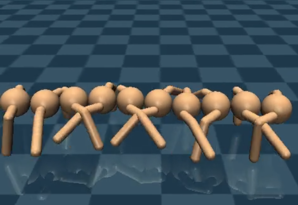
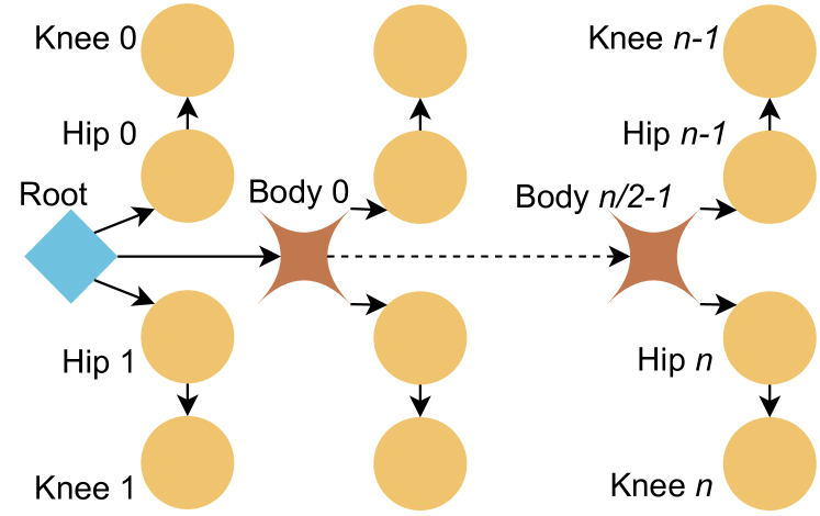
Figure 1: A MuJoCo rendering of Centipede-20 and its corresponding morphological graph.

2.4 NerveNet

NerveNet is an MPNN designed for locomotion control, based on the gated GNN architecture [32]. NerveNet uses the morphology (physical structure) of the agent as the basis for the GNN’s input graph $\mathcal{G}$, with edges representing body parts and nodes representing the joints that connect them.

NerveNet assumes an MDP where the state $s$ can be factored into input labels $\boldsymbol{V}$, which are fed to the GNN to generate output labels: $\mathbf{V}^{\prime}=\textsc{NerveNet}(\mathcal{G},\mathbf{V})$. These are then used to parameterise a normal distribution defining the stochastic policy: $\pi(a|s)={\mathcal{N}}(\mathbf{V}^{\prime},\text{diag}(\boldsymbol{\sigma}^{2}))$, where the standard deviation is a separate vector of parameters learned during training. Actions $a$ are vectors, where each element represents the force to be applied at a given joint for the subsequent timestep. The policy is trained using PPO, with parameter updates computed via the Adam optimisation algorithm [25].

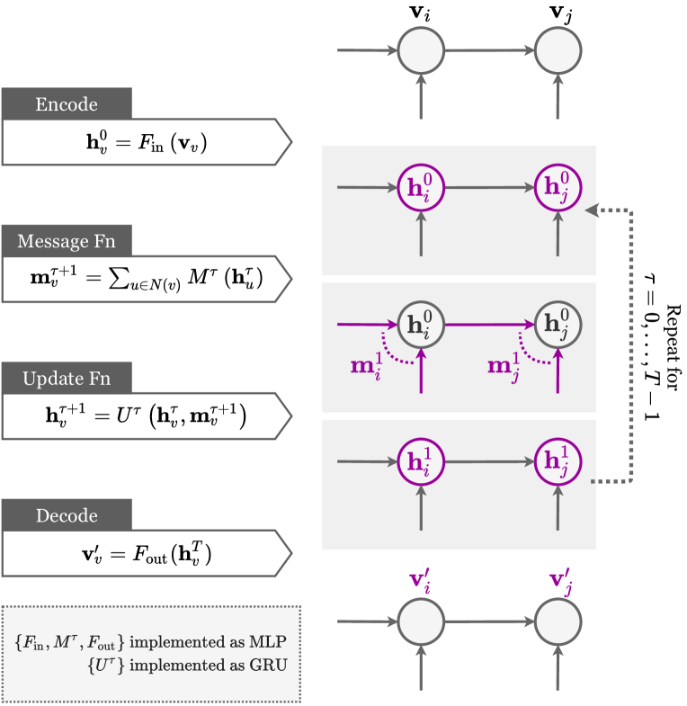
Figure 10: A visual representation of the NerveNet architecture. Updated representations at each step are indicated in purple. Given an input vector $\mathbf{v}$ at each node, NerveNet computes scalar outputs $\mathbf{v}^{\prime}$ through a series of propagation steps. Initially, the encoder is used to compute hidden states $\mathbf{h}$ at each node. These are passed into the message function, which computes an incoming message $\mathbf{m}$ for each node based on the hidden states of its neighbours. The update function then computes a new hidden state representation for each node based on the incoming message and the previous hidden state. The message function and update function then repeat their operations $T$ times, before feeding the final hidden states to the decoder, which produces outputs $\mathbf{v}^{\prime}$.

Internally, NerveNet uses an encoder $F_{\text{in}}$ to generate initial hidden states from input labels: $\mathbf{h}_{v}^{0}=F_{\text{in}}\left(\mathbf{v}_{v}\right)$. This is followed by a message function $M^{\tau}$ consisting of a single MLP for all layers $\tau$ that takes as input only the state of the sender node: $\mathbf{m}_{v}^{\tau+1}=\sum_{u\in N(v)}\text{MLP}\left(\mathbf{h}_{u}^{\tau}\right)$. The update function $U^{\tau}$ is a single gated recurrent unit (GRU) [9] that maintains an internal hidden state: $\mathbf{h}_{v}^{\tau+1}=\text{GRU}\left(\mathbf{m}_{v}^{\tau+1}\mid\mathbf{h}_{v}^{\tau}\right)$. NerveNet propagates through $\mathrm{T}$ layers of message-passing and node-updating, before applying a decoder $F_{\text{out}}$ to turn final hidden states into scalar node output labels: $\mathbf{v}^{\prime}_{v}=F_{\text{out}}(\mathbf{h}_{v}^{T})$. A diagram of the NerveNet architecture can be seen in Appendix A.4, Figure 10.

3 Analysing GNN Scaling Challenges

In this section, we use NerveNet to analyse the challenges that limit GNN s’ ability to scale. We focus on NerveNet as its architecture is more closely aligned with the GNN framework than alternative approaches to structured locomotion control (see Section 4). We use mostly the same experimental setup as Wang et al. [55], with details of any differences and our choice of hyperparameters outlined in Appendix A.2.

We focus on environments derived from the Gym [8] suite, using the MuJoCo [53] physics engine. The main set of tasks we use to assess scaling is the selection of Centipede-n agents [55], chosen because of their relatively complex structure and ability to be scaled up to high-dimensional input-action spaces.

The morphology of a Centipede-n agent consists of a line of n/2 body segments, each with a left and right leg attached (see Figure 1). The graph used as the basis for the GNN corresponds to the physical structure of the agent’s body. At each timestep in the environment, the MuJoCo engine sends a feature vector containing the positions of the agent’s body parts and the forces acting on them, expecting a vector to be returned specifying forces to be applied at each joint (full details of the state representation are given in Appendix A.2). The agent is rewarded for forward movement along the $y$-axis as well as a small ‘survival’ bonus for keeping its body within certain bounds, and given negative rewards proportional to the size of its actions and the magnitude of force it exerts on the ground.

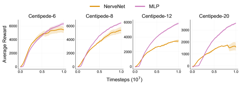
Figure 2: Comparison of the scaling of NerveNet relative to an MLP-based policy. Performance is similar for the smaller agent sizes, but NerveNet scales poorly to the larger agents.

Existing work applying GNNs to locomotion control tasks avoid training directly on larger agents, i.e., those with many nodes in the underlying graph representation. For example, Wang et al. [55] state that for NerveNet, “training a CentipedeEight from scratch is already very difficult”. Huang et al. [20] also limit training their SMP architecture to small agent types.

3.1 Scaling Performance

To demonstrate the poor scaling of NerveNet to larger agents, we compare its performance on a selection of Centipede-n tasks to that of an MLP policy. Figure 2 shows that for the smaller Centipede-n agents both policies are similarly effective, but as the size of the agent increases, the performance of NerveNet drops relative to the MLP. A visual inspection of the behaviour of these agents shows that for Centipede-20, NerveNet barely makes forward progress at all, whereas the MLP moves effectively.

As in previous literature [e.g., 55, 20], we are ultimately not concerned with outperforming MLP s on the specific training task, but rather matching their training task performance so that the additional benefits of GNN s can be realised. In our setting we particularly wish to leverage the strong transfer benefits of GNN s—as demonstrated by Wang et al. [55]—resulting from their capacity to process inputs of arbitrary size and structure.

In other words, the focus of this paper is on deriving a method that can close the gap in Figure 2, as doing so makes GNN s a better choice overall given the trained policy transfers better than the MLP equivalent (see Section 5 for experimental results).

Table 1: KL-divergence from the policy before each update to the policy after, calculated over each batch. We train on $10^{7}$ timesteps, recording in the table the mean taken over last $10\%$ of steps.

	Policy KL-divergence
Policy type	Centipede-6	Centipede-8	Centipede-12	Centipede-20
MLP	0.021	0.024	0.031	0.044
NerveNet	0.115	0.137	0.118	0.123

3.2 Unstable policy updates

As outlined in Section 2.2, one of the key challenges for on-policy RL is preventing individual updates from causing excessive changes in policy space (i.e., keeping it within the trust region). Table 1 shows the extent to which this problem contributes to NerveNet’s poor scaling, calculating the average KL-divergence from the pre-update policy to the post-update policy for both policy types. NerveNet has a consistently higher KL-divergence than the MLP policy, indicating that PPO finds it harder to ensure stable policy updates for the GNN.

We emphasise that this discrepancy persists even with carefully-tuned hyperparameter values for limiting policy divergence. Figure 3 shows the performance of NerveNet across a range of PPO $\epsilon$-clipping values (see Section 2.2), and in all cases NerveNet is still substantially inferior to an MLP (note that our experiments on NerveNet always use the best value of $\epsilon=0.1$ found here). As we demonstrate later (in Figure 8), controlling policy divergence effectively is a key component in making GNN s scale, but we see here that PPO alone does not control the divergence sufficiently to achieve this.

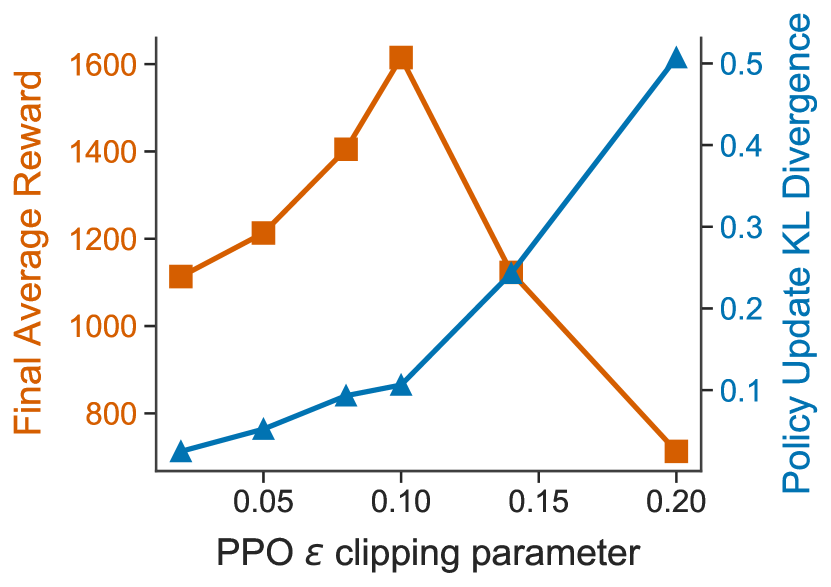
Figure 3: Final performance of NerveNet on Centipede-20 after ten million timesteps, across a range of $\epsilon$ clipping hyperparameter values. As $\epsilon$ increases (i.e., clipping is reduced) the KL divergence from the old to new policy (blue) increases. This improves performance (orange) up to a point, after which it begins to deteriorate.

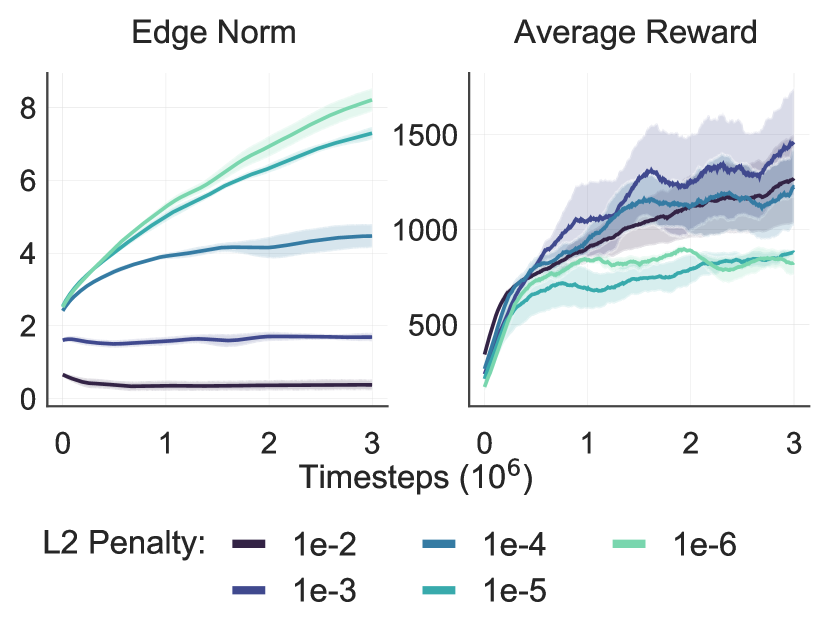
Figure 4: L2 regularisation for NerveNet’s message function across a range of values for the L2 penalty $\lambda$, trained on Centipede-20. Increasing this penalty reduces the L2 norm of the weights learned (left). Improved performance for higher values of $\lambda$ (right) indicates the presence of overfitting for the message function.

3.3 Overfitting in NerveNet

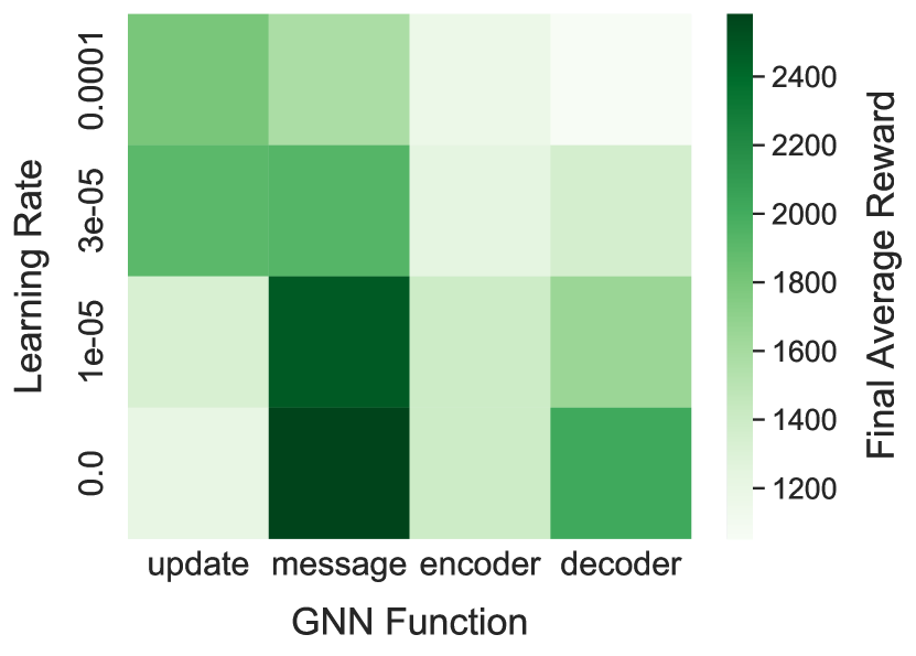
Figure 5: Colour-coded final NerveNet performance after 5M training steps on Centipede-20 when changing learning rates for individual GNN components, compared to the base learning rate of $3\times 10^{-4}$.

Excessive policy divergence resulting from updates can be understood as a form of overfitting. Whereas the supervised interpretation of overfitting implies poor generalisation from training to test set, in this case we are concerned with poor generalisation across state-action distributions induced by different iterations of the policy during training. Specifically, each update involves an optimisation step aiming to increase the expected reward over a batch of trajectories generated using the pre-update policy. The challenge for RL algorithms is that the agent is then evaluated and trained on trajectories generated using the post-update policy, i.e., a different distribution to the one optimised on.

For MPNN architectures like NerveNet, it is a known deficiency that in the supervised setting, message functions implemented as MLP s are prone to overfitting [16, p.55]. Here, we demonstrate that they also overfit (using the above interpretation) in our on-policy RL setting. Figure 4 shows the effect of applying L2 regularisation (a standard approach to reducing overfitting) to the NerveNet architecture. We regularise the parameters $\boldsymbol{\theta}$ of NerveNet’s message function MLP $M_{\boldsymbol{\theta}}$, adding a $\lambda||\boldsymbol{\theta}||_{2}^{2}$ term to our objective function. At the optimal value of $\lambda$ we see an improvement in performance (although still substantially inferior to using an MLP), indicating that the unregularised message-passing MLP s overfit.

We also investigate lowering the learning rate in different parts of the GNN, with the aim of identifying where overfitting is localised. If parts of the network are particularly prone to damaging overfitting, training them more slowly may reduce their contribution to policy instability across updates. Results for this experiment can be seen in Figure 5.

Not only does lowering the learning rate in parts of the model improve performance, but surprisingly the best performance is obtained when the encoder $F_{\text{in}}$, message function $M$ and decoder $F_{\text{out}}$ each have their learning rate set to zero. The encoder and decoder play a similar role to the message function, all of which are implemented as MLP s, whereas the update function $U$ is a GRU (we experimented with using an MLP update function, but found that this significantly reduced performance.).

3.4 Snowflake

Training with a learning rate of zero is equivalent to parameter freezing (e.g., Brock et al. [7]), where parameters are fixed to their initialised values throughout training. NerveNet can learn a policy with some of its functions frozen, as learning still takes place in the un-frozen functions. For instance, if we consider freezing the encoder, this results in an arbitrary mapping of input features to the initial hidden states. As we still train the update function that processes this representation, so long as key information from the input features is not lost via the arbitrary encoding, the update function can still learn useful representations. The same logic applies to using a frozen decoder or message function.

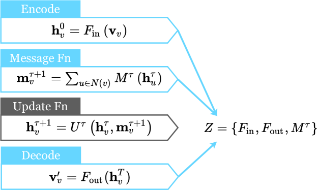
Figure 11: A visual representation of our Snowflake algorithm, as outlined in Section 3.4. Prior to training we select a fixed subset $\mathcal{Z}\subseteq\{F^{1}_{\boldsymbol{\theta}},\dots,F^{n}_{\boldsymbol{\theta}}\}$ of the GNN’s functions. For our experiments we use $\zeta=\{F_{\text{in}},F_{\text{out}},M^{\tau}\}$. Their parameters are then placed in Snowflake’s frozen set $\zeta=\{\boldsymbol{\theta}\mid F_{\boldsymbol{\theta}}\in Z\}$. During training, Snowflake excludes parameters in $\zeta$ from being updated by the optimiser.

Based on the effectiveness of parameter freezing within parts of the network, we propose a simple technique for improving the training of GNN s via gradient-based optimisation, which we name Snowflake (a naturally-occurring frozen graph structure). Snowflake assumes a GNN architecture made up internally of functions $F^{1}_{\boldsymbol{\theta}},\dots,F^{n}_{\boldsymbol{\theta}}$, where $\boldsymbol{\theta}$ denotes the parameters of a given function. Prior to training we select a fixed subset $\mathcal{Z}\subseteq\{F^{1}_{\boldsymbol{\theta}},\dots,F^{n}_{\boldsymbol{\theta}}\}$ of these functions. Their parameters are then placed in Snowflake’s frozen set $\zeta=\{\boldsymbol{\theta}\mid F_{\boldsymbol{\theta}}\in Z\}$. During training, Snowflake excludes parameters in $\zeta$ from being updated by the optimiser, instead fixing them to whatever values the GNN architecture uses as an initialisation. Gradients still flow through these operations during backpropagation, but their parameters are not updated. In practice, we found optimal performance for $\zeta=\{F_{\text{in}},F_{\text{out}},M^{\tau}\}$, i.e. when freezing the encoder, decoder and message function of the GNN. If not stated otherwise, this is the architecture we refer to as Snowflake in subsequent sections. A visual representation of Snowflake applied to the NerveNet model can be seen in Figure 11, Appendix A.4.

For our experiments, we initialise the values in the GNN using the orthogonal initialisation [44]. We found this to be slightly more effective for frozen and unfrozen training than uniform and Xavier initialisations [15]. For our message function, which has input and output dimensions of the same size, we find that performance with the frozen orthogonal initialisation is similar to that of simply using the identity function instead of an MLP. However, in the general case where the input and output dimensions of functions in the network differ (such as in the encoder and decoder, or in GNN architectures where layers use representations of different dimensionality), this simplification is not possible and freezing is required.

4 Related Work

Structured Locomotion Control

Several different graph neural network-like architectures [45, 5] have been proposed to learn policies for locomotion control. Wang et al. [55] introduce NerveNet, which trains a GNN based on the agent’s morphology, along with a selection of scalable benchmarks. NerveNet achieves multi-task and transfer learning across morphologies, even in the zero-shot setting (i.e., without further training), which standard MLP-based policies fail to achieve. Sanchez-Gonzalez et al. [42] use a GNN-based architecture for learning a model of the environment, which is then used for model-predictive control.

Huang et al. [20] propose Shared Modular Policies (SMP), which focuses on multi-task training and shows strong generalisation to out-of-distribution agent morphologies using a single policy. The architecture of SMP has similarities with a GNN, but requires a tree-based description of the agent’s morphology, and replaces size- and permutation-invariant aggregation with a fixed-cardinality MLP. Pathak et al. [39] propose dynamic graph networks (DGN), where a GNN is used to learn a policy enabling multiple small agents to cooperate by combining their physical structures.

Amorpheus [29] uses an architecture based on transformers [54] to represent locomotion policies. Transformers can be seen as GNN s using attention for edge-to-vertex aggregation and operating on a fully connected graph, meaning computational complexity scales quadratically with the graph size.

For all of these existing approaches to GNN-based locomotion control, training is restricted to small agents. In the case of NerveNet and DGN, emphasis is placed on the ability to perform zero-shot transfer to larger agents, but this still incurs a significant drop in performance.

Graph-Based Reinforcement Learning

GNNs have recently gained traction in RL due to their support for variable sized inputs and outputs, enabling new RL applications and enhancing the capabilities of agents on existing benchmarks.

Khalil et al. [24] apply DQN [38] to combinatorial optimisation problems using Structure2Vec [10] for function approximation. Lederman et al. [30] use policy gradient methods to learn heuristics of a quantified Boolean formulae solver, while Kurin et al. [28] use DQN [38] with graph networks [5] to learn the branching heuristic of a Boolean SAT solver. Klissarov and Precup [26] use a GNN to represent an MDP, which is then used to learn a form of reward shaping. Deac et al. [11] similarly use a GNN MPD representation to generalise Value Iteration Nets [51] to a broader class of MDPs.

Other approaches involve the construction of graphs based on factorisation of the environmental state into objects with associated attributes [4, 34]. In multi-agent RL, researchers have used a similar approach to model the relationship between agents, as well as between environmental objects [60, 21, 31]. In this setting, increasing the number of agents can result in additional challenges, such as combinatorial explosion of the action space. Our approach can be potentially useful to the above work, in improving scaling properties across a variety of domains.

Random Embeddings and Parameter Freezing

Embeddings represent feature vectors that have been projected into a new, typically lower-dimensional space that is easier for models to process. Bingham and Mannila [6] show that multiplying features by a randomly generated matrix (e.g., with entries sampled from a Gaussian distribution) preserves similarity well and empirically attains comparable performance to PCA. Wang et al. [57] use this approach to apply Bayesian Optimisation to high dimensional datasets by randomly projecting them into a smaller subspace. For natural language applications, commonly used pre-trained embeddings (e.g., word2vec [40], GloVe [37]) have been shown to offer only a small benefit over random embeddings on benchmark datasets [27, 12] and may offer no benefit on industry-scale data [3].

More generally, random embeddings can be induced by freezing typically-learned parameters within a model to fixed values throughout training. This approach has been explored for transformer architectures, where fixed attention weights (either Gaussian-distributed [59] or hand-crafted [41]) show no significant drop in performance, and even freezing intermediate feedforward layers still enables surprisingly effective learning [35]. A similar technique can also be found in common fine-tuning methods, where parameters are pre-trained on another, possibly unsupervised objective, but frozen during training except for the final layer [e.g., 58, 19].

5 Experiments

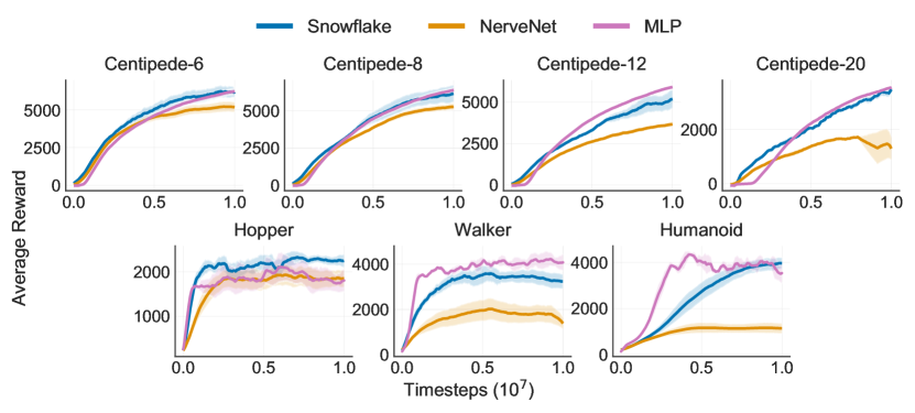
Figure 6: Comparison of the performance of Snowflake training, regular NerveNet and the MLP-based policy. Snowflake enables effective scaling to the larger agents, significantly outperforming regular NerveNet and comparable to using an MLP-based policy.

We present experiments evaluating the performance of Snowflake when applied to NerveNet, and compare against regular NerveNet and MLP policies. We evaluate each model on a selection of MuJoCo tasks, including three standard tasks from the Gym suite [8] and the Centipede-n agents from Wang et al. [55]. Note that we do not train on even larger Centipede-n agents due to wall-clock simulation time becoming prohibitively large.

All training statistics are calculated as the mean across six independent runs (unless specified otherwise), with the standard error across runs indicated by the shaded areas on each graph. The average reward typically has high variance, so to smooth our results we plot the mean taken over a sliding window of 30 data points. Further experimental details are outlined in Appendix A.2.

Scaling to High-Dimensional Tasks

Figure 6 compares the scaling properties of the regular NerveNet model with Snowflake. As the size of the agent increases, Snowflake significantly outperforms NerveNet with comparable asymptotic performance to the MLP. This indicates that Snowflake is successful in addressing the deficiencies of regular NerveNet training, and that freezing overfitting parameters is an effective training strategy in this setting. This holds true across locomotive agents with substantially different morphologies.

Zero-shot transfer

An important motivation for improving GNN scaling is to harness their transfer capabilities on large tasks. Regular NerveNet is limited by the fact that it can only effectively train on and transfer between small agent sizes. We show in Figure 7 that Snowflake attains exceptional zero-shot transfer performance across centipede sizes, surpassing alternative methods. Snowflake is the only method that can train a single policy that is effective on Centipede-20 through to 12.

Snowflake therefore achieves our initial objective: combining the strong training task performance of an MLP and the strong transfer performance of regular NerveNet. As a consequence, Snowflake-trained GNN s offer the most promising policy representation for locomotion control tasks where transfer is a desirable property.

Policy Stability and Sample Efficiency

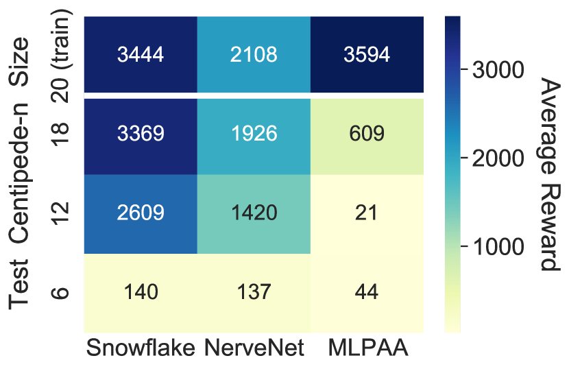
Figure 7: Zero-shot transfer performance for Snowflake, NerveNet, and MLP models trained on Centipede-20, evaluated across a range of sizes.

Figure 8: The effect of Snowflake on policy divergence and PPO clipping on Centipede-20. By freezing parts of the network that overfit, Snowflake reduces the policy KL divergence leading to less clipping during training.

By reducing overfitting in parts of the GNN, Snowflake mitigates the effect of harmful policy updates seen with regular NerveNet. As a consequence, the policy can train effectively on smaller batch sizes. This is demonstrated in Figure 9(a), which shows the performance of NerveNet trained regularly versus using Snowflake as the batch size decreases.

A potential benefit of training with smaller batch sizes is improved sample efficiency, as fewer timesteps are taken in the environment per update. However, smaller batch sizes also lead to increased policy divergence due to increased noise in the gradient estimate. When the policy divergence is too great, performance begins to decrease, limiting how small the batch can be. However due to a reduction in policy divergence as a result of Snowflake, we can afford to use smaller batch sizes while still keeping the policy under control. This provides a wider motivation for the use of Snowflake than just scaling to larger agents: it also improves sample efficiency across agents regardless of size.

The success of Snowflake in scaling to larger agents can also be understood in this context. Without Snowflake, for NerveNet to attain strong performance on large agents an infeasibly large batch size would be required, leading to poor sample efficiency. The more stable policy updates enabled by Snowflake make solving these large tasks tractable.

PPO Clipping

Snowflake’s improved policy stability also reduces the amount of clipping performed by PPO across each training batch. Figure 8 shows the percentage of state-action pairs that are clipped for regular NerveNet versus Snowflake on the Centipede-20 agent, as a result of reduced KL divergence.

When NerveNet is trained without using Snowflake a larger percentage of state-action pairs are clipped during PPO updates—a consequence of the greater policy divergence caused by overfitting. For PPO if too many data points reach the clipping limit during optimisation, the algorithm is only able to learn on a small fraction of the experience collected, reducing the effectiveness of training. One of Snowflake’s strengths is that because it reduces policy divergence it requires less severe restrictions to keep the policy within the trust region. The combination of this effect and the ability to train well on smaller batch sizes enables Snowflake’s strong performance on the largest agents.

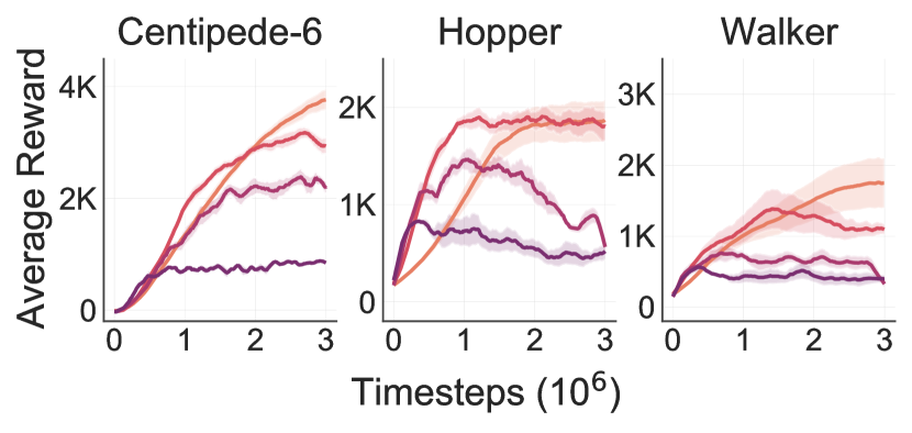
(a) NerveNet

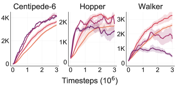
(b) Snowflake

Figure 9: Effectiveness of Snowflake across smaller batch sizes relative to standard NerveNet training. Snowflake is able to use smaller batch sizes, leading to improved sample efficiency. This is due to Snowflake reducing policy divergence across updates. Corresponding policy divergence plots can be found in the appendix.

 

6 Conclusion

We proposed Snowflake, a method that enables GNN-based policies to be trained effectively on much larger locomotive agents than was previously possible. We no longer observe a substantial difference in performance between using GNN s to represent a locomotion policy and the standard approach of using MLP s, even on the most challenging morphologies. As a consequence, GNN s now offer an alternative to MLP s for more than just simple tasks, and if the additional features of GNN s such as strong transfer are a requirement, then they are likely to be a more effective choice. We have also provided insight into why poor scaling occurs for certain GNN architectures, and why parameter freezing is effective in addressing the overfitting problem we identify.

Limitations of our work include the upper-limit on the size of agents we were able to simulate, the use of a single algorithm and architecture, and a focus only on locomotion control tasks. Future work may include applying alternative RL algorithms and GNN architectures, schemes for automating the selection of frozen parts of the network, and applying Snowflake-like methods to a wider range of learning problems.

Appendix A Appendix

A.1 Ethical Discussion

Our work addresses the problem of scaling GNNs for simulated locomotion control. As our data is generated and models trained solely in a simulated physics engine, the direct ethical implications of our work are minimal. However, we identify a number of potential risks emerging from extensions and alternative applications of our work. These centre on safety and bias concerns relating to robotic control, and transferring trained policies to new tasks/agents.

Robotic Control

As we only ever conduct rollouts of the policy in simulation, our agent is not trained with any safety constraints in mind, which would likely be a requirement for real-world applications. Safety is particularly relevant in the wider context of our work, as the aim of scaling GNNs to more complex and capable agents potentially gives rise to increasingly unsafe behaviours and outcomes in the worst-case. Future work is required to assess if existing RL safety methods [see 13] are as effective when GNN policies are used.

Although there are many beneficial use-cases for robotic agents, there is also potential for negative social outcomes. These may be through agents that are designed directly to do harm such as autonomous weapons, or that are used in socially irresponsible applications. We encourage researchers who use our methods in the pursuit of enabling new robotics applications to give consideration to such outcomes.

Policy Transfer

Although effective transfer has the benefit of reducing the need for further training on the target task, the resulting policy is inevitably biased towards the original training task. Algorithmic bias has been highlighted as a key challenge in recent years for AI fairness, particularly in the supervised setting [36], but also for RL algorithms [22].

In the case of GNN policy representations, this problem can arise if the graphs (and associated labels) trained on contain harmful bias. For instance, consider a GNN policy trained on (graph-based) traffic data to optimise an RL objective, such as cumulative journey time for route planning. If the training data consists only of roads in certain geographical areas, then transferring the policy to out-of-distribution areas may lead to unsuitable actions and a disparity in outcomes. Safety constraints satisfied on the training roads (e.g. limiting the number of road accidents) may also no longer be satisfied when transferring to new areas.

Ethical Conduct

Our training data consists entirely of simulated physical observations from the MuJoCo environment. There is no human-generated data used in our research, nor does any of our data relate to real-world phenomena (beyond the laws of physics and design of our agents). We are therefore satisfied that our use of data is appropriate and ethical.

A.2 Further Experimental Details

Here we outline further details of our experimental approach to supplement those given in Section 5.

Data Generation

As typical when training PPO on simulated environments, we train a policy by interleaving two processes: first, we perform repeated rollouts of the current policy in the environment to generate on-policy training data, and second, we optimise the policy with respect to the training data collected to generate a new policy, then repeat.

To improve wall-clock training time, for larger agents we perform rollouts in parallel over multiple CPU threads, scaling from a single thread for Centipede-6 to five threads for Centipede-20. Rollouts terminate once the sum of timesteps experienced across all threads reaches the training batch size. For our experiments the main computational cost as the agent size scales is the simulator, not the training of the network. Our GNN implementation is therefore not highly optimised as this is not our bottleneck.

For optimisation we shuffle the training data randomly and split the batch into eight minibatches. We perform ten optimisation epochs over these minibatches, in the manner defined by the PPO algorithm [48] (see Section 2.2).

Each experiment is performed six times and results are averaged across runs. The exceptions to this are Figure 5 where results are an average of three runs, and the Centipede-n tasks in Figure 6 where results are an average of ten runs.

Hyperparameter Search

Our starting point for selecting hyperparameters is the hyperparameter search performed by Wang et al. [55], whose codebase ours is derived from.

To ensure that we have the best set of hyperparameters for training on large agents, we ran our own hyperparameter search on Centipede-20 for Snowflake, as seen in Table 2.

Hyperparameter	Values
Batch size	512, 1024, 2048, 4096
Learning rate	1e-4, 3e-4, 1e-5
Learning rate scheduler	adaptive, constant
$\epsilon$ clipping	0.02, 0.05, 0.1, 0.2
GNN layers	2, 4, 10
GRU hidden state size	64, 128
Learned action std	shared, separate

Table 2: Hyperparameter search for Snowflake on Centipede-20. Values in bold resulted in the best performance.

Across the range of agents tested on, we conducted a secondary search over just the batch size, learning rate and $\epsilon$ clipping value for each model. For the latter two hyperparameters, we found that the values in Table 2 did not require adjusting.

For the batch size, we used the lowest value possible until training deteriorated. Using NerveNet, a batch size of 2048 was required throughout, whereas using Snowflake a batch size of 1024 was best for Walker, Centipede-20 and Centipede-12, 512 was best for Centipede-8 and Centipede-6, and 2048 for all other agents.

Wang et al. [55] provide experimental results for the NerveNet model, which we use as a baseline for our experiments. Out of the Centipede-n models, they provide direct training results for Centipede-8 (see the non-pre-trained agents in their Figure 5). Our performance results are comparable, but taken over many more timesteps. Their final MLP results appear slightly different to ours at the same point (they attain roughly 500 more reward), likely due to hyperparameter tuning for performance over a different time-frame.

They also provide performance metrics for trained Centipede-4 and Centipede-6 agents across the models compared (their Table 1). The results reported here are significantly less than the best performance we attain for both MLP and NerveNet on Centipede-6. We suspect this discrepancy is due to running for fewer timesteps in their case, but precise stopping criteria is not provided.

Computing Infrastructure

Our experiments were run on four different machines during the project, depending on availability. These machines use variants of the Intel Xeon E5 processor (models 2630, 2699 and 2680), containing between 44 and 88 CPU cores. As running the agent in the MuJoCo environment is CPU-intensive, we observed little decrease in training time when using a GPU; hence the experiments reported here are only run on CPUs.

Runtimes for our results vary significantly depending on the number of threads allocated and batch size used. Our standard runtime for Centipede-6 (single thread) for ten million timesteps is around 24 hours, scaling up to 48 hours for our standard Centipede-20 configuration (five threads). Our experiments on the default MuJoCo agents also take approximately 24 hours for a single thread.

State Space Description

The following is a breakdown of the information sent by the environment at each timestep to the different MuJoCo node types for the Centipede-n benchmark. Each different body and joint node receives its own version of this set of data:

Node Type	Observation Type	Axis
body	force	x
	force	y
	force	z
	torque	x
	torque	y
	torque	z
joint	position	x
	velocity	x
root	orientation	x
	orientation	y
	orientation	z
	orientation	a
	velocity	x
	velocity	y
	velocity	z
	angular velocity	x
	angular velocity	y
	angular velocity	z
	position	z
	force	x
	force	y
	force	z
	torque	x
	torque	y
	torque	z

Table 3: Description of the state space.

The root’s z-position (height) is relative to the (global) floor of the environment. For this benchmark the joints are hinge joints, meaning that there is only one degree of freedom, and its position value reflects the joint angle (note that x-axis here refers to the joint’s relative axis, not the global coordinate frame).

Our algorithm only strictly considers observations to come from joints rather than from body and root nodes. In this we follow the example set by NerveNet, which for the sake of simplicity concatenates body node observations with neighbouring joint observations, treating the resulting vector as a combined joint representation, which is then fed to the GNN.

A.3 Sources

Our source code can be found at https://github.com/thecharlieblake/snowflake/, alongside documentation for building the software and its dependencies. Our code is an extension of the NerveNet codebase: https://github.com/WilsonWangTHU/NerveNet. This repository contains the original code/schema defining the Centipede-n agents.

The other standard agents are taken from the Gym [8]: https://github.com/openai/gym. The specific hopper, walker and humanoid versions used are Hopper-v2, Walker2d-v2 and Humanoid-v2.

For our MLP results on the Gym agents, as state-of-the-art performance baselines have been well established in this case, we use the OpenAi Baselines codebase (https://github.com/openai/baselines) to generate results, to ensure the most rigorous and fair comparison possible.

The MuJoCo [53] simulator can be found at: http://www.mujoco.org/. Note that a paid license is required to use MuJoCo. The use of free alternatives was not viable in our case as our key benchmarks are all defined for MuJoCo.

A.4 Supplementary Figures

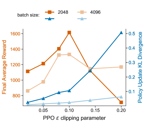
Figure 12: The effect of increasing the batch size on the influence of NerveNet’s $\epsilon$ clipping hyperparameter (see Figure 3) after ten million timesteps. Increasing the batch size reduces the underlying policy divergence. This makes the algorithm less sensitive to high values of $\epsilon$ (i.e. low clipping), but also leads to a drop in sample efficiency, reducing the maximum reward attained within this time-frame.

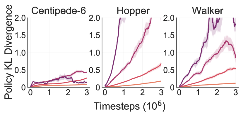
(a) NerveNet

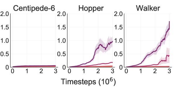
(b) Snowflake

Figure 13: Accompanying KL divergence plots for Figure 9(a). As Snowflake reduces the policy divergence between updates, smaller batch sizes can be used before the KL divergence becomes prohibitively large. This effect underlies the improved sample efficiency demonstrated.

 

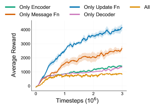
Figure 14: Ablation demonstrating the effect of only training single parts of the network (freezing the rest). The configuration of Snowflake we use for our experiments is equivalent to only training the update function, which is the most effective approach here, and all approaches are superior to training the entire GNN. For this experiment, we train on Centipede-6 using the small batch size of 256 in all cases. This setting was chosen as it demonstrates the difference in performance for these approaches most clearly.

References

- Abdolmaleki et al. [2018] Abbas Abdolmaleki, Jost Tobias Springenberg, Yuval Tassa, Rémi Munos, Nicolas Heess, and Martin A. Riedmiller. Maximum a posteriori policy optimisation. In ICLR, 2018.
- Amari [1997] SI Amari. Neural learning in structured parameter spaces-natural riemannian gradient. NIPS, pages 127–133, 1997.
- Arora et al. [2020] Simran Arora, Avner May, Jian Zhang, and Christopher Ré. Contextual embeddings: When are they worth it? In ACL, pages 2650–2663, 2020. doi: 10.18653/v1/2020.acl-main.236.
- Bapst et al. [2019] Victor Bapst, Alvaro Sanchez-Gonzalez, Carl Doersch, Kimberly Stachenfeld, Pushmeet Kohli, Peter Battaglia, and Jessica Hamrick. Structured agents for physical construction. In ICML, pages 464–474. PMLR, 2019.
- Battaglia et al. [2018] Peter Battaglia, Jessica B Hamrick, Victor Bapst, Alvaro Sanchez-Gonzalez, Vinicius Zambaldi, Mateusz Malinowski, Andrea Tacchetti, David Raposo, Adam Santoro, Ryan Faulkner, et al. Relational inductive biases, deep learning, and graph networks. CoRR, abs/1806.01261, 2018.
- Bingham and Mannila [2001] Ella Bingham and Heikki Mannila. Random projection in dimensionality reduction: applications to image and text data. In ACM, pages 245–250. ACM, 2001. doi: 10.1145/502512.502546.
- Brock et al. [2017] Andrew Brock, Theodore Lim, James M. Ritchie, and Nick Weston. Freezeout: Accelerate training by progressively freezing layers. CoRR, abs/1706.04983, 2017.
- Brockman et al. [2016] Greg Brockman, Vicki Cheung, Ludwig Pettersson, Jonas Schneider, John Schulman, Jie Tang, and Wojciech Zaremba. Openai gym. CoRR, abs/1606.01540, 2016.
- Cho et al. [2014] Kyunghyun Cho, Bart van Merrienboer, Çaglar Gülçehre, Dzmitry Bahdanau, Fethi Bougares, Holger Schwenk, and Yoshua Bengio. Learning phrase representations using RNN encoder-decoder for statistical machine translation. In EMNLP, pages 1724–1734. ACL, 2014. doi: 10.3115/v1/d14-1179.
- Dai et al. [2016] Hanjun Dai, Bo Dai, and Le Song. Discriminative embeddings of latent variable models for structured data. In ICML, volume 48 of JMLR Workshop and Conference Proceedings, pages 2702–2711. JMLR.org, 2016.
- Deac et al. [2020] Andreea Deac, Petar Veličković, Ognjen Milinković, Pierre-Luc Bacon, Jian Tang, and Mladen Nikolić. Xlvin: executed latent value iteration nets. In NeurIPS, NeurIPS Deep Reinforcement Learning Workshop, 2020.
- Dhingra et al. [2017] Bhuwan Dhingra, Hanxiao Liu, Ruslan Salakhutdinov, and William W. Cohen. A comparative study of word embeddings for reading comprehension. CoRR, abs/1703.00993, 2017.
- García and Fernández [2015] Javier García and Fernando Fernández. A comprehensive survey on safe reinforcement learning. J. Mach. Learn. Res., 16:1437–1480, 2015.
- Gilmer et al. [2017] Justin Gilmer, Samuel S. Schoenholz, Patrick F. Riley, Oriol Vinyals, and George E. Dahl. Neural message passing for quantum chemistry. In ICML, volume 70, pages 1263–1272. PMLR, 2017.
- Glorot and Bengio [2010] Xavier Glorot and Yoshua Bengio. Understanding the difficulty of training deep feedforward neural networks. In AISTATS, volume 9 of JMLR Proceedings, pages 249–256. JMLR.org, 2010.
- Hamilton [2020] William L. Hamilton. Graph representation learning. Synthesis Lectures on Artifical Intelligence and Machine Learning, 14(3):p55, 2020.
- Heess et al. [2017] Nicolas Heess, Dhruva TB, Srinivasan Sriram, Jay Lemmon, Josh Merel, Greg Wayne, Yuval Tassa, Tom Erez, Ziyu Wang, SM Eslami, et al. Emergence of locomotion behaviours in rich environments. CoRR, abs/1707.02286, 2017.
- Heintz et al. [2020] Aneesh Heintz, Vesal Razavimaleki, Javier Duarte, Gage DeZoort, Isobel Ojalvo, Savannah Thais, Markus Atkinson, Mark Neubauer, Lindsey Gray, Sergo Jindariani, et al. Accelerated charged particle tracking with graph neural networks on fpgas. CoRR, abs/2012.01563, 2020.
- Houlsby et al. [2019] Neil Houlsby, Andrei Giurgiu, Stanislaw Jastrzebski, Bruna Morrone, Quentin de Laroussilhe, Andrea Gesmundo, Mona Attariyan, and Sylvain Gelly. Parameter-efficient transfer learning for NLP. In ICML, volume 97 of Proceedings of Machine Learning Research, pages 2790–2799. PMLR, 2019.
- Huang et al. [2020] Wenlong Huang, Igor Mordatch, and Deepak Pathak. One policy to control them all: Shared modular policies for agent-agnostic control. In International Conference on Machine Learning, pages 4455–4464. PMLR, 2020.
- Iqbal et al. [2021] Shariq Iqbal, Christian A. Schröder de Witt, Bei Peng, Wendelin Boehmer, Shimon Whiteson, and Fei Sha. Randomized entity-wise factorization for multi-agent reinforcement learning. In ICML, pages 4596–4606, 2021.
- Jabbari et al. [2017] Shahin Jabbari, Matthew Joseph, Michael J. Kearns, Jamie Morgenstern, and Aaron Roth. Fairness in reinforcement learning. In ICML, volume 70, pages 1617–1626, 2017.
- Kakade [2001] Sham M. Kakade. A natural policy gradient. In NIPS, pages 1531–1538. MIT Press, 2001.
- Khalil et al. [2017] Elias B. Khalil, Hanjun Dai, Yuyu Zhang, Bistra Dilkina, and Le Song. Learning combinatorial optimization algorithms over graphs. In NIPS, pages 6348–6358, 2017.
- Kingma and Ba [2015] Diederik P. Kingma and Jimmy Ba. Adam: A method for stochastic optimization. In ICLR, 2015.
- Klissarov and Precup [2020] Martin Klissarov and Doina Precup. Reward propagation using graph convolutional networks. In NeurIPS, 2020.
- Kocmi and Bojar [2017] Tom Kocmi and Ondrej Bojar. An exploration of word embedding initialization in deep-learning tasks. In ICON, pages 56–64. NLP Association of India, 2017.
- Kurin et al. [2020] Vitaly Kurin, Saad Godil, Shimon Whiteson, and Bryan Catanzaro. Can q-learning with graph networks learn a generalizable branching heuristic for a SAT solver? In NeurIPS, 2020.
- Kurin et al. [2021] Vitaly Kurin, Maximilian Igl, Tim Rocktäschel, Wendelin Boehmer, and Shimon Whiteson. My body is a cage: the role of morphology in graph-based incompatible control. In ICLR, 2021.
- Lederman et al. [2020] Gil Lederman, Markus N. Rabe, Sanjit Seshia, and Edward A. Lee. Learning heuristics for quantified boolean formulas through reinforcement learning. In ICLR, 2020.
- Li et al. [2021] Sheng Li, Jayesh K. Gupta, Peter Morales, Ross E. Allen, and Mykel J. Kochenderfer. Deep implicit coordination graphs for multi-agent reinforcement learning. In AAMAS, pages 764–772. ACM, 2021.
- Li et al. [2016] Yujia Li, Daniel Tarlow, Marc Brockschmidt, and Richard S. Zemel. Gated graph sequence neural networks. In ICLR, 2016.
- Lim et al. [2019] Jaechang Lim, Seongok Ryu, Kyubyong Park, Yo Joong Choe, Jiyeon Ham, and Woo Youn Kim. Predicting drug-target interaction using a novel graph neural network with 3d structure-embedded graph representation. J. Chem. Inf. Model., 59(9):3981–3988, 2019. doi: 10.1021/acs.jcim.9b00387.
- Loynd et al. [2020] Ricky Loynd, Roland Fernandez, Asli Çelikyilmaz, Adith Swaminathan, and Matthew J. Hausknecht. Working memory graphs. In ICML, pages 6404–6414, 2020.
- Lu et al. [2021] Kevin Lu, Aditya Grover, Pieter Abbeel, and Igor Mordatch. Pretrained transformers as universal computation engines. CoRR, abs/2103.05247, 2021.
- Mehrabi et al. [2019] Ninareh Mehrabi, Fred Morstatter, Nripsuta Saxena, Kristina Lerman, and Aram Galstyan. A survey on bias and fairness in machine learning. CoRR, abs/1908.09635, 2019.
- Mikolov et al. [2013] Tomás Mikolov, Kai Chen, Greg Corrado, and Jeffrey Dean. Efficient estimation of word representations in vector space. In ICLR, 2013.
- Mnih et al. [2015] Volodymyr Mnih, Koray Kavukcuoglu, David Silver, Andrei A Rusu, Joel Veness, Marc G Bellemare, Alex Graves, Martin Riedmiller, Andreas K Fidjeland, Georg Ostrovski, et al. Human-level control through deep reinforcement learning. Nature, 518(7540):529–533, 2015. doi: 10.1038/nature14236.
- Pathak et al. [2019] Deepak Pathak, Christopher Lu, Trevor Darrell, Phillip Isola, and Alexei A. Efros. Learning to control self-assembling morphologies: A study of generalization via modularity. In NeurIPS, pages 2292–2302, 2019.
- Pennington et al. [2014] Jeffrey Pennington, Richard Socher, and Christopher D. Manning. Glove: Global vectors for word representation. In EMNLP, pages 1532–1543. ACL, 2014. doi: 10.3115/v1/d14-1162.
- Raganato et al. [2020] Alessandro Raganato, Yves Scherrer, and Jörg Tiedemann. Fixed encoder self-attention patterns in transformer-based machine translation. In EMNLP, pages 556–568. ACL, 2020. doi: 10.18653/v1/2020.findings-emnlp.49.
- Sanchez-Gonzalez et al. [2018] Alvaro Sanchez-Gonzalez, Nicolas Heess, Jost Tobias Springenberg, Josh Merel, Martin A. Riedmiller, Raia Hadsell, and Peter W. Battaglia. Graph networks as learnable physics engines for inference and control. In ICML, pages 4467–4476, 2018.
- Sarlin et al. [2020] Paul-Edouard Sarlin, Daniel DeTone, Tomasz Malisiewicz, and Andrew Rabinovich. Superglue: Learning feature matching with graph neural networks. In IEEE/CVF, pages 4937–4946, 2020. doi: 10.1109/CVPR42600.2020.00499.
- Saxe et al. [2014] Andrew M. Saxe, James L. McClelland, and Surya Ganguli. Exact solutions to the nonlinear dynamics of learning in deep linear neural networks. In ICLR, 2014.
- Scarselli et al. [2009] Franco Scarselli, Marco Gori, Ah Chung Tsoi, Markus Hagenbuchner, and Gabriele Monfardini. The graph neural network model. IEEE Trans. Neural Networks, 20(1):61–80, 2009. doi: 10.1109/TNN.2008.2005605.
- Schulman et al. [2015] John Schulman, Sergey Levine, Pieter Abbeel, Michael I. Jordan, and Philipp Moritz. Trust region policy optimization. In ICML, volume 37, pages 1889–1897. JMLR, 2015.
- Schulman et al. [2016] John Schulman, Philipp Moritz, Sergey Levine, Michael I. Jordan, and Pieter Abbeel. High-dimensional continuous control using generalized advantage estimation. In ICLR, 2016.
- Schulman et al. [2017] John Schulman, Filip Wolski, Prafulla Dhariwal, Alec Radford, and Oleg Klimov. Proximal policy optimization algorithms. CoRR, abs/1707.06347, 2017.
- Shen et al. [2018] Yantao Shen, Hongsheng Li, Shuai Yi, Dapeng Chen, and Xiaogang Wang. Person re-identification with deep similarity-guided graph neural network. In ECCV, volume 11219 of Lecture Notes in Computer Science, pages 508–526. Springer, 2018. doi: 10.1007/978-3-030-01267-0\_30.
- Stokes et al. [2020] Jonathan M Stokes, Kevin Yang, Kyle Swanson, Wengong Jin, Andres Cubillos-Ruiz, Nina M Donghia, Craig R MacNair, Shawn French, Lindsey A Carfrae, Zohar Bloom-Ackerman, et al. A deep learning approach to antibiotic discovery. Cell, 180(4):688–702, 2020.
- Tamar et al. [2016] Aviv Tamar, Sergey Levine, Pieter Abbeel, Yi Wu, and Garrett Thomas. Value iteration networks. In NIPS, pages 2146–2154, 2016.
- Thomas and Brunskill [2017] Philip S. Thomas and Emma Brunskill. Policy gradient methods for reinforcement learning with function approximation and action-dependent baselines. CoRR, abs/1706.06643, 2017.
- Todorov et al. [2012] Emanuel Todorov, Tom Erez, and Yuval Tassa. Mujoco: A physics engine for model-based control. In IEEE/RSJ International Conference on Intelligent Robots and Systems, pages 5026–5033. IEEE, 2012. doi: 10.1109/IROS.2012.6386109.
- Vaswani et al. [2017] Ashish Vaswani, Noam Shazeer, Niki Parmar, Jakob Uszkoreit, Llion Jones, Aidan N Gomez, Ł ukasz Kaiser, and Illia Polosukhin. Attention is all you need. In NIPS, volume 30, pages 5998–6008. Curran Associates, Inc., 2017.
- Wang et al. [2018] Tingwu Wang, Renjie Liao, Jimmy Ba, and Sanja Fidler. Nervenet: Learning structured policy with graph neural networks. In ICLR, 2018.
- Wang et al. [2020] Xuhong Wang, Ding Lyu, Mengjian Li, Yang Xia, Qi Yang, Xinwen Wang, Xinguang Wang, Ping Cui, Yupu Yang, Bowen Sun, and Zhenyu Guo. APAN: asynchronous propagate attention network for real-time temporal graph embedding. CoRR, abs/2011.11545, 2020.
- Wang et al. [2016] Ziyu Wang, Frank Hutter, Masrour Zoghi, David Matheson, and Nando de Freitas. Bayesian optimization in a billion dimensions via random embeddings. J. Artif. Intell. Res., 55:361–387, 2016. doi: 10.1613/jair.4806.
- Yosinski et al. [2014] Jason Yosinski, Jeff Clune, Yoshua Bengio, and Hod Lipson. How transferable are features in deep neural networks? In NIPS, pages 3320–3328, 2014.
- You et al. [2020] Weiqiu You, Simeng Sun, and Mohit Iyyer. Hard-coded gaussian attention for neural machine translation. In ACL, pages 7689–7700, 2020. doi: 10.18653/v1/2020.acl-main.687.
- Zambaldi et al. [2019] Vinícius Flores Zambaldi, David Raposo, Adam Santoro, Victor Bapst, Yujia Li, Igor Babuschkin, Karl Tuyls, David P. Reichert, Timothy P. Lillicrap, Edward Lockhart, Murray Shanahan, Victoria Langston, Razvan Pascanu, Matthew Botvinick, Oriol Vinyals, and Peter W. Battaglia. Deep reinforcement learning with relational inductive biases. In ICLR, 2019.