Periodic patterns displace active phase separation

Abstract

In this work we identify and investigate a novel bifurcation in conserved systems. This secondary bifurcation stops active phase separation in its nonlinear regime. It is then either replaced by an extended, system-filling, spatially periodic pattern or, in a complementary parameter region, by a novel hybrid state with spatially alternating homogeneous and periodic states. The transition from phase separation to extended spatially periodic patterns is hysteretic. We show that the resulting patterns are multistable, as they show stability beyond the bifurcation for different wavenumbers belonging to a wavenumber band. The transition from active phase separation to the hybrid states is continuous. Both transition scenarios are systems-spanning phenomena in particle conserving systems. They are predicted with a generic dissipative model introduced in this work. Candidates for specific systems, in which these generic secondary transitions are likely to occur, are, for example, generalized models for motility-induced phase separation in active Brownian particles, models for cell division or chemotactic systems with conserved particle dynamics.

1 Introduction

Patterns are ubiquitous in nature. They emerge spontaneously in a plethora of living or inanimate driven systems [1, 2, 3, 4, 5, 6, 7, 8, 9, 10], and their esthetic appeal is immediately apparent to all observers [1]. Prototypical patterns, such as stripes, hexagons and traveling waves can be found in various fluid-dynamical, chemical and biological systems and they often play a key role in various processes in nature. To name just a few examples: Convection patterns in fluid dynamical systems enhance the thermal transport [2, 6], protein dynamics in E. coli plays a key role in finding the cell center during the cell division process [11, 12, 13, 14], and the formation of patterns are the basis of successful survival strategies for vegetation in water-limited regions [8, 9].

The mechanisms that drive nonequilibrium patterns are as diverse as the systems in which they occur. Instabilities leading to patterns are usually divided into type I, II and III, which differ in their preferred wavenumber $q_{0}$ and/or in their frequency $\omega_{0}$ and the wavenumber dependence of the dispersion relation [2]. Despite their very different origins, nonequilibrium patterns of the type I and type III share common universal properties, which are covered by universal Ginzburg-Landau equations (GLEs) [15, 16, 17, 18, 19, 20, 21, 2, 22, 5, 4, 3]. They describe the dynamics of the envelope (resp. the order parameter field) of stationary and traveling stripe or oscillating patterns.

A number of nonequilibrium demixing phenomena with conserved particle dynamics attract increasing attention recently [23, 24, 25, 26, 27, 28, 29, 30, 31, 32]. Ultimately, these are type II instabilities, for which the theory is currently undergoing a lively development. Such nonequilibrium demixing phenomena include cell polarization [23, 24], chemotactically communicating cells [25, 26], motility induced phase separation (MIPS) in self-propelled Brownian particle systems [27, 28, 29, 30, 31] and also a very early model for the ion-channel density in a membrane [32].

Demixing phenomena in thermal equilibrium systems are long known and they are described by the Cahn-Hilliard (CH) mean-field model [33, 34, 35, 36]. It is very surprising that the CH equation describes also the generic order-parameter field for type II instabilities with particle conservation, i.e. also for non-equilibrium demixing phenomena [37, 38, 39, 40]. This was shown by generalizing the perturbation theory used to derive equations for unconserved order parameter fields [17, 18, 19, 20, 2, 22, 3] to cases with conserved order parameter fields [37]. Its application to the dynamical equations of chemotactic systems [37, 40], to models of cell polarization [37, 39] and to MIPS [38] results always directly in the generic CH equation. Accordingly, the coefficients of the CH equation now depend on the kinetic parameters of the respective system and it describes nonequilibrium rather than equilibrium transitions.

In the case of MIPS the CH model was extended to the active model B and the active model B+ by higher order nonlinear terms to describe interesting coarse-grained phenomena further away from the onset [41, 42, 43] with particular emphasis on the effects of noise. The perturbation theory in Ref. [37] extended to the next higher nonlinear order and applied to a mean-field theory for MIPS [29, 44] gives the generic structure of AMB+ [38] as well. Moreover, this perturbation-theoretic approach unambiguously links the parameters of AMB+ to the kinetic parameters of the mean field model in Refs. [29, 44]. In terms of this perturbation theory the deterministic part of AMB+ is a generic nonlinear extension of the CH model rather than an extension into nonequilibrium.

The perturbation theory from Ref. [37] systematically provides, in addition to the generic next higher nonlinear contributions, also a sixth-order spatial derivative of the order parameter field. This higher order derivative is not part of active model B+, but becomes indispensable beyond a finite distance from the threshold of MIPS and at larger amplitudes of the order parameter field. In this range, solutions without the sixth-order derivative then show unbounded growth. The conserved Swift-Hohenberg model+ (CoSH+) introduced in section 2 for a class of systems showing nonequilibrium phase separation includes this higher derivative and shows a novel secondary bifurcation in the nonlinear regime of active phase separation, which is characterized in section 3. There are two complementary scenarios of the secondary bifurcation, and they are described in section 4 and 5. In the section 6 we summarize our results, classify them and highlight further perspectives of this work.

2 Generic model for a conserved order parameter field

We introduce and investigate a nonlinear model for a real-valued conserved order parameter field $\psi(x,t)$, which is simultaneously an extension of the Cahn-Hilliard model [34, 35, 36] by the generic next higher order contributions and an extension of the conserved Swift-Hohenberg model [45] by the leading order nonlinear gradient terms,

$$\qquad\partial_{t}\psi=-\partial_{x}^{2}\Big{[}\varepsilon\psi+(D_{4}+\beta_{2}\psi)\partial_{x}^{2}\psi-D_{6}\partial_{x}^{4}\psi+\beta_{1}\psi^{2}-g\psi^{3}+\beta_{3}\left(\partial_{x}\psi\right)^{2}\Big{]}\,,$$ (1)

with $D_{4},D_{6},g>0$. Equation (1) is symmetric with respect to the transformation $(\psi,\beta_{1},\beta_{2},\beta_{3})\rightarrow-(\psi,\beta_{1},\beta_{2},\beta_{3})$. It can be written in the form of a conservation law $\partial_{t}\psi=-\partial_{x}j$ with $j=j(\psi,\partial_{x}\psi)$ and contains a number of models as special cases. For $D_{6}=\beta_{1}=\beta_{2}=\beta_{3}=0$ equation (1) reduces to the classic Cahn-Hilliard (CH) model in one spatial dimension [33, 34, 35, 36]. Using an $\varepsilon$-scaling the contributions including $D_{6},\beta_{2},\beta_{3}$ are shown to vanish in the limit of small control parameter values $\varepsilon$ in A.

For $D_{6}=0$ the model corresponds to the nonlinearly extended Cahn-Hilliard model for active phase separation [38], which was recently derived by a systematic perturbation calculation [37] from a dissipative mean-field model for MIPS in active colloids [44]. Equation (1) reduces for $D_{6}=\beta_{1}=0$ to the one-dimensional version of the so-called active model B+ with $K_{1}\not=0$ in reference [43]. In the case of vanishing coefficients $D_{6}=g=\beta_{1}=\beta_{2}=0$ the equation (1) reduces to the conserved Kuramoto-Sivashinsky model [46]. For the parameter set ${\beta_{i}=0}$ ($i=1,2,3$), ${D_{6}=1}$, ${D_{4}=-2}$ and ${\varepsilon=r-1}$ equation  (1) describes the conserved Swift-Hohenberg model for spatially periodic patterns [45], also known as the phase-field crystal model [47].

The 6th order derivative $D_{6}\partial_{x}^{6}\psi$ in the linear operator in equation (1) has been added in contrast to the models in Refs. [43, 38]. Without this higher order contribution model (1) will become structurally unstable for larger values of the control parameter. Above the onset of phase separation one has $\psi\propto\sqrt{\varepsilon}$ and $\psi$ takes positive and negative values equally likely. Therefore, the prefactor $D_{4}+\beta_{2}\psi$ may become small $D_{4}+\beta_{2}\psi\sim\sqrt{\varepsilon}$ for negative values of $\beta_{2}\psi<0$ or even negative for $D_{4}>0$. Moreover, in this parameter range close the threshold one has slow variations of the fields, i. e. $\partial_{x}^{2}\psi\sim O(\varepsilon)$, $\partial_{x}\sim O(\varepsilon^{1/4})$ and all contributions to equation (1) are of the same order $\propto\varepsilon^{2}$, including $\partial_{x}^{6}\psi$. This illustrates why equation (1) would be incomplete without the contribution $\partial_{x}^{6}\psi$. In this sense equation (1) is a consistent generic model being structurally stable also for small or negative values $D_{4}+\beta_{2}\psi\sim\sqrt{\varepsilon}$. Equation (1) is a systematic extension of the conserved Swift-Hohenberg model by leading order nonlinear gradient terms and therefore, we call it conserved Swift-Hohenberg model+ (CoSH+).

Equation (1) has the additional interesting property that its solutions obey a gradient dynamics

$$\partial_{t}\psi=\partial^{2}_{x}\left(\frac{\delta{\cal F}}{\delta\psi}\right)$$ (2)

for the parameter combination $\beta_{2}=2\beta_{3}$ with the functional

$${\cal F}(\psi)=\int dx\left[\frac{\psi^{4}}{4}-\frac{\beta_{1}\psi^{3}}{3}-\frac{\varepsilon}{2}\psi^{2}+\left(\frac{D_{4}}{2}+\beta_{3}\psi\right)\left(\partial_{x}\psi\right)^{2}+\frac{D_{6}}{2}\left(\partial_{x}^{2}\psi\right)^{2}\right].$$ (3)

In this work we focus either on the case without a gradient dynamics, especially on the parameter range $\beta_{2}\propto O(1)$ with $\beta_{3}=0$ or small values of $\beta_{3}$. In a second case we focus on the range with a gradient dynamics and its neighborhood $\beta_{2}\sim 2\beta_{3}$. In both ranges we find two different scenarios of a secondary transition taking place above the onset of phase separation.

Numerically we solve equation (1) with periodic boundary conditions on a spatial domain $(0,L)$ (see B for specifics). Unless stated otherwise, the following set of parameters is used throughout: $\beta_{2}=\sqrt{2}$, $D_{4}=0.15$, $D_{6}=1/6$ and $g=1$.

3 Phase separation and its transition to stable periodic patterns

In the range of small $\varepsilon$ the CoSH+ model (1) reduces to the classic CH-model as demonstrated in A by rescaling the CoSH+ model. This is also true for its solutions. It can be seen in figure 1a) for a small $\varepsilon=0.005$, where a stationary solution is shown that has the same form as typical monotonic domain-wall solutions of the CH-model connecting the plateau values $\psi_{0}=\pm\sqrt{\varepsilon\,}$ [34, 35].

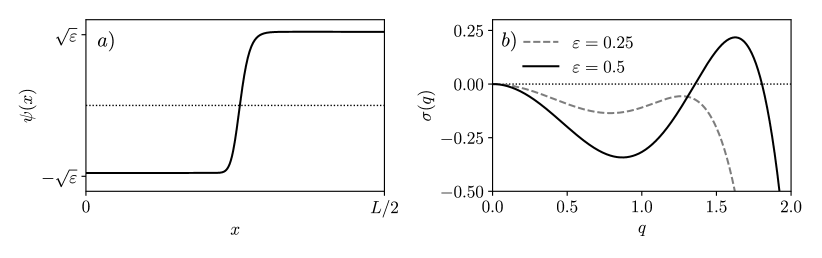
Figure 1: a) shows a one-domain solution of equation (1) for the parameters: $\varepsilon=0.005$, $D_{4}=0.15$, $D_{6}=1/6$, $\beta_{2}=\sqrt{2}$, $g=1$, $L=500$ and $\beta_{1}=\beta_{3}=0$. b) shows for two values of $\varepsilon$ the growth rate $\sigma(q)$, cf. equation (6), of perturbations with respect to the constant lower plateau value $\psi_{\ast}=-\sqrt{\varepsilon}$.

By increasing $\varepsilon$ as in 2a) up to $\varepsilon=0.06$, a domain wall solution as in figure 1 is deformed for finite $\beta_{2}>0$ ($\beta_{2}<0$) as damped oscillations develop at the lower (upper) plateau near the domain wall. In addition, the lower (upper) plateau widens and the amplitudes of both plateaus are shifted upwards (downwards).

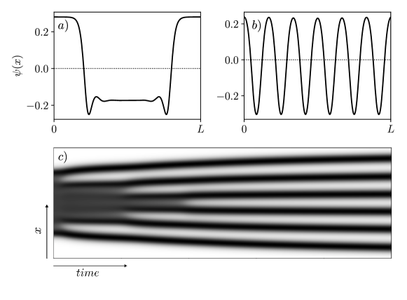
Figure 2: Part a) shows a stationary two-domain solution of equation (1) at $\varepsilon=0.06$ and in b) a stable spatially periodic pattern at $\varepsilon=0.065$ The transition between the two after a jump from $\varepsilon=0.06$ to $\varepsilon=0.065$ is shown in the space-time plot in part c). Further parameters are $D_{4}=0.15$, $D_{6}=1/6$, $\beta_{2}=\sqrt{2}$, $\beta_{1}=\beta_{3}=0$, $L=100$ and periodic boundary conditions were used.

To investigate whether these changes will eventually lead to an instability of domain wall solutions, as depicted in figure 2, we use the following ansatz

$$\psi(x,t)=\psi_{0}(x)+\psi_{1}(x,t)\,$$ (4)

and separate the primary state, $\psi_{0}(x)$, from contributions $\psi_{1}(x)$ of a possible secondary state to $\psi(x)$. This gives the nonlinear dynamical equation for $\psi_{1}$:

$$\partial_{t}\psi_{1}=-\partial_{x}^{2}\Big{[}\Big{(}\varepsilon+D_{4}\partial_{x}^{2}-D_{6}\partial_{x}^{4}-3\psi_{0}^{2}+2\beta_{1}\psi_{0}+\beta_{2}(\partial_{x}^{2}\psi_{0}+\psi_{0}\partial_{x}^{2})+2\beta_{3}(\partial_{x}\psi_{0})\partial_{x}\Big{)}\psi_{1}$$

$$-3\psi_{0}\psi_{1}^{2}-\psi_{1}^{3}+\beta_{1}\psi_{1}^{2}+\beta_{2}\psi_{1}\partial_{x}^{2}\psi_{1}\,+\beta_{3}(\partial_{x}\psi_{1})^{2}\Big{]}\,.$$ (5)

Further away from the domain walls and at small values of $\varepsilon$ the constant amplitude at the plateaus is approximately $\psi_{\ast}=\pm\sqrt{\varepsilon}$. In a first step we neglect the spatial variation of $\psi_{0}(x)$ near the domain walls, assume at the end of the plateaus periodic boundary conditions and the constant amplitude $\psi=\psi_{\ast}$ at the whole plateau. In this case equation (5) simplifies with $\beta_{1}=\beta_{3}=0$ to an equation with constant coefficients and its linear part can be solved by the ansatz $\psi_{1}=F\exp(\sigma t+iqx)$. The resulting growth rate has the following $q$-dependence

$$\sigma(q)=(\varepsilon-3\psi_{\ast}^{2})q^{2}-\left(D_{4}+\beta_{2}\psi_{\ast}\right)q^{4}-D_{6}q^{6}\,.$$ (6)

The prefactor in front of $\propto q^{4}$ may change its sign in the range $\psi_{\ast}\beta_{2}<-D_{4}$ even for $D_{4}>0$. In the range of a vanishing or even negative coefficient of $q^{4}$ the stabilizing higher-order derivative $D_{6}\partial_{x}^{6}\psi$ in equation (1) becomes crucial and ensures with $D_{6}>0$ the damping of short-scale perturbations in equation (6).

Beyond the onset of phase separation one has $\varepsilon>0$ and therefore a negative damping coefficient of $q^{2}$ in equation (6). In the case of a sign change of the prefactor of $q^{4}$ the growth rate $\sigma(q)$ develops besides $q=0$ a second extremum as indicated in figure 1b). The wavenumber at the finite-$q$ extremum is

$$q_{max}^{2}=\frac{1}{3D_{6}}\left[-\beta_{2}\psi_{\ast}-D_{4}+\sqrt{\left(\beta_{2}\psi_{\ast}+D_{4}\right)^{2}+3D_{6}(\varepsilon-3\psi_{\ast}^{2})}\right]\,,$$ (7)

if $\psi_{\ast}\beta_{2}>(3D_{6}\varepsilon-D_{4})$. For a sufficiently negative $D_{4}+\beta_{2}\psi_{\ast}$ the growth rate becomes positive in a finite $q$-range around its maximum $\sigma(q_{max})$, as indicated by the solid line in 1b). In the conserved Swift-Hohenberg model the $q$-dependence of the perturbation growth rate with respect to the homogeneous basic state shows a similar pattern forming behavior [45].

For the approximation $\psi_{\ast}=-\sqrt{\varepsilon}$ and $\beta_{2}>0$ the critical $\varepsilon$-value, above which $\sigma(q_{max})$ becomes positive, is given by

$$\varepsilon_{qc}=\frac{D_{4}^{2}}{\left(2\sqrt{2D_{6}}-\beta_{2}\right)^{2}}\,$$ (8)

with $\varepsilon=\varepsilon_{qc}$ at $q_{c}=q_{max}$. The formula shows that the threshold for an instability of the lower plateau value increases with $D_{4}^{2}$. If we account for the numerically observed upward shift in the lower plateau value, as in 2a), by an increase of approximately $25\%$ compared to $\psi_{\ast}\simeq-\sqrt{\varepsilon}$, then the threshold of the instability is reduced by about $50\%$ according to equation (6) compared to $\varepsilon_{qc}$.

The spatial variation of $\psi_{0}(x)$ near the domain wall causes spatially varying coefficients in the nonlinear equation (5). Such spatially varying coefficients can be represented by a Fourier series with locally varying Fourier amplitudes as demonstrated in reference [48]. It is known, that spatial modulations of parameters with a wavenumber twice that of the wavenumber of the pattern at onset lead to a reduction of the pattern threshold proportional to the amplitude of the modulation due to a so-called $1:2$ resonance [49, 50]. Here the spatially varying coefficients in equation (5) include Fourier modes with a wavenumber twice that of the wavenumber $q$ of $\psi_{1}$, but restricted to the range near the domain wall. These modulations are locally in $1:2$ resonance with $\psi_{1}$ in conjunction with the mentioned shift of $\psi_{\ast}$.

In figure 2 a) the two-domain solution at the control-parameter value $\varepsilon=0.06$ is stable. This $\varepsilon$-value is far below the threshold $\varepsilon_{qc}\simeq 0.334$ of an instability of a constant plateau solution $\psi_{\ast}=-\sqrt{\varepsilon}$ (for parameters as in figure 2). However, the shift of the plateau values $\psi_{\ast}$ and the local resonance lead to a shift of the onset of a secondary pattern such that a small $\varepsilon$-jump to $\varepsilon=0.065$ already destabilizes the two-domain solution in figure 2a) leading to the nonlinear evolution as shown in figure 2c).

According to the arguments above, the domain wall solution becomes unstable far below the predicted linear stability threshold $\varepsilon_{qc}\simeq 0.334$ for a constant plateau in the absence of spatial variations near the domain wall. As can be seen in figure 2c) the periodic pattern indeed nucleates near the domain walls and then evolves to a system filling extended periodic pattern as shown in figure 2b). It is quite surprising that the periodic solution spreads throughout the entire system instead of only over the lower plateaus. Note that for $\beta_{2}<0$ the upper plateau becomes unstable. The scenario of a periodic instability restricted to the lower plateau for $\beta_{2}>0$ (to the upper plateau for $\beta_{2}<0$) is described in section 5.

4 Multistability of spatially periodic patterns and transition scenarios

The extended spatially periodic patterns which displace active phase separation beyond the secondary instability as in figure 2c), are multistable in a finite wavenumber band, as we show in section 4.1. In addition, we demonstrate in section 4.2 that the transitions between stable periodic patterns of different wavenumbers exhibit the same universal behavior as those in classical pattern forming systems [51, 52, 53, 54, 55, 56, 57, 58, 59, 2]. Furthermore, the transition from phase separation to periodic patterns and back are shown to be hysteretic.

4.1 The Eckhaus stability band and transitions between periodic patterns

To address multistability of periodic patterns of different wavenumbers we first determine a stationary periodic, nonlinear solution $\psi_{s}$ by using an $N$-mode truncated Fourier ansatz

$$\psi_{s}(x)=\sum_{|\ell|\leq N}c_{\ell}e^{i\ell qx}\,,$$ (9)

with the conjugate symmetry $c_{\ell}=c^{*}_{-\ell}$ for the real field $\psi_{s}$ and $c_{0}=0$ as consequence of conservation. Using the ansatz (9) and projecting equation (1) onto the modes $\exp(inqx)$ for all $|n|\leq N$ yields coupled nonlinear equations for the Fourier amplitudes $c_{n}$. The $n$-th equation reads

$$\qquad 0=L(n,0)\,c_{n}-\sum_{|n-m-j|\leq N}c_{n-m-j}c_{m}c_{j}+\sum_{|n-m|\leq N}g(n,m)\,c_{n-m}c_{m}\,,$$ (10)

where for convenience we have introduced:

$$L(n,k) =\varepsilon-D_{4}\,(k+nq)^{2}-D_{6}\,(k+nq)^{4}\,,$$

$$g(n,m) =\beta_{1}-\beta_{2}\,(mq)^{2}-\beta_{3}\,(n-m)mq^{2}\,.$$ (11)

Equations (10) are solved numerically for a given set of system parameters and fixed values of $\varepsilon$ and $q$. In equation (9) modes with even and uneven values of $\ell$ are coupled in accordance with the broken $\pm$ symmetry of the equation as seen in figure 2b). The solutions of interest are dominated mostly by the amplitude $c_{1}$. While still significant, higher modes decay quickly allowing us to use $N=10$ for the calculation of $\psi_{s}$.

Similar as for $\psi_{0}(x)$ above we also investigate the linear stability of the stationary solution $\psi_{s}(x)$ with respect to a small perturbation $\psi_{p}(x,t)$. In this case one replaces in equation (5) $\psi_{0}$ by $\psi_{s}$. With $\psi_{s}$ given by equation (9) the part of equation being linear in $\psi_{1}$ (5) can be solved with a Floquet ansatz for $\psi_{1}=\psi_{p}$,

$$\psi_{p}(x,t)=e^{\sigma t}e^{ikx}\sum_{|m|\leq N}a_{m}e^{imqx}\,$$ (12)

and real Floquet exponent $k$. Using this ansatz for the linear part of equation (5) and projecting this equation onto $\exp[i(k+nq)x]$, we obtain the following linear eigenvalue problem for the coefficients $a_{n}$:

$$\sigma a_{n}= (k+nq)^{2}\,L(n,k)\,a_{n}-3(k+nq)^{2}\sum_{|n-m-j|\leq N}c_{n-m-j}c_{m}a_{j}$$ (13)

$$\hskip 71.13188pt+\sum_{|n-m|\leq N}h(n,m,k)\,c_{n-m}a_{m}\,,$$

where we have introduced in addition:

$$h(n,m,k)=2\beta_{1} -\beta_{2}(k+nq)^{2}[(k+mq)^{2}+(n-m)^{2}q^{2}]$$ (14)

$$-2\beta_{3}(k+nq)^{2}(k+mq)(n-m)q\,.$$

By determining the eigenvalues via equation (13), we identify the parameter ranges wherein one finds stable periodic solutions $\psi_{s}(x)$, i. e. wherein the eigenvalue with the largest real part $\sigma_{m}(k)$ is still negative:

$$\max_{k}\,\textrm{Re}\,\big{\{}\sigma_{m}(k)\big{\}}<0.$$ (15)

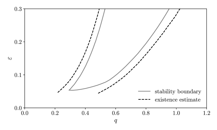
Figure 3: The solid line marks the boundary of the Eckhaus stability band of stable periodic solutions of the generic model (1) in the $\varepsilon-q$ plane for a given parameter set as given in figure 1. Unstable periodic solutions are numerically found in a wider range outside the Eckhaus band, at least in the ranges between the solid and dashed lines.

The so-called Eckhaus stability boundary is determined by $\max_{k}\,\textrm{Re}\,\big{\{}\sigma_{m}(k)\big{\}}=0$. It is displayed as the solid line in figure 3 for the parameter set given in figure 1. Between the Eckhaus stability boundary and the dashed lines we still find numerically stationary periodic solutions, but they are unstable.

Spatially periodic patterns $\psi_{s}$ with wavenumbers chosen from within the Eckhaus band, i.e. the area enclosed by the solid line in figure 3, are all linearly stable. This type of multistability is known to occur in a number of other pattern forming systems beyond a primary instability [60, 51, 52, 53, 54, 55, 56, 57, 58, 59, 2]. The insight that stationary, spatially periodic solutions predicted to occur beyond a secondary instability in systems with conserved order parameter fields share this generic property of multistability with a great number of other systems [60, 51, 52, 53, 54, 55, 56, 57, 58, 59, 2] is central to this work.

In contrast to other systems with spatially periodic patterns the shape of the stable Eckhaus band at its bottom in figure 3 is not parabolic. Most of the commonly known spatially periodic patterns emerge above a primary instability out of a homogeneous basic state that is symmetric with respect to spatial reflections and translations. In these cases the Eckhaus stability band has a parabolic shape near its minimum. Here in this work the secondary bifurcation to a spatially periodic patterns takes place after a primary bifurcation to phase separation and in the state of phase separation both symmetries are absent.

4.2 Transition scenario to and between extended periodic patterns

The similarities to other nonequilibrium stripe pattern are highlighted further in the way the solutions of the CoSH+ model in equation (1) respond to changes in the control parameter or the wavenumber beyond the secondary instability. This is demonstrated in figure 4 for a generic property of periodic patterns.

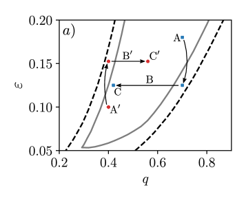
Figure 4: Two typical transition scenarios between stable periodic patterns are shown. At first one starts at $A$ in the $q-\varepsilon$ plane with a stable solution $A$ shown in part b). We then make a downward $\varepsilon$-jump from $A$ in the stable range in the $\varepsilon-q$ plane to the unstable range at $B$. The solution evolves then via an intermediate transient solution as shown by $B$ in part b) to a stable periodic solution C shown in part b) at the parameters marked by $C$ in part a). In the second scenario we start with a stable solution $A^{\prime}$ shown in part c) at the parameters $(q,\varepsilon)$ marked by$A^{\prime}$ in a). After an upward $\varepsilon$ jump from the stable $A^{\prime}$ to the unstable point $B^{\prime}$ in part a) the stable solution $A^{\prime}$ in c) evolves via transients as $B^{\prime}$ in part c) to a stable solution $C^{\prime}$ in c) at the parameters $C^{\prime}$ in a).

Figure 4a) depicts two examples of transition scenarios: In the first one, $A\to C$, a linearly stable periodic solution inside the Eckhaus band is quenched to the unstable range between the band and existence estimate. The system reacts to this change by reducing the wavenumber of the pattern via a series of transient states $B$ to arrive at $C$ back inside the Eckhaus band. Figure 4b) shows the corresponding initial stable state $A$, an example of a transient $B$ and the final state $C$. In the second scenario $A^{\prime}\to C^{\prime}$, we jump upwards into the unstable range and the system reacts by increasing the pattern wavenumber via transients $B^{\prime}$ to arrive at $C^{\prime}$ within the band. Figure 4 c) again shows the corresponding initial stable, the final stable periodic solution and an example of a transient $B^{\prime}$. Note that in both scenarios the shift in $\varepsilon$ is accompanied by a shift in the amplitude, which increases and decreases with the control parameter.

These transition scenarios of periodic states after parameter changes as shown in figure 4 are also observed for spatially periodic patterns in models with unconserved order parameters [52], in electrohydrodynamic convection in nematic liquid crystals [51] and in experiments with periodic patterns in Taylor-vortex flows [54]. Note that in these examples the transition scenarios have been observed for patterns that emerge out of a homogeneous basic state. In contrast, periodic patterns in our example emerge from a phase-separated state with broken translational and the reflection symmetry. Nevertheless, the transition scenarios for periodic patterns in a conserved model as shown in figure 4 are generic as in all the previous examples.

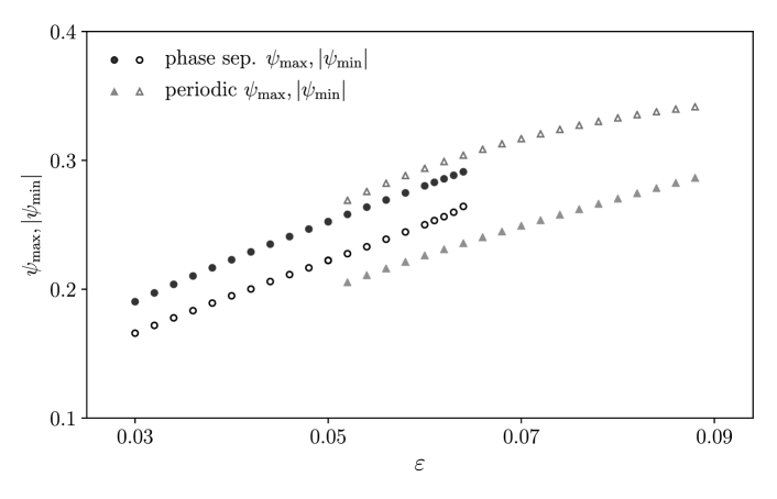
Figure 5: The maximum value $\psi_{max}$ and the magnitude of the minimal value $|\psi_{min}|$ of steady state solutions in simulations of equation (1) are given as a function of $\varepsilon$: Circles correspond to the amplitude $\psi_{max}$ (filled circles) and $|\psi_{min}|$ (open circles) during phase separation and the triangles mark the amplitudes of periodic solutions. If one starts with a state of phase separation the transition to spatially periodic solutions takes place by increasing $\varepsilon$ at around $\varepsilon\approx 0.065$ for the parameters given in figure 1. Starting with periodic solution, this will be stable below $\varepsilon\approx 0.065$, i. e. the secondary transition between phase separation and periodic patterns is hysteretic.

Due to the quadratic nonlinearities including $\beta_{2}$ and $\beta_{3}$ in equation (1), the maximal amplitudes $\psi_{max}$ and $|\psi_{min}|$ differ in both the phase separated state and the periodic state, cf. figure 2a),b). Plotting them as functions of increasing $\varepsilon$ one finds at the transition from phase separation (circles) to the periodic state (triangles) a jump in both amplitudes as shown in figure 5. Repeating the same by starting with a periodic pattern and decreasing $\varepsilon$ one finds the hysteresis of the transition as shown in figure 5.

By increasing $\varepsilon$, the transition scenario from phase separation to periodic states is similar as shown in figure 2c). The wavenumber of the final state is always within the Eckhaus-stable band in figure 3, whereby the wavenumber of the final periodic state may depend on the spatial structure of phase separation, i. e. on the distribution of the domain walls just before the transition takes place.

Starting with a periodic pattern, a sufficient reduction of $\varepsilon$ leads latest at the lower boundary of the Eckhaus stability band to a transition to phase separation. Since the spatial structure of the state of phase separation is multifaceted in long systems, the transition dynamics from periodic pattern to phase separation is in general less universal and rather complex.

The hysteretic transition scenario shown in figure 5 for $\beta_{1}=\beta_{3}=0$ will not change very much for finite but not to large parameter values $\beta_{3}$ and $\beta_{1}$. However, in the range $\beta_{2}\sim 2\beta_{3}$ we find a different transition scenario as described in the next section 5.

5 Stable secondary hybrid states

For the parameter combination $\beta_{2}=2\beta_{3}$ model (1) has the surprising property of a gradient dynamics as described by equations (2) and (3). The stability analysis of a constant plateau solution in section 3 is independent of $\beta_{3}$ and so the threshold $\varepsilon_{qc}$ remains unaltered. The dynamics and stationary solutions above $\varepsilon_{qc}$, however, differ greatly from those described in sections 3 and 4 for $\beta_{3}=0$. Note that for $\beta_{2}<0$ the upper instead of of the lower plateau becomes unstable, but the scenario is otherwise unchanged.

We find in a range around $\beta_{2}\sim 2\beta_{3}$ a further novel transition from the state of phase separation, with many plateau areas of different length, to a hybrid state, where constant plateaus alternate with spatially periodic patterns, as shown for example in a shorter system with only two domain walls in figure 6. Similar areas are occupied by the plateaus and the periodic states according to the conservation of the field $\psi(x,t)$, but by increasing the distance $\varepsilon-\varepsilon_{qc}$, the region occupied by a periodic state increases slightly as indicated in figure 6 from part b) to c).

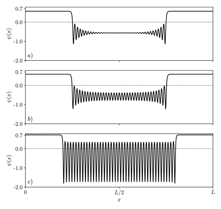
Figure 6: Stationary solutions of equation (1) are shown for three different values of the control parameter $\varepsilon=0.32$ in a), $\varepsilon=0.34$ in b) and $\varepsilon=0.5$ in c) for the parameter combination $\beta_{2}=2\beta_{3}=\sqrt{2}$ and $\beta_{1}=0$, where the solutions of equation (1) follow according to equations (2) and (3) a gradient dynamics. The length is $L=320$ and further parameters as in figure 2.

In the range $\beta_{2}\simeq 2\beta_{3}$ the secondary periodic pattern occurs again at first locally near the domain walls via wavy overshoots caused by the higher order spatial derivative. Therefore, localized finite amplitude patterns occur already below the threshold $\varepsilon_{qc}$, as indicated in figure 6a) at $\varepsilon=0.32<\varepsilon_{qc}=0.334$ (for the parameters used), but do not invade the lower plateau range. Patterns localized near the domain walls in the range $\varepsilon\lesssim\varepsilon_{qc}$, as in figure 6a), decay exponentially with the distance from the domain walls and the decay length increases with decreasing values of $D_{6}$.

A numerical solution of equation (1) shows that the amplitude of the periodic pattern in the middle between the two domain walls increases or decreases continuously $\propto\sqrt{\varepsilon-\varepsilon_{qc}}$ by increasing or decreasing $\varepsilon$. Therefore, the transition from the state of phase separation to the hybrid state is continuous and not hysteretic in spite of its local onset near the domain walls.

We have confirmed this numerical observation by a two-mode approximation $\psi_{hyb}=\psi_{\ast}+A\cos(q_{max}x)$. By choosing this ansatz we assume a long lower plateau at $\psi_{\ast}$ and periodic boundary conditions at its ends, i. e. we neglect the effects of the domain walls at the ends of a long plateau. In this case we obtain in agreement with our numerical observation that the amplitude $A$ is real with $A^{2}>0$ only in the range of $\varepsilon>\varepsilon_{qc}$. One finds $\psi_{hyb}$ with $A\not=0$ only in the range $\varepsilon>\varepsilon_{qc}$. The constant plateaus with $A=0$ corresponds to a local maximum, i. e. the functional has for finite $A$ a lower value than for $A=0$.

6 Summary and discussions

We discovered two new secondary bifurcation scenarios in systems described by conserved order parameter fields. Both scenarios occur by increasing the control parameter further after the primary bifurcation into active phase separation. In the first case, phase separation is stopped and completely replaced by an extended, system-filling, spatially periodic pattern. It is stable for different values of the wavenumber that belong to the so-called Eckhaus stability band, which we have determined for our model as shown in figure 3. The multistability of patterns with different wavenumbers is universal [51, 52, 53, 54, 55, 56, 57, 58, 59, 2]. It has been found experimentally and theoretically in a considerable number of nonequilibrium pattern forming systems with unconserved order parameter fields [51, 52, 53, 54, 55, 56, 57, 58, 59, 2]. As we have shown here, this multistability also applies for periodic patterns beyond a secondary bifurcation in systems with a conserved order parameter field.

The second bifurcation scenario describes a transition from active phase separation to a novel and stable nonlinear hybrid state. These hybrid solutions are spatial alternations between sections of spatially constant and spatially periodic states. Surprisingly, this spatially alternating coexistence of different spatial structures is stable. The subranges occupied by the homogeneous and periodic states may vary in space, but due to the conservation law both occupy similar areas immediately above the transition to the hybrid state. With increasing distance of the control parameter from the secondary threshold, the regions occupied by the periodic states increases slightly.

The basis of our novel results is the CoSH+ model in equation (1), which we introduced with this work. This model is a further step within a recent systematic and dynamic development for nonequilibrium systems described by conserved order parameter fields that we mention shortly. It has been found recently, that the weakly nonlinear behavior of several demixing phenomena in systems far from equilibrium are also described at leading order by the classic Cahn-Hilliard equation [37, 38, 39, 40] . This was demonstrated exemplarily for collective demixing phenomena in chemotactic systems [37, 40], for models of cell polarization [37, 39] and motility induced phase separation (MIPS) in active Brownian particle systems [38]. Previously, for modeling MIPS further away from its onset an extension of the CH model to the next higher nonlinear order, i. e. $\partial_{x}^{2}(\psi\partial_{x}^{2}\psi)$ and $\partial_{x}^{2}(\partial_{x}\psi)^{2}$, was suggested with the introduction of active model B+ [41, 43]. One of the two nonlinear extensions contributes to the prefactor $D_{4}+\beta_{2}\psi$ of $\partial_{x}^{4}\psi$ in the active model B+ and in the CoSH+ model (1). This prefactor may change its sign at larger amplitudes of the order parameter field. In this range the contribution $D_{6}\partial_{x}^{6}\psi$ is according to our perturbation theory of the same order as the nonlinear extensions. It is indispensable in this range to avoid dangerous large wavenumber instabilities after sign change of $D_{4}+\beta_{2}\psi$. Our model in (1) includes the sixth order derivative, similar as the conserved Swift-Hohenberg (CSH) model in reference [45], and it is in this sense an extension of the conserved SH model by generic leading order nonlinear gradient terms. Accordingly, we call it in section 2 the conserved Swift-Hohenberg model+ (CoSH+ model).

The spatially varying sign change of the prefactor $D_{4}+\beta_{2}\psi$ in equation (1) is the origin of the two novel bifurcation scenarios. This sign change is qualitatively similar to the Lifshitz point in pattern formation, found near the so-called oblique-roll instability in electroconvection in nematic liquid crystals, where the coefficient of a higher order spatial derivative undergoes a similar change in sign, but spatially homogeneously [61, 62, 63, 64].

Secondary bifurcations of, for example, stripe patterns are known in the field of classical pattern formation with unconserved order parameter fields [65, 66, 67, 68, 69, 70, 71, 2]. However, to the best of our knowledge there is so far no further example of a secondary bifurcation that evolves in a conserved nonequilibrium system out of active phase separation into stable nonlinear periodic pattern.

The existence of stability bands of periodic patterns, which we found for our first secondary bifurcation scenario, is a universal and robust phenomenon in nonlinear physics. To add or to remove a periodic unit (wavelength) of a pattern requires strong local deformations of the pattern, which cannot be driven by small inherent fluctuations. Therefore, in the absence of strong external deformations, periodic patterns remain stable at a wavenumber within the Eckhaus band. It is an important result of our work that this robust behavior of periodic patterns applies also to patterns beyond the secondary bifurcation in conserved systems. This robust stability of periodic patterns in conserved systems is also highly relevant for modeling cell division, where it possibly helps to find the center of a cell with great certainty, before it divides into two equally sized daughter cells carrying the same genetic information [72, 73].

In some former studies active phase separation was changed into a bifurcation to spatially periodic patterns by the introduction of additional kinetic effects that violate conservation laws and therefore change the bifurcation type [74, 75, 76]. For such a kinetically changed primary bifurcation from phase separation to periodic patterns, the notion arresting phase separation was coined [76]. Note that this is a crucial difference between these examples and our work. The transition to periodic patterns occurs in our work via a secondary bifurcation under the retention of the conservation conditions.

An extension of the model in equation (1) to two spatial dimensions is a further promising perspective. It is very likely that our results obtained for one spatial dimension lead in two dimensions to further interesting secondary bifurcation scenarios, for example, due to the broken up-down symmetry one expects at even lower values of the control parameter a secondary bifurcation to hexagonal patterns.

For pattern forming systems with unconserved order parameters a number of interesting finite size, inhomogeneity, noise and boundary effects on periodic patterns are known [77, 68, 49, 50, 78, 79, 48, 72, 80]. In contrast, such effects on periodic patterns in conserved systems, including those beyond secondary bifurcations, are unexplored so far.

Candidates of specific systems where the described phenomena are expected as well, are, for example, generalized chemotactic systems (see e. g. [40]), Brownian particle systems showing motility induced phase separation in the presence of quorum sensing [81] and cell biology, where periodic patterns play a key role in finding the cell center so that cells divide into equal parts with the same amount of genetic information [73].

Appendix A Significance of higher order corrections

In this appendix, we show as in reference [38] that contributions to our model (1), which go beyond the classic Cahn-Hilliard model, vanish in the limit of small values of the distance $\varepsilon$ from the onset of phase separation. For this we rescale time, space and amplitude in equation (1) such that the part of the classic CH in equation (1) becomes dimensionless: $t^{\prime}=\varepsilon^{2}t$, $x^{\prime}=\sqrt{\varepsilon}x$ and $\psi^{\prime}=\psi/\sqrt{\varepsilon}$. In addition we choose $\beta_{1}=\varepsilon\beta_{1}^{\prime}$, because the quadratic term at leading order can be removed by adding a constant. This allows us to rewrite equation (1) with a dimensionless classic CH part in the following form:

$$\partial_{t^{\prime}}\psi^{\prime} = -\partial_{x^{\prime}}^{2}\left[\psi^{\prime}+\partial_{x^{\prime}}^{2}\psi^{\prime}-\psi^{\prime 3}\right]$$ (16)

$$+\sqrt{\varepsilon}\partial_{x^{\prime}}^{2}\left[\beta_{2}\psi^{\prime}\partial_{x^{\prime}}^{2}\psi^{\prime}+\beta_{3}\left(\partial_{x^{\prime}}\psi^{\prime}\right)^{2}+\beta_{1}^{\prime}\psi^{\prime 2}\right]+\varepsilon\partial_{x^{\prime}}^{6}\psi^{\prime}\,.$$

Therefore, all contributions which do not belong to the leading order classic Cahn-Hilliard model vanish in the limit of small $\varepsilon$. This behavior explains, why in figure 1a) the solution of model (1) has in the limit of small $\varepsilon$ the same form as domain wall solutions of the classic CH model.

Appendix B Simulation method

We perform spatio-temporal simulations of equation (1) on a spatial domain $(0,L)$ with periodic boundary conditions. We focus on stationary solutions and use a pseudo-spectral method with semi-implicit Euler time-stepping, treating the linear differential operator implicitly and the nonlinear contributions explicitly. The interval is discretized uniformly into an $N$-point grid with resolution $\Delta x=L/N$, where $N$ (i.e. the number of Fourier modes) is adapted according to the number of periods per system length. For Figures 2,4 and 5 we used $L=100,N=256$ with time-step size $\Delta t=1\times 10^{-3}$. To resolve the more rapid spatial variations in the functional case displayed in Figure 6 we used $N=1024$ with $\Delta t=1\times 10^{-4}$.

References

- [1] Ball P 1998 The Self-Made Tapestry: Pattern Formation in Nature (Oxford: Oxford Univ. Press)
- [2] Cross M C and Hohenberg P C 1993 Rev. Mod. Phys. 65 851
- [3] Cross M C and Greenside H 2009 Pattern Formation and Dynamics in Nonequilibrium Systems (Cambridge: Cambridge Univ. Press)
- [4] Pismen L M 2006 Patterns and Interfaces in Dissipative Dynamics (Berlin: Springer)
- [5] Aranson I and Kramer L 2002 Rev. Mod. Phys. 74 99
- [6] Lappa M 2009 Thermal Convection: Patterns, Evolution and Stability (New York: Wiley)
- [7] Kondo S and Miura T 2010 Science 329 1616
- [8] Meron E 2015 Nonlinear Physics of Ecosystems (Boca Raton, FL, USA: CRC Press)
- [9] Meron E 2018 Annu. Rev. Condens. Matter Phys. 9 79
- [10] Bär M, Grossmann R, Heidenreich S and Peruani F 2020 Annu. Rev. Condens. Matter Phys. 11 441
- [11] Raskin D M and de Boer P A J 1999 Proc. Natl. Acad. Sci. USA 96 4971
- [12] Lutkenhaus J 2007 Annu. Rev. Biochem. 76 539
- [13] Loose M, Fischer-Friedrich E, Ries J, Kruse K and Schwille P 2008 Science 320 789
- [14] Loose M, Kruse K and Schwille P 2011 Annu. Rev. Biophys. 40 315
- [15] Ginzburg V L and Landau L D 1950 Zh. Eksp. Teor. Fiz. 20 1064
- [16] Ginzburg V L 2004 Rev. Mod. Phys. 76 981
- [17] Newell A C and Whitehead J A 1969 J. Fluid Mech. 38 279
- [18] Segel L A 1969 J. Fluid Mech. 38 203
- [19] Newell A C and Whitehead J A 1974 Review of the finite bandwidth concept (Berlin: Springer-Verlag)
- [20] Stewartson K and Stuart J T 1971 J. Fluid Mech. 48 529
- [21] Kuramoto Y 1984 Chemical Oscillations, Waves, and Turbulence (Berlin: Springer)
- [22] Newell A C, Passot T and Lega J 1993 Annu. Rev. Fluid Mech. 25 399
- [23] Edelstein-Keshet L, Holmes W R, Zajak M and Dutot M 2013 Phil. Trans. R. Soc. B 368 20130003
- [24] Trong P K, Nicola E M, Goehring N W, Kumar K V and Grill S W 2014 New J. Phys. 16 065009
- [25] Hillen T and Painter K J 2009 J. Math. Biol. 58 183
- [26] Meyer M, Schimansky-Geier L and Romanczuk P 2014 Phys. Rev. E 89 022711
- [27] Palacci J, Sacanna S, Steinberg A P, Pine D J and Chaikin P M 2013 Science 339 936
- [28] Cates M E and Tailleur J 2015 Annu. Rev. Condens. Matter Phys. 6 219
- [29] Speck T, Bialké J, Menzel A M and Löwen H 2014 Phys. Rev. Lett. 112 218304
- [30] Marchetti M C, Fily Y, Henkes S, Patch A and Yllanes D 2016 Curr. Opin.Colloid Interface Sci. 21 34
- [31] Speck T 2020 Soft Matter 16 2652
- [32] Fromherz P and Kaiser B 1991 Europhys. Lett. 15 313
- [33] Cahn J W and Hilliard J E 1958 J. Chem. Phys. 28 258
- [34] Cahn J W 1961 Acta Metallurgica 9 795
- [35] Bray A J 1994 Adv. Phys. 43 357
- [36] Desai R C and Kapral R 2009 Dynamics of Self-Organized and Self-Assembled Structures (Cambridge: Cambridge Univ. Press)
- [37] Bergmann F, Rapp L and Zimmermann W 2018 Phys. Rev. E 98 072001(R)
- [38] Rapp L, Bergmann F and Zimmermann W 2019 Eur. Phys. J E 42 57
- [39] Bergmann F and Zimmermann W 2019 PLoS ONE 14 e0218328
- [40] Rapp L and Zimmermann W 2019 Phys. Rev. E 100 032609
- [41] Wittkowski R, Tiribocchi A, Stenhammar J, Allen R, Marenduzzo D and Cates M E 2013 Nat. Comm. 5 4351
- [42] Nardini C, Fodor E, Tjhung E, van Wijland J Taileur F and Cates M E 2017 Phys. Rev. X 7 021007
- [43] Tjhung E, Nardini C and Cates M E 2018 Phys. Rev. X 8 031080
- [44] Speck T, Menzel A M, Bialke J and Löwen H 2015 J. Chem. Phys. 142 224109
- [45] Matthews P C and Cox S M 2000 Nonlinearity 13 1293
- [46] Politi P and ben Avraham D 2009 Physica D 238 156
- [47] Emmerich H 2012 Adv. Phys. 61 665
- [48] Rapp L, Bergmann F and Zimmermann W 2016 EL 113 28006
- [49] Coullet P 1986 Phys. Rev. Lett. 56 724
- [50] Zimmermann W, Ogawa A, Kai S, Kawasaki K and Kawakatsu T 1993 Europhys. Lett. 24 217
- [51] Lowe M and Gollub J P 1985 Phys. Rev. A 31 3893
- [52] Kramer L and Zimmermann W 1985 Physica D 16 221
- [53] Zimmermann W and Kramer L 1985 J. Phys. (Paris) 46 343
- [54] Dominguez-Lerma M A, Cannell D S and Ahlers G 1986 Phys. Rev. A 34 4956
- [55] Riecke H and Paap H G 1986 Phys. Rev. A 33 547
- [56] Riecke H and Paap H G 1987 Phys. Rev. Lett. 59 2570
- [57] Ahlers G, , Cannell D S, Dominguez-Lerma M A and Heinrichs R 1986 Physica D 23D 202
- [58] Kramer L, Schober H and Zimmermann W 1988 Physica (Nonlin. Phenomena) D 31 212
- [59] Tuckermann L S and Barkley D 1990 Physica D 46 57
- [60] Eckhaus V 1965 Studies in Nonlinear Stability Theory (Berlin: Springer)
- [61] Zimmermann W and Kramer L 1985 Phys. Rev. Lett. 55 402
- [62] Ribotta R, Joets A and Lei L 1986 Phys. Rev. Lett. 56 1595
- [63] Pesch W and Kramer L 1986 Z. Physik B 63 121
- [64] Bodenschatz E, Zimmermann W and Kramer L 1988 J. Phys. (Paris) 49 1875
- [65] Busse F H 1978 Rep. Prog. Phys. 41 1929
- [66] Coullet P and Iooss G 1990 Phys. Rev. Lett. 64 866
- [67] Goldstein R E, Gunaratne G H, Gil L and Coullet P 1991 Phys. Rev. A 43 6700
- [68] Bodenschatz E, Pesch W and Ahlers G 2000 Annu. Rev. Fluid Mech. 32 709
- [69] Misbah C and Valance A 1994 Phys. Rev. E 49 166
- [70] Karma A and Sarkissian A 1996 Metall. Mater. Trans. A 27A 635
- [71] Ginibre M, Akamatsu S and Faivre G 1997 Phys. Rev. E 56 780
- [72] Bergmann F, Rapp L and Zimmermann W 2018 New J. Phys. (FT) 20 072001
- [73] Murray S M and Sourjik V 2017 Nat. Phys. 13 1006
- [74] Fromherz P and Zimmermann W 1995 Phys. Rev. E 51 R1659
- [75] Ziebert F and Zimmermann W 2004 Phys. Rev. E 70 022902
- [76] Cates M E, Marenduzzo D, Pagonabarraga I and Tailleur J 2010 Proc. Natl. Acad. Sci. (USA) 107 11715
- [77] Greenside H and Coughran W M 1984 Phys. Rev. A 30 398
- [78] Freund G, Pesch W and Zimmermann W 2011 J. Fluid Mech. 673 318
- [79] Kaoui B, Guckenberger A, Krekhov A, Ziebert F and Zimmermann W 2015 New J. Phys. 17 104015
- [80] Ruppert M, Ziebert F and Zimmermann W 2020 New J. Phys. (FT) 22 052001
- [81] Fischer A, Schmidt F and Speck T 2020 Phys. Rev. E 101 012601