Abstract

Existing deterministic variational inference approaches for diffusion processes use simple proposals and target the marginal density of the posterior. We construct the variational process as a controlled version of the prior process and approximate the posterior by a set of moment functions. In combination with moment closure, the smoothing problem is reduced to a deterministic optimal control problem. Exploiting the path-wise Fisher information, we propose an optimization procedure that corresponds to a natural gradient descent in the variational parameters. Our approach allows for richer variational approximations that extend to state-dependent diffusion terms. The classical Gaussian process approximation is recovered as a special case.

1 INTRODUCTION

Itô processes governed by a stochastic differential equation (SDE) are an important class of time series models involving uncertainty. Originating from the statistical physics of diffusion, SDEs have become an important modeling tool in areas as diverse as biology, finance and engineering. However, applying SDEs as a predictive tool requires learning model parameters from real data. Usually, such data is corrupted by noise and only available at discrete sampling times. In such a scenario, likelihood-based parameter inference requires estimation of the posterior over the latent process. Computing this posterior requires the solution of a PDE that is only computationally tractable for very low-dimensional state spaces or for linear systems (see Särkkä and Solin (2019) for an accessible introduction). Thus, standard approximations linearize the system dynamics or use a discrete time approximation. In a Bayesian setting, Monte Carlo methods such as MCMC, SMC or particle MCMC methods are a common (Golightly and Wilkinson, 2011). In practice, sampling-based methods often struggle with high dimensional settings or with highly informative observations (Del Moral and Murray, 2014). In such a scenario, variational inference (Blei et al., 2017) may provide a more scalable alternative.

Related Work

The variational formulation of Bayesian inference of latent stochastic processes and its connection to stochastic control have been observed first by Mitter and Newton (2003). Archambeau et al. (2007a) introduced variational inference for SDEs to the machine learning community. Their core idea is to compute the best linear Gaussian process approximation of the posterior. While this approach has been refined and extended several times over the years (e. g. Vrettas et al., 2011; Ruttor et al., 2013; Duncker et al., 2019), it is limited to state independent diffusion terms. An alternative approach presented by Sutter et al. (2016) constructs the variational process such that the marginal density belongs to a prespecified exponential family. While overcoming the Gaussian limitation, the construction is also mathematically involved. Cseke et al. (2016) suggested an approximation of the posterior in terms of moments rather than the marginal density within an expectation propagation framework for smoothing. Another moment-based approximation, albeit in the context of Markov jump processes, was proposed by Wildner and Koeppl (2019). However, the key idea of transition space partitioning for complexity reduction cannot be applied to SDEs. The main drawback of the deterministic approaches above is that they rely on model-specific derivations. Sampling-based variational inference does not require such computations and can also be applied to SDEs (Ryder et al., 2018). However, this comes at the price of much longer training times.

Contributions

In this work, we propose a new sampling-free structured variational approach to latent diffusion processes that mitigates some drawbacks of earlier methods. Similarly to the approach of Cseke et al. (2016), we construct the proposal process as a controlled version of the prior process and reduce complexity by projecting the stochastic process onto a collection of summary statistics. To solve the variational problem, we adapt a strategy proposed by Wildner and Koeppl (2019). Using the Markov property in combination with moment closure, we map the full smoothing problem to a deterministic optimal control problem. Exploiting the path-wise Fisher information, we construct an effective natural gradient descent in the variational parameters. To keep model-specific derivations at a minimum, we implement our method in the PyTorch framework. Thus, we can circumvent a large part of the model-specific computations by exploiting Pytorch’s automatic differentiation capabilities. Exploiting the structural similarity to the moment-based approach to Markov jump processes, we provide a unified framework capable of handling both SDEs and MJPs. The accompanying code is available at https://git.rwth-aachen.de/bcs/projects/cw/public/mbvi_sde.

2 PRELIMINARIES

This section summarizes material on SDEs, the inference problem for noisy observations in discrete time and the general variational formulation.

2.1 Stochastic Differential Equations

Let $\mathcal{X}\subset\mathbb{R}^{n}$. We consider a stochastic processes $X$ on $\mathbb{R}^{n}$ over a finite time interval $[0,T]$ given by the Itô SDE

$$\mathrm{d}X_{t}=a(X_{t})\mathrm{d}t+b(X_{t})\mathrm{d}W_{t}\,.$$ (1)

Here, $W$ is an $n$-dimensional Wiener process and $a:\mathbb{R}^{n}\rightarrow\mathbb{R}^{n}$, $b:\mathbb{R}^{n}\rightarrow\mathbb{R}^{n\times n}$ are functions of suitable regularity, i.e. satisfying a Lipschitz condition. Additionally, we will focus on cases where $b(x)$ has full rank for all $x\in\mathcal{X}$. The solution of an SDE of the form (1) is a Markov process and the corresponding marginal density satisfies the Fokker-Planck equation. In practice, one is often not interested in the full density but rather certain summary statistics $S:\mathbb{R}^{n}\rightarrow\mathbb{R}^{l}$. Often, $S$ will correspond to first and second order monomials but other choices are possible as well. Now define the moment functions $\varphi(t):=\mathsf{E}[S(X_{t})]$. The idea is now to propagate $\varphi$ in time rather than the density. One can show that the moment functions $\varphi_{i}$ satisfy a system of differential equations

$$\dot{\varphi}_{i}(t)=\mathsf{E}[A^{\dagger}S_{i}(X_{t})]\,$$ (2)

where the backward generator $A^{\dagger}$ is the $L_{2}$-adjoint of the Fokker-Planck operator and given by

$$[A^{\dagger}f](x)=\sum_{i=1}^{n}a_{i}(x)\partial_{i}f(x)+\frac{1}{2}\sum_{i,j=1}^{N}D_{ij}(x)\partial_{i}\partial_{j}f(x)$$ (3)

for $f\in\mathcal{C}^{2}(\mathbb{R}^{n})$ (Ethier and Kurtz, 2005). The diffusion tensor $D$ is determined by the SDE (1) through the relation $D=bb^{T}$. In general, the system (2) is not closed in $\varphi$, i.e. it will be of the form

$$\dot{\varphi}(t)=B\varphi(t)+B^{\prime}\mathsf{E}[S^{\prime}(X_{t})]\,.$$ (4)

Here, $B$ and $B^{\prime}$ are matrices of suitable dimension and $S^{\prime}$ corresponds to a collection of higher order moments. Thus, Eq. (4) still depends on the full process $X$. In order to obtain a closed form description, one can employ moment closure (Kuehn, 2016). A general closure is given by a function $h$ that approximates the higher order moments $S^{\prime}$ such that (4) reduces to

$$\dot{\varphi}(t)=B\varphi(t)+B^{\prime}h(\varphi(t))\,.$$ (5)

Two common methods to obtain closure schemes are via extensions and truncation of the summary statistics and by assuming an underlying distribution. In this work, we focus on the latter approach as it has been shown to correspond to a projection of the stochastic process onto a parametric family of distributions (Bronstein and Koeppl, 2018).

2.2 Posterior Path Estimation

We consider a scenario where the underlying process $X$ is not observed directly. Instead, we have access to sparse and noisy observations $Y=(Y_{1},\ldots,Y_{n})^{T}$ obtained at sample times $0\leq t_{1}\leq\ldots\leq t_{n}\leq T$. We assume that the observations are conditionally independent given the latent path of $X$ and follow a noise distribution $Y_{i}\sim P_{\mathrm{obs}}(\cdot\mid X(t_{i}))$. The smoothing problem refers to evaluating expectations of the form $\mathsf{E}[f(X_{t})\mid\sigma(Y)]$ where $\sigma(Y)$ denotes the history of the observation process $Y$ up to the terminal time $T$. Under mild conditions, $\mathsf{E}[f(X_{t})\mid\sigma(Y)]$ can be represented by a conditional probability density $\pi(x,t\mid y_{1},\ldots,y_{n})$. Now $\pi$ can be understood as the marginal density of a posterior process $\bar{X}$. The posterior process $\bar{X}$ obeys an SDE with the same diffusion term as the prior process (1) and a modified drift

$$\bar{a}(x,t)=a(x)+D(x)\nabla\log(\beta(x,t))\,$$ (6)

where the source term $\beta$ satisfies a backward equation (Archambeau and Opper, 2011)

$$\beta(x,t)=-A^{\dagger}\beta(x,t)\,.$$

Intuitively, (6) corresponds to a controlled version of the prior process where the second term steers the process towards future observations. This analogy is the main motivation underlying our structured variational approximation introduced in Sec. 3.1.

2.3 Variational Smoothing

Let $\mu$ and $\nu$ be probability measures on a common probability space such that $\mu$ is absolutely continuous with respect to $\nu$. Recall that the Kullback-Leibler divergence or relative entropy between $\mu$ and $\nu$ is defined as

$$D_{\mathrm{KL}}[\,\mu\,||\,\nu]=\int\log\left(\frac{d\mu}{d\nu}\right)\mathrm{d}\mu\,.$$

Now consider two diffusions $Z$, $X$ with drifts $a^{Z}$, $a^{X}$ respectively and a shared diffusion tensor $D$ that is invertible for almost every $x\in\mathcal{X}$. Then the Kullback-Leibler divergence on the level of sample paths is given by

$$\begin{split}&D_{\mathrm{KL}}[P^{Z}\,||\,P^{X}]=\int_{0}^{T}\mathsf{E}\Bigl{[}\left(a^{Z}(Z_{t})-a^{X}(Z_{t})\right)^{T}\\ &\quad\times D(Z_{t})^{-1}\left(a^{Z}(Z_{t})-a^{X}(Z_{t})\right)\Bigr{]}\mathrm{d}t\,,\end{split}$$ (7)

where $P^{Z}$, $P^{X}$ denote the measures over sample paths induced by the processes $Z$ and $X$, respectively. A rigorous exposition on the relative entropy of diffusion processes is given in Mitter and Newton (2003). More intuitively, the path divergence (7) can be derived by considering the divergence of a corresponding discrete time system and taking the continuum limit (Archambeau et al., 2007a, b). For variational smoothing, we aim to find an approximate process $Z$ within a class $\mathfrak{Z}$ of simpler processes. Following the usual variational inference framework (Blei et al., 2017), the best approximation $Z^{*}$ within $\mathfrak{Z}$ is given by

$$Z^{*}=\arg\min_{Z\in\mathfrak{Z}}D_{\mathrm{KL}}[P^{Z}\,||\,P^{\bar{X}}]\,.$$

By inserting the true posterior drift (6), one can show that this objective function decomposes into

$$\begin{split}&D_{\mathrm{KL}}[P^{Z}\,||\,P^{\bar{X}}]=D_{\mathrm{KL}}[P^{Z}\,||\,P^{X}]\\ &\quad-\sum_{k=1}^{n}\mathsf{E}[\log p(y_{k}\mid Z_{t_{k}})]+\log C\end{split}$$ (8)

where $X$ is the prior process and $C=\mathsf{E}[p(y_{1},\ldots,y_{n}\mid X(t_{1}),\ldots,X(t_{n}))]$ is the evidence.

3 VARIATIONAL SMOOTHING

3.1 Structured Variational Approximation

From the posterior drift (6), we observe that the true posterior process $\bar{X}$ is a controlled version of the prior process $X$. The idea is now to approximate the driving term in $\eqref{eq:posterior_drift}$ by a feedback control. This leads to a drift of the form

$$a^{Z}(z,t)=a^{X}(z)+R(x)v(t)T(x)\,.$$ (9)

Here $v:[0,T]\rightarrow\mathbb{R}^{n\times m}$ is a deterministic, matrix-valued function corresponding to the variational parameters while $T:\mathbb{R}^{n}\times[0,T]\rightarrow\mathbb{R}^{m}$ represents a collection of control features and $R:\mathbb{R}^{n}\rightarrow\mathbb{R}^{n\times n}$ is a rescaling matrix. Typically, $R$ will be set he identity, the diffusion term $b$ or the diffusion tensor $D$. Suitable choices of the rescaling factor can simplify the resulting equations and also reduce the computational complexity of the algorithm. A more detailed discussion is given in App. A2.2. In general, the control features $T$ will be different from the summary statistics $S$. In the simple case where $T$ is the identity map, (9) corresponds to a linear feedback control. For the following discussion, we also introduce $u:[0,T]\rightarrow\mathbb{R}^{nm}$ as a vectorized control obtained by stacking the columns of $v$.

Lemma 1.

Under the variational drift (9), the KL-term in the objective function (8) becomes a quadratic form in the vectorized controls $u$ and can be represented as

$$D_{\mathrm{KL}}[P^{Z}\,||\,P^{X}]=\frac{1}{2}\int_{0}^{T}u(t)\top g(\varphi(t))u(t)\,\mathrm{d}t\,,$$ (10)

where the matrix valued function $g:\mathbb{R}^{l}\rightarrow R^{nm\times nm}$ is determined by the diffusion tensor $D$, the rescaling matrix R, the control features $T$ and the summary statistics $S$.

Proof sketch.

First, we show by direct calculation that under the variational drift (9) the KL term can be written as

$$D_{\mathrm{KL}}[P^{Z}\,||\,P^{X}]=\frac{1}{2}\int_{0}^{T}u(t)^{T}\mathsf{E}[\psi(x(t))]u(t)\,\mathrm{d}t$$

with $\psi:\mathbb{R}^{n}\rightarrow\mathbb{R}^{nm\times nm}$ such that

$$\psi(x)=\begin{pmatrix}T_{1}T_{1}\tilde{D}^{-1}&\ldots&T_{1}T_{m}\tilde{D}^{-1}\\ \vdots&\cdots&\vdots\\ T_{m}T_{1}\tilde{D}^{-1}&\ldots,&T_{m}T_{m}\tilde{D}^{-1}\end{pmatrix}(x)$$

with $\tilde{D}^{-1}=R^{T}D^{-1}R$. Under a suitable choice of the summary statistics $S$, one can express the expectation as $\mathsf{E}[\psi(Z_{t})]=g(\varphi(t))$. Such a $g$ can always be found, e.g. by augmenting the summary statistics $S$ accordingly. The details are given in App. A1.1. ∎

The full variational inference problem now corresponds to minimizing the objective function $\eqref{eq:objective_function}$ with respect to $u$ and $\varphi$ subject to the moment equation (2). Since (2) still depends on the full stochastic process $Z$, we consider instead a relaxed variational inference problem by replacing the exact moment constraint with

$$\dot{\varphi}(t)=f(u(t),\varphi(t))\,.$$ (11)

where $f$ is obtained from a closure scheme. The relaxation of the moment constraint simplifies the variational inference problem considerably as summarized in the following proposition.

Proposition 1.

The relaxed variational inference problem corresponds to a finite dimensional deterministic optimal control problem of the form

$$\begin{aligned} \min_{u,\varphi}&&&J[u,\varphi]\\ \mathrm{s.t.}&&&\dot{\varphi}(t)=f(u(t),\varphi(t))\,\\ \end{aligned}\,$$ (12)

with

$$J[u,\varphi]=\int_{0}^{T}L(u(t),\varphi(t))\,\mathrm{d}t-\sum_{k=1}^{n}F_{k}(\varphi(t_{k}))$$ (13)

where

$$F_{k}(\varphi(t_{k})))=\mathsf{E}[\log p(y_{k}\mid Z_{t_{k}})]$$

represents the contributions of the observations in (8) expressed in terms of $\varphi$. The cost function $L$ is given by

$$L(u(t),\varphi(t))=\frac{1}{2}u(t)^{T}g(\varphi(t))u(t)\,.$$ (14)

Proposition 1 is a consequence of Lemma 1 in combination with the moment closure relaxation. A detailed discussion is given in App. A1.2.

3.2 Gradient-Based Optimization

A standard approach to solve control problems of the form (12) is a gradient descent in the controls $u$ (see e.g. Stengel, 1994). While such a gradient descent may work in principle, it often suffers from slow convergence. We can do better in our scenario by exploiting the probabilistic nature of the objective function. The key insight here is that the variational family induces a statistical manifold on the sample path space parametrized by the controls. This allows us in a first step to construct the path-wise Fisher information which we then use to derive a natural gradient descent (Amari, 1998) in the controls $u$.

Lemma 2.

Let $Z$ and $Z^{\prime}$ be two members of the variational process family parametrized by $u$ and $u^{\prime}$ respectively. We then have

$$D_{\mathrm{KL}}[P^{Z}\,||\,P^{Z^{\prime}}]=\frac{1}{2}G(u)[u-u^{\prime},u-u^{\prime}]$$ (15)

where $G(u)[\cdot,\cdot]$ for fixed $u$ is a symmetric positive semidefinite bilinear form given by

$$G(u)[u^{\prime}-u,u^{\prime}-u]=\int_{0}^{T}(u^{\prime}(t)-u(t))^{T}$$

$$\quad\times g(\varphi(t))(u^{\prime}(t)-u(t))\,\mathrm{d}t\,.$$

Lemma 2 can be proved very similarly to Lemma 1. For completeness, the proof is provided in App. A1.3. Now the Fisher information corresponds to the second order approximation of $D_{\mathrm{KL}}[P^{Z}\,||\,P^{Z^{\prime}}]$ as $u^{\prime}$ approaches $u$. Since the divergence is already a quadratic form, it follows immediately from Lemma 2 that $G(u)[\cdot,\cdot]$ is the path-wise Fisher information at $u$. This allows us to construct natural gradient updates to solve the control problem (12). Both optimization algorithms featured in this work are summarized in the following proposition. An algorithmic representation is given in Alg. 1.

Proposition 2.

The regular (RGD) and natural (NGD) gradient descent updates of the control problem (12) with respect to the statistical manifold induced by $u$ and step size $h$ are given by

$$\begin{split}&u^{(i+1)}(t)=u^{(i)}(t)\\ &\quad-h\left(g(\varphi^{(i)}(t))u^{(i)}(t)-{f_{u}^{(i)}}^{T}(t)\cdot\eta^{(i)}(t)\right)\,,\end{split}$$ (16)

$$\begin{split}&u^{(i+1)}(t)=u^{(i)}(t)\\ &\quad-h\left(u^{(i)}(t)-g(\varphi^{(i)}(t))^{-1}{f_{u}^{(i)}}^{T}(t)\cdot\eta^{(i)}(t)\right)\,,\end{split}$$ (17)

where $\varphi^{(i)}$ is the solution of the forward equation

$$\dot{\varphi}^{(i)}(t)=f(u^{(i)}(t),\varphi^{(i)}(t))$$

and $\eta^{(i)}$ is the solution of the adjoint equation

$$\dot{\eta}^{(i)}(t)=L_{\varphi}^{(i)}(t)-f_{\varphi}^{(i)}(t)^{T}\cdot\eta^{(i)}(t)\,.$$ (18)

The notation $(\cdot)^{(i)}_{\varphi}$ and $(\cdot)^{(i)}_{u}$ denote the Jacobians with respect to $\varphi^{(i)}$ and $u^{(i)}$, respectively.

Proof sketch.

Since the control $u$ fully defines the moments $\varphi$, we can understand the control problem $\eqref{eq:control_problem}$ as the minimization of a functional $J[u]$. Steepest descent with respect to a local metric $G$ corresponds solving the constrained optimization problem

$$\begin{aligned} &u^{(i+1)}=\arg\min_{u}J[u]\\ &\mathrm{s.t.}\quad\frac{1}{2}G(u^{(i)})[u-u^{(i)},u-u^{(i)}]=\epsilon\,\end{aligned}\,$$

for small $\epsilon$ and then taking the limit $\epsilon\rightarrow 0$. For small $\epsilon$, one can expand $J[u]$ around $u^{(i)}$. Keeping only the first order term leads to a quadratic problem that can be solved with variational calculus. For RGD, we use that gradient descent corresponds to a steepest descent w.r.t. to the Euclidean metric. The result follows therefore by an identical computation with $G(u)$ replaced by the $L_{2}$ inner product. For the details, we refer to App. A1.4. ∎

If the dynamic equation (11) is obtained via moment closure, the summary statistics $\varphi$ will not correspond to a globally valid stochastic process. Thus, the gradient has to be understood as an approximation as well. It is then advisable to check the results empirically by creating samples from the variational process with optimized control $u^{*}$.

3.3 A Note on Implementation

Solving the backward equation and computing the gradient updates requires the derivation of a number of model-specific functions. To reduce this overhead, we exploit the automatic differentiation capabilities of PyTorch which allows to effectively compute gradients and Jacobian-vector products. The most general version of our implementation only requires the specification of two functions: the r.h.s. of the forward equation $f$ and either $g$ or $L$. For certain subclasses, the implementation can be further simplified. In particular, we construct a general purpose method by fixing the control features and summary statistics as

$$\begin{split}T(x)&=(1,x_{1},\ldots,x_{n})^{T}\,,\\ S(x)&=(x_{1},\ldots,x_{n},x_{1}^{2},x_{1}x_{2},x_{2}^{2},\ldots,x_{n}^{2})^{T}\,.\end{split}$$ (19)

Intuitively, the choice of features $T$ corresponds to a linear feedback control. The summary statistics $S$ consist of first and second order moments and thus directly correspond to the mean and covariance of the approximate posterior, which is in line with many approximate non-linear filtering techniques Särkkä (2013). Here, it is also convenient to represent the control in terms of functions $u_{0}$, $u_{1}$ such that we can write

$$v(t)T(x)=u_{0}(t)+u_{1}(t)x\,.$$ (20)

With $m(t)\equiv\mathsf{E}[Z_{t}]$ and $M(t)\equiv\mathsf{E}[(Z_{t}-m(t))(Z_{t}-m(t))^{T}]$, we obtain from (2)

$$\begin{split}&\dot{m}(t)=\mathsf{E}[a(Z_{t})]+u_{0}(t)+u_{1}(t)m(t)]\\ &\dot{M}(t)=E[a(Z_{t})Z_{t}^{T}]+E[Z_{t}a(Z_{t})^{T}]+\mathsf{E}[D(Z_{t})]\\ &\quad+u_{1}(t)M(t)+M(t)u_{1}(t)^{T}\\ &\quad-\mathsf{E}[a(Z_{t})]m(t)^{T}-m(t)\mathsf{E}[a(Z_{t})]^{T}\end{split}$$

Under the choice (19), $f$ and $g$ can be constructed automatically by specifying $\mathsf{E}[a(Z_{t})]$, $\mathsf{E}[a(Z_{t})Z_{t}^{T}]$ and $\mathsf{E}[D(Z_{t})]$ in terms of the first and second order moments. This will typically require a moment closure. We include two standard closure schemes that lead to a reduction to moments of first and second order: a Gaussian closure for processes defined on the whole $\mathbb{R}^{n}$ and a log-normal closure for processes defined on $\mathbb{R}^{n}_{+}$ (see App. A2.1). We conclude this section by commenting on the relation to the standard Gaussian process approximation Archambeau et al. (2007a, b). As shown in App. A1.5, by a suitable choice of the control features the GP approximation arises as a special case within our framework.

Algorithm 1 Robust Natural Gradient Descent for Moment-Based Variational Smoothing

1:  Input: Initial guess $u^{(0)}$, initial condition $\varphi(0)$, learning rate $h$, step size modifiers $\alpha,\beta$.

2:  for i = 0, …, maxiter do

3:     Given $u^{(i)}$, $\varphi(0)$, compute $\varphi^{(i)}$ using (11).

4:     Given $u^{(i)}$, $\varphi^{(i)}$, compute $\eta^{(i)}$ using (18).

5:     Set $u^{\prime}$ according to (17).

6:     if  $J[u^{\prime}]<J[u^{(i)}]$  then

7:        $h\rightarrow\alpha\cdot h$, $u^{(i+1)}\rightarrow u^{\prime}$

8:     else

9:        $h\rightarrow\beta\cdot h$, $u^{(i+1)}\rightarrow u^{(i+1)}$

10:     end if

11:  end for

12:  Output: Variational control $u^{*}$ .

3.4 Online Variational Smoothing

The optimization based on Alg. 1 processes the full sequence of observations at once. This can be problematic for some dynamical systems as the initial estimate might be far away from the observations or when the variance of the prior process is very large. For such cases, we employ an online version of the variational smoother. For this online version, Alg. 1 is run for a number of steps on the first observation only. Then, the second observation is included and the smoother is initialized with the last control of the previous step. This procedure is repeated until all observations are processed.

4 PARAMETER INFERENCE

Variational smoothing algorithms can be straightforwardly extended to inference of model parameters. Let $\theta$ be a collection of real-valued parameters and extend the prior model such that the drift and diffusion terms are understood as functions of $\theta$. More explicitly, replace $a(x)\rightarrow a(x,\theta)$ and $b(x)\rightarrow b(x,\theta)$ in the model given by (1). We can now proceed along the line of Sec. 3 to derive a relaxed variational inference problem (see App. A2.5.1). Again the result can be phrased as a control problem

$$\begin{aligned} \min_{\theta,u,\varphi}&&&\int_{0}^{T}L(\theta,u(t),\varphi(t))\,\mathrm{d}t-\sum_{k=1}^{n}F_{i}(\varphi(t_{k}))\\ \mathrm{s.t.}&&&\dot{\varphi}(t)=f(\theta,u(t),\varphi(t))\,\\ \end{aligned}\,$$ (21)

Solving the control problem (21) is equivalent to maximizing an approximate evidence lower bound. We discuss three ways to solve (21). In the first approach, $\theta$ and $u$ are optimized interchangeably corresponding to the usual variational expectation maximization framework. The second idea is to construct a joint gradient descent in the parameters $\theta$ and the controls $u$. In practice, we observed that a combination of both approaches works well, where we alternately take a number of gradient steps for $\theta$ and $u$.
Finally, we consider a scenario were we have several independent time series samples $Y^{1},\ldots,Y^{N}$ from the same underlying model. The standard variational inference procedure in this case requires computing $u^{*}_{n}(t)$ for each time series $Y^{n}$ to perform a single parameter update. This becomes intractable for larger data sets. We therefore consider an amortized approach based on an inference network. The idea is to model the controls as a parametric function of the observations. In our case, we set $u_{n}(t)=h(y_{n},\phi)$ where $h$ is a feed-forward neural network parametrized by $\phi$. As shown in App. A2.5.2, the corresponding optimization problem becomes

$$\begin{aligned} \min_{\theta,\phi,\varphi}&&&\sum_{i=1}^{N}\int_{0}^{T}L(\theta,h(y_{i},\phi),\varphi_{i}(t))\,\mathrm{d}t-\sum_{k=1}^{n}F_{i}(\varphi_{i}(t_{k}))\\ \mathrm{s.t.}&&&\dot{\varphi}_{i}(t)=f(\theta,h(y_{n}),\varphi_{i}(t))\quad i=1,\ldots,N\,\\ \end{aligned}\,$$ (22)

For an implementation in PyTorch, we can exploit that our approach is gradient-based. Prop. 2 allows us to compute the gradient of the objective function with respect to an arbitrary control $u(t)$. We can thus backpropagate through the variational smoothing code such that it supports automatic differentiation. Conceptually, this is similar to neural ODE framework (Chen et al., 2018) which allows to backpropagate through an ODE solver. Using the resulting module as the loss function, the inference network can be trained end-to-end using standard optimizers based on back-propagation. For a simple conceptual demonstration of the inference network, we refer to Sec. 5.3.

5 EXPERIMENTS

In this section, we present four examples chosen to illustrate the versatility of our approach. For more details regarding the model equations and implementation, we refer to App. A3.

5.1 Regular Gradient vs. Natural Gradient

We are interested in comparing the performance of the natural and regular gradient descent. We investigate this using the non-linear diffusion given by

$$\mathrm{d}X_{t}=4X_{t}(1-X_{t}^{2})\mathrm{d}t+\sigma\mathrm{d}W_{t}$$ (23)

that was also featured in the original work on Gaussian process approximations Archambeau et al. (2007a, b). The drift of the system has two stable stationary points at $x=\pm 1$. On occasion, the process noise may drive the system from one stationary point to another. We pick one fixed trajectory for which such a switch occurs. We then generate 10 different initial controls at random. For each of these initial controls, we perform the optimization with regular gradient descent and with natural gradient descent. The averaged log-transformed objective functions over gradient iterations are shown in Fig. 1. We observe that the natural gradient descent is more effective then the regular gradient descent, in particular in the middle part of the optimization. Also note that for small to medium dimensions, the computation time per gradient step is approximately equal for both methods. This is because the Fisher information is required for both (see Prop. 2). Only for larger system, the matrix inversion in (17) may become prohibitive compared to the forward and backward ODE solution.

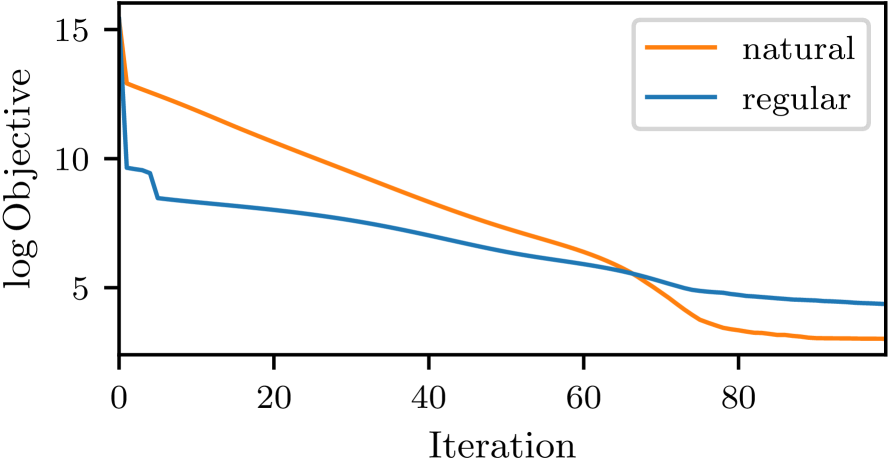
Figure 1: Evolution of the objective function under natural gradient descent (red) and regular gradient descent (blue). The lines correspond to the log of the objective function averaged over 10 runs started with randomly initialized controls.

5.2 Joint Smoothing and Inference

Geometric Brownian motion is a simple example of a process with a state dependent diffusion term and thus cannot be treated in the linear gaussian process framework. Here, we consider a simple multivariate extension given by the SDE system

$$\mathrm{d}X_{i,t}=r_{i}X_{i,t}\mathrm{d}t+X_{i,t}\mathrm{d}\tilde{W}_{i,t}$$ (24)

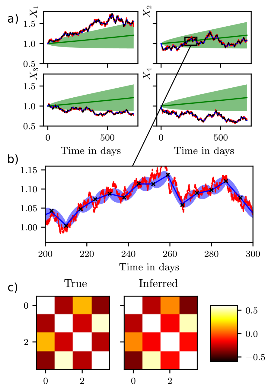
Figure 2: Joint smoothing and inference for a multivariate geometric Brownian with $n=4$. a) Noisy observations, ground truth and smoothed state for the process components. For comparison, we show the prior process initialized with uninformative parameters. The shaded region indicates the standard deviation of the prior. b) A zoom-in showing the posterior compared to the noisy observations and the ground truth. The shaded blue region indicates the standard deviation of the variational posterior. c) Ground truth of the correlation matrix compared to reconstructed correlation matrix.

for each component $i$. Here $\tilde{W}_{i,t}$ is a collection of correlated Brownian motions. Similar as for a multivariate normal distribution, a correlated Brownian motion can be constructed as $\tilde{W}_{t}=RW_{t}$ where $W_{t}$ is a vector of independent standard Brownian motions and the matrix $R$ encodes the correlations. We consider a noise-dominant scenario and thus treat $R$ as the parameter to be inferred. To test joint inference and smoothing, we simulated a trajectory over an interval of $[0,720]$ with independent Gaussian observations every $7$ units. For optimization, we use the alternating gradient descent. As demonstrated qualitatively in Fig. 2, state and correlation structure can be inferred quite well. Note that we show the correlation matrix $RR^{T}$ since many $R$ may give rise to the same process. The details of the experiment and a more quantitative evaluation are given in App. A3.1.

5.3 Amortized Smoothing

We explore the possibility of amortized smoothing (Sec. 4). To keep it simple, we consider a two-dimensional Ornstein-Uhlenbeck process given by the SDE

$$\mathrm{d}X_{t}=-\gamma(X_{t}-\mu)\mathrm{d}t+\sigma\mathrm{d}W_{t}\,.$$

where $\mu\in\mathbb{R}^{2}$, $\gamma,\sigma\in\mathbb{R}^{2\times 2}$. We generated 1000 trajectories of a two-dimensional model with fixed parameters and initial conditions. Each sample was observed over 20 $\mathrm{s}$ with 9 evenly spaced observation. The inference network was trained over 50 epochs using the Adam optimizer with default parameters, a weight decay of $0.001$ and a batch size of one. Fig. 3 shows the prediction of the smoothing network on a previously unseen sample compared to the exact solution. This demonstrates, in principle, that the controls for variational smoothing can be learned and that the inference network generalizes to unseen trajectories.

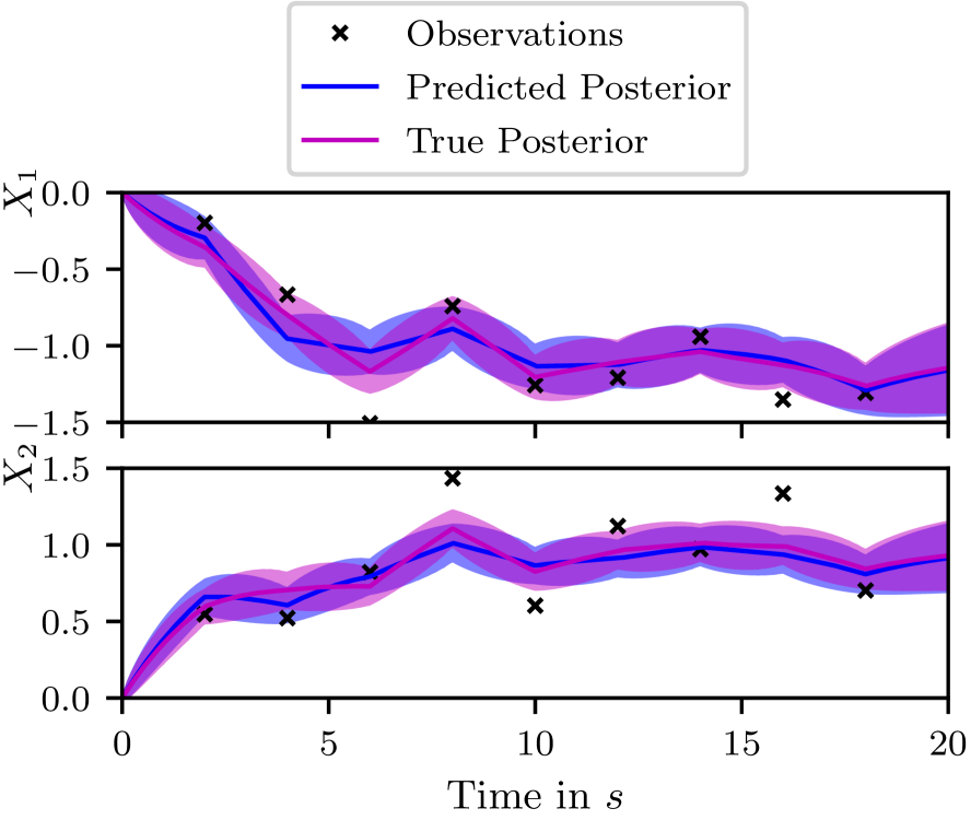
Figure 3: Two-dimensional Ornstein-Uhlenbeck process. For both components, the graph shows the smoothing predicted by the inference network on a previously unseen example. For comparison, we also show the simulated ground truth and the true posterior. Shaded regions indicate the standard deviations of the corresponding process.

5.4 Population Models

Population models describe the time evolution of a number of species over time. A convenient way to represent a population model is via the language of chemical reactions. More precisely, let there be species $\mathcal{X}_{1},\mathcal{X}_{d}$ and $r$ reactions of the form

$$s_{i1}\mathcal{X}_{1}+\ldots+s_{id}\mathcal{X}_{d}\ \xrightarrow{c_{i}}\ p_{i1}\mathcal{X}_{1}+\ldots+p_{id}\mathcal{X}_{d}$$

with the matrices $S$ and $P$ encoding the number of molecules before and after a certain reaction event and the rate constants $c_{i}$ determining the time scale of each reaction. In addition, let $V\equiv P-S$. Then the $j$-th row $v_{j}$ of $V$ encodes the net change caused by reaction $j$. Under certain conditions, the concentrations of the species is governed by the chemical Langevin equation Gillespie (2000). This leads to an SDE of the form

$$\mathrm{d}X_{t}=V^{T}h(X_{t})\mathrm{\mathrm{missing}}dt+\sqrt{V^{T}\mathrm{diag}(h(X_{t}))V}\mathrm{d}W_{t}$$ (25)

where $\sqrt{\cdot}$ indicates a matrix square root and the mass-action propensity $h:\mathbb{R}^{d}\rightarrow\mathbb{R}^{r}$ is defined component wise by

$$h_{i}(x)=c_{i}\prod_{k=1}^{d}\frac{x_{k}!}{s_{ik}!(x_{k}-s_{ik})!}.$$

We combine a linear control and a multivariate log-normal closure to derive a general method for (25) (see App. A2.4). As a test system, we use the stochastic Lotka-Volterra model that describes the interaction of a prey species and a predator species. The corresponding matrices are given by

$$S=\begin{pmatrix}1&0\\ 1&1\\ 0&1\end{pmatrix}\quad,\quad P=\begin{pmatrix}2&0\\ 0&2\\ 0&0\end{pmatrix}$$

We stress, however, that our code is not specific to the predator prey dynamics but takes general $S$ and $P$ as input. To study the behavior of our approach we recreate a scenario from Ryder et al. (2018). We generate a synthetic trajectory starting from the initial $X_{0}=(71,79)^{T}$ and take four observations within the interval $[0,50]$. As shown Fig. 4, the variational smoothing can reconstruct the true trajectory quite accurately. We also observe that only four observations restrict the variance of the process significantly.

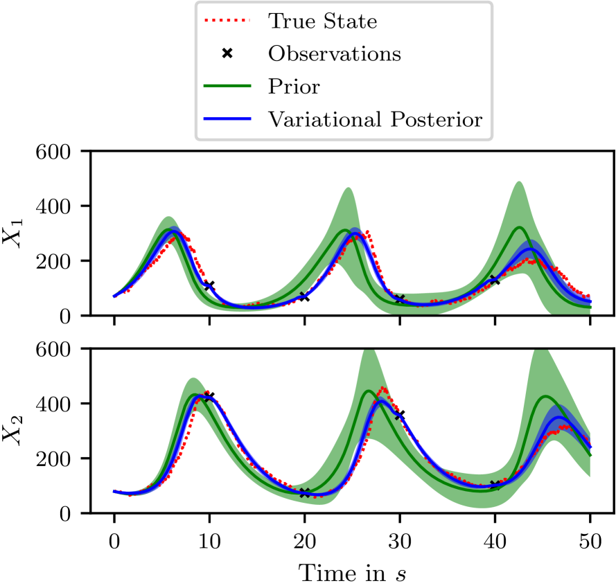
Figure 4: Smoothing for the stochastic Lotka-Volterra system. Solid lines indicate the mean, the shaded area indicates the corresponding standard deviation. Results are shown for the prior process and the variational smoothing. For reference, the simulated ground truth and the noisy observations are also provided.

6 DISCUSSION

We provide an ODE-based approach to variational smoothing that extends classical Gaussian process regression to models with state-dependent diffusion and allows for more versatile variational families. To achieve this, we understand the variational process as a controlled modification of the prior process and project the marginal posterior to a set of selected moment functions. In comparison to earlier work, we apply a refined optimization algorithm based on the natural gradient descent. Conceptually, our work extends a previous moment-based variational approach from MJPs to SDEs. Due to the structural similarity of both approaches, the moment-based variational method provides a unified inference framework for both process classes. In interesting future direction is to extend the moment-based variational framework to other Markov processes, in particular to jump-diffusions. In this work, we have used two simple closure schemes that work sufficiently well in the considered examples. Future work may consider more advanced clsoure schemes and also investigate the effect of different closures on the inference quality.
While previous ODE-based approaches have required manual derivations of the backward equation and gradients with respect to the parameters, we exploit automatic differentiation to construct these quantities automatically. In general, our approach only requires to provide two model-specific functions. For certain subclasses, these functions can be constructed automatically as well. Since our method is gradient-based, it can implemented as an automatically differentiable function. This allows straightforward integration with deep models. As a first example, we train an amortized inference network on a toy model with known model parameters. A promising future direction is to extend this to a full variational autoencoder for time series.

Appendix A1 Proofs and Derivations

A1.1 Proof of Lemma 1

Step 1

First, we derive representation (10). We start from the proposed variational drift (9) with identity rescaling, i.e.

$$a^{Z}(x,t)=a^{X}(x)+v(t)T(x)\,.$$ (A1)

with $v:[0,T]\rightarrow\mathbb{R}^{n\times m}$ and $T:\mathbb{R}^{n}\rightarrow R^{m}$. If we denote the columns of $v$ by $v_{1},\ldots,v_{m}$, the control part of Eq. (A1) may be written as

$$v(t)T(x)=\sum_{i=1}^{m}v_{i}(t)T_{i}(x)$$ (A2)

where $T_{i}$ represents the components of the vector $T$. The drift (A1) induces a family of Ito processes parametrized by the deterministic, time-dependent function $v$ given by the SDE

$$\mathrm{d}Z_{t}=\left(a^{X}(Z_{t})+v(t)T(Z_{t})\right)\mathrm{d}t+b(Z_{t})\mathrm{d}W_{t}\,.$$ (A3)

Inserting the control (A1) into the objective function (8), the prior drift $a^{X}$ cancels and the divergence between variational process and prior becomes

$$D_{\mathrm{KL}}[P^{Z}\,||\,P^{X}]=\frac{1}{2}\int_{0}^{T}\mathsf{E}\left[T(Z_{t},t)^{T}v(t)^{T}D(Z_{t},t)^{-1}v(t)T(Z_{t},t)\right]\mathrm{d}t$$ (A4)

To proceed, let us rewrite the tensor contraction within the expectation above using the expanded form of the control (A2). For clarity, we also suppress the arguments and get

$$T^{T}v^{T}D^{-1}vT=\sum_{i,j}v_{i}T_{i}D^{-1}T_{j}v_{j}$$ (A5)

Now let us define a block matrix function $\psi:\mathbb{R}^{n}\rightarrow\mathbb{R}^{nm\times nm}$ and a vector $u\in\mathbb{R}^{nm}$ as

$$\psi(x)=\begin{pmatrix}T_{1}T_{1}D^{-1}&\ldots&T_{1}T_{m}D^{-1}\\ \vdots&\cdots&\vdots\\ T_{m}T_{1}D^{-1}&\ldots,&T_{m}T_{m}D^{-1}\end{pmatrix}\,,\quad u=\begin{pmatrix}v_{1}\\ \vdots\\ v_{m}\end{pmatrix}\,.$$

With this, the tensor contraction (A5) can be written as

$$T^{T}v^{T}D^{-1}vT=u^{T}\psi u\,.$$ (A6)

Now observe that only the elements of $\psi$ depend on the stochastic process $Z_{t}$. Consequently, we arrive at the following form of the divergence

$$D_{\mathrm{KL}}[P^{Z}\,||\,P^{X}]=\frac{1}{2}\int_{0}^{T}u(t)^{T}\mathsf{E}[\psi(Z_{t})]u(t)\mathrm{d}t\,.$$ (A7)

This function contains expectations of the form $\mathsf{E}[T_{i}(Z_{t})T_{j}(Z_{t})D^{-1}_{kl}(Z_{t}))]$. By augmenting the summary statics $S$ with these quantities, we can find a function $g$ such that $\psi(t)=g(\varphi(t))$. While this choice is always possible, there may often be more convenient ways to construct $g$. Using $g$, we can write

$$D_{\mathrm{KL}}[P^{Z}\,||\,P^{X}]=\frac{1}{2}\int_{0}^{T}u(t)^{T}g(\varphi(t))u(t)\mathrm{d}t\,.$$ (A8)

as given in (10).

Step 2

What is left to show is that (A7) is a quadratic form in $u$. For this, we have to show that the matrix $\psi(t)$ is symmetric positive semi-definite for almost every $t\in[0,T]$. The function $\psi$ is symmetric by construction. Consequently, $E[\psi(Z_{t})]$ is symmetric. Now fix $u\in\mathbb{R}^{nm}$ and let $v$ be the corresponding matrix representation. Set

$$H(v,t)=T(x,t)^{T}v(t)^{T}D^{-1}(x,t)v(t)T(x,t)\,.$$

Then $H(v,t)\geq 0$ for almost all $x\in\mathbb{R}^{n}$ and $t\in[0,t]$. To see this, we understand $v(t)T(x,t)$ as a vector in $\mathbb{R}^{n}$. The result follows because $D(x,t)$ is p.s.d. almost everywhere by assumption. Here, the strict definiteness is lost in general. For example, if $m>n$ we may find $v$ such that $v(t)T(x,t)=0$. Now since $H$ and $A$ represent the same quadratic form, $A$ has to be positive semi-definite as well.

Step 3

So far, we have not considered rescaling. Now let $R:\mathbb{R}^{n}\rightarrow R^{n\times n}$ be an invertible matrix valued function and consider the rescaled controlled drift

$$a^{Z}(x,t)=a^{X}(x)+R(x)v(t)T(x,t)\,.$$

Evaluating the prior contribution to the divergence yields

$$D_{\mathrm{KL}}[P^{Z}\,||\,P^{X}]=\frac{1}{2}\int_{0}^{T}\mathsf{E}\left[T(Z_{t})^{T}v(t)^{T}\underbrace{R(Z_{t})^{T}D(Z_{t},t)^{-1}R(Z_{t})}_{\equiv\tilde{D}^{-1}(Z_{t})}v(t)T(Z_{t})\right]\mathrm{d}t\,.$$ (A9)

We can now directly repeat steps 1 and 2 by replacing $D(x)\rightarrow\tilde{D}(x)$ in the construction of $g$.

A1.2 Proof of Proposition 1

The full variational inference problem for the proposal class parametrized by $u$ is given by

$$\min_{u}\frac{1}{2}\int_{0}^{T}u(t)^{T}g(\varphi(t))u(t)\,\mathrm{d}t-\sum_{k=1}^{n}\mathsf{E}[\log p(y_{k}\mid Z_{t_{k}})]+\log C\,.$$ (A10)

Eq. (A10) is a direct consequence of (8) and Lemma 1 and may be understood as a stochastic control problem. We now assume that the expected log-likelihood may be expressed in terms of the expected summary statistics $\varphi$, i.e. $\mathsf{E}[\log p(y_{k}\mid Z_{t_{k}})]=F(\varphi(t_{k}))$ . We also ignore the evidence $\log C$ which is independent of $u$. This leads to the streamlined representation

$$\min_{u}\frac{1}{2}\int_{0}^{T}u(t)^{T}g(\varphi(t))u(t)\,\mathrm{d}t-\sum_{k=1}^{n}F(\varphi(t_{k}))\,.$$ (A11)

The objective function in (A11) corresponds to the negative ELBO for the proposal family parametrized by $u$. Unfortunately, the simple appearance of (A11) is deceiving since $\varphi(t)=\mathsf{E}[S(Z_{t})]$ implicitly depends on $u$. Now recall that $\varphi(t)$ obeys an evolution equation of the form

$$\frac{d}{dt}\varphi(t)=\mathsf{E}[A^{\dagger}S(Z_{t})]\,.$$

We can now convert (A11) into a constrained problem

$$\begin{aligned} \min_{u,\varphi}&&&\frac{1}{2}\int_{0}^{T}u(t)^{T}g(\varphi(t))u(t)\,\mathrm{d}t-\sum_{k=1}^{n}F_{i}(\varphi(t_{k}))\\ \mathrm{s.t.}&&&\dot{\varphi}(t)=\mathsf{E}[A^{\dagger}S(Z_{t})]\,\\ \end{aligned}\,.$$ (A12)

We emphasize that (A12) is an equivalent representation of the variational problem and does not contain any approximations beyond the choice of the variational family. This also means that it has the full complexity of the original stochastic control problem (A10). In order to obtain a more tractable problem, we use a moment closure on the constraint to get an ODE of the form

$$\frac{d}{dt}\varphi(t)=f(u,\varphi(t))\,.$$ (A13)

With this moment closure relaxation, the variational problem (A12) reduces to the deterministic control problem given in the main text.

Comment

In general, when a moment closure is employed, there is no global Markov process corresponding exactly to the closed moment equations. Then, the objective function is not a true lower bound of the evidence but an approximate lower bound. Such behavior is well-known for other structured variational approximation, e.g. for cluster variational methods Yedidia et al. (2000); Wainwright and Jordan (2008). Since moment closure introduces an additional approximation, results of the moment-based variational inference have to be checked empirically. However, we do not see this as a major problem since such empirical verification is required for all forms of variational inference anyway.

A1.3 Proof of Lemma 2

Consider to stochastic processes $Z$ and $Z^{\prime}$ over an interval $[0,T]$ that are members of the variational family as defined by the drift and Eq. (9). Let $Z$ and $Z^{\prime}$ be parametrized by $u$ and $u^{\prime}$, respectively. Inserting $Z$ and $Z^{\prime}$ into the general path divergence of diffusion processes (7) , we get

$$D_{\mathrm{KL}}[Z\,||\,Z^{\prime}]=\frac{1}{2}\int_{0}^{T}\mathsf{E}\left[T(Z_{t})^{T}\left(v^{\prime}(t)-v(t)\right)^{T}D^{-1}(Z_{t},t)\left(v^{\prime}(t)-v(t)\right)T(Z_{t})\right]dt$$

This expression is the same as (A4) with $v$ replaced by $v-v^{\prime}$. Therefore, we may follow along the same lines as in Sec. A1.1 and obtain

$$D_{\mathrm{KL}}[Z\,||\,Z^{\prime}]=\frac{1}{2}\int_{0}^{T}\left(u^{\prime}(t)-u(t)\right)^{T}g(\varphi(t))\left(u^{\prime}(t)-u\right)dt\,.$$

To get the suggested representation, set $G:\mathcal{U}\times\mathcal{U}\rightarrow\mathbb{R}$ as

$$G(u)[u^{\prime}-u,u^{\prime}-u]=\int_{0}^{T}\left(u^{\prime}(t)-u(t)\right)^{T}g(\varphi(t))\left(u^{\prime}(t)-u\right)dt\,.$$

What is left is to verify the properties of $G$. Bilinearity follows immediately from the above definition. The symmetry and positive definiteness follow from Lemma 1.

A1.4 Proof of Proposition 2

Consider the variational problem of the main text given by

$$u^{*}=\arg\min_{u}J[u]\,.$$ (A14)

Here, we understand $J$ as a functional of the controls $u$ only. This is possible because $u$ together with an initial condition fully defines the moments $\varphi$. We would like to perform a steepest descent that respects the metric of the manifold on which $u$ lives. We therefore replace (A14) by the sequential optimization problem

$$u^{(i+1)}=\arg\min_{u}J[u]\,,\quad\mathrm{s.t.}\quad\frac{1}{2}G(u^{(i)})(u-u^{(i)},u-u^{(i)})=\epsilon\,.$$

The following calculation is inspired by the discussion of neighboring optimal solutions in Stengel (1994). For sufficiently small $\epsilon$, we may linearize $J$ around the current estimate $u^{(i)}$. Enforcing the constraint via a Lagrange multiplier, we obtain the unconstrained functional

$$J^{\prime}[u,\lambda]=J[u^{(i)}]+\delta J[u^{(i)},u-u^{(i)}]+\lambda\left(\frac{1}{2}G(u^{(i)})(u-u^{(i)},u-u^{(i)})-\epsilon\right)\,.$$

Here $\delta J$ denotes the Gateaux derivative of $J$. For simplicity, set $\delta u=u-u^{(i)}$. We consider $\delta u$ as a small perturbation of $u^{(i)}$ and denote as $\delta\varphi$ the deviation from $\varphi^{(i)}$ induced by $\delta u$. It turns out that $\delta\varphi$ satisfies the linearized forward equation

$$\dot{\delta\varphi(t)}=f_{\varphi}(u^{(i)}(t),\varphi^{(i)}(t))\delta\varphi(t)+f_{u}(u^{(i)}(t),\varphi^{(i)}(t))\delta u\,.$$ (A15)

The linearized contribution $\delta J$ is given by

$$\delta J[u^{(i)},u-u^{(i)}]=\int_{0}^{T}L_{\varphi}(u^{(i)}(t),\varphi^{(i)}(t))\delta\varphi(t)\mathrm{d}t+\int_{0}^{T}L_{u}(u^{(i)}(t),\varphi^{(i)}(t))\delta u(t)\mathrm{d}t\,$$

where $\varphi$ is understood as a function of $\delta u$ determined by (A15). We therefore obtain the objective function

$$\begin{split}J^{\prime}[u,\lambda]&=\int_{0}^{T}L_{\varphi}(u^{(i)}(t),\varphi^{(i)}(t))\delta\varphi(t)\mathrm{d}t+\int_{0}^{T}L_{u}(u^{(i)}(t),\varphi^{(i)}(t))\delta u(t)\mathrm{d}t\\ &\quad+\frac{\lambda}{2}\int_{0}^{T}\delta u(t)^{T}\psi(\varphi^{(i)}(t))\delta u(t)\mathrm{d}t+\mathrm{const}\,.\end{split}$$ (A16)

that we have to minimize subject to the constraint (A15). We can now follow the standard variational procedure to obtain an adjoint equation

$$\dot{\eta}(t)=L_{\varphi}(u^{(i)}(t),\varphi^{(i)}(t))-f_{\varphi}^{T}(u^{(i)}(t),\varphi^{(i)}(t))\eta(t)$$ (A17)

that satisfies the reset conditions

$$\eta(t_{k}^{-})=\eta(t_{k}^{+})+\frac{d}{d\varphi}F(\varphi(t_{k})),\quad k=1,\ldots,n$$ (A18)

at the observation times. In addition, we obtain the algebraic constraint

$$0=L_{u}(u^{(i)}(t),\varphi^{(i)}(t))-f_{u}(u^{(i)}(t),\varphi^{(i)}(t))\eta(t)+\lambda\psi(\varphi^{(i)}(t))\delta u(t)\,.$$ (A19)

In contrast to the non-linearized problem, the stationarity conditions decouple in this case. This means we can solve for the controls explicitly. Denoting the solution of (A17) as $\eta^{(i)}$ the solution can be expressed as

$$\delta u^{(i)}(t)=-\frac{1}{\lambda}g^{-1}(\varphi^{(i)}(t))\left(L_{u}(u^{(i)}(t),\varphi^{(i)}(t))-f_{u}(u^{(i)}(t),\varphi^{(i)}(t))\eta^{(i)}(t)\right)$$ (A20)

Now we also know that $L_{u}(u^{(i)}(t),\varphi^{(i)}(t))=g(\varphi^{(i)}(t))u^{(i}(t)$. Thus, we get the natural gradient update steps as

$$u^{(i+1)}(t)=u^{(i)}(t)+\delta u^{(i)}(t)=u^{(i)}(t)-h\left(u^{(i)}(t)-\psi^{-1}(\varphi^{(i)}(t))f_{u}(u^{(i)}(t),\varphi^{(i)}(t))\eta^{(i)}(t)\right)\,.$$ (A21)

Here, we also introduced the step size $h=\frac{1}{\lambda}$ that is determined by $\epsilon$. To recover the regular gradient, we use that gradient descent is a steepest descent with respect to the Euclidean metric. In our function space setting, the natural analogue is the $L_{2}$ norm. Therefore, gradient descent is obtained by repeating the above calculations for

$$G(u)(u^{\prime}-u,u^{\prime}-u)=\int_{0}^{T}(u^{\prime}(t)-u(t))^{T}(u^{\prime}(t)-u(t))\,\mathrm{dt}\,.$$

Thus, the only thing we have to change is replacing $g^{-1}$ in (A20) with the identity matrix.

Comments

In a typical application, we will initialize the descent with all controls set to zero. This setting recovers the prior process. Intuitively, we can see the natural gradient descent as a smooth transition from the prior process to the (locally) best posterior approximation within the variational family. We note that due to moment closure, we only have access to approximate moments $\varphi$. Therefore, the natural gradient is also an approximation to the true natural gradient.

A1.5 Recovering the Gaussian Process Approximation

For this section, we assume that the diffusion term $b$ does not depend on the state. The Gaussian process approximation only requires first and second order moments. We therefore choose

$$S(x)=(x_{1},\ldots,x_{n},x_{1}^{2},x_{1}x_{2},x_{2}^{2},\ldots,x_{n}^{2})^{T}\,.$$

The GP approximation is defined by a linear time-dependent drift. In order to recover this within our framework, we need to find $T$ such that

$$a^{Z}(x,t)=a(x)+v(t)T(x)\stackrel{{\scriptstyle!}}{{=}}u_{0}(t)+u_{1}(t)x$$

where $u_{0}:[0,T]\rightarrow\mathbb{R}^{n}$ and $u_{1}:[0,T]\rightarrow\mathbb{R}^{n\times n}$. Now consider the choice

$$T(x,t)=\begin{pmatrix}1\\ x\\ a(x,t)\end{pmatrix}\,,\quad v(t)=\begin{pmatrix}u_{0}(t)&u_{1}(t)&u_{2}(t)\end{pmatrix}$$

understood as block matrix notation with $u_{2}:[0,T]\rightarrow\mathbb{R}^{n\times n}$. This will lead to a variational drift of the form

$$a^{Z}(x,t)=a(x)+u_{0}(t)+u_{1}(t)x+u_{2}(t)a(x)\,.$$

If we fix $u_{2}$ to the constant function with output minus one, the prior drift will cancel and we have constructed a linear GP. Using the general moment equation (2) with the drift $a^{Z}$, we can now derive the moment equations for $\varphi(t)=\mathsf{E}[S(Z_{t})]$. Represented in terms represented in terms of $m$, $\bar{M}$ we get

$$\begin{split}\dot{m}(t)&=u_{0}(t)+u_{1}(t)m(t)\,,\\ \dot{\bar{M}}(t)&=u_{1}(t)\bar{M}(t)+\bar{M}(t)u_{1}(t)^{T}+D\,.\end{split}$$ (A22)

These equations are the standard equations for mean and variance of a linear GP. Eq. (A22) defines the forward function $f$ required for implementation in our framework. The second function required is $L$ or $g$. Here, $L$ is a bit more convenient and is given by

$$L(u(t),\varphi(t))=\mathsf{E}[(u_{0}(t)+u_{1}(t)x-a(Z_{t}))^{T}D^{-1}(u_{0}(t)+u_{1}(t)Z_{t}-a(Z_{t}))]\,.$$

After a few algebraic multiplications, we observe that the only model dependent quantities required for $L$ are $\mathsf{E}[a(Z_{t}]$, $\mathsf{E}[a(Z_{t})Z_{t}^{T}]$ and $\mathsf{E}[a(Z_{t})a(Z_{t})^{T}]$ expressed as functions of $m$ and $\bar{M}$.

Appendix A2 Additional Information

A2.1 Moment Closure Approximations

In the main part, we discussed how two obtain moment equations for Markov processes and gave a general idea on moment closure. Here, we will discuss strategies to obtain such a closure scheme, i.e. how to find the function $h$ such that we can proceed from (4) to (5). We focus on distributional closures that correspond to a projection onto a given parametric family (Bronstein and Koeppl, 2018). A distributional closure is constructed by picking a parametric proposal distribution $q_{\phi}$ on the state space $\mathcal{X}$. To obtain a closure scheme, the first step is to find $\phi(t)$ such that

$$\mathsf{E}_{\phi(t)}[R(X)]=\varphi(t)\,,$$ (A23)

where $\varphi(t)=\mathsf{E}[S(Z_{t})]$ are the expected summary statistics used to approximate the process. Eq. (A23) defines a valid moment closure when the conditions of the implicit function theorem are satisfied. Assuming we have obtained $\varphi(t)$, we can evaluate

$$h(\varphi(t))\equiv\mathsf{E}_{\phi(t)}[R(X)]\,,$$ (A24)

where the expectation is taken with respect to $q_{\phi(t)}$.

It has also been shown that moment closure tends to work better if the support of the proposal distribution matches the support of the target process. Here, we focus on two simple probabilistic closures: the multivariate normal closure for processes defined on $\mathbb{R}^{n}$ and the multivariate log-normal closure for processes defined on $\mathbb{R}_{+}^{n}$. Another advantage of these two schemes is that they correspond directly to first and second order moments and may thus be used as a starting point before investigating more advanced schemes. To simplify the presentation, we denote the first order moments as $m\equiv\mathsf{E}[X]$, the second order moments as $M\equiv\mathsf{E}[XX^{T}]$ and the second order central moments as $\bar{M}\equiv\mathsf{E}[(X-m)(X-m)^{T}]$. We write general powers in multi-index form, i.e.

$$X^{\alpha}\equiv\prod_{i=1}^{n}X_{i}^{\alpha_{i}}\,.$$

This will be useful to represent general power moments. We also define $k\equiv\sum_{i=1}^{n}\alpha_{i}$ as the order of the $\alpha$-th multi-moment.

Multivariate Normal Clouse

Let $X\sim\mathcal{N}(\mu,\Sigma)$ be a multivariate normal random variable on $\mathbb{R}^{n}$. Since the distribution is fully specified by the man $\mu$ and the covariance $\Sigma$, all moments of the form $\mathsf{E}[X^{\alpha}]$ with $\alpha\in\mathbb{N}^{n}$ can be expressed as functions of $\mu$ and $\Sigma$. One way to obtain such a representation is via Isserlis’ theorem (Isserlis, 1918). We will follow an alternative approach via the moment generating function.

Lemma A1.

Let $X$ be as above and $\alpha\in\mathbb{R}^{n}$ a multi-index. Then

$$\mathsf{E}[X^{\alpha}]=\left.\prod_{i=1}^{n}\frac{\partial^{\alpha_{i}}}{\partial s_{i}^{\alpha_{i}}}M(s)\right|_{s=0}$$

where

$$M(s)=\mathsf{E}[\exp(s^{T}X)]=\exp\left(\mu^{T}s+\frac{1}{2}s^{t}\Sigma s\right)$$

is the moment generating function of $\mathcal{N}(\mu,\Sigma)$.

While Lemma (A1) does not provide an explicit formula for direct numerical implementation, it is straightforward to automatically generate the closure relations using a computer algebra system. In particular, we automatically construct moment equations using Sympy (Meurer et al., 2017) and convert them to PyTorch functions.

Multivariate Lognormal Closure

A log-normal random variable can be obtained by exponential transform of a normal random variable. This generalizes to the multivariate case. More specifically, let $Z\sim\mathcal{N}(\mu,\Sigma)$. Then we say

$$X=\exp(Z)\,$$

has a log-normal distribution. Here, the exponential is understood as acting component-wise.

Lemma A2.

Let $X$ be as above and $\alpha\in\mathbb{R}^{n}$ a multi-index. Then

$$\mathsf{E}[X^{\alpha}] =\left(\prod_{i}\frac{\mathsf{E}[X_{i}]^{2\alpha_{i}}}{\mathsf{E}[X_{i}^{2}]^{\frac{\alpha_{i}}{2}}}\right)\left(\prod_{i,j}\frac{\mathsf{E}[X_{i}X_{j}]^{\frac{\alpha_{i}\alpha_{j}}{2}}}{\mathsf{E}[X_{i}]^{\frac{\alpha_{i}\alpha_{j}}{2}}\mathsf{E}[X_{j}]^{\frac{\alpha_{i}\alpha_{j}}{2}}}\right)\,$$

This result can be shown by exploiting that $\mathsf{E}[X^{\alpha}]=\mathsf{E}\left[\exp\left(\alpha^{T}Z\right)\right]$ corresponds to the moment generating function of a normal distribution. As a consequence of Lemma A2, we obtain the explicit closure function

$$\mathrm{Cl}(m,M,\alpha)=\left(\prod_{i}\frac{m_{i}^{2\alpha_{i}}}{M_{i}^{\frac{\alpha_{i}}{2}}}\right)\left(\prod_{i,j}\frac{M_{ij}^{\frac{\alpha_{i}\alpha_{j}}{2}}}{m_{i}^{\frac{\alpha_{i}\alpha_{j}}{2}}m_{j}^{\frac{\alpha_{i}\alpha_{j}}{2}}}\right)\,.$$ (A25)

The log-normal closure (A25) can be implemented efficiently using tensor operations. It is also differentiable and thus suitable for backpropagation.

A2.2 Rescaling

Consider a drift without rescaling of the form (A1). While leading to a convenient quadratic objective function, this form of the control has two major drawbacks. The first drawback is that the matrix-valued function $g$ in (10) is of dimension $(n\cdot m,n\cdot m)$ with $n$, $m$ corresponding to the dimension of the state space and the number of control features, respectively. Assuming the number control features is proportional to the dimension, the function $g$ requires $\mathcal{O}(n^{4})$ elements. The second problem is specific to models with state-dependent diffusion term. In this case, the elements of $g$ are of the form $\mathsf{E}[T_{i}(Z_{t})T_{j}(Z_{t})D^{-1}_{kl}(Z_{t})]$. This expression requires an analytic inverse of the diffusion tensor which is rarely available. We now discuss two special choices of rescaling. First, consider a case where the diffusion term $b$ is known analytically and set $R=b$. We then have

$$\tilde{D}^{-}1(x)\equiv b(x)^{T}D^{-1}(x)b(x)=b(x)^{T}\left(b(x)b(x)^{T}\right)^{-1}b(x)=I\,.$$

The matrix $g$ now only depends on moments of the form $\mathsf{E}[T_{i}(Z_{t},t)T_{j}(Z_{t},t)]$. As a consequence, the objective function becomes independent of the diffusion tensor. In addition, the number of non-zero elements of $g$ now scales as $\mathcal{O}(n^{2})$. The second choice of rescaling aims at the case where we are provided with $D$ rather than $b$ and thus consider $R=D$ leading to

$$\tilde{D}^{-1}(x)=D(x)^{T}D^{-1}(x)D(x)=D(x,t)\,.$$ (A26)

While this choice does not improve the scaling, $g$ now depends on expressions of the form $\mathsf{E}[T_{i}(Z_{t})T_{j}(Z_{t})D_{kl}(Z_{t})]$ such that we get rid of the inverse diffusion tensor. It also has an interesting intuitive interpretation. Recall that the true posterior drift is given by $\bar{a}(x,t)=a(x,t)+D(x,t)\nabla\log(\beta(x,t))$. Thus, the ansatz corresponds to approximating the log-transformed backward function by a linear feature model.

A2.3 A Standard Approximation

Inspired by the variational Gaussian process approximation, we would like to construct a method that approximates the data-driven term by a feedback control linear in the state and requires first and second order moments. This corresponds to the choices

$$\begin{split}S(x)&=(x_{1},\ldots,x_{n},x_{1}^{2},x_{1}x_{2},x_{2}^{2},\ldots,x_{n}^{2})^{T}\,,\\ T(x)&=(1,x_{1},\ldots,x_{n})^{T}\,.\end{split}$$

For this special class, it is convenient to represent the control in terms of functions $u_{0}$, $u_{1}$ such that we can write

$$v(t)T(x)=u_{0}(t)+u_{1}(t)x$$ (A27)

A short calculation shows that the moment equations are given by

$$\begin{split}\dot{m}(t)&=\mathsf{E}[a(Z_{t})]+\mathsf{E}[R(Z_{t})]u_{0}(t)+\mathsf{E}(R(Z_{t})u_{1}(t)Z_{t}]\\ \dot{M}(t)&=E[a(Z_{t})Z_{t}^{T}]+E[Z_{t}a(Z_{t})^{T}]+\mathsf{E}[D(Z_{t})]\\ &\quad+\mathsf{E}[R(Z_{t})u_{0}Z_{t}^{T}]+\mathsf{E}[Z_{t}u_{0}Z_{t}^{T}R(Z_{t})^{T}]\\ &\quad+\mathsf{E}[R(Z_{t})u_{1}(t)Z_{t}Z_{t}^{T}]+\mathsf{E}[Z_{t}Z_{t}^{T}u_{1}(t)^{T}R(Z_{t})^{T}]\end{split}$$

A2.4 Specific Subclasses

In this section, we present moment equations for special classes and more specific models considered in the experiment section.

Constant Diffusion

For models with constant diffusion terms $b$, we can always choose the corresponding rescaling. In combination with the approach outlined in A2.3, we obtain the moment equations

$$\begin{split}\dot{m}(t)&=\mathsf{E}[a(Z_{t})]+bu_{0}(t)+bu_{1}(t)m(t)]\,,\\ \dot{M}(t)&=E[a(Z_{t})Z_{t}^{T}]+E[Z_{t}a(Z_{t})^{T}]+bb^{T}\\ &\quad+bu_{0}(t)m(t)^{T}+m(t)u_{0}(t)^{T}b^{T}+bu_{1}(t)M(t)+M(t)u_{1}(t)^{T}b^{T}\,.\end{split}$$

The second function required is the contribution to the KL-divergence that can be provided in terms of $L$ or $g$ (c.f. Thm. 1). Here, using $L$ is more convenient and we get

$$L(u(t),m(t),M(t))=\frac{1}{2}\left(u_{0}(t)^{T}u_{0}(t)+2u_{0}(t)^{T}u_{1}(t)m(t)+\mathrm{Tr}(u_{1}(t)^{T}u_{1}(t)M(t))\right)\,.$$

Since the last equation is model-independent, we have implemented a base class from which custom models can be derived. In particular, implementation of a given model only requires custom functions for $\mathsf{E}[a(Z_{t})]$ and $E[a(Z_{t})Z_{t}^{T}]$. For polynomial drift functions, the required expectations can be evaluated straightforwardly using our Gaussian moment closure implementation in Sympy (c.f. Lemma A1).

Population Models

We consider a general population model defined by the chemical Langevin equation (25). Here, the diffusion term $b(x)$ is not given and we have only access to the diffusion tensor $D(x)=V^{T}\mathrm{diag}(h(X_{t}))V$. We will therefore choose a linear control with rescaling $R=D$. In the regime where the CLE is valid, we typically have $X_{i}\gg 1$. We will also restrict the discussion to physically plausible systems with $s_{ik}\leq 2$. Under these conditions, the propensity functions can be approximated as

$$h_{i}(x)=c_{i}\prod_{k=1}^{d}x_{k}^{s_{ik}}\,.$$ (A28)

For the proposed variational process class, we obtain the moment equations

$$\begin{split}m_{i}(t)&=V_{ji}\mathsf{E}[h_{j}(Z_{t})]+V_{ki}V_{kj}u_{0,j}(t)\mathsf{E}[h_{k}(Z_{t})]+V_{li}V_{lj}u_{1,jk}(t)\mathsf{E}[h_{l}(Z_{t})Z_{t,k}]\\ M_{ij}(t)&=V_{ki}\mathsf{E}[h_{k}(Z_{t})Z_{t,j}]+V_{kj}\mathsf{E}[h_{k}(Z_{t})Z_{t,i}]+V_{ki}V_{kl}u_{0,l}(t)\mathsf{E}[h_{k}(Z_{t})Z_{t,j}]+V_{kj}V_{kl}u_{0,l}(t)\mathsf{E}[h_{k}(Z_{t})Z_{t,i}]\\ &\quad+V_{ki}V_{kl}u_{1,lm}(t)\mathsf{E}[h_{k}(Z_{t})Z_{t,m}Z_{t,j}]+V_{kj}V_{kl}u_{1,lm}(t)\mathsf{E}[h_{k}(Z_{t})Z_{t,m}Z_{t,i}]+V_{ki}V_{kj}\mathsf{E}[h_{k}(Z_{t})]\end{split}$$ (A29)

While these expressions may look unwieldy, we observe that when the propensities are modeled by (A28), all expectations in (A28) are of the form $\mathsf{E}[Z_{t}^{\alpha}]$ and can be easily evaluated with the generic log-normal closure function A25. In addition, expectations required for the function $g$ are of the same form.

Multivariate Geometric Brownian Motion

For the multivariate Brownian motion model described in the main text, we consider a linear control with rescaling $b$. We obtain the moment equations

$$\begin{split}\dot{m}_{i}(t)&=r_{i}m_{i}(t)+m_{i}(t)R_{ij}u_{0,j}(t)+R_{ij}u_{1,jk}M_{ik}(t)\,,\\ \dot{M}_{ij}&=r_{i}M_{ij}(t)+r_{j}M_{ji}(t)+R_{ik}u_{0,k}M_{ij}(t)+R_{jk}u_{0,k}M_{ji}(t)\\ &\quad+R_{ik}u_{1,kl}\mathsf{E}[Z_{t,i}Z_{t,j}Z_{t,l}]+R_{jk}u_{1,kl}\mathsf{E}[Z_{t,i}Z_{t,j}Z_{t,l}]+D_{ij}M_{ij}(t)\end{split}$$ (A30)

where we have used Einstein sum convention. In order to obtain closed equations, we compute the third order moments $E[Z_{t,i}Z_{t,j}Z_{t,l}]$ via the general log-normal closure formula given in Lemma A2. Since for the rescaling with $b$, the second function $g$ becomes independent of the model, (A30) is the only model specific quantity required for implementation.

A2.5 Parameter Inference

A2.5.1 Extended Control Problem

Variational parameter inference corresponds to maximizing the evidence lower bound jointly with respect to the model parameters $\theta$ and variational parameters $u$. If we instead minimize the negative ELBO, we obtain the optimization problem

$$\min_{\theta,u}\quad\underbrace{D_{\mathrm{KL}}[P^{Z}\,||\,P^{X}]-\sum_{k=1}^{n}\mathsf{E}[\log p(y_{k}\mid Z_{t_{k}})]}_{\equiv J[\theta,u]}\,.$$ (A31)

We can now do the same reductions as for the derivation of the smoothing control problem

$$\begin{aligned} \min_{\theta,u,\varphi}&&&\frac{1}{2}\int_{0}^{T}u(t)^{T}g(\theta,\varphi(t))u(t)\,\mathrm{d}t-\sum_{k=1}^{n}F_{i}(\varphi(t_{k}))\\ \mathrm{s.t.}&&&\dot{\varphi}(t)=\mathsf{E}[A^{\dagger}S(Z_{t})]\,\\ \end{aligned}\,.$$ (A32)

Of course, the dynamic constraint depends on $\theta$ as well. Three methods are commonly used to solve the variational inference problem (A31).

Coordinate Descent

Starting from an initial guess $\theta^{(0)}$, $u^{(0)}$ the updates are computed as

$$u^{(i+1)} =\min_{u}J[\theta^{(i)},u]\,,$$

$$\theta^{(i+1)} =\min_{\theta}J[\theta,u^{(i+1)}]\,.$$

This is the classical variational expectation maximization(VEM) algorithm used in mean field variational inference. It is most effective when the updates can be computed in closed form. In the scenario considered here, this will typically not be the case. Even if possible, obtaining the closed form updates requires model specific calculations that we try to avoid. We therefore do not consider the VEM any further.

Gradient Descent

In Prop. 2, we have presented regular and natural gradient descent in the controls to solve the smoothing problem. The proof can be extended straightforwardly to include a gradient update with respect to $\theta$ as well. More explicitly, the parameter updates take the form

$$\theta^{(i+1)}=\theta^{(i)}-h\int_{0}^{T}\left(L_{\theta}(\theta^{(i)},u^{(i)}(t),\varphi^{(i)}(t))-f_{\theta}(\theta^{(i)},u^{(i)}(t),\varphi^{(i)}(t))\eta^{(i)}(t)\right)\mathrm{d}t\,$$ (A33)

with notational conventions as in Prop. 2. Eq. (A33) corresponds to a regular gradient and can be evaluated without model specific derivations based on automatic differentiation.

Alternating Gradient Descent

A third alternative is to iteratively take a number of gradient steps for the $u$ and $\theta$ while keeping the other fixed (see Algorithm 2). This method has two main advantages over the full gradient descent. First, we can use separate step sizes for the model and variational parameter updates. Second, since $\theta$ is fixed for the descent in $u$, we can still exploit the natural gradient for the latter. The alternating gradient descent can be seen as a hybrid between VEM and gradient descent. This is because if we performed every inner gradient descent up to convergence, the result would be equivalent to the VEM updates.

Algorithm 2 Robust Alternating Gradient Descent for Moment-Based Variational Inference

1:  Input: Initial guesses $\theta^{(0)}$, $u^{(0)}$, initial condition $\varphi(0)$, learning rates $h_{0},h_{1}$.

2:  for  $i=0,\ldots,i_{\mathrm{max}}$ do

3:     $u^{(i,0)}\rightarrow u^{(i)}$

4:     for $k=0,\ldots,k_{\mathrm{max}}$  do

5:        Set $u^{\prime}$ according to (A21).

6:        if  $J[\theta^{(i)},u^{\prime}]<J[\theta^{(i)},u^{(i,k)}]$  then

7:           $h_{0}\rightarrow\alpha\cdot h_{0}$, $u^{(i,k+1)}\rightarrow u^{\prime}$

8:        else

9:           $h_{0}\rightarrow\beta\cdot h_{0}$, $u^{(i,k+1)}\rightarrow u^{(i,k)}$

10:        end if

11:     end for

12:     $u^{(i+1)}\rightarrow u^{(i,k_{\mathrm{max}})}$

13:     $\theta^{(i,0)}\rightarrow\theta^{(i)}$

14:     for  $k=0,\ldots,k_{\mathrm{max}}$  do

15:        Set $\theta^{\prime}$ according to (A33).

16:        if  $J[\theta^{\prime},u^{(i+1)}]<J[\theta^{(i,k)},u^{(i+1)}]$  then

17:           $h_{1}\rightarrow\alpha\cdot h_{1}$, $\theta^{(i,k+1)}\rightarrow\theta^{\prime}$

18:        else

19:           $h_{1}\rightarrow\beta\cdot h_{1}$, $\theta^{(i,k+1)}\rightarrow\theta^{(i,k)}$

20:        end if

21:     end for

22:     $\theta^{(i+1)}\rightarrow\theta^{(i,k_{\mathrm{max}})}$

23:  end for

24:  Output: $\theta^{(i_{\mathrm{max}})}$, $u^{(i_{\mathrm{max}})}$

A2.5.2 Amortized Inference

In many scenarios ones observes not a single trajectory but a number of trajectories $\mathbf{x}_{1},\ldots,\mathbf{x}_{n}$ produced independently from the same model underlying model with parameter $\theta$. Denote the corresponding noisy observations as $\mathbf{y}_{1},\ldots,\mathbf{y}_{N}$. We use boldface to indicate that $\mathbf{x}_{i}$, $\mathbf{y}_{i}$ corresponds to trajectories of stochastic processes. However, to keep the following discussion simple, we will treat them informally as ordinary random variables. Thus, the joint data likelihood is given by

$$p(\mathbf{y}_{1},\ldots,\mathbf{y}_{n}\mid\theta)=\prod_{i=1}^{N}p_{i}(\mathbf{y}_{i}\mid\theta)=\prod_{i=1}^{N}\int p_{i}(\mathbf{y}_{i}\mid\mathbf{x}_{i})p_{i}(\mathbf{x}_{i}\mid\theta)\mathrm{d}\mathbf{x}_{i}\ \,$$

where $\mathbf{x}_{i}$ corresponds to the trajectory of the latent diffusion process in this case. The standard VI approach is to construct an evidence lower bound based on the proposal

$$q(\mathbf{x}_{1},\ldots\mathbf{x}_{n})=\prod_{i=1}^{n}q_{i}(\mathbf{x}_{i}\mid u_{i})\,.$$

In our case, every $q_{i}$ corresponds to a full stochastic process $Z_{i}$ parametrized by $u_{i}$ with $u_{i}$ being a function of time. Consequently, the joint variational inference problem becomes infeasible very quickly due to large memory and runtime requirements. We therefore use an amortized proposal of the form

$$q(\mathbf{x}_{1},\ldots\mathbf{x}_{n})=\prod_{i=1}^{n}q_{i}(\mathbf{x}_{i}\mid h(y_{i},\phi))$$

where $h$ is a feed-forward neural network parametrized by $\phi$. The corresponding ELBO is given by

$$\mathrm{ELBO}(\theta,\phi)=\sum_{i=1}^{N}\int q_{i}(\mathbf{x}_{i}\mid h(\mathbf{y}_{i},\phi))\log p(\mathbf{y}_{i}\mid\mathbf{x}_{i})-D_{\mathrm{KL}}[q_{i}\,||\,p_{i}]\,.$$ (A34)

Now observe that every term in the sum above corresponds the objective function of the variational inference problem for a single trajectory. We may thus write

$$-\mathrm{ELBO}(\theta,\phi)=\sum_{i=1}^{N}J[\theta,h(\mathbf{y}_{i},\phi)]$$ (A35)

with $J[\theta,u]$ as defined in Eq. A31. The key observation is now that $J$ is a scalar function and we are able to compute gradients with respect to both $\theta$ and $u$. We can therefore encapsulate the computation of $J$ and its gradients in a PyTorch module. This allows to use standard stochastic optimizers based on backpropagation to learn the model parameters $\theta$ and the inference network parameters $\phi$.

Appendix A3 Experiment Details

In this section, we provide the explicit equations for the examples discussed in the main text and give more detail regarding the experiments.

Computational Resources

Most experiments were run on a MacBook Pro, 2015 edition, using 2.7 GHz Intel Core i5 processor with 2 cores. We will refer to this setup as machine A. Some of the longer experiments were run on machine B; an Intel Xeon E5-2680 v3 with 2,5GHz and 22 cores. Experiments for single trajectories were generally run on machine A.

A3.1 Joint Inference and Smoothing

We test our method with a multivariate geometric Brownian motion of dimension $n=4$. The system parameters used to generate the trajectory are given by

$$r=10^{-4}\cdot\begin{pmatrix}1.0\\ 2.64\\ 1.5\\ 3.2\end{pmatrix}\quad,\quad\sigma=\begin{pmatrix}0.0112\\ 0.0102\\ 0.0174\\ 0.0130\end{pmatrix}\quad,\quad\bar{D}=\begin{pmatrix}1&-0.08&-0.36&0.28\\ -0.08&1.&0.15&-0.12\\ -0.36&0.15&1.&-0.52\\ 0.28&-0.12&-0.52&1.\end{pmatrix}\,.$$

Here, $\sigma=\sqrt{\mathrm{diag}(RR^{T})}$ and $\bar{D}$ represents the correlation matrix obtained from normalizing $RR^{T}$ by $\sigma\sigma^{T}$. The simulation was started with an initial $X_{0}=(1,1,1,1)^{T}$. The corresponding $R$ was obtained from $D$ using a Cholesky decomposition. In this parameter regime, the system is noise-dominated. The parameters $r$ are thus not identifiable and we focus on recovering the correlation structure. The systems was observed over an interval $[0,720]$ with observations every $7$ units. The observations were corrupted with Gaussian observation noise that acted independent on all components with a standard deviation $\sigma_{\text{obs}}=0.01$. As a variational process class, we used second order moments with diffusion-rescaled linear control. The required equations are given in Sec. A2.4. Optimization was performed using Alg. 2 with $i_{\mathrm{max}}=50$ and $k_{\mathrm{max}}=5$. The noise matrix was initialized as $R^{(0)}=10^{-2}\cdot I$ corresponding to a correlation free process. In the main paper, we have shown the result of a single experiment. Here, we generate $n=100$ trajectories from the described model but use shorter trajectories over an interval $[0,360]$. On each of these samples, we performed joint smoothing and inference. This experiment was run on machine B. We used multiprocessing with a pool of 15 workers to speed up the processing. Below, we give the average results for $\sigma*$ and $\bar{D}*$ along with corresponding standard deviation

$$\sigma^{*}=\begin{pmatrix}0.0105\pm 0.002\\ 0.0098\pm.001\\ 0.0156\pm.002\\ 0.0118\pm 0.001\end{pmatrix}\quad,\quad\bar{D}^{*}=\begin{pmatrix}1&-0.03\pm 0.15&-0.31\pm 0.14&0.23\pm 0.14\\ -0.03\pm 0.15&1&0.13\pm 0.13&-0.08\pm 0.14\\ -0.31\pm 0.14&0.13\pm 0.13&1&-0.46\pm 0.11\\ 0.23\pm 0.14&-0.08\pm 0.14&-0.46\pm 0.11&1\end{pmatrix}\,.$$

Although the estimates of the correlation matrix show a bit of variation, the experiments demonstrates that the inferred parameters are reasonable and fairly consistent across samples.

A3.2 Amortized Inference

We follow the approach described in Sec. A2.5.2. In order to construct the inference network, $u$ was restricted to a piece-wise constant function on an equidistant grid. This allows to represent $u$ as a matrix with rows and columns corresponding to the number of controls and the size of the time grid. In the specific experiment, the input layer consists of 16 unites corresponding to the 8 observations of two species. The input layer is followed by 6 ReLu-Linear layers of increasing size with the final layer matching the dimensions of the control matrix. In order to train the model, we generated 1000 trajectories using the following parametrization

$$\gamma=\begin{pmatrix}0.3&0\\ 0&0.4\end{pmatrix}\,,\quad\sigma=\begin{pmatrix}0.2&0.1\\ 0.1&0.15\end{pmatrix}\,,\quad\mu=\begin{pmatrix}-1.0\\ 1.0\end{pmatrix}\,.$$

Observations were generated with independent Gaussian noise ($\sigma=0.2$) on a time grid $t_{\mathrm{obs}}=(2.0,4.0,6.0,8.0,10.0,12.0,16.0,18.0)$. In order to speed up training, we used a mini-batch size of 15. Since gradient computation for each sample requires a forward and a backward ODE integration, we implemented the mini-batch approach using multi-processing, such that each sub-process processed one sample in the usual way.

A3.3 Code

For more details regarding hyperparameters and implementation specifics, we refer to accompanying code available at https://git.rwth-aachen.de/bcs/projects/cw/public/mbvi_sde.

References

- Amari (1998) S.-I. Amari. Natural Gradient Works Efficiently in Learning. Neural Comput., 10(2):251–276, 1998.
- Archambeau and Opper (2011) C. Archambeau and M. Opper. Approximate inference for continuous-time Markov processes. Bayesian Time Series Models, Jan. 2011.
- Archambeau et al. (2007a) C. Archambeau, D. Cornford, M. Opper, and J. Shawe-Taylor. Gaussian process approximations of stochastic differential equations. 1:1–16, 2007a.
- Archambeau et al. (2007b) C. Archambeau, M. Opper, Y. Shen, D. Cornford, and J. Shawe-Taylor. Variational Inference for Diffusion Processes. In Proceedings of the 20th International Conference on Neural Information Processing Systems, NIPS’07, pages 17–24. Curran Associates Inc., 2007b.
- Blei et al. (2017) D. M. Blei, A. Kucukelbir, and J. D. McAuliffe. Variational Inference: A Review for Statisticians. Journal of the American Statistical Association, 112(518):859–877, 2017.
- Bronstein and Koeppl (2018) L. Bronstein and H. Koeppl. A variational approach to moment-closure approximations for the kinetics of biomolecular reaction networks. The Journal of Chemical Physics, 148(1):014105, 2018.
- Chen et al. (2018) R. T. Q. Chen, Y. Rubanova, J. Bettencourt, and D. K. Duvenaud. Neural ordinary differential equations. In S. Bengio, H. Wallach, H. Larochelle, K. Grauman, N. Cesa-Bianchi, and R. Garnett, editors, Advances in Neural Information Processing Systems 31, pages 6571–6583. Curran Associates, Inc., 2018.
- Cseke et al. (2016) B. Cseke, D. Schnoerr, M. Opper, and G. Sanguinetti. Expectation propagation for continuous time stochastic processes. Journal of Physics A: Mathematical and Theoretical, 49(49):494002, Nov. 2016. ISSN 1751-8113.
- Del Moral and Murray (2014) P. Del Moral and L. Murray. Sequential Monte Carlo with Highly Informative Observations. SIAM/ASA Journal on Uncertainty Quantification, 3, May 2014.
- Duncker et al. (2019) L. Duncker, G. Bohner, J. Boussard, and M. Sahani. Learning interpretable continuous-time models of latent stochastic dynamical systems. In K. Chaudhuri and R. Salakhutdinov, editors, Proceedings of the 36th International Conference on Machine Learning, volume 97 of Proceedings of Machine Learning Research, pages 1726–1734, Long Beach, California, USA, June 2019. PMLR.
- Ethier and Kurtz (2005) S. N. Ethier and T. G. Kurtz. Markov Processes : Characterization and Convergence. Wiley Series in Probability and Statistics. 2005.
- Gillespie (2000) D. T. Gillespie. The chemical Langevin equation. The Journal of Chemical Physics, 113(1):297–306, 2000.
- Golightly and Wilkinson (2011) A. Golightly and D. J. Wilkinson. Bayesian parameter inference for stochastic biochemical network models using particle Markov chain Monte Carlo. Interface Focus, 1(6):807–820, 2011.
- Isserlis (1918) L. Isserlis. On a Formula for the Product-Moment Coefficient of any Order of a Normal Frequency Distribution in any Number of Variables. Biometrika, 12(1/2):134–139, 1918. ISSN 00063444. doi: 10.2307/2331932.
- Kuehn (2016) C. Kuehn. Moment Closure—A Brief Review. In E. Schöll, S. H. L. Klapp, and P. Hövel, editors, Control of Self-Organizing Nonlinear Systems, pages 253–271. 2016.
- Meurer et al. (2017) A. Meurer, C. P. Smith, M. Paprocki, O. Čertík, S. B. Kirpichev, M. Rocklin, A. Kumar, S. Ivanov, J. K. Moore, S. Singh, T. Rathnayake, S. Vig, B. E. Granger, R. P. Muller, F. Bonazzi, H. Gupta, S. Vats, F. Johansson, F. Pedregosa, M. J. Curry, A. R. Terrel, v. Roučka, A. Saboo, I. Fernando, S. Kulal, R. Cimrman, and A. Scopatz. Sympy: symbolic computing in python. PeerJ Computer Science, 3:e103, Jan. 2017.
- Mitter and Newton (2003) S. Mitter and N. Newton. A Variational Approach to Nonlinear Estimation. SIAM J. Control and Optimization, 42:1813–1833, Jan. 2003.
- Ruttor et al. (2013) A. Ruttor, P. Batz, and M. Opper. Approximate Gaussian process inference for the drift function in stochastic differential equations. In C. J. C. Burges, L. Bottou, M. Welling, Z. Ghahramani, and K. Q. Weinberger, editors, Advances in Neural Information Processing Systems 26, pages 2040–2048. Curran Associates, Inc., 2013.
- Ryder et al. (2018) T. Ryder, A. Golightly, A. S. McGough, and D. Prangle. Black-box variational inference for stochastic differential equations. In J. Dy and A. Krause, editors, Proceedings of the 35th International Conference on Machine Learning, volume 80 of Proceedings of Machine Learning Research, pages 4423–4432, Stockholmsmässan, Stockholm Sweden, July 2018. PMLR.
- Särkkä (2013) S. Särkkä. Bayesian Filtering and Smoothing, volume 3 of Institute of Mathematical Statistics Textbooks. Cambridge, 2013.
- Särkkä and Solin (2019) S. Särkkä and A. Solin. Applied Stochastic Differential Equations. Institute of Mathematical Statistics Textbooks. Cambridge University Press, Cambridge, 2019.
- Stengel (1994) R. F. Stengel. Optimal Control and Estimation. Dover Books on Advanced Mathematics. New York, unabridged, corr. republ. edition, 1994.
- Sutter et al. (2016) T. Sutter, A. Ganguly, and H. Koeppl. A Variational Approach to Path Estimation and Parameter Inference of Hidden Diffusion Processes. Journal of Machine Learning Research, 17(190):1–37, 2016.
- Vrettas et al. (2011) M. D. Vrettas, D. Cornford, and M. Opper. Estimating parameters in stochastic systems: A variational Bayesian approach. Physica D: Nonlinear Phenomena, 240(23):1877–1900, Nov. 2011.
- Wainwright and Jordan (2008) M. J. Wainwright and M. I. Jordan. Graphical Models, Exponential Families, and Variational Inference. Foundations and Trends® in Machine Learning, 1(1–2):1–305, 2008.
- Wildner and Koeppl (2019) C. Wildner and H. Koeppl. Moment-Based Variational Inference for Markov Jump Processes. In K. Chaudhuri and R. Salakhutdinov, editors, Proceedings of the 36th International Conference on Machine Learning, volume 97 of Proceedings of Machine Learning Research, pages 6766–6775. PMLR, 2019.
- Yedidia et al. (2000) J. S. Yedidia, W. T. Freeman, and Y. Weiss. Generalized Belief Propagation. In Proceedings of the 13th International Conference on Neural Information Processing Systems, NIPS’00, pages 668–674. MIT Press, 2000.