Fixed-Time Convergent Control Barrier Functions for Coupled Multi-Agent Systems Under STL Tasks

Abstract

This paper presents a control strategy based on a new notion of time-varying fixed-time convergent control barrier functions (TFCBFs) for a class of coupled multi-agent systems under signal temporal logic (STL) tasks. In this framework, each agent is assigned a local STL task regradless of the tasks of other agents. Each task may be dependent on the behavior of other agents which may cause conflicts on the satisfaction of all tasks. Our approach finds a robust solution to guarantee the fixed-time satisfaction of STL tasks in a least violating way and independent of the agents’ initial condition in the presence of undesired violation effects of the neighbor agents. Particularly, the robust performance of the task satisfactions can be adjusted in a user-specified way.

Keywords: Multi-agent systems, fixed-time stability, signal temporal logic, control barrier functions

I Introduction

Recent technological advances in distributed sensing, computation and data management have enabled us to develop smart systems using collaborative multi-agent systems. These emergent applications are required to perform more complex task specifications which are typically formulated by temporal logics [1]. Among those, signal temporal logic (STL) is more beneficial as it is interpreted over continuous-time signals [2], allows for imposing tasks with strict deadlines and introduces quantitative semantics known as robustness to the physical systems [3].

Control barrier functions [4] guarantee the existence of a control law that renders a desired set forward invariant. The notions of input-to-state safety and robustness have appeared in [5] and [6]. Nonsmooth, Higher order and time-varying control barrier functions are provided in [7], [8] and [9], respectively. Control Lyapunov functions are control design tools to obtain a number of specific performance criteria, such as, optimality, transient behavior or robustness. In most of the modern emergent applications such as cyber physical systems, connected automated vehicles and networked control systems, the safety property of the system performance has become a part of control design [10].

We aim to consider a class of control-affine nonlinear coupled multi-agent systems under dependent spatiotemporal constraints. Under spatial constraints, the system trajectories should evolve in some safe sets at all times, while visiting some goal sets in specific time intervals. These kinds of constraints are common in safety-critical applications. In addition, temporal constraints pertain to the system convergence or a task completion within a fixed-time interval, and appear in time-critical applications.

In [11], a distributed control strategy for safety and fixed-time stability of multi-agent systems has been provided, while [12] considers the problem for a single-agent system subject to disturbances. However, they assume that there are no dynamical couplings among agents and their initial conditions are inside the safe sets, and provide independent constraints for safety preservation and performance satisfaction, which may cause failures in the satisfiability of all specifications. Moreover, they use time-invariant control barrier functions which contain a lower degree of freedom in comparison to the time-varying ones, and may lead to inability in achieving more complex tasks. We introduce a time-varying fixed-time convergent control barrier function notion to guarantee the satisfaction of a set of STL tasks by maintaining the safety as well as convergence to the specified safe sets within a finite-time interval, independent of the initial conditions of the system.

We study multi-agent systems working under local and possibly conflicting specifications from a fragment of STL tasks. Each agent is subject to its local task, while the task itself may depend on the behavior of other agents. Therefore, all local tasks may possibly not be satisfiable at the same time. A robust fixed-time framework is presented to find a least violating solution using the notion of fixed-time stability in a more suitable way compared to the approach presented in [13]. Particularly in this paper, the lower bound of the presented fixed-time convergent barrier function is tunable with respect to parameters of the quadratic programming formulation, independent of initial conditions, and the time of reaching this optimal bound is characterized in a user-specified way. Regarding the fixed-time stability properties we ensure that if the required conditions are not satisfied initially, they will be satisfied within a fixed-time and remain satisfied thereafter. Therefore, we are able to unify the safety and performance criteria in one fixed-time constraint.

Section II gives some preliminaries on STL, multi-agent systems and problem formulation. Problem solution is stated in Section III and simulations along with some concluding points are presented in Sections IV and V, respectively.

II Preliminaries and problem formulation

II-A Signal temporal logic (STL)

Signal temporal logic (STL) [2] is based on predicates $\nu$ which are obtained by evaluation of a continuously differential predicate function $h:\mathbb{R}^{d}\to\mathbb{R}$ as $\nu:=\top$ (True) if $h(\xi)\geq 0$ and $\nu:=\bot$ (False) if $h(\xi)<0$ for $\xi\in\mathbb{R}^{d}$. The STL syntax is then given by

$$\phi::=\top|\nu|\neg\phi|\phi^{\prime}\wedge{\phi^{\prime\prime}}|\phi^{\prime}U_{\left[{a,b}\right]}{\phi^{\prime\prime}},$$ (1)

where $\phi^{\prime}$ and $\phi^{\prime\prime}$ are STL formulas and where $U_{\left[{a,b}\right]}$ is the until operator with $a\leq b<\infty$. In addition, we introduce $F_{\left[{a,b}\right]}\phi:=\top U_{\left[{a,b}\right]}\phi$ (eventually operator) and $G_{\left[{a,b}\right]}\phi:=\neg F_{\left[{a,b}\right]}\neg\phi$ (always operator). Let $\xi^{\prime}\models\phi$ denote the satisfaction relation, i.e., whether a signal $\xi^{\prime}:\mathbb{R}_{\geq 0}\to\mathbb{R}^{d}$ satisfies $\phi$ (at time $0$). STL semantics are defined in [2]. A formula $\phi$ is satisfiable if $\exists\xi^{\prime}:\mathbb{R}_{\geq 0}\to\mathbb{R}^{d}$ such that $\xi^{\prime}\models\phi$.

II-B Coupled multi-agent systems

Consider an undirected graph $\mathcal{G}:=(\mathcal{V},\mathcal{E})$ where $\mathcal{V}:=\{{1,\cdots,M}\}$ indicates the set consisting of $M$ agents and $\mathcal{E}\in\mathcal{V}\times\mathcal{V}$ represents communication links. Consider $x_{k}\in\mathbb{R}^{n_{k}}$ and $u_{k}\in\mathbb{R}^{m_{k}}$ as the state and input vectors of agent $k$, respectively. Furthermore, $x:=\left[{x_{1}^{T},\cdots,x_{M}^{T}}\right]^{T}\in\mathbb{R}^{n}$ with $n:=n_{1}+\cdots+n_{M}$ and

$$\dot{x}_{k}=f_{k}(x_{k},t)+g_{k}(x_{k},t)u_{k}+c_{k}(x,t),$$ (2)

where $f_{k}:\mathbb{R}^{n_{k}}\times\mathbb{R}_{\geq 0}\to\mathbb{R}^{n_{k}}$, $g_{k}:\mathbb{R}^{n_{k}}\times\mathbb{R}_{\geq 0}\to\mathbb{R}^{n_{k}\times m_{k}}$ are locally Lipschitz continuous functions. In addition, $c_{k}(x,t)$ models dynamical couplings between agents such as mechanical connections, unmodelled dynamics or process noise. We assume that $c_{k}(x,t)$ is unknown but bounded. Therefore, the control design does not require any knowledge on $x$. In other words, there exist $C_{k}\geq 0$, which is known by agent $k$ and $\left\|{c_{k}(x,t)}\right\|\leq C_{k}$ for all $(x,t)\in\mathbb{R}^{n}\times\mathbb{R}_{\geq 0}$.

Each agent $k$ is assigned its local task $\phi_{k}$ of the form (1). The satisfaction of $\phi_{k}$ may depend on the behavior of other agents $j\neq k$, which is resulted by the evolution of their state trajectories. Therefore, the agent $k$ may obtain information from the other agent’s tasks. We assume satisfaction of all local tasks is possible regardless of the other agent tasks. However, since the tasks are dependent, satisfiability of each local task does not imply satisfiability of the conjunction of all local tasks. Let the satisfaction of $\phi_{k}$ depend on the behavior of a subset of agents denoted by ${\cal{V}}_{k}\subseteq\cal{V}$ with $\left|{{\cal{V}}_{k}}\right|\geq 1$ where $\left|{{\cal{V}}_{k}}\right|$ corresponds to the cardinality of the set ${\cal{V}}_{k}$. Let $\bar{x}_{k}:=\left[{{x_{j}}_{1}^{T}\cdots{x_{j}}_{\left|{{\cal{V}}_{k}}\right|}^{T}}\right]^{T}$ be the stacked state vector of all agents in ${\cal{V}}_{k}$ for $j_{1},\cdots,j_{\left|{{\cal{V}}_{k}}\right|}\in{\cal{V}}_{k}$ and $\bar{n}_{k}:={n_{j}}_{1}+\cdots+{n_{j}}_{\left|{{\cal{V}}_{k}}\right|}$. We also define the projection map $p_{k}:\mathbb{R}^{n}\to\mathbb{R}^{\bar{n}_{k}}$ considering the fact that elements of $\bar{x}_{k}$ are contained in $x$. Let the projector from a set $\mathcal{S}\in\mathbb{R}^{n}$ onto the formula state-space $\mathbb{R}^{\bar{n}_{k}}$ be $P_{k}(\mathcal{S}):=\{\bar{x}_{k}\in\mathbb{R}^{\bar{n}_{k}}|\exists x\in\mathcal{S},p_{k}(x):=\bar{x}_{k}\}$.

II-C Time-varying fixed-time convergent barrier functions

Let $\mathfrak{H}^{k}(\bar{x}_{k},t):\mathbb{R}^{\bar{n}_{k}}\times\mathbb{R}_{\geq 0}\to\mathbb{R}$ be a continuously differentiable function. Similar to [14], we introduce time-varying barrier functions $\mathfrak{H}^{k}(\bar{x}_{k},t)$ to satisfy STL task $\phi_{k}$. If

$$\mathfrak{C}_{k}(t):=\{\bar{x}_{k}\in\mathbb{R}^{\bar{n}_{k}}|\mathfrak{H}^{k}(\bar{x}_{k},t)\geq 0\}$$

is forward invariant, then it holds that $\bar{x}_{k}\models\phi_{k}$. Similar to [13] the barrier functions are piecewise continuous in the second argument with discontinuities caused by switchings at instants $\{s_{0}^{k}:=0,s_{1}^{k},s_{2}^{k},...\}$. Note that the time-varying barrier functions could be constructed for the conjunctions in $\phi_{k}$ by using a smooth under-approximation of the min-operator. In particular, for a number of $p_{k}$ functions $\mathfrak{H}^{k}_{j}(\bar{x}_{k},t)$, we have that $\mathop{\min}\limits_{j\in\{1,\cdots,{p_{k}}\}}\mathfrak{H}^{k}_{j}({{\bar{x}}_{k}},t)\approx-\frac{1}{\eta_{k}}\rm{ln}(\sum\limits_{\it{j}=1}^{\it{p_{k}}}{\exp(-{\it{\eta_{k}\mathfrak{H}^{k}_{j}}}({\it{{\bar{x}}_{k}}},t))})$ with $\eta_{k}>0$, which is proportionally related to the accuracy of this approximation.

In view of [14, Steps A, B, and C], each corresponding barrier function to $\phi_{k}$ could be constructed as

$$\mathfrak{H}^{k}(\bar{x}_{k},t):=-\frac{1}{\eta_{k}}\rm{ln}(\sum\limits_{\it{j}=1}^{\it{p_{k}}}{\exp(-{\it{\eta_{k}}{\mathfrak{H}^{k}_{j}}}({\it{{\bar{x}}_{k}}},t))}),$$ (3)

where each ${\it{\mathfrak{H}^{k}_{j}}}({\it{{\bar{x}}_{k}}},t)$ corresponds to an always or eventually operator with a corresponding time interval $\left[a^{k}_{j},b^{k}_{j}\right]$. The switching instants $b_{j}^{k}$ are times that the $j$th temporal operator is satisfied and its corresponding barrier function ${\it{\mathfrak{H}^{k}_{j}}}({\it{{\bar{x}}_{k}}},t)$ will be deactivated. This time-varying strategy helps reducing the conservatism in the presence of large numbers of conjunctions. Due to the knowledge of $\left[a^{k}_{j},b^{k}_{j}\right]$, the switching sequences are known in advance and at time $t\geq s_{i}^{k}$, the next switch occurs at $s_{i+1}^{k}:=\rm{argmin}\it{{}_{b_{j}^{k}\in\{b_{1}^{k},...,b_{p_{k}}^{k}\}}\zeta(b_{j}^{k},t)}$ where $\zeta(b_{j}^{k},t):=\left\{\begin{array}[]{l}b_{j}^{k}-t,\;\;b_{j}^{k}-t>0\\ \infty,\;\;\;\;\;\;\;\;\rm{otherwise}\end{array}\right.$. In addition, for each switching instant $s_{l}^{k}$, it holds that $\mathop{\lim}\limits_{\tau\to s_{l}^{k}-}{\mathfrak{C}_{k}}(\tau)\subseteq{\mathfrak{C}_{k}}({s_{l}^{k}})$ where $\mathop{\lim}\limits_{\tau\to s_{l}^{k}-}{\mathfrak{C}_{k}}(\tau)$ is the left-sided limit of ${\mathfrak{C}_{k}}({t})$ at $t=s_{l}^{k}$.

We also make the following assumption:

Assumption 1

The functions $\mathfrak{H}^{k}(\bar{x}_{k},t)$, $k\in\{{1,\cdots,K}\}$, are differentiable, the sets $\mathfrak{C}_{k}$ are compact, and their interior (i.e., ${\rm{int}}(\mathfrak{C}_{k}(t))=\{\bar{x}_{k}|\mathfrak{H}^{k}(\bar{x}_{k},t)>0\})$ is non-empty for all $t\geq 0$.

II-D Problem formulation

We consider the STL fragment

$$\psi::=\top|\nu|\psi^{\prime}\wedge\psi^{\prime\prime},$$ (4a)

$$\phi::=G_{\left[{a,b}\right]}\psi|F_{\left[{a,b}\right]}\psi|\psi^{\prime}U_{\left[{a,b}\right]}\psi^{\prime\prime}|\phi^{\prime}\wedge\phi^{\prime\prime},$$ (4b)

where $\psi^{\prime},\psi^{\prime\prime}$ are formulas of class $\psi$ in (4a) and $\phi^{\prime},\phi^{\prime\prime}$ are formulas of class $\phi$ in (4b). Consider $K$ formulas $\phi_{1},\cdots,\phi_{K}$ of the form (4b) and let the satisfaction of $\phi_{k}$ for $k\in\{{1,\cdots,K}\}$ depend on the set of agents $\mathcal{V}_{k}\subseteq\mathcal{V}$.

Assumption 2

All predicate functions in $\phi_{k}$ are concave.

Concave predicate functions contain linear functions as well as functions corresponding to reachability tasks (predicates like $\left\|x-p\right\|\leq\epsilon$, $p\in\mathbb{R}^{n}$, $\epsilon\geq 0$). As the minimum of concave predicate functions is again concave, concave predicates are needed to construct valid control Lyapunov functions.

Moreover, the formula dependencies should hold according to the graph topology as below.

Assumption 3

For each $\phi_{k}$ with $k\in\{{1,\cdots,K}\}$, it holds that $(j,k)\in\cal{E}$ for all $j\in{\cal{V}}_{k}\backslash\{k\}$.

We further examine the behavior of each agent $k$ under satisfaction of the following assumption for other agents $j\neq k$, which we put in more perspective later (cf. Remark 4).

Assumption 4

Each agent $j\neq k$ applies a bounded and continuous control law $u_{j}(x,t)$ to achieve $x_{j}(t)\in\mathfrak{B}_{j}$ for a compact set $\mathfrak{B}_{j}$ and for all $t\geq 0$.

Considering (2), we can rewrite the stacked dynamics for the set of agents in $\mathcal{V}_{k}$ as follows

$${\dot{\bar{x}}}_{k}= \bar{f}_{k}(\bar{x}_{k},t)+\bar{g}_{k}(\bar{x}_{k},t)\bar{u}_{k}+\bar{c}_{k}(x,t)$$

$$\tilde{f}_{k}(x_{k},t)+\tilde{g}_{k}(x_{k},t)u_{k}+\tilde{c}_{k}(x,t),$$ (5)

where $\bar{f}_{k}(\bar{x}_{k},t):=\left[{f_{j}}_{1}({x_{j}}_{1},t)^{T},\cdots,{f_{j}}_{\left|{{\cal{V}}_{k}}\right|}({x_{j}}_{\left|{{\cal{V}}_{k}}\right|},t)^{T}\right]^{T}$,
$\bar{g}_{k}(\bar{x}_{k},t):=\mathrm{diag}({g_{j}}_{1}({x_{j}}_{1},t),\cdots,{g_{j}}_{\left|{{\cal{V}}_{k}}\right|}({x_{j}}_{\left|{{\cal{V}}_{k}}\right|},t))$,
$\bar{c}_{k}(x,t):=\left[{c_{j}}_{1}({x_{j}}_{1},t)^{T},\cdots,{c_{j}}_{\left|{{\cal{V}}_{k}}\right|}({x_{j}}_{\left|{{\cal{V}}_{k}}\right|},t)^{T}\right]^{T}$, and $\bar{u}_{k}:=\left[{u_{j}}_{1}^{T},\cdots,{u_{j}}_{\left|{{\cal{V}}_{k}}\right|}^{T}\right]^{T}$ for $j_{1},\cdots,j_{\left|{{\cal{V}}_{k}}\right|}\in\mathcal{V}_{k}$.

Therefore, $\tilde{f}_{k}(x_{k},t):=\left[f_{k}(x_{k},t)^{T},0^{T},\cdots,0^{T}\right]^{T}$, $\tilde{g}_{k}(x_{k},t):=\left[g_{k}(x_{k},t)^{T},0^{T},\cdots,0^{T}\right]^{T}$, $\tilde{c}_{k}(x,t):=\bar{c}_{k}(x,t)+\left[0^{T},{d_{j}}_{1}(x,t)^{T},\cdots,{d_{j}}_{\left|{{\cal{V}}_{k}}\right|}(x,t)^{T}\right]^{T}$ with ${d_{j}}(x,t):=f_{j}(x_{j},t)+g_{j}(x_{j},t)u_{j}(x,t)$. In the sequel, $\tilde{c}_{k}(x,t)$ is treated as an unknown disturbance. Let $\tilde{C}_{k}$ be a positive constant such that $\left\|{\tilde{c}_{k}(x,t)}\right\|\leq\tilde{C}_{k}$ for all $(x,t)\in\mathfrak{D}\times\mathbb{R}_{\geq 0}$ with $\mathfrak{D}\in\mathbb{R}^{n}$ an open and bounded set for which it holds that $P_{k}(\mathfrak{D})\supset\mathfrak{C}_{k}(t)$ for all $t\geq 0$ as well as $P_{j}(\mathfrak{D})\supset\mathfrak{B}_{j}(t)$ for all $j\neq k$. Due to Assumption 4 and continuity property of functions $f_{j}(x_{j},t)$ and $g_{j}(x_{j},t)$, $\tilde{C}_{k}$ exists and acts as a non-vanishing disturbance. This will be elaborated more in Remark 4.

Assumption 5

The function $g_{k}(x_{k},t)$ has full row rank for $(x_{k},t)\in\mathbb{R}^{n_{k}}\times\mathbb{R}_{\geq 0}$.

Assumption 5 allows to decouple the construction of barrier functions from the agent dynamics. In other words, for a function $\mathfrak{H}^{k}({{\bar{x}}_{k}},t)$ it holds that $\frac{{\partial\mathfrak{H}^{k}({\bar{x}_{k}},t)}}{{\partial{x_{k}}}}{g_{k}}({x_{k}},t)=0$ if and only if $\frac{{\partial\mathfrak{H}^{k}({{\bar{x}}_{k}},t)}}{{\partial{x_{k}}}}=0$. This restriction could be relaxed for some class of dynamics using the notion of higher order barrier functions [8].

We should emphasize that if $\phi_{k}$ contains concave predicate functions and $\bar{g}_{k}(\bar{x}_{k},t)$ has full row rank for all $(\bar{x}_{k},t)\in\mathbb{R}^{\bar{n}_{k}}\times\mathbb{R}_{\geq 0}$, then $\mathfrak{H}^{k}(\bar{x}_{k},t)$ can be constructed as in [14].

The problem formulation is stated as follows:

Problem. 1 Find a control input $u_{k}(t)\in\mathcal{U}_{k}$, $t\geq 0$, $k\in\{{1,\cdots,K}\}$, such that for all initial conditions $\bar{x}_{k}(0)$ and in the absence of formulae dependencies and dynamic couplings, the set $\mathfrak{C}_{k}$ is invariant for (II-D). In addition, in the presence of such undesirable effects, the trajectories converge to a neighborhood of set $\mathfrak{C}_{k}$ in a fixed-time interval and independent of the initial condition of the agents; i.e., $\bar{x}_{k}(\bar{T}_{k})\in\mathfrak{C}_{k}$ in a least violating way, for some user-defined $\bar{T}_{k}>0$.

III Problem solution

In order to guarantee reaching the spatiotemporal constraints in the presence of non-vanishing additive disturbance in a least violating manner, we present fixed-time convergent control barrier functions that are essential for valid behavior composition.

III-A Fixed-time convergence

We start with a lemma on the fixed-time convergence guarantee for a class of control Lyapunov functions (CLFs).

Lemma 1

[12] A continuously differentiable positive-definite proper function $V_{k}:\mathbb{R}^{\bar{n}_{k}}\to\mathbb{R}_{\geq 0}$ is called robust fixed-time CLF (RFxT CLF) for (II-D), if the following holds:

$$\dot{V}_{k}(\bar{x}_{k})\leq-{a_{1k}}V_{k}^{{b_{1k}}}(\bar{x}_{k})-{a_{2k}}V_{k}^{{b_{2k}}}(\bar{x}_{k})+{a_{3k}},$$ (6)

with $a_{1k},a_{2k}>0,a_{3k}\in\mathbb{R},b_{1k}=1+\frac{1}{\mu_{k}},b_{2k}=1-\frac{1}{\mu_{k}}$ for some $\mu_{k}>1$, along the trajectories of (II-D). Then, there exists a neighborhood $D_{k}$ of the origin such that for all $\bar{x}_{k}(0)\in\mathbb{R}^{\bar{n}_{k}}\backslash D_{k}$, the trajectories of (II-D) reach the set $D_{k}$ within a fixed time $T_{k}$ satisfying

$$T_{k}\leq\left\{\begin{array}[]{l}\frac{\mu_{k}}{{{a_{1k}}(c_{k}-b_{k})}}\log(\frac{{\left|1+c_{k}\right|}}{{\left|1+b_{k}\right|}})\;\;\;\;\;;{a_{3k}}>2\sqrt{{a_{1k}}{a_{2k}}}\\ \frac{\mu_{k}}{{\sqrt{{a_{1k}}{a_{2k}}}}}(\frac{1}{{k_{k}-1}})\;\;\;\;\;\;\;\;\;\;\;\;\;\;\;;{a_{3k}}=2\sqrt{{a_{1k}}{a_{2k}}}\\ \frac{\mu_{k}}{{{a_{1k}}{k_{1k}}}}(\frac{\pi}{2}-{\tan^{-1}}{k_{2k}})\;\;\;\;;0\leq{a_{3k}}<2\sqrt{{a_{1k}}{a_{2k}}}\\ \frac{\mu_{k}\pi}{2{\sqrt{{a_{1k}}{a_{2k}}}}}\;\;\;\;\;\;\;\;\;\;\;\;\;\;\;\;\;\;\;\;\;\;\;\;;{a_{3k}}\leq 0\end{array}\right.,$$ (11)

with

$$D_{k}=\left\{\begin{array}[]{l}\left\{{\bar{x}_{k}|V_{k}\leq{{(\frac{{{a_{3k}}+\sqrt{{a_{3k}}^{2}-4{a_{1k}}{a_{2k}}}}}{{2{a_{1k}}}})}^{\mu_{k}}}}\right\}\\ \;\;\;\;\;\;\;\;\;\;\;\;\;\;\;\;\;\;\;\;\;\;\;\;\;\;\;\;\;\;\;\;\;\;\;\;\;;{a_{3k}}>2\sqrt{{a_{1k}}{a_{2k}}}\\ \left\{{\bar{x}_{k}|V_{k}\leq{k_{k}^{{\mu_{k}}}}{{(\frac{{{a_{2k}}}}{{{a_{1k}}}})}^{\frac{\mu_{k}}{2}}}}\right\};{a_{3k}}=2\sqrt{{a_{1k}}{a_{2k}}}\\ \left\{{\bar{x}_{k}|V_{k}\leq{{\frac{{{a_{3k}}}}{{2{\sqrt{{a_{1k}}{a_{2k}}}}}}}}}\right\}\;\;\;\;;0\leq{a_{3k}}<2\sqrt{{a_{1k}}{a_{2k}}}\\ 0^{\bar{n}_{k}}\;\;\;\;\;\;\;\;\;\;\;\;\;\;\;\;\;\;\;\;\;\;\;\;\;\;\;\;\;\;\;;{a_{3k}\leq 0}\end{array}\right.,$$ (17)

where $k_{k}>1$ and $b_{k},c_{k}$ are the solutions of $\gamma_{k}(s)=a_{1k}s^{2}-a_{3k}s+a_{2k}=0$. Moreover, $k_{1k}=\sqrt{\frac{4a_{1k}a_{2k}-a_{3k}^{2}}{4a_{1k}^{2}}}$ and $k_{2k}=-\frac{a_{3k}}{\sqrt{{4a_{1k}a_{2k}-a_{3k}^{2}}}}$.

Proof.

For ${a_{3k}\leq 0}$, we obtain the standard form of the inequality which guarantees the fixed-time convergence to the origin for all $\bar{x}_{k}\in\mathbb{R}^{\bar{n}_{k}}$ ([15]). For ${a_{3k}\geq 0}$, by rewriting (6) we get

$$I= \int\limits_{{V_{k}}(\bar{x}_{k}(0))}^{{V_{k}}(\bar{x}_{k}({T_{k}}))}\frac{1}{{-{a_{1k}}V_{k}^{{b_{1k}}}-{a_{2k}}V_{k}^{{b_{2k}}}+{a_{3k}}}}d{V_{k}}$$

$$\geq\int\limits_{0}^{{T_{k}}}{dt={T_{k}}},$$ (18)

where $T_{k}$ is convergence time of the system trajectories to the set $D_{k}$. It can be shown that for all $\bar{x}_{k}\notin D_{k}$, the system trajectories reach the set $D_{k}$ in a fixed-time interval.

To prove this claim, first consider $0\leq{a_{3k}}<{2{\sqrt{{a_{1k}}{a_{2k}}}}}$. We have that $-{a_{1k}}V_{k}^{{b_{1k}}}-{a_{2k}}V_{k}^{{b_{2k}}}+{a_{3k}}\leq-2{\sqrt{{a_{1k}}{a_{2k}}}}\bar{V}_{k}+{a_{3k}}$ for all $\bar{V}_{k}\geq{\frac{{{a_{3k}}}}{{2{\sqrt{{a_{1k}}{a_{2k}}}}}}}$. Thus, for all $V_{k}(\bar{x}_{k}(0))\geq\bar{V}_{k}\geq 1$ the left integrand in (III-A) is negative and hence, the following is obtained:

$$\int\limits_{{V_{k}}(\bar{x}_{k}(0))}^{1}\frac{d{V_{k}}}{{-{a_{1k}}V_{k}^{{b_{1k}}}-{a_{2k}}V_{k}^{{b_{2k}}}+{a_{3k}}}}\leq$$

$$\int\limits_{{V_{k}}(\bar{x}_{k}(0))}^{1}\frac{d{V_{k}}}{{-{a_{1k}}V_{k}^{{b_{1k}}}-{a_{2k}}V_{k}^{{b_{2k}}}+{a_{3k}}V_{k}}}.$$ (19)

We obtain $T_{k}\leq I\leq\frac{\mu_{k}}{{{a_{1k}}{k_{1k}}}}(\frac{\pi}{2}-{\tan^{-1}}{k_{2k}})$ by evaluating the second integral in (III-A).

For ${a_{3k}}\geq{2{\sqrt{{a_{1k}}{a_{2k}}}}}$ we have $\bar{V}_{k}\geq 1$. Therefore, for $V_{k}(\bar{x}_{k})\geq\bar{V}_{k}\geq 1$ we get $-{a_{1k}}{V_{k}^{{b_{1k}}}}-{a_{2k}}{V_{k}^{{b_{2k}}}}+{a_{3k}}\leq-{a_{1k}}{V_{k}^{{b_{1k}}}}-{a_{2k}}{V_{k}^{{b_{2k}}}}+{a_{3k}}V_{k}$ which leads to

$$I\leq\int\limits_{{V_{k}}(\bar{x}_{k}(0))}^{\bar{V}_{k}}\frac{d{V_{k}}}{{-{a_{1k}}V_{k}^{{b_{1k}}}-{a_{2k}}V_{k}^{{b_{2k}}}+{a_{3k}}V_{k}}}.$$

Solving the above integral for $\bar{V}_{k}\geq 1$ leads to $I\leq\frac{\mu_{k}}{{{a_{1k}}(c_{k}-b_{k})}}\log(\frac{{\left|1+c_{k}\right|}}{{\left|1+b_{k}\right|}})$ with $c_{k}\geq b_{k}$.

Finally, for ${a_{3k}}={2{\sqrt{{a_{1k}}{a_{2k}}}}}$ we have $c_{k}=b_{k}=-\sqrt{\frac{a_{2k}}{a_{1k}}}$. Hence,

$$I \leq\int\limits_{{V_{k}}(\bar{x}_{k}(0))}^{\bar{V}_{k}}\frac{d{V_{k}}}{{-{a_{1k}}V_{k}^{{b_{1k}}}-{a_{2k}}V_{k}^{{b_{2k}}}+{a_{3k}}V_{k}}}$$

$$=\frac{\mu_{k}}{a_{1k}}(\frac{1}{c_{k}+\bar{V}^{\frac{1}{\mu_{k}}}}-\frac{1}{c_{k}+{V_{k}}(\bar{x}_{k}(0))})$$

$$\leq\frac{\mu_{k}}{a_{1k}}\frac{1}{c_{k}+\bar{V}^{\frac{1}{\mu_{k}}}}\leq\frac{\mu_{k}}{\sqrt{a_{1k}a_{2k}}(k_{k}-1)},$$

where the last inequality follows from the fact that $\bar{V}_{k}^{\frac{1}{\mu_{k}}}\geq-k_{k}c_{k}$ for $k_{k}>1$ results in a finite non-negative value for $I$. The proof is complete. ∎

Remark 1

Note that an upper-bound for $T_{k}$ could be considered as a user-defined fixed convergence time.

Next, we provide a theorem to guarantee the robust fixed-time forward invariance property of the set $\mathfrak{C}_{k}(t)$. By the term robust we mean that in the absence of agent couplings and violating effects of the other local tasks, the fixed-time convergence to the set $\mathfrak{C}_{k}(t)$ is guaranteed. However, in the presence of such undesirable effects, the fixed-time convergence to the set $\mathfrak{C}_{k,rf}(t)\supseteq\mathfrak{C}_{k}(t)$, which later will be defined by Proposition 1, is guaranteed.

Theorem 2

Consider a multi-agent network consisting of $M$ agents subject to the dynamics of (2) under Assumption 5 and $K$ formulas $\phi_{k}$ of the form (4b) under Assumption 2. Let $\mathfrak{H}^{k}(\bar{x}_{k},t)$ be a time-varying barrier function associated with the task $\phi_{k}$ according to Section II-C. If for some positive constants $\alpha_{k}$, $\beta_{k}$, $\gamma_{1k}>1$, $\gamma_{2k}<1$, for some open set $P_{k}(\mathfrak{D})$ with $P_{k}(\mathfrak{D})\supset\mathfrak{C}_{k}(t)$ for all $t\geq 0$, and for all $(\bar{x}_{k},t)\in P_{k}(\mathfrak{D})\times(s^{k}_{j},s^{k}_{j+1})$, there exists a control law $u_{k}(x_{k},t)$ for agent $k\in\mathcal{V}_{k}$ such that

$$\begin{array}[]{l}\frac{{\partial\mathfrak{H}^{k}({{\bar{x}}_{k}},t)}}{{\partial{x_{k}}}}\left({{f_{k}}({x_{k}},t)+{g_{k}}({x_{k}},t){u_{k}}}\right)+\frac{{\partial\mathfrak{H}^{k}({{\bar{x}}_{k}},t)}}{{\partial t}}\geq\\ \left\|{\frac{{\partial\mathfrak{H}^{k}({{\bar{x}}_{k}},t)}}{{\partial{\bar{x}}_{k}}}}\right\|\tilde{C}_{k}-{\alpha_{k}}\;\text{sgn}({\mathfrak{H}^{k}({{\bar{x}}_{k}},t)}){|\mathfrak{H}^{k}({{\bar{x}}_{k}},t)|}^{\gamma_{1k}}\\ -{\beta_{k}}\;\text{sgn}({\mathfrak{H}^{k}({{\bar{x}}_{k}},t)}){|\mathfrak{H}^{k}({{\bar{x}}_{k}},t)|}^{\gamma_{2k}},\end{array}$$ (20)

then $\mathfrak{C}_{k}(t)$ is robust fixed-time forward invariant and $\mathfrak{H}^{k}({{\bar{x}}_{k}},t)$ is a valid time-varying fixed-time convergent control barrier function (TFCBF).

Remark 2

We have substituted $\left\|{\frac{{\partial\mathfrak{H}^{k}({{\bar{x}}_{k}},t)}}{{\partial{\bar{x}}_{k}}}}\right\|\tilde{C}_{k}$ as an upper-bound for $\frac{{\partial\mathfrak{H}^{k}({{\bar{x}}_{k}},t)}}{{\partial{\bar{x}}_{k}}}\tilde{c}_{k}$ in the valid control barrier function condition (20), since that way it may contain feasibility issues if $\frac{{\partial\mathfrak{H}^{k}({{\bar{x}}_{k}},t)}}{{\partial{x_{k}}}}{g_{k}}({x_{k}},t)=0$ and $\frac{{\partial\mathfrak{H}^{k}({{\bar{x}}_{k}},t)}}{{\partial{\bar{x}_{k}}}}\tilde{c}_{k}(x,t)\neq 0$. Then, satisfaction of the inequality would rely on $\frac{{\partial\mathfrak{H}^{k}({{\bar{x}}_{k}},t)}}{{\partial{\bar{x}_{k}}}}\tilde{c}_{k}(x,t)$ which comes from the behavior of the ${\cal{V}}_{k}\backslash\{k\}$ that are unknown to agent $k$. As mentioned before, we treat this term as an unknown disturbance and give an estimation for $\tilde{C}_{k}$ in the sequel. Furthermore, consider $\rho_{k}$ as some extended class $\mathcal{K}$ function [4] with

$$\rho_{k}(r)=\alpha_{k}\text{sgn}(r)|r|^{\gamma_{1k}}+\beta_{k}\text{sgn}(r)|r|^{\gamma_{2k}}.$$ (21)

By Assumptions 2 and 5, the functions $\mathfrak{H}^{k}({{\bar{x}}_{k}},t)$ can be constructed with $\rho_{k}$ satisfying [14, Lemma 4] to ensure that $\frac{{\partial{\mathfrak{H}^{k}}({{\bar{x}}_{k}},t)}}{{\partial{t}}}>-{\rho_{k}}\left({{\mathfrak{H}^{k}}({{\bar{x}}_{k}},t)}\right)+\chi$ for some $\chi>0$ when $\frac{{\partial{\mathfrak{H}^{k}}({{\bar{x}}_{k}},t)}}{{\partial{\bar{x}_{k}}}}\bar{g}_{k}(\bar{x}_{k},t)=0$. This ensures that all agents in $\mathcal{V}_{k}$ can use a collaborative control law as presented in [14, Theorem 1] and choosing (21) gives the fixed-time convergence property without causing feasibility problems for (20). Then, possible violation in (20) comes from conflicting local objectives. We will treat the task conflictions by a relaxation term $\varepsilon_{k}$ in the quadratic program formulation (cf. Section III-B).

We defined a class of control Lyapunov functions (RFxT CLFs) with a user-defined fixed-time convergence guarantee in Lemma 1 with the convergence time (set) (i.e., $T_{k}$ ($D_{k}$)), characterized by given parameters $a_{1k}$, $a_{2k}$, $b_{1k}$, $b_{2k}$ and independent of the initial conditions $\bar{x}_{k}(0)$. The following Proposition proves that the inequality (20) leads to a robust fixed-time convergence to the predefined predicates.

Proposition 1

Consider the set $\mathfrak{C}_{k}(t)$ associated with $\mathfrak{H}^{k}(\bar{x}_{k},t)$ defined on $P_{k}(\mathfrak{D})$ with $\mathfrak{C}_{k}(t)\subset P_{k}(\mathfrak{D})$. Let positive constants $\alpha_{k}$, $\beta_{k}$, $\delta_{k}$, $\gamma_{1k}=1+\frac{1}{\mu_{k}}$, $\gamma_{2k}=1-\frac{1}{\mu_{k}}$, $\mu_{k}>1$, be given. Then, any controller $u_{k}:P_{k}(\mathfrak{D})\to\mathcal{U}_{k}$ such that (20) is satisfied for the system (II-D) with $\left\|{\tilde{c}_{k}(x,t)}\right\|\leq\tilde{C}_{k}$ and $\delta_{k}\geq\left\|{\frac{{\partial\mathfrak{H}^{k}({{\bar{x}}_{k}},t)}}{{\partial{\bar{x}}_{k}}}}\right\|\tilde{C}_{k}$, for all $(\bar{x}_{k},t)\in P_{k}(\mathfrak{D})\times\mathbb{R}_{\geq 0}$, renders the set $\mathfrak{C}_{k}(t)$ robust fixed-time convergent. In particular, given the initial condition $\bar{x}_{k}(0)\in P_{k}(\mathfrak{D})\backslash\mathfrak{C}_{k}(0)$, the controller drives the state trajectories $\bar{x}_{k}(t)$ within a fixed-time given by (11) to the set $\mathfrak{C}_{k,rf}(t)$ given as follows.

$$\mathfrak{C}_{k,{rf}}(t):=\{\bar{x}_{k}\in\mathbb{R}^{\bar{n}_{k}}|\mathfrak{H}^{k}(\bar{x}_{k},t)\geq-\epsilon_{k,\max}\},$$

where

$$\epsilon_{k,\max}=\left\{\begin{array}[]{l}{(\frac{{{\delta_{k}}+\sqrt{{\delta_{k}}^{2}-4{\alpha_{k}}{\beta_{k}}}}}{{2{\alpha_{k}}}})}^{\mu_{k}}\;\;;{\delta_{k}}>2\sqrt{{\alpha_{k}}{\beta_{k}}}\\ {k_{k}^{{\mu_{k}}}}{{(\frac{{{\beta_{k}}}}{{{\alpha_{k}}}})}^{\frac{\mu_{k}}{2}}}\;\;\;\;\;\;\;\;\;\;\;\;\;\;\;;{\delta_{k}}=2\sqrt{{\alpha_{k}}{\beta_{k}}}\\ {{\frac{{{\delta_{k}}}}{{2{\sqrt{{\alpha_{k}}{\beta_{k}}}}}}}}\;\;\;\;\;\;\;\;\;\;\;\;\;\;\;\;\;\;\;\;\;;0\leq{\delta_{k}}<2\sqrt{{\alpha_{k}}{\beta_{k}}}.\end{array}\right.$$

Proof.

Consider the RFxTCLFs $V_{k}(\bar{x}_{k},t)=\max{\{0,-\mathfrak{H}^{k}(\bar{x}_{k},t)}\}$ for each predicate $\phi_{k}$. These functions satisfy $V_{k}(\bar{x}_{k},t)=0$ for $\bar{x}_{k}(0)\in\mathfrak{C}_{k}(0)$. Therefore, as long as $\mathfrak{H}^{k}(\bar{x}_{k},t)\geq 0$, $V_{k}$ remains $0$ and then $\bar{x}_{k}(t)\in\mathfrak{C}_{k}(t)$, $t\geq 0$. Moreover, $V_{k}(\bar{x}_{k},t)>0$ for $\bar{x}_{k}\in P_{k}(\mathfrak{D})\backslash\mathfrak{C}_{k}(t)$ and

$$\dot{V}_{k}(\bar{x}_{k},t)\leq{\delta_{k}}-{\alpha_{k}}{V_{k}(\bar{x}_{k},t)}^{\gamma_{1k}}-{\beta_{k}}{V_{k}(\bar{x}_{k},t)}^{\gamma_{2k}}.$$

Thus, according to Lemma 1, the convergence of $V_{k}(\bar{x}_{k},t)$ to the set $D_{k}$ in a fixed-time $T_{k}$ is guaranteed. In other words,

$$\mathfrak{H}^{k}({{\bar{x}}_{k}},t)\geq\left\{\begin{array}[]{l}-{(\frac{{{\delta_{k}}+\sqrt{{\delta_{k}}^{2}-4{\alpha_{k}}{\beta_{k}}}}}{{2{\alpha_{k}}}})}^{\mu_{k}}\;\;;{\delta_{k}}>2\sqrt{{\alpha_{k}}{\beta_{k}}}\\ -{k_{k}^{{\mu_{k}}}}{{(\frac{{{\beta_{k}}}}{{{\alpha_{k}}}})}^{\frac{\mu_{k}}{2}}}\;\;\;\;\;\;\;\;\;\;\;\;\;\;\;;{\delta_{k}}=2\sqrt{{\alpha_{k}}{\beta_{k}}}\\ -{{\frac{{{\delta_{k}}}}{{2{\sqrt{{\alpha_{k}}{\beta_{k}}}}}}}}\;\;\;\;\;\;\;\;\;\;\;\;\;\;\;\;\;\;\;\;\;;0\leq{\delta_{k}}<2\sqrt{{\alpha_{k}}{\beta_{k}}}\\ 0\;\;\;\;\;\;\;\;\;\;\;\;\;\;\;\;\;\;\;\;\;\;\;\;\;\;\;\;\;\;\;\;\;;{\delta_{k}\leq 0},\end{array}\right.$$ (26)

which ensures the convergence to set $\mathfrak{C}_{k,rf}(t)$. ∎

Remark 3

Note that in the presence of non-vanishing disturbances, it is not possible to guarantee the convergence of state trajectories to the desired set $\mathfrak{C}_{k}$. The set $\mathfrak{C}_{k,rf}$ gives an estimate of the neighborhood that the system trajectories converge to, within a fixed-time interval upper-bounded by (11). In the cases that the system dynamics does not contain any couplings and task conflictions ($\delta_{k}=0$), the convergence to $\mathfrak{C}_{k}$ is guaranteed. As we consider the conflicting specifications and couplings between the agents and model them by constant upper-bounds, the system contains non-vanishing disturbance and hence, Lemma 1 is applied here.

III-B QP based formulation

We now formulate a quadratic program that renders $\mathfrak{C}_{k}(t)$ robust fixed-time convergent in the presence of dynamic couplings as well as task conflictions. Define $z_{k}=\left[u_{k}^{T},\varepsilon_{k}\right]^{T}\in\mathbb{R}^{m_{k}+1}$, and consider the following optimization problem to find a control input that solves Problem 1.

$$\mathop{\min}\limits_{u_{k},\varepsilon_{k}\in\mathbb{R}_{\geq 0}}\frac{1}{2}{z_{k}^{T}}z_{k}$$

$$\rm{s.t.}\;\;\;\it{\frac{{\partial{\mathfrak{H}^{k}({{\bar{x}}_{k}},t)}}}{{\partial{x_{k}}}}\left({{f_{k}}({x_{k}},t)+{g_{k}}({x_{k}},t){u_{k}}}\right)+\frac{{\partial{\mathfrak{H}^{k}({{\bar{x}}_{k}},t)}}}{{\partial t}}}$$

$$\;\;\;\;\;\;\;\;\geq\delta_{k}-{\alpha_{k}}\;\text{sgn}({\mathfrak{H}^{k}({{\bar{x}}_{k}},t)}){|\mathfrak{H}^{k}({{\bar{x}}_{k}},t)|}^{\gamma_{1k}}$$

$$\;\;\;\;\;\;\;\;-{\beta_{k}}\;\text{sgn}({\mathfrak{H}^{k}({{\bar{x}}_{k}},t)}){|\mathfrak{H}^{k}({{\bar{x}}_{k}},t)|}^{\gamma_{2k}}-\varepsilon_{k},$$ (27)

where $\delta_{k}\geq\left\|{\frac{{\partial\mathfrak{H}^{k}({{\bar{x}}_{k}},t)}}{{\partial{\bar{x}}_{k}}}}\right\|\tilde{C}_{k}$. Constraint (27) corresponds to the fixed-time convergence of the closed-loop trajectories to the set $\mathfrak{C}_{k,rf}(t)$, where ${\alpha_{k}},{\beta_{k}}>0$, $\gamma_{1k}=1+\frac{1}{\mu_{k}}$, $\gamma_{2k}=1-\frac{1}{\mu_{k}}$, $\mu_{k}>1$ are fixed. Moreover, $\varepsilon_{k}\geq 0$ relaxes QP in the presence of conflicting tasks and minimizing it results in a least violating solution.

Remark 4

Note that our analysis relies on Assumption 4. However, this assumption is obsolete if (27) is solved for each agent $k$. Thus, to give an estimation on $\tilde{C}_{k}$, first the set $\mathfrak{D}$ should be selected such that $P_{k}(\mathfrak{D})\supset\mathfrak{B}_{k}$ for each $k$. Then, $\tilde{C}_{k}$ is selected such that $\left\|{\tilde{c}_{k}(x,t)}\right\|\leq\tilde{C}_{k}$ for all $(x,t)\in\mathfrak{D}\times\mathbb{R}_{\geq 0}$. Assuming that the agents are subject to bounded inputs, i.e., $u_{k}(t)\in\mathcal{U}_{k}$ for some compact set $\mathcal{U}_{k}$, an estimate of $\tilde{C}_{k}$ can be obtained. In addition, considering Assumption 2 and barrier function construction according to Section II-C, $\left\|{\frac{{\partial\mathfrak{H}^{k}({{\bar{x}}_{k}},t)}}{{\partial{\bar{x}}_{k}}}}\right\|$ is upper bounded and this bound can be acquired, too.

Theorem 3

Let the solution to the QP (27) be denoted as $z_{k}^{*}(\cdot)$. Assume that $\delta_{k}\geq\tilde{C}_{k}\left\|{\frac{{\partial\mathfrak{H}^{k}({{\bar{x}}_{k}},t)}}{{\partial{\bar{x}}_{k}}}}\right\|-\varepsilon_{k}^{*}$ for all $(\bar{x}_{k},t)\in P_{k}(\mathfrak{D})\times\mathbb{R}_{\geq 0}$. If the solution $z_{k}^{*}(\cdot)$ is continuous on $P_{k}(\mathfrak{D})\backslash\mathfrak{C}_{k}(t)$, then under the control input $u_{k}(\cdot)=u_{k}^{*}(\cdot)$ the closed-loop trajectories of (II-D) reach the set $\mathfrak{C}_{k,rf}$ in a fixed-time $T_{k}$ given by (11), with $a_{1k}=\alpha_{k}$, $a_{2k}=\beta_{k}$ and $a_{3k}=\delta_{k}$.

Proof.

Considering Proposition 1 for $\delta_{k}\geq\left\|{\frac{{\partial\mathfrak{H}^{k}({{\bar{x}}_{k}},t)}}{{\partial{\bar{x}}_{k}}}}\right\|\tilde{C}_{k}-\varepsilon_{k}$, convergence to the set $\mathfrak{C}_{k,rf}$, which is provided by the user-defined bounds for $\mathfrak{H}^{k}({{\bar{x}}_{k}},t)$ as in (26), will be achieved in the presence of couplings and task conflictions in a least violating way. ∎

IV Simulations

Consider a multi-agent system consisting of $M:=3$ omnidirectional robots denoting by $x_{k}:=\left[{p_{k}^{T},x_{k,3}}\right]^{T}\in\mathbb{R}^{3}$, $k\in\{{1,\cdots,M}\}$, in which $p_{k}:=\left[{x_{k,1},x_{k,2}}\right]^{T}$ and $x_{k,3}$ represent the robot’s position and orientation with respect to the first coordinate, respectively [16]. The agent dynamics are subject to $\dot{x}_{k}=f_{k}(x,t)+g_{k}(x_{k},t)u_{k}+c_{k}(x,t)$, where $g_{k}:=\left[{\begin{array}[]{*{20}{c}}{\cos({x_{k,3}})}&{-\sin({x_{k,3}})}&0\\ {\sin({x_{k,3}})}&{\cos({x_{k,3}})}&0\\ 0&0&1\end{array}}\right](B_{k}^{T})^{-1}R_{k}$ with $B_{k}:=\left[{\begin{array}[]{*{20}{c}}0&{\cos(\pi/6)}&{-\cos(\pi/6)}\\ -1&{\sin(\pi/6)}&{\sin(\pi/6)}\\ L_{k}&L_{k}&L_{k}\end{array}}\right]$ to model the geometric constraint. Moreover, $R_{k}=0.02$ is the wheel radius and $L_{k}=0.2$ describes the radius of the robot body. Furthermore, $f_{k}(x,t)$ are locally Lipschitz continuous functions describing the induced dynamical couplings for the purpose of collision avoidance. We follow the the example of [17] by adding the coupling effects of other agents and considering different tasks to show the effect of changing the parameters during the conflictions. We pick $\tilde{C}_{k}=1$, $k\in\{{1,2,3}\}$, to model the disturbances or conflicting behavior of other agents. Consider the formulae $\phi_{1}:=G_{\left[{15,90}\right]}(\left\|{{p_{1}}+{g_{1}}-{p_{2}}}\right\|\leq{2})\wedge G_{\left[{25,35}\right]}(\left\|{{p_{1}}+{g_{2}}-{p_{3}}}\right\|\leq{7.7})\wedge F_{\left[{50,90}\right]}(\left\|{{p_{1}}-{g_{3}}}\right\|\leq{2})$, $\phi_{2}:=G_{\left[{15,90}\right]}(\left\|{{p_{2}}-{g_{1}}-{p_{1}}}\right\|\leq{2})\wedge F_{\left[{30,35}\right]}(\left\|{{p_{2}}-{g_{4}}}\right\|\leq{4})\wedge F_{\left[{50,90}\right]}(\left\|{{p_{2}}+{g_{1}}-{p_{3}}}\right\|\leq{5})$, $\phi_{3}:=G_{\left[{25,35}\right]}(\left\|{{p_{3}}-{g_{2}}-{p_{1}}}\right\|\leq{7.7})\wedge F_{\left[{40,60}\right]}(\left\|{{p_{3}}-{g_{5}}}\right\|\leq{5})\wedge F_{\left[{50,90}\right]}(\left\|{{p_{3}}-{g_{1}}-{p_{2}}}\right\|\leq{5})$, where $g_{1}=\left[{0.8,0}\right]^{T}$, $g_{2}=\left[{0,-0.8}\right]^{T}$, $g_{3}=\left[{-1.2,1.2}\right]^{T}$, $g_{4}=\left[{1.2,1.2}\right]^{T}$, $g_{5}=\left[{1.2,-1.2}\right]^{T}$. We first choose the parameters of the QP formulation as $\mu_{k}=4$, $\alpha_{k}=\beta_{k}=1$, $k\in\{{1,2,3}\}$. Then, we get $\delta_{k}=0.9741$ and considering (26), the upper bound of $-{{\frac{{{\delta_{k}}}}{{2{\sqrt{{\alpha_{k}}{\beta_{k}}}}}}}}=-0.487$ is acquired for the TFCBFs $\mathfrak{H}^{k}(\bar{x}_{k},t)$, $k\in\{{1,2,3}\}$, as can be seen in Figure 1 as well as the agent trajectories presented in Figure 2. We change the value of parameters $\alpha_{k},\beta_{k}$ to $0.4$. This leads to $\delta_{k}=0.9713$ and $\mathfrak{H}^{k}(\bar{x}_{k},t)\geq-{(\frac{{{\delta_{k}}+\sqrt{{\delta_{k}}^{2}-4{\alpha_{k}}{\beta_{k}}}}}{{2{\alpha_{k}}}})}^{\mu_{k}}=13.09$, $k\in\{{1,2,3}\}$. Therefore, a higher deviation from the desired set as well as a faster settling-time in the main switching instant of $t=35\;\rm{s}$ is acquired as is shown in Figure 3. Hence, the fixed-time convergence criterion allows us to characterize the behavior of TFCBFs independent of the agents initial conditions. The computation times on an Intel Core i5-8365U with 16 GB of RAM are about $2.45$ms.

\psfragscanon\psfrag{a1111111111}[Bc][B1][0.35][0]{$\mathfrak{H}^{1}(\bar{x}_{1},t)$}\psfrag{b1111111111}[Bc][B1][0.35][0]{$\mathfrak{H}^{2}(\bar{x}_{2},t)$}\psfrag{c1111111111}[Bc][B1][0.35][0]{$\mathfrak{H}^{3}(\bar{x}_{3},t)$}\includegraphics[width=170.71652pt]{barrier}

Figure 1: Fixed-time convergent barrier functions evolution for $\alpha_{k}=\beta_{k}=1$.

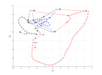
Figure 2: Robot trajectories. The triangles denote the orientation for $\alpha_{k}=\beta_{k}=1$.

\psfragscanon\psfrag{d1111111111}[Bc][B1][0.35][0]{$\mathfrak{H}^{1}(\bar{x}_{1},t)$}\psfrag{e1111111111}[Bc][B1][0.35][0]{$\mathfrak{H}^{2}(\bar{x}_{2},t)$}\psfrag{f1111111111}[Bc][B1][0.35][0]{$\mathfrak{H}^{3}(\bar{x}_{3},t)$}\includegraphics[width=170.71652pt]{barrier2}

Figure 3: Fixed-time convergent barrier functions evolution for $\alpha_{k}=\beta_{k}=0.4$.

V Conclusion

Based on a new notion of time-varying fixed-time convergent control barrier functions, we presented a feedback control strategy to find robust solutions for the performance of the multi-agent systems under conflicting local STL tasks. In particular, the lower bound of the introduced TFCBFs and the finite convergence time can be characterized in a user-specified way, independent of the initial conditions of the agents. Future works extend these results to more general collaborative tasks, including leader-follower topologies.

References

• [1] M. Kloetzer and C. Belta, “Automatic deployment of distributed teams of robots from temporal logic motion specifications,” IEEE Trans. Rob., vol. 26, no. 1, pp. 48–61, 2010.
• [2] O. Maler and D. Nickovic, “Monitoring temporal properties of continuous signals,” in Formal Techniques, Modelling and Analysis of Timed and Fault-Tolerant Systems.   Springer, 2004, pp. 152–166.
• [3] G. E. Fainekos and G. J. Pappas, “Robustness of temporal logic specifications for continuous-time signals,” Theor. Comput. Sci., vol. 410, no. 42, pp. 4262–4291, 2009.
• [4] A. D. Ames, X. Xu, J. W. Grizzle, and P. Tabuada, “Control barrier function based quadratic programs for safety critical systems,” IEEE Trans. Autom. Control, vol. 62, no. 8, pp. 3861–3876, 2017.
• [5] S. Kolathaya and A. D. Ames, “Input-to-state safety with control barrier functions,” IEEE Control Syst. Lett., vol. 3, no. 1, pp. 108–113, 2018.
• [6] X. Xu, P. Tabuada, J. W. Grizzle, and A. D. Ames, “Robustness of control barrier functions for safety critical control,” IFAC-PapersOnLine, vol. 48, no. 27, pp. 54–61, 2015.
• [7] P. Glotfelter, J. Cortés, and M. Egerstedt, “Nonsmooth barrier functions with applications to multi-robot systems,” IEEE Control Syst. Lett., vol. 1, no. 2, pp. 310–315, 2017.
• [8] W. Xiao and C. Belta, “Control barrier functions for systems with high relative degree,” in 58th Conf. Decision Control.   IEEE, 2019, pp. 474–479.
• [9] X. Xu, “Constrained control of input–output linearizable systems using control sharing barrier functions,” Automatica, vol. 87, pp. 195–201, 2018.
• [10] M. Z. Romdlony and B. Jayawardhana, “Uniting control lyapunov and control barrier functions,” in 53rd Conf. Decision Control.   IEEE, 2014, pp. 2293–2298.
• [11] K. Garg and D. Panagou, “Distributed robust control synthesis for safety and fixed-time stability in multi-agent systems,” arXiv preprint arXiv:2004.01054, 2020.
• [12] M. Black, K. Garg, and D. Panagou, “A quadratic program based control synthesis under spatiotemporal constraints and non-vanishing disturbances,” in 59th Conf. Decision Control.   IEEE, 2020, pp. 2726–2731.
• [13] L. Lindemann and D. V. Dimarogonas, “Control barrier functions for multi-agent systems under conflicting local signal temporal logic tasks,” IEEE Control Syst. Lett., vol. 3, no. 3, pp. 757–762, 2019.
• [14] ——, “Decentralized control barrier functions for coupled multi-agent systems under signal temporal logic tasks,” in 18th Euro. Control Conf.   IEEE, 2019, pp. 89–94.
• [15] A. Polyakov, “Nonlinear feedback design for fixed-time stabilization of linear control systems,” IEEE Trans. Autom. Control, vol. 57, no. 8, pp. 2106–2110, 2012.
• [16] Y. Liu, J. J. Zhu, R. L. Williams II, and J. Wu, “Omni-directional mobile robot controller based on trajectory linearization,” Rob. Auton. Syst., vol. 56, no. 5, pp. 461–479, 2008.
• [17] L. Lindemann and D. V. Dimarogonas, “Control barrier functions for signal temporal logic tasks,” IEEE Control Syst. Lett., vol. 3, no. 1, pp. 96–101, 2018.