We propose a new, flexible model for inference of the effect of a binary treatment on a continuous outcome observed over subsequent time periods. The model allows to seperate association due to endogeneity of treatment selection from additional longitudinal association of the outcomes and hence unbiased estimation of dynamic treatment effects. We investigate the performance of the proposed method on simulated data and employ it to reanalyse data on the longitudinal effects of a long maternity leave on mothers’ earnings after their return to the labour market.

1 Introduction

Identification and estimation of treatment effects is an important issue in many fields, e.g. to evaluate the effectiveness of social programs, government policies or medical interventions. As each subject is observed only either under control conditions or under treatment, the outcome difference which would allow straightforward estimation of treatment effects is not available for any particular subject. Additionally, for data from observational studies, endogeneity of treatment selection can cause unobserved confounding and bias of treatment effects estimates if not adequately accounted for.

Bayesian approaches to inference on treatment effects rely on specifying a joint model of treatment selection and the two potential outcomes, under control conditions and under treatment, of which only one is observed for each subject. To estimate the effect of a binary treatment on a continuous outcome observed over subsequent time periods two models, the switching regression model (Chib and Jacobi, 2007) and the shared factor model (Carneiro et al., 2003), have been suggested so far.

Both approaches rely on a binary regression model for selection into treatment and two multivariate regression models for the outcome sequences under control and under treatment, however they differ with respect to modeling the dependence across these regression models: Whereas Carneiro et al. (2003) model the association between treatment selection and both potential outcome sequences via shared latent factors, Chib and Jacobi (2007) specify only two marginal models for selection into treatment and one sequence of potential outcomes but leave the joint distribution of the two potential outcomes sequences unspecified.

Investigating both models in detail, Jacobi et al. (2016) show that both frameworks impose restrictions on the joint correlation structure of treatment selection and the two outcomes sequences that can result in biased treatment effects estimates if the assumptions on the correlation structure of the model used for data analysis are violated in the data generating process.

To increase flexibility in the dependence structure of treatment selection and potential outcomes we propose in the present paper a factor-augmented treatment effect model which extends the factor structure of the joint distribution to a bi-factor model. The bi-factor model was introduced in Holzinger and Swineford (1937) and recently gained popularity in item response analyses, see e.g. Reise (2012). Its basic assumption is that the covariance structure of multiple responses can be modelled by orthogonal factors where one common (or general) factor is shared by all responses and one or more further group (or specific) factors model the additional correlation among clusters of responses. This is attractive for jointly modelling of treatment selection and the two potential outcomes sequences as it allows to model association due to endogeneity of treatment selection as well as additional longitudinal association of the outcomes sequences: the general factor shared by the binary selection and both potential outcomes sequences accounts for unobserved confounding whereas outcome specific factors allow to model the additional longitudinal association that cannot be attributed to the unobserved confounders.

The paper is structured as follows. Section 2 discusses Bayesian treatment effects models for panel outcomes and reviews the switching regression and the shared factor model. Section 3 introduces the factor-augmented treatment effect model, discusses identification issues and describes posterior inference using MCMC methods. In Section 4, the flexibility of the factor-augmented treatment effect model is illustrated on simulated data. Section 5 provides a reanalysis of longitudinal effects of a long maternity leave on mothers’ earnings after their return to the labour market and Section 6 concludes.

2 Bayesian modelling of panel treatment effects

Assessing the effect of a treatment on an outcome of interest requires a comparison of this outcome under two conditions: with and without treatment ( control conditions). As typically each subject is observed only under either treatment or control conditions modelling of treatment effects relies on the potential outcomes framework (Rubin, 1981), which allows to define treatment effects based on models for the outcome under treatment as well as under control conditions. However, inference on treatment effects from observational data is demanding as in addition to the fundamental problem that only one potential outcome is observed for each subject, treatment is not randomized, but self selected and hence might be associated to the outcome.

To take endogeneity of treatment selection into account, Bayesian approaches to modelling treatment effects rely on specifying a joint model for treatment selection and the potential outcomes, often in the spirit of Roy’s switching regression model (Roy, 1951; Lee, 1978). For longitudinally observed outcomes, two approaches have been suggested sofar: Chib and Jacobi (2007) specify two models for selection into treatment and one potential outcomes sequence respectively, whereas Carneiro et al. (2003) specify a joint model for selection into treatment and the two potential outcomes models. Jacobi et al. (2016) use both approaches to analyse the effects of a longer maternity leave on the earnings of mothers.

While the switching regression model as well as the shared factor model rely on a probit model for treatment selection and two multivariate normal regression models for the potential outcomes sequences, they differ with respect to modelling their joint distributions. To discuss these differences in more detail, we introduce the marginal models for latent utilities and the potential outcomes sequences in Section 2.1 and describe modelling of the dependence structure in both approaches in Section 2.2.

2.1 Marginal models for treatment selection and outcomes sequences

Let $x_{i},i=1,\dots,n$ denote the treatment status of each subject $i$ for $i=1,\dots,n$. Treatment selection depends on covariates (selection on observables) via a probit model for $x_{i}$, which can be specified in terms of a latent Gaussian random variable $x_{i}^{*}$ as

$$x_{i}^{*} =\mathbf{v}_{i}\boldsymbol{\alpha}+\varepsilon_{xi},\qquad \varepsilon_{xi}\sim\mathcal{N}\left(0,\sigma^{2}_{x}\right),$$ (1)

$$x_{i} =I_{\{x_{i}^{*}>0\}},$$ (2)

where $\mathbf{v}_{i}$ denotes the row vector of covariates and $\boldsymbol{\alpha}$ their effect on treatment selection. Note that different from the usual specification of a probit model, (1) leaves the variance of the error term unspecified, whereas usually the error variance of the latent utility is fixed to 1, $\sigma^{2}_{x}=1$, as regression effects $\boldsymbol{\alpha}$ are only identified up to a scale factor. However, in factor models where the error term $\varepsilon_{xi}$ is modelled by a latent factor plus an idiosyncratic error it is more convenient to fix the variance of the idiosyncratic error to one.

The selection model given in equations (1) and (2) is combined with a model for the potential outcomes for subject $i$ at time points $t=1,\dots,T$ which we denote by $y_{0,it}$ and $y_{1,it}$ for the outcome under control conditions and treatment, respectively. The potential outcomes are modelled as

$$y_{0,it} =\eta_{0,it}(\mathbf{w}_{it})+\varepsilon_{0,it},\qquad \varepsilon_{0,it}\sim\mathcal{N}\left(0,\sigma^{2}_{0t}\right),$$ (3)

$$y_{1,it} =\eta_{1,it}(\mathbf{w}_{it})+\varepsilon_{1,it},\qquad \varepsilon_{1,it}\sim\mathcal{N}\left(0,\sigma^{2}_{1t}\right),$$ (4)

with structural means $\eta_{j,it}(\mathbf{w}_{it})$ for $j=0,1$ depending a row vector of covariates $\mathbf{w}_{it}$:

$$\eta_{0,it}(\mathbf{w}_{it}) =\mu_{t}+\mathbf{w}_{it}\boldsymbol{\gamma}$$ (5)

$$\eta_{1,it}(\mathbf{w}_{it}) =(\mu_{t}+\kappa_{t})+\mathbf{w}_{it}(\boldsymbol{\gamma}+\boldsymbol{\theta}).$$ (6)

Here, $\mu_{t}$ and $\mu_{t}+\kappa_{t}$ are the intercepts and $\boldsymbol{\gamma}$ and $\boldsymbol{\gamma}+\boldsymbol{\theta}$ the vectors of covariate effects under, respectively, control conditions and under treatment. With this specification, the average treatment effect of a subject with covariate values $\mathbf{w}_{it}$ in panel period $t$ results as

$$E({y}_{1,it}-y_{0,it}|\mathbf{w}_{it})=\kappa_{t}+\mathbf{w}_{it}\boldsymbol{\theta}.$$

However, the observed outcome $y_{it}|(x_{i}=j)$ conditional on knowing $x_{i}=j$ is equal to $y_{0,it}$, if $x_{i}=0$, and equal to $y_{1,it}$, if $x_{i}=1$. Or, in terms of the latent utility $x_{i}^{*}$ introduced in equation (1):

$$y_{it}|x_{i}^{*}=\begin{cases}y_{0,it},\quad&\text{for }x_{i}^{*}<0,\\ y_{1,it},\quad&\text{for }x_{i}^{*}\geq 0.\end{cases}$$

In randomized studies, treatment selection $x_{i}$ is independent from the observed outcome. Hence, $y_{it}|(x_{i}=j)$ has the same distribution as $y_{j,it}$, which allows straightforward estimation of the average treatment effects from the observed outcomes. This is, however, not the case in observational studies where subjects choose treatment based on their expectations on the outcomes and therefore explicit modelling of the association between treatment selection and observed outcome is necessary. We return to this issue in Section 2.2.

In the following, we will denote the vectors of potential outcomes by $\mathbf{y}_{ji}=({y}_{j,i1},\dots,{y}_{j,iT})$ for $j=0,1$ and by $\mathbf{y}_{i}|(x_{i}=j)=\big{(}{y}_{i1}|(x_{i}=j),\dots,{y}_{iT}|(x_{i}=j)\big{)}$ the vector of observed outcomes for subject $i$.

2.2 Modelling the dependence structure

As noted above, endogeneity of treatment selection (selection on unobservables) can be taken into account by allowing for correlation of treatment selection and the potential outcomes. This approach is followed both by the switching regression as well as the shared factor model. However, the impossibility to observe both outcomes $\mathbf{y}_{0i}$ and $\mathbf{y}_{1i}$ for the same subject $i$ makes it impossible to observe the joint distribution of the errors $(\boldsymbol{\varepsilon}_{0i},\boldsymbol{\varepsilon}_{1i})^{\prime}$ and the two models differ with respect to specifying the error distribution.

In the switching regression model, the joint distribution of $(\boldsymbol{\varepsilon}_{0i},\boldsymbol{\varepsilon}_{1i})$ is left unspecified and only the two joint $(T+1)$-variate distributions of the latent utility error $\varepsilon_{xi}$ and the errors $\boldsymbol{\varepsilon}_{ji}=(\varepsilon_{j,i1},\dots,\varepsilon_{j,iT})^{\prime}$ in each outcome equation, i.e. the marginal distributions of $(\varepsilon_{xi},\boldsymbol{\varepsilon}_{0i})$ and $(\varepsilon_{xi},\boldsymbol{\varepsilon}_{1i})$, are specified as multivariate normal distributions.

In contrast, in the shared factor model the joint $(2T+1)$-dimensional distribution of all error terms ($\varepsilon_{xi},\boldsymbol{\varepsilon}_{0i},\boldsymbol{\varepsilon}_{1i})$ is modelled in terms of latent factors and independent idiosyncratic errors. Carneiro et al. (2003) specify a multi-factor model and exploit additional measurements from psychological tests to identify factors and factor loadings. Such additional measurements are not available in the analysis of Jacobi et al. (2016) who therefore use a simpler factor structure with only one subject specific random factor that accounts for within subject dependence as well as endogeneity. They specify the error terms as

$$\varepsilon_{xi} =\lambda_{x}f_{i}+\epsilon_{xi},\qquad \epsilon_{xi}\sim\mathcal{N}\left(0,1\right),$$ (7)

$$\boldsymbol{\varepsilon}_{ji} =\boldsymbol{\lambda}_{j}f_{i}+\boldsymbol{\epsilon}_{ji},\qquad \boldsymbol{\epsilon}_{ji}\sim\mathcal{N}\left(\mathbf{0},\mathbf{S}_{j}=\operatorname{diag}(\sigma^{2}_{j1},\dots,\sigma^{2}_{jT})\right),\quad j=0,1,$$ (8)

where $f_{i}\sim\mathcal{N}\left(0,1\right)$ is an unobserved subject specific factor, $\lambda_{x}$ is its loading on the latent utility and $\boldsymbol{\lambda}_{j}=(\lambda_{j1},\dots,\lambda_{jT})^{\prime}$, $j=0,1$ denote the vectors of factor loadings for the potential outcomes. $\epsilon_{xi}$ and $\boldsymbol{\epsilon}_{ji}$, $j=0,1$ are the idiosyncratic errors of the latent utility and the potential outcome vectors, respectively. Both, factor loadings $\lambda_{jt}$ as well as the variances $\sigma^{2}_{jt}$ of the idiosyncratic errors are allowed to vary over time. The joint covariance matrix of the vector $\boldsymbol{\varepsilon}_{i}=(\varepsilon_{xi},\boldsymbol{\varepsilon}_{0i}^{\prime},\boldsymbol{\varepsilon}_{1i}^{\prime})^{\prime}$ is then given as

$$\operatorname{Cov}(\boldsymbol{\varepsilon}_{i})=\boldsymbol{\Sigma}=\begin{pmatrix}\sigma_{x}^{2}&\boldsymbol{\sigma}_{x0}^{\prime}&\boldsymbol{\sigma}_{x1}^{\prime}\\ \boldsymbol{\sigma}_{x0}&\boldsymbol{\Sigma}_{0}&\boldsymbol{\Sigma}_{01}\\ \boldsymbol{\sigma}_{x1}&\boldsymbol{\Sigma}_{01}&\boldsymbol{\Sigma}_{1}\end{pmatrix}=\begin{pmatrix}1+\lambda_{x}^{2}&\lambda_{x}\boldsymbol{\lambda}_{0}^{\prime}&\lambda_{x}\boldsymbol{\lambda}_{1}^{\prime}\\ \lambda_{x}\boldsymbol{\lambda}_{0}&\boldsymbol{\lambda}_{0}\boldsymbol{\lambda}_{0}^{\prime}+\mathbf{S}_{0}&\boldsymbol{\lambda}_{0}\boldsymbol{\lambda}_{1}^{\prime}\\ \lambda_{x}\boldsymbol{\lambda}_{1}&\boldsymbol{\lambda}_{0}\boldsymbol{\lambda}_{1}^{\prime}&\boldsymbol{\lambda}_{1}\boldsymbol{\lambda}_{1}^{\prime}+\mathbf{S}_{1}\end{pmatrix}.$$

Hence, for fixed covariates, $\boldsymbol{\sigma}_{xj}=\operatorname{Cov}(x_{i}^{*},\mathbf{y}_{ji})$ denotes the vector of covariances between the latent utility $x_{i}^{*}$ and the potential outcome vector $\mathbf{y}_{ji}$, and $\boldsymbol{\Sigma}_{j}=\operatorname{Cov}(\mathbf{y}_{ji})$ is the covariance matrix of the potential outcome vector $\mathbf{y}_{ji}$ for $j=0,1$. Most importantly, the covariance matrix of the two potential outcome vectors $\mathbf{y}_{0i}$ and $\mathbf{y}_{1i}$, $\boldsymbol{\Sigma}_{01}=\operatorname{Cov}(\mathbf{y}_{0i},\mathbf{y}_{1i})$, is modelled explicitly. The assumption that the latent factor $f_{i}$ is shared by the latent utility and all potential outcomes implies that the vectors of time-varying factor loadings $\boldsymbol{\lambda}_{j}$, $j=0,1$ determine not only $\boldsymbol{\Sigma}_{j}$ (and thus the correlation within each potential outcome vector) and $\boldsymbol{\sigma}_{xj}=\lambda_{x}\boldsymbol{\lambda}_{j}$ (and thus the correlation between latent utility and each potential outcome vector), but also $\boldsymbol{\Sigma}_{01}$ and thus the correlation between the potential outcome vectors. Note, however, that this assumption is not testable from empirical data where only one potential outcome is observed for each subject.

In contrast, in the switching regression model a latent factor is assumed to model only the correlations within one potential outcomes vector

$$\boldsymbol{\varepsilon}_{ji}=\boldsymbol{\lambda}_{j}f_{ji}+\boldsymbol{\epsilon}_{ji},\qquad\boldsymbol{\epsilon}_{ji}\sim\mathcal{N}\left(\mathbf{0},\mathbf{S}_{j}\right),\quad j=0,1,$$

where (as in the shared factor model) $\mathbf{S}_{j}=\operatorname{diag}(\sigma^{2}_{j1},\dots,\sigma^{2}_{jT})$ is the variance matrix of the idiosyncratic errors. The latent factors $f_{0i}$ and $f_{1i}$ are assumed to have standard normal marginal distributions, $f_{ji}\sim\mathcal{N}\left(0,1\right)$, but no assumption is made on their joint distribution. While the error term of the latent utility, $\varepsilon_{xi}=\epsilon_{xi}$, is independent of the factors, it is allowed to be correlated with the idiosyncratic errors $\boldsymbol{\epsilon}_{ji}$ of each potential outcome equation, to capture selection on unobservables. Hence, the joint $(T+1)$-variate distributions of the idiosyncratic errors $(\epsilon_{xi},\boldsymbol{\epsilon}_{ji}^{\prime})$ are given as

$$(\epsilon_{xi},\boldsymbol{\epsilon}_{ji}^{\prime})^{\prime}\sim\mathcal{N}\left(\mathbf{0},\begin{pmatrix}1&\boldsymbol{\omega}_{j}^{\prime}\\ \boldsymbol{\omega}_{j}&\mathbf{S}_{j}\end{pmatrix}\right),\quad j=0,1,$$ (9)

where the vector $\boldsymbol{\omega}_{j}$ of covariances between the latent utility and potential outcome vector $\mathbf{y}_{ji}$ is completely unstructured.

Both models have drawbacks. The shared factor model relies on the untestable assumption that the latent factor is shared by the latent utility and both potential outcomes. Hence, as the factor loadings determine all correlations in the multivariate normal distribution of the errors $\boldsymbol{\varepsilon}_{ji}$, this correlation structure is not fully flexible. On the other hand, in the switching regression model no joint model for the error terms is specified and the variance of the outcome difference is not available. Additionally, the assumption that each latent factor affects only the corresponding potential outcomes vector, but not the latent utility, implies that, conditional on the latent utility error $\epsilon_{xi}$, the idiosyncratic errors $\boldsymbol{\epsilon}_{ji}$ in the potential outcome model are negatively correlated over time, since equation (9) implies following covariance matrix of $\boldsymbol{\epsilon}_{ji}$ given $\epsilon_{xi}$:

$$\operatorname{Cov}(\boldsymbol{\epsilon}_{ji}|\epsilon_{xi})=\mathbf{S}_{j}-\boldsymbol{\omega}_{j}\boldsymbol{\omega}_{j}^{\prime}.$$

None of the models encompasses the other, but the positive semi-definiteness of the specified covariance matrices can result in restrictions on their elements in one model which cannot be recovered under the other. Thus, as shown in a simulation study in Jacobi et al. (2016), treatment effects can be biased, when data generated under the shared factor model are analysed using the switching regression model and vice versa.

3 A factor-augmented treatment effects model

In this section we propose a factor-augmented model for modelling the joint distribution of the latent utility and the two potential outcomes sequences to allow for a flexible dependence structure where the correlation within an outcomes sequence is disentangled into correlation due to confounding and additional longitudinal correlation. We introduce the model in Section 3.1 and discuss identification issues in Section 3.2. Section 3.3 describes specification of the prior distributions and Section 3.4 outlines posterior inference.

3.1 Model specification

We consider the model specified in Section 2.1, with a probit model for treatment selection given in equations (1) and (2) and the model for the potential outcome sequences $\mathbf{y}_{0i}$ and $\mathbf{y}_{1i}$ given as

$$\mathbf{y}_{0i} =\boldsymbol{\mu}+\mathbf{W}_{i}\boldsymbol{\theta}+\boldsymbol{\varepsilon}_{0i},$$ (10)

$$\mathbf{y}_{1i} =\boldsymbol{\mu}+\boldsymbol{\kappa}+\mathbf{W}_{i}(\boldsymbol{\theta}+\boldsymbol{\gamma})+\boldsymbol{\varepsilon}_{1i},$$ (11)

where $\mathbf{W}_{i}$ is the corresponding matrix of covariate values with rows $\mathbf{w}_{i1},\ldots,\mathbf{w}_{iT}$ and $\boldsymbol{\mu}$ and $\boldsymbol{\kappa}$ are the vectors $\boldsymbol{\mu}=(\mu_{1},\dots,\mu_{T})$ and $\boldsymbol{\kappa}=(\kappa_{1},\dots,\kappa_{T})$.

To achieve more flexibility in modelling the association of treatment selection and the potential outcomes sequences, we assume that all dependencies in the error vector $\boldsymbol{\varepsilon}_{i}=(\varepsilon_{xi},\boldsymbol{\varepsilon}_{0i}^{\prime},\boldsymbol{\varepsilon}_{1i}^{\prime})^{\prime}$ are captured by three subject specific latent factors: one common factor $f_{ci}$ which is shared by the error terms of the latent utility $x^{*}_{i}$ and both potential outcome vectors $\mathbf{y}_{0i}$ and $\mathbf{y}_{1i}$ and two specific factors $f_{0i}$ and $f_{1i}$ which affect only the error vectors of the potential outcome $\boldsymbol{\varepsilon}_{0i}$ and $\boldsymbol{\varepsilon}_{1i}$ respectively.

The common factor thus accounts for unobserved confounding whereas the two outcome specific factors $f_{0i}$ and $f_{1i}$ capture the additional longitudinal association in the outcome vectors that cannot be attributed to unobserved confounders. The joint model for the error terms is thus specified as

$$\varepsilon_{xi} =\lambda_{x}f_{ci}+\epsilon_{xi},\qquad \epsilon_{xi}\sim\mathcal{N}(0,1),$$ (12)

$$\boldsymbol{\varepsilon}_{0i} =\boldsymbol{\lambda}_{0}f_{ci}+\boldsymbol{\boldsymbol{\zeta}}_{0}f_{0i}+\boldsymbol{\epsilon}_{0i},\qquad \epsilon_{0,it}\sim\mathcal{N}(0,\sigma^{2}_{0t}),$$ (13)

$$\boldsymbol{\varepsilon}_{1i} =\boldsymbol{\lambda}_{1}f_{ci}+\boldsymbol{\boldsymbol{\zeta}}_{1}f_{1i}+\boldsymbol{\epsilon}_{1i},\qquad \epsilon_{1,it}\sim\mathcal{N}(0,\sigma^{2}_{1t}),$$ (14)

where the factors $f_{ci}$, $f_{0i}$ and $f_{1i}$ are assumed to be independent standard normals. Hence, the factor loadings $\lambda_{x}$, $\boldsymbol{\lambda}_{j}$ and $\boldsymbol{\zeta}_{j}$, $j=0,1$ determine the joint variance-covariance matrix of all error terms.

Assumptions on how factors are related to outcomes simplify the structure of the factor loadings matrix. First, treatment selection and both outcome panels depend on the common factor $f_{ci}$ with loadings $\lambda_{x}$ in the latent utility and $\boldsymbol{\lambda}_{j}$, $j=1,2$ for the two potential outcome. Second, the potential outcomes vector $\mathbf{y}_{ji}$ depends only on one specific factor $f_{ji}$ with loadings $\boldsymbol{\zeta}_{j}$.

In matrix form the factor model for the errors is given as

$$\boldsymbol{\varepsilon}_{i}=\boldsymbol{\Lambda}\mathbf{f}_{i}+\boldsymbol{\epsilon}_{i},\qquad\boldsymbol{\Lambda}=\begin{pmatrix}\lambda_{x}&0&0\\ \boldsymbol{\lambda}_{0}&\boldsymbol{\zeta}_{0}&\mathbf{0}_{T}\\ \boldsymbol{\lambda}_{1}&\mathbf{0}_{T}&\boldsymbol{\zeta}_{1}\end{pmatrix},$$ (15)

where $\mathbf{f}_{i}=(f_{ci},f_{0i},f_{1i})^{\prime}$ is the vector of factors for subject $i$ and $\boldsymbol{\epsilon}_{i}=(\epsilon_{xi},\boldsymbol{\epsilon}_{0i}^{\prime},\boldsymbol{\epsilon}_{1i}^{\prime})^{\prime}$ is the vector of idiosyncratic errors. Hence, the joint $(2T+1)$-variate distribution of $\boldsymbol{\varepsilon}_{i}$ is multivariate normal, $\boldsymbol{\varepsilon}_{i}\sim\mathcal{N}\left(\mathbf{0},\boldsymbol{\Sigma}\right),$ with variance covariance matrix given as

$$\boldsymbol{\Sigma}=\begin{pmatrix}\sigma_{x}^{2}&\boldsymbol{\sigma}_{x0}^{\prime}&\boldsymbol{\sigma}_{x1}^{\prime}\\ \boldsymbol{\sigma}_{x0}&\boldsymbol{\Sigma}_{0}&\boldsymbol{\Sigma}_{01}\\ \boldsymbol{\sigma}_{x1}&\boldsymbol{\Sigma}_{01}&\boldsymbol{\Sigma}_{1}\end{pmatrix}=\begin{pmatrix}1+\lambda_{x}^{2}&\lambda_{x}\boldsymbol{\lambda}_{0}^{\prime}&\lambda_{x}\boldsymbol{\lambda}_{1}^{\prime}\\ \lambda_{x}\boldsymbol{\lambda}_{0}&\boldsymbol{\lambda}_{0}\boldsymbol{\lambda}_{0}^{\prime}+\boldsymbol{\zeta}_{0}\boldsymbol{\zeta}_{0}^{\prime}+\mathbf{S}_{0}&\boldsymbol{\lambda}_{0}\boldsymbol{\lambda}_{1}^{\prime}+\boldsymbol{\zeta}_{0}\boldsymbol{\zeta}_{1}^{\prime}\\ \lambda_{x}\boldsymbol{\lambda}_{1}&\boldsymbol{\lambda}_{0}\boldsymbol{\lambda}_{1}^{\prime}+\boldsymbol{\zeta}_{0}\boldsymbol{\zeta}_{1}^{\prime}&\boldsymbol{\lambda}_{1}\boldsymbol{\lambda}_{1}^{\prime}+\boldsymbol{\zeta}_{1}\boldsymbol{\zeta}_{1}^{\prime}+\mathbf{S}_{1}\end{pmatrix}.$$

Though an extension to multiple independent outcome specific factors $\mathbf{f}_{ji}$ is straightforward conceptually, to achieve identification of the factor loadings from the observed data the dimension of outcome specific factors is restricted by the number of available panel observations $T$. We will return to this issue in Section 3.2 but note here that in contrast to Carneiro et al. (2003) we do not assume that additional measurements are available from which the latent factors can be identified.

Already the simple factor-augmented model specified above avoids drawbacks of both the shared factor and the switching regression model. As correlation across panel outcomes is not attributed solely to the common factor, it is more flexible than the shared factor model which is recovered as that special case where $\boldsymbol{\zeta}_{1}=\boldsymbol{\zeta}_{2}=\mathbf{0}$. Without any assumption on the joint distribution of the specific factors $f_{0i}$ and $f_{1i}$ the model is a switching regression model with the advantage that conditional on the latent factors the errors of latent utility and each potential outcome are independent.

3.2 Identification

An important issue in factor models is their identification, which according to Anderson and Rubin (1956) is a two-step procedure where the first step is identification of the variance contribution attributable to the latent factors, i.e. $\boldsymbol{\Lambda}\boldsymbol{\Lambda}^{\prime}$ and the second step is identification of $\boldsymbol{\Lambda}$, i.e. solving the rotational identification problem.

The data structure in the factor augmented treatment model proposed above, however, differs considerably from the standard factor model which assumes multivariate normal observations: only the binary treatment variable $x_{i}$ and the observed outcome sequence, which is a truncated version of one of the two potential outcomes sequences are observed for each subject. However, due to the general triangular structure of the factor loadings matrix rotational identification is not an issue for the bi-factor model, see Frühwirth-Schnatter and Lopes (2018).

In the probit model, identification of regression effects is feasible only up to the standard error $\sigma_{x}$ of the latent utility and hence only the standardized effects

$$\tilde{\boldsymbol{\alpha}}=\frac{\boldsymbol{\alpha}}{\sigma_{x}}=\frac{\boldsymbol{\alpha}}{\sqrt{1+\lambda^{2}_{x}}}$$

in model (1) are identified. Fixing $\sigma_{x}=1$ would in principle be possible, however require to restrict the range of the factor loading $\lambda_{x}$ to $(-1,1)$.

The observed data never provide information on the association between the two potential outcome vectors $\mathbf{y}_{0i}$ and $\mathbf{y}_{1i}$. Due to endogeneity of treatment selection the distribution of the observed outcome sequence $\mathbf{y}_{i}$ is not the marginal distribution of $\mathbf{y}_{ji}$, but the conditional distribution truncated by the respective range of the latent utility. It is given as

$$p(\mathbf{y}_{ji}|x_{i}=j)=\begin{cases}\frac{1}{1-\Phi(\tilde{\mu}_{x,i})}\int_{-\infty}^{0}p(\mathbf{y}_{0i},x_{i}^{*})dx_{i}^{*},&\quad j=0,\\ \frac{1}{\Phi(\tilde{\mu}_{x,i})}\int_{0}^{\infty}p(\mathbf{y}_{1i},x_{i}^{*})dx_{i}^{*},&\quad j=1,\end{cases}$$

where $\tilde{\mu}_{x,i}=\mathbf{v}_{i}\tilde{\boldsymbol{\alpha}}$ is the mean of the standardized latent utility $x_{i}^{*}/\sigma_{x}$.

Identification of all parameters that are not identified from the probit model, i.e. the regression effects in the potential outcomes models, the factor loadings and the variances of the idiosyncratic errors has to be accomplished from these two conditional distributions. We will discuss necessary conditions for identification of the model parameters from the first and second moments of these two conditional distributions.

The expectation of the observed outcomes sequence $\mathbf{y}_{i}|x_{i}=j$ is given as:

$$\operatorname{E}(\mathbf{y}_{i}|x_{i}=0) =\operatorname{E}(\mathbf{y}_{0i}|x_{i}=0)=\boldsymbol{\mu}+\mathbf{W}_{i}\boldsymbol{\gamma}-\frac{\boldsymbol{\sigma}_{0x}}{\sigma_{x}}\frac{\phi(\mathbf{v}_{i}\tilde{\boldsymbol{\alpha}})}{1-\Phi(\mathbf{v}_{i}\tilde{\boldsymbol{\alpha}})},$$

$$\operatorname{E}(\mathbf{y}_{i}|x_{i}=1) =\operatorname{E}(\mathbf{y}_{1i}|x_{i}=1)=\boldsymbol{\mu}+\boldsymbol{\kappa}+\mathbf{W}_{i}(\boldsymbol{\gamma}+\boldsymbol{\theta})+\frac{\boldsymbol{\sigma}_{1x}}{\sigma_{x}}\frac{\phi(\mathbf{v}_{i}\tilde{\boldsymbol{\alpha}})}{\Phi(\mathbf{v}_{i}\tilde{\boldsymbol{\alpha}})},$$

see Appendix A for details. As the quantities $c_{i0}(\mathbf{v}_{i}\tilde{\boldsymbol{\alpha}})=-\frac{\phi(\mathbf{v}_{i}\tilde{\boldsymbol{\alpha}})}{1-\Phi(\mathbf{v}_{i}\tilde{\boldsymbol{\alpha}})}$ and $c_{i1}(\mathbf{v}_{i}\tilde{\boldsymbol{\alpha}})=\frac{\phi(\mathbf{v}_{i}\tilde{\boldsymbol{\alpha}})}{\Phi(\mathbf{v}_{i}\tilde{\boldsymbol{\alpha}})}$ are identified from the probit model, identification of the parameters $\boldsymbol{\mu},\boldsymbol{\kappa},\boldsymbol{\gamma},\boldsymbol{\theta}$ and $\tilde{\boldsymbol{\sigma}}_{jx}=\frac{\boldsymbol{\sigma}_{jx}}{\sigma_{x}}$, for $j=0,1$ is feasible from these equations, if the design matrix in the corresponding regression model is of full rank. $\frac{\boldsymbol{\sigma}_{0x}}{\sigma_{x}}$ and $\frac{\boldsymbol{\sigma}_{0x}}{\sigma_{x}}$ yield $2T$ equations for the $2T+1$ factor loadings $\boldsymbol{\lambda}$ of the common factor, leaving at least one of these factor loadings unidentfied. The conditional covariance matrices $\operatorname{V}(\mathbf{y}_{i}|x_{i}=0)$ and $\operatorname{V}(\mathbf{y}_{i}|x_{i}=1)$, given as

$$\operatorname{V}(\mathbf{y}_{i}|x_{i}=0) =\boldsymbol{\Sigma}_{0}-c_{i0}(\mathbf{v}_{i}\tilde{\boldsymbol{\alpha}})\Big{(}\mathbf{v}_{i}\tilde{\boldsymbol{\alpha}}+c_{i0}(\mathbf{v}_{i}\tilde{\boldsymbol{\alpha}})\Big{)}{\tilde{\boldsymbol{\sigma}}_{x0}}^{\prime}{\tilde{\boldsymbol{\sigma}}_{x0}},$$

$$\operatorname{V}(\mathbf{y}_{i}|x_{i}=1) =\boldsymbol{\Sigma}_{1}-c_{i1}(\mathbf{v}_{i}\tilde{\boldsymbol{\alpha}})\Big{(}\mathbf{v}_{i}\tilde{\boldsymbol{\alpha}}+c_{i1}(\mathbf{v}_{i}\tilde{\boldsymbol{\alpha}})\Big{)}{\tilde{\boldsymbol{\sigma}}_{x1}}^{\prime}{\tilde{\boldsymbol{\sigma}}_{x1}},$$

have $\frac{T(T+1)}{2}$ free elements each, from which one element of $\boldsymbol{\lambda}$, the factor loadings $\boldsymbol{\zeta}_{0}$ and $\boldsymbol{\zeta}_{1}$ and the variances $\boldsymbol{\sigma}^{2}_{0}$ and $\boldsymbol{\sigma}^{2}_{1}$ have to be identified. Thus, a necessary condition for identification is that

$$T(T+1)\geq 4T+1,$$

and hence that the observed panel outcomes are at least of length $T\geq 4$. Generally, as a necessary condition for identification of the parameters in a model with $r>1$ outcome specific factors is that

$$T(T+1)\geq 2(r+1)T+1,$$

the outcome panels have to be at least of length $T=6$ and $T=8$ to identify the loadings of $r=2$ or $r=3$ outcome specific factors, respectively. Identification of the elements of $\boldsymbol{\lambda}_{0}$, $\boldsymbol{\lambda}_{1}$, $\boldsymbol{\zeta}_{0}$ and $\boldsymbol{\zeta}_{1}$, however, requires also that enough factor loadings are different from $0$, see Anderson and Rubin (1956); Conti et al. (2014); Frühwirth-Schnatter and Lopes (2018).

3.3 Prior distributions

To complete the Bayesian model specification, prior distributions are assigned to all model parameters. We write the model for the observed outcome vector of subject $i$ compactly as

$$y_{it}|(x_{i}=j)=\mathbf{w}_{j,it}\boldsymbol{\beta}+\varepsilon_{j,it},$$

where $\boldsymbol{\beta}=(\boldsymbol{\mu},\boldsymbol{\kappa},\boldsymbol{\gamma},\boldsymbol{\theta})$ comprises all regression parameters in both outcome models and $\mathbf{w}_{j,it}$ denotes the corresponding covariates at panel time $t$. Thus the factor-augmented (FA) treatment model is given as

$$x_{i}^{*} =\mathbf{v}_{i}\boldsymbol{\alpha}+\lambda_{x}f_{i}+\epsilon_{xi}, \epsilon_{xi}\sim \mathcal{N}\left(0,1\right),$$

$$\mathbf{y}_{i}|(x_{i}=j) =\mathbf{W}_{ji}\boldsymbol{\beta}+\boldsymbol{\lambda}_{j}f_{ci}+\boldsymbol{\zeta}_{j}f_{ji}+\boldsymbol{\epsilon}_{ji}, \boldsymbol{\epsilon}_{ji}\sim \mathcal{N}_{T}\left(\mathbf{0},\mathbf{S}_{j}\right),$$

where the $t$th row of $\mathbf{W}_{ji}$ is equal to $\mathbf{w}_{j,it}$.

We assume that the regression parameters $\boldsymbol{\alpha}$, $\boldsymbol{\beta}$, the factor loadings $\lambda_{x},\boldsymbol{\lambda}_{0},\boldsymbol{\lambda}_{1}$, $\boldsymbol{\zeta}_{0}$, $\boldsymbol{\zeta}_{1}$ and the variances of the idiosyncratic errors $\mathbf{S}_{0},\mathbf{S}_{1}$ are independent apriori.

Following Jacobi et al. (2016), we perform variable selection in the selection as well as the outcome model to avoid overspecification. We assume prior independence of all coefficients in $\boldsymbol{\alpha}$ and $\boldsymbol{\beta}$ and specify normal priors $\mathcal{N}\left(0,V_{\alpha}\right)$ and $\mathcal{N}\left(0,V_{\beta}\right)$, respectively, for the coefficients in $\boldsymbol{\alpha}$ and $\boldsymbol{\beta}$ not subject to selection. In our application, these are the intercept in the selection equation and $\mu_{1}$ in the outcome equation and we use $V_{\alpha}=5$ and $V_{\beta}=10^{4}$.

For all coefficients in $\boldsymbol{\alpha}$ and $\boldsymbol{\beta}$ subject to selection, we employ spike and slab priors with a Dirac spike at 0. A spike and slab prior is a mixture of a component concentrated at zero, the spike, and a comparably flat component, the slab. A Dirac spike and slab prior has a Dirac spike at zero. For each coefficient in $\boldsymbol{\beta}$ subject to selection, $\beta_{\ell}$, this prior is specified hierarchically as

$$p(\beta_{\ell})=\delta^{\beta}_{\ell}p(\beta_{\ell}|\delta^{\beta}_{\ell}=1)+(1-\delta^{\beta}_{\ell})I_{0}(\beta_{\ell}),$$

depending on a binary variable $\delta^{\beta}_{\ell}$ with prior inclusion probability $p(\delta^{\beta}_{\ell}=1)=\pi_{\beta}$ and $\pi_{\beta}\sim\mathcal{B}\left(a,b\right)$. A similar prior is introduced for each coefficient in $\boldsymbol{\alpha}$ subject to selection, $\alpha_{\ell}$, involving a binary indicator $\delta^{\alpha}_{\ell}$ with prior inclusion probability $p(\delta^{\alpha}_{\ell}=1)=\pi_{\alpha}$ and $\pi_{\alpha}\sim\mathcal{B}\left(a,b\right)$. In our application, we use normal slabs with zero mean and variance 5 and uniform priors $\mathcal{B}\left(1,1\right)$ on the inclusion probabilities $\pi_{\alpha}$ and $\pi_{\beta}$.

All indicator variables are subsumed in the vectors $\boldsymbol{\delta}^{\alpha}$ and $\boldsymbol{\delta}^{\beta}$, respectively, and estimated along with the model parameters during MCMC estimation (see Section 3.4). Note that estimation of indicators $\delta^{\beta}_{\ell}$ corresponding to coefficients in the parameter $\boldsymbol{\gamma}$ identifies relevant predictors for the outcome equation under control. Most importantly, estimation of indicators $\delta^{\beta}_{\ell}$ corresponding to coefficients in $\boldsymbol{\theta}$ leads to the identification of heterogeneous treatment effects.

Finally, we assume that all elements in the factor loading vectors, $\lambda_{x},\boldsymbol{\lambda}_{0},\boldsymbol{\lambda}_{1}$, $\boldsymbol{\zeta}_{0}$, $\boldsymbol{\zeta}_{1}$, a priori are independent standard normal $\mathcal{N}\left(0,1\right)$. Also the variances $\sigma^{2}_{jt}$ of the idiosyncratic errors are assumed to be independent and assigned a $\mathcal{G}^{-1}\left(s_{0j},S_{0j}\right)$ prior. We use $s_{0j}=S_{0j}=2.5$ in our application.

3.4 Posterior inference

Posterior inference can be accomplished by Markov chain Monte Carlo (MCMC) methods, extending Jacobi et al. (2016).

As the idiosyncrativ errors $\epsilon_{xi},\boldsymbol{\epsilon}_{0i},\boldsymbol{\epsilon}_{1i}$ are independent, the augmented likelihood including the unobserved latent utilities is given as

$$p(\mathbf{x},\mathbf{x}^{*},\mathbf{y}|\boldsymbol{\Theta},\mathbf{f})=\prod_{i=1}^{n}p(x_{i},x_{i}^{*}|\boldsymbol{\alpha},\lambda_{x},f_{ci}) \cdot\prod_{i:x_{i}=0}p(\mathbf{y}_{0i}|\boldsymbol{\beta},\mathbf{S}_{0},\boldsymbol{\lambda}_{0},\boldsymbol{\zeta}_{0},f_{ci},f_{0i})\cdot$$

$$\cdot\prod_{i:x_{i}=1}p(\mathbf{y}_{1i}|\boldsymbol{\beta},\mathbf{S}_{1},\boldsymbol{\lambda}_{1},\boldsymbol{\zeta}_{1},f_{ci},f_{1i}),$$

Here $\mathbf{f}=(\mathbf{f}_{c},\mathbf{f}_{0},\mathbf{f}_{1})$, where $\mathbf{f}_{c}$, $\mathbf{f}_{0}$ and $\mathbf{f}_{1}$ denote the vectors of latent factors for all subjects and $\boldsymbol{\Theta}$ subsumes the regression effects $\boldsymbol{\alpha}$ and $\boldsymbol{\beta}$, the factor loadings $\lambda_{x},\boldsymbol{\lambda}_{0},\boldsymbol{\lambda}_{1},\boldsymbol{\zeta}_{0},\boldsymbol{\zeta}_{1}$ and the error variances $\boldsymbol{\sigma}^{2}_{0}=\mbox{\rm Diag}\!\left(\mathbf{S}_{0}\right)$ and $\boldsymbol{\sigma}^{2}_{1}=\mbox{\rm Diag}\!\left(\mathbf{S}_{1}\right)$.

Conditional on the latent factors $\mathbf{f}$, the models for the latent utilities and the potential outcomes are regression models with the respective factors as additional regressors. This suggests to sample $(\boldsymbol{\alpha},\lambda_{x})$ as well as $(\boldsymbol{\beta},\boldsymbol{\lambda}_{0},\boldsymbol{\lambda}_{1},\boldsymbol{\zeta}_{0},\boldsymbol{\zeta}_{1})$ in one block given $\mathbf{f}$ and hence to use an MCMC scheme which comprises the following steps:

• For $j=0,1$, sample the idiosyncratic variances $\boldsymbol{\sigma}^{2}_{j}$ from $p(\boldsymbol{\sigma}^{2}_{j}|\boldsymbol{\Theta}_{\setminus\boldsymbol{\sigma}^{2}_{j}},\mathbf{y}^{j},\mathbf{f})$ where $\mathbf{y}^{j}=\{\mathbf{y}_{i}|x_{i}=j\}$.

• For $i=1,\dots,n$, depending on treatment ($x_{i}=1$) or control ($x_{i}=0$), sample the common latent factor $f_{ci}$ jointly with the specific latent factor $f_{x_{i},i}$ from $p(f_{ci},f_{x_{i},i}|\boldsymbol{\Theta},x_{i},x_{i}^{*},\mathbf{y}_{i})$.

• For $i=1,\dots,n$, sample the latent utility $x_{i}^{*}$ from $p(x_{i}^{*}|\boldsymbol{\Theta},f_{ci},x_{i})$.

• Perform variable selection in the selection equation and sample the indicators $\boldsymbol{\delta}^{\alpha}$ of the coefficients in $\boldsymbol{\alpha}$ subject to variable selection, the corresponding unrestricted coefficients in $\boldsymbol{\alpha}$ and $\lambda_{x}$ from $p(\boldsymbol{\delta}^{\alpha},\boldsymbol{\alpha},\lambda_{x}|\boldsymbol{\Theta}_{\setminus\boldsymbol{\alpha}},\mathbf{f}_{c},\mathbf{x}^{*})$.

• Perform variable selection in both potential outcome models and sample the indicators $\boldsymbol{\delta}^{\beta}$ of the coefficients in $\boldsymbol{\beta}$ subject to variable selection, the corresponding unrestricted coefficients in $\boldsymbol{\beta}$ and the factor loadings $\boldsymbol{\lambda}_{0},\boldsymbol{\lambda}_{1},\boldsymbol{\zeta}_{0},\boldsymbol{\zeta}_{1}$ from $p(\boldsymbol{\delta}^{\beta},\boldsymbol{\beta},\boldsymbol{\lambda}_{0},\boldsymbol{\lambda}_{1},\boldsymbol{\zeta}_{0},\boldsymbol{\zeta}_{1}|\boldsymbol{\Theta}_{\setminus\boldsymbol{\beta}},\mathbf{f},\mathbf{y}^{0},\mathbf{y}^{1})$.

• Perform a boosting step and a sign-switch for the latent factors and the corresponding factor loadings.

• Sample the hyperparameters $\pi_{\alpha}$ and $\pi_{\beta}$ from their respective posteriors $p(\pi_{\alpha}|\boldsymbol{\delta}^{\alpha})$ and $p(\pi_{\beta}|\boldsymbol{\delta}^{\beta})$.

As draws are highly autocorrelated we apply boosting based on marginal data augmentation as described in Frühwirth-Schnatter and Lopes (2018). The full MCMC scheme is given in detail in Appendix B.

4 Simulation Example

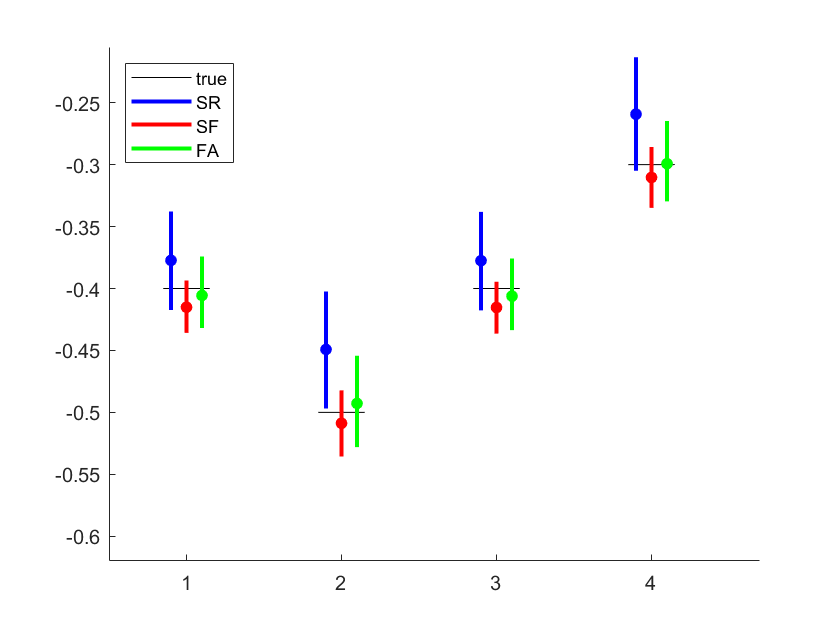
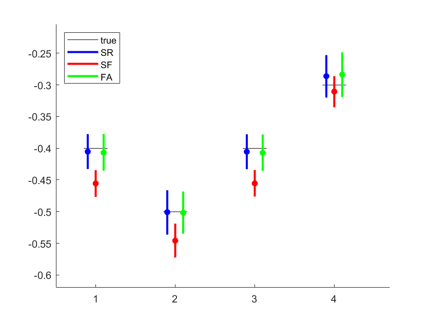
Figure 1: True and estimated in-sample average treatment effects (including 95%-HPD intervals) for the various models. Data simulated from the shared factor model (left) and the switching regression model (right).

To illustrate the flexibility of the proposed FA treatment effects model, we analyse two data sets introduced in Jacobi et al. (2016), which were simulated from the shared factor model (SF) and the switching regression model (SR), respectively, with parameters that violate assumptions of the respective alternative model. Each data set contains a panel of length $T=4$ of the observed outcome of $n=50,000$ subjects where the large number of subjects was chosen to illustrate the bias in the average treatment estimates resulting from miss-specification of the correlation structure. For both data sets the probit model and the mean structure of the two potential outcomes models as well as the error variances $\boldsymbol{\sigma}_{0}$ and $\boldsymbol{\sigma}_{1}$ where specified to be identical (see Jacobi et al. (2016) for details), the two data sets however differed with respect to the correlation structure of the latent utility and the two potential outcomes sequences.

Both data sets were analysed using a shared factor model, a switching regression model and a factor-augmented model (FA). An estimate for the average treatment effects in panel period $t$, $\text{ATE}_{t}$, over all subjects was obtained as

$$\widehat{\text{ATE}}_{t}=\hat{\kappa}_{t}+\frac{1}{n}\sum_{i=1}^{n}\mathbf{w}_{it}\hat{\boldsymbol{\theta}},$$

based on the estimated posterior means of the regression effects $\hat{\boldsymbol{\theta}}$ and $\hat{\kappa}_{t}$ in the potential outcomes models.

Figure 1 shows for $t=1,\dots,4$ the true average treatment effect and the estimated average treatment effects under each model with the 95%-HPD intervals. These intervals do not include the true average treatment effect at all time points if data generated from the SF model are analysed with the SR model or, vice-versa, data generated from the SR model are analysed with the SF model. In contrast, in both cases the proposed factor-augmented model covers the true treatment effects and performs similar as the respective data generating model.

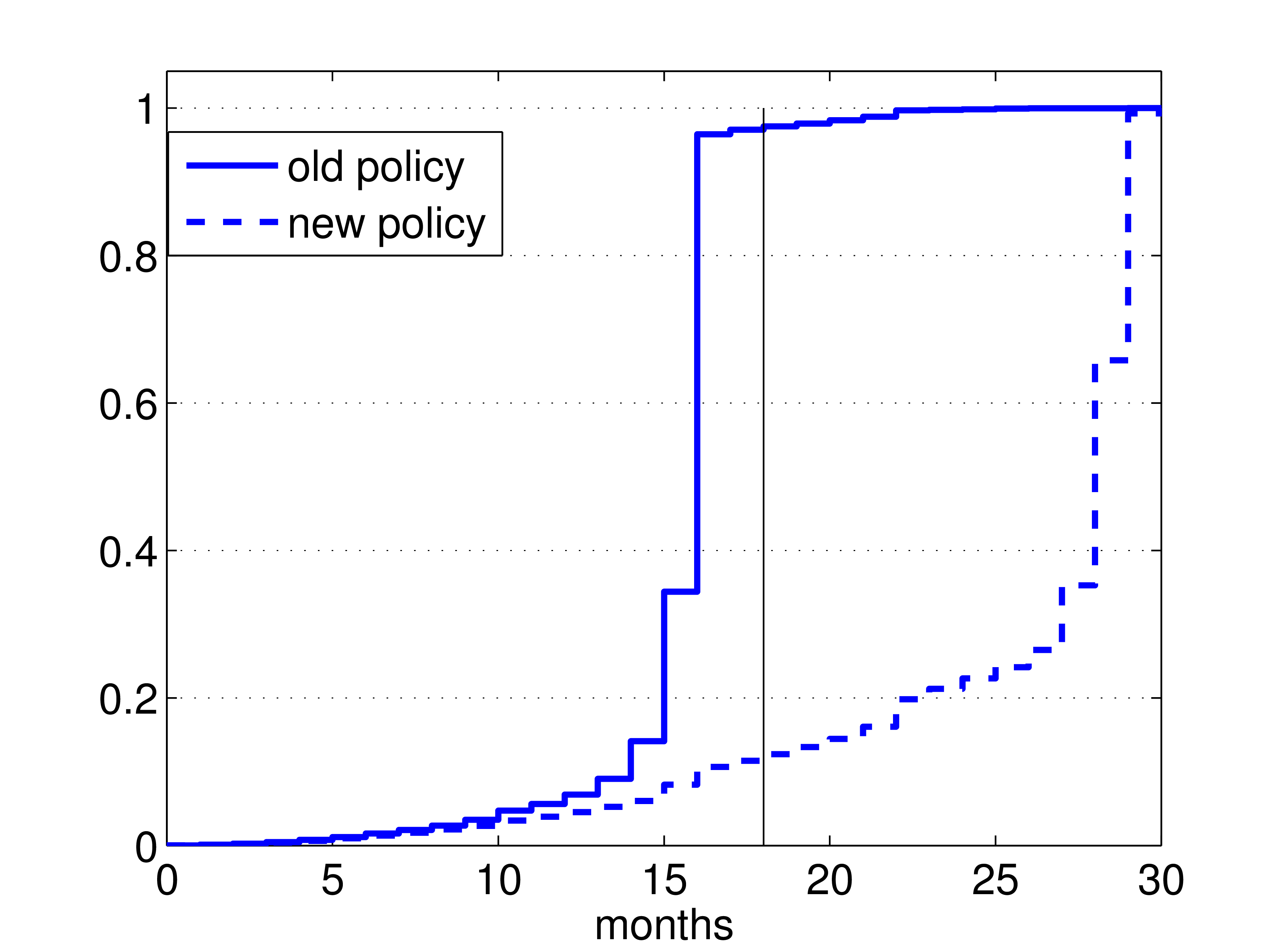
Figure 2: Empirical cdf of the duration of maternity leave after child birth

5 Analysing Earnings Effects of Maternity Leave

We apply the factor-augmented model to re-analyse the effects of a long maternity leave on earnings of Austrian mothers after their return to the labor market using the same data as Jacobi et al. (2016). The analysis is based on data from the Austrian Social Security Data Base (ASSD), which is an administrative data set of the universe of Austrian employees providing detailed information on employment and maternity leave spells as well as demographic information on mothers (Zweimüller et al., 2009).

To exploit a change in the parental leave policy in Austria in July 2000 which extended the payment of parental leave benefits from 18 to 30 months, Jacobi et al. (2016) used data for mothers who gave birth to their last child from June 1998 till July 2002. Figure 2 illustrates that the majority of mothers returned to the labour market within 18 months before this policy change whereas afterwards most mothers took a longer maternity leave of more than 18 months.

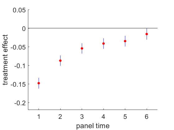
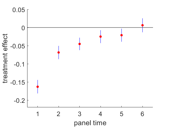
Figure 3: Estimated average treatment effects and 95%-HPD-intervals of a long maternity leave. Analysis with the shared factor model (SF, left), the switching regression model (SR, middle) and the factor-augmented model (FA, right).

Jacobi et al. (2016) defined treatment as a maternity leave longer than 18 months. Based on a shared factor model as well as a switching regression model, they analysed the treatment effect on earnings for those mothers who returned to the labour market immediately after the end of the maternity leave. We use the same specification for the mean of the latent utility and the potential outcomes, defined as the log income, as in their analysis, but model the joint distribution of the errors $\boldsymbol{\varepsilon}_{i}$ by the factor-augmented model proposed in this paper.

Figure 3 compares the average treatment effects over all mothers in the sample for the first 6 years after returning to the labour market, estimated by these three models. For all models, a long maternity leave results in considerably lower earnings in the first panel period with the gap decreasing over time. However, the evolvement of $\widehat{\text{ATE}}_{t}$ is slightly different for the three models: it is still negative in panel period 6 for the shared factor model, positive for the switching regression model and practically zero for the factor-augmented model. Detailed estimation results are provided in Appendix C in Table 1, Table 2 and Table 3.

6 Conclusion

Inference on treatment effects for longitudinally observed outcomes can be biased when the model used for data analyses implies restrictions on the association between selection into treatment and the potential outcomes sequences as well as within the potential outcomes sequences which are violated for the data to be analysed. The proposed factor-augmented model explicitly models these associations by latent factors and hence is more flexible than the models used so far. However, as the two potential outcomes sequences are never observed together, only the fit of the probit model for the latent utility and the marginal models for the potential outcomes can be assessed, but not the implied association of the two potential outcomes.

Appendix A Moments of the observed outcomes

To derive the first two moments of the observed outcomes we start with a univariate normal random variable $Z\sim\mathcal{N}\left(\mu,\sigma^{2}\right)$, and then consider the $(T+1)$-variate normal random variable $(x^{*},\mathbf{y})^{\prime}$.

Expectation and variance of $Z$ truncated to $(a,b)$ are given as

$$\operatorname{E}(Z|a<Z<b) =\mu-\sigma\frac{\phi(\frac{b-\mu}{\sigma})-\phi(\frac{a-\mu}{\sigma})}{\Phi(\frac{b-\mu}{\sigma})-\Phi(\frac{a-\mu}{\sigma})},$$

$$\operatorname{V}(Z|a<Z<b) =\sigma^{2}\left[1-\frac{1}{\sigma}\frac{(b-\mu)\phi(\frac{b-\mu}{\sigma})-(a-\mu)\phi(\frac{a-\mu}{\sigma})}{\Phi(\frac{b-\mu)}{\sigma}-\Phi(\frac{a-\mu}{\sigma})}-\Big{(}\frac{\phi(\frac{b-\mu}{\sigma})-\phi(\frac{a-\mu}{\sigma})}{\Phi(\frac{b-\mu}{\sigma})-\Phi(\frac{a-\mu}{\sigma})}\Big{)}\right]^{2}.$$

Let $(x^{*},\mathbf{y})^{\prime}\sim\mathcal{N}\left(\boldsymbol{\mu},\boldsymbol{\Sigma}\right)$ with moments

$$\boldsymbol{\mu}=\begin{pmatrix}\mu_{x}\\ \boldsymbol{\mu}_{\mathbf{y}}\end{pmatrix}\quad\text{and}\quad\boldsymbol{\Sigma}=\begin{pmatrix}\sigma^{2}_{x}&\boldsymbol{\sigma}_{x\mathbf{y}}^{\prime}\\ \boldsymbol{\sigma}_{x\mathbf{y}}&\boldsymbol{\Sigma}_{\mathbf{y}}\end{pmatrix}.$$

The conditional distribution of $\mathbf{y}|x^{*}$ is given as

$$\mathbf{y}|x^{*}\sim\mathcal{N}\left(\boldsymbol{\mu}_{\mathbf{y}}+\frac{\boldsymbol{\sigma}_{x\mathbf{y}}}{\sigma_{x}^{2}}(x^{*}-\mu_{x}),\boldsymbol{\Sigma}_{\mathbf{y}}-\frac{\boldsymbol{\sigma}^{\prime}_{x\mathbf{y}}\boldsymbol{\sigma}_{x\mathbf{y}}}{\sigma^{2}_{x}}\right),$$

and interest is in the first two moments of $\mathbf{y}|(x^{*}<0)$ as well as those of $\mathbf{y}|(x^{*}>0)$.

The conditional expectation $\operatorname{E}(\mathbf{y}|x^{*}<0)$ results as

$$\operatorname{E}(\mathbf{y}|x^{*}<0)=\boldsymbol{\mu}_{\mathbf{y}}+\frac{\boldsymbol{\sigma}_{x\mathbf{y}}}{\sigma_{x}^{2}}\operatorname{E}(x^{*}-\mu_{x}|x^{*}<0)=\boldsymbol{\mu}_{\mathbf{y}}-\frac{\boldsymbol{\sigma}_{x\mathbf{y}}}{\sigma_{x}}\frac{\phi(\mu_{x}/\sigma_{x})}{1-\Phi(\mu_{x}/\sigma_{x})}.$$

The conditional second moment of $(\mathbf{y}-\boldsymbol{\mu}_{\mathbf{y}})|(x^{*}<0)$ can be derived as

$$\operatorname{E}((\mathbf{y}-\boldsymbol{\mu}_{\mathbf{y}})(\mathbf{y}-\boldsymbol{\mu}_{\mathbf{y}})^{\prime}|x^{*}<0)=\boldsymbol{\Sigma}_{\mathbf{y}}-\frac{\boldsymbol{\sigma}^{\prime}_{x\mathbf{y}}\boldsymbol{\sigma}_{x\mathbf{y}}}{\sigma^{2}_{x}}+\frac{\boldsymbol{\sigma}^{\prime}_{x\mathbf{y}}\boldsymbol{\sigma}_{x\mathbf{y}}}{\sigma^{4}_{x}}\operatorname{E}\big{(}(x^{*}-\mu_{x})^{2}|x^{*}<0),$$

and, hence, the conditional covariance matrix $\operatorname{V}(\mathbf{y}|x^{*}<0)$ is given as

$$\operatorname{V}(\mathbf{y}|x^{*}<0) =\boldsymbol{\Sigma}_{\mathbf{y}}-\frac{\boldsymbol{\sigma}^{\prime}_{x\mathbf{y}}\boldsymbol{\sigma}_{x\mathbf{y}}}{\sigma_{x}^{2}}+\frac{\boldsymbol{\sigma}^{\prime}_{x\mathbf{y}}\boldsymbol{\sigma}_{x\mathbf{y}}}{\sigma_{x}^{2}}\operatorname{V}(x^{*}|x^{*}<0)$$

$$=\boldsymbol{\Sigma}_{\mathbf{y}}+\frac{\boldsymbol{\sigma}^{\prime}_{x\mathbf{y}}\boldsymbol{\sigma}_{x\mathbf{y}}}{\sigma_{x}^{2}}\Big{(}\frac{\mu_{x}}{\sigma_{x}}\frac{\phi(\mu_{x}/\sigma_{x})}{1-\Phi(\mu_{x}/\sigma_{x})}-\big{(}\frac{\phi(\mu_{x}/\sigma_{x})}{1-\Phi(\mu_{x}/\sigma_{x})})^{2}\Big{)}.$$

Similarly, expectation and covariance of $\mathbf{y}|(x^{*}>0)$ can be derived as

$$\operatorname{E}(\mathbf{y}|x^{*}>0) =\boldsymbol{\mu}_{\mathbf{y}}+\frac{\boldsymbol{\sigma}_{x\mathbf{y}}}{\sigma_{x}}\frac{\phi(\mu_{x}/\sigma_{x})}{\Phi(\mu_{x}/\sigma_{x})}$$

$$\operatorname{V}(\mathbf{y}|x^{*}>0) =\boldsymbol{\Sigma}_{\mathbf{y}}-\frac{\boldsymbol{\sigma}^{\prime}_{x\mathbf{y}}\boldsymbol{\sigma}_{x\mathbf{y}}}{\sigma^{2}_{x}}\Big{(}\frac{\mu_{x}}{\sigma_{x}}\frac{\phi(\mu_{x}/\sigma_{x})}{\Phi(\mu_{x}/\sigma_{x})}+\big{(}\frac{\phi(\mu_{x}/\sigma_{x})}{\Phi(\mu_{x}/\sigma_{x})})^{2}\Big{)}.$$

Appendix B MCMC scheme

With starting values for $\boldsymbol{\alpha},\boldsymbol{\beta},\boldsymbol{\zeta},\boldsymbol{\lambda}$ and all latent factors MCMC is performed by iterating the following steps:

1. Sample the idiosyncratic variances $\boldsymbol{\sigma}^{2}_{0}$ and $\boldsymbol{\sigma}^{2}_{1}$. For $j=0,1$ and $t=1,\dots,T$ sample $\sigma_{jt}^{2}$ from $\mathcal{G}^{-1}\left(s_{n,jt},S_{n,jt}\right)$ where

   $$s_{n,jt}=s_{0,jt}+n_{jt}/2,\qquad S_{n,jt}=S_{0,jt}+Se_{jt}/2,$$

   and

   $$Se_{jt}=\sum_{i:x_{i}=j}(y_{j,it}-\mathbf{w}_{j,it}\boldsymbol{\beta}-f_{ci}\lambda_{jt}-f_{ji}\zeta_{j,t})^{2}.$$

   Here $n_{jt}$ is the number of subjects for which $y_{j,it}$ is observed and $\mathbf{w}_{j,it}$ denotes the values of the covariates at panel time $t$, i.e. row $t$ of the covariate matrix $\mathbf{W}_{ji}$.

2. Sample the latent factors. For $i=1,\dots,n,$ sample the latent factor $f_{ci}$ and the specific factor $f_{ji}$ for $x_{i}=j$ from the full conditional posterior

   $$p(f_{ci},f_{ji}|\boldsymbol{\Theta},x_{i}^{*},\mathbf{y}_{x_{i},i})\propto p(x^{*}_{i},\mathbf{y}_{x_{i},i}|\boldsymbol{\Theta},f_{ci})p(f_{ci},f_{ji})$$

   For $x_{i}=j$, the errors of latent utility $x^{*}_{i}$ and the outcome vector $\mathbf{y}_{ji}$ are given as

   $$\varepsilon_{xi} =x^{*}_{i}-\mathbf{v}_{i}\boldsymbol{\alpha}=\lambda_{x}f_{ci}+\epsilon_{xi},$$

   $$\boldsymbol{\varepsilon}_{ji} =\mathbf{y}_{ji}-\mathbf{W}_{i}\boldsymbol{\beta}=\boldsymbol{\lambda}_{j}f_{ci}+\boldsymbol{\zeta}_{j}f_{ji}+\boldsymbol{\epsilon}_{ji},$$

   and hence the full conditional of $(f_{ci},f_{ji})$ is a bivariate normal distribution, $\mathcal{N}\left(\mathbf{f}_{n,i},\mathbf{F}_{n,i}\right)$. With

   $$\boldsymbol{\Psi}_{j}=\begin{pmatrix}\lambda_{x}&0\\ \boldsymbol{\lambda}_{j}&\boldsymbol{\zeta}_{j}\end{pmatrix}\qquad\text{and}\qquad\tilde{\mathbf{S}_{j}}=\operatorname{diag}(\sigma^{2}_{x},\boldsymbol{\sigma}_{j}),$$

   the posterior moments are given as

   $$\mathbf{F}_{n,i} =(\boldsymbol{\Psi}_{j}^{\prime}\tilde{\mathbf{S}_{j}}^{-1}\boldsymbol{\Psi}_{j}+\mathbf{I}_{2})^{-1},$$

   $$\mathbf{f}_{n,i} =\mathbf{F}_{n,i}\boldsymbol{\Psi}_{j}^{\prime}\tilde{\mathbf{S}_{j}}^{-1}\begin{pmatrix}\varepsilon_{xi}\\ \boldsymbol{\varepsilon}_{ji}\end{pmatrix}.$$

3. Sample the latent utilities $x^{*}_{i}$. For $i=1,\dots,n$ sample $x^{*}_{i}$ from $\mathcal{N}\left(\mathbf{v}_{i}\boldsymbol{\alpha}+\lambda_{x}f_{ci},1\right)$ truncated to the interval $(-\infty,0)$ for $x_{i}=0$ and to $(0,\infty)$ if $x_{i}=1$.

4. Sample the parameters in the selection equation. The selection equation for $x_{i}^{*}$, $i=1,\dots,n$, is given as

   $$x_{i}^{*}=\mathbf{v}_{i}\boldsymbol{\alpha}+f_{ci}\lambda_{x}+\epsilon_{xi},\quad\epsilon_{xi}\sim\mathcal{N}\left(0,1\right).$$

   $f_{ci}$ is mandatorily included in the model and therefore only elements of $\boldsymbol{\alpha}$ are subject to variable selection, but $\lambda_{x}$ is not.

5. Sample the parameters of the outcome equation. The model for the observed outcomes $\mathbf{y}_{x_{i},i}$, $i=1,\dots,n$ is given as

   $$\mathbf{y}_{x_{i},i}=\mathbf{W}_{x_{i},i}\boldsymbol{\beta}+f_{ci}\boldsymbol{\lambda}_{x_{i}}+f_{x_{i},i}\boldsymbol{\zeta}_{x_{i}}+\boldsymbol{\epsilon}_{x_{i},i},\quad\boldsymbol{\epsilon}_{x_{i},i}\sim\mathcal{N}\left(\mathbf{0},\boldsymbol{\Sigma}_{x_{i}}\right).$$

   Also in the outcome equation, variable selection is implemented only for the elements of $\boldsymbol{\beta}$, but not for the factor loadings $\boldsymbol{\lambda}_{x_{i}}$ and $\boldsymbol{\zeta}_{x_{i}}$

6. Boosting. Perform boosting based on marginal data augmentation as described in Frühwirth-Schnatter and Lopes (2018) and a sign-switch for the factor loadings and the respective factor. For the sign-switch, $\tau_{c}$, $\tau_{0}$, and $\tau_{1}$ are sampled independently from $\{-1,1\}$ and

   $$\boldsymbol{\lambda} =\tau_{c}\boldsymbol{\lambda},\quad f_{ci}=\tau_{c}\boldsymbol{\lambda},\quad i=1,\dots,n,$$

   $$\boldsymbol{\lambda} =\tau_{j}\boldsymbol{\zeta},\quad f_{ji}=\tau_{j}\boldsymbol{\lambda},\quad i=1,\dots,n.$$

7. Sample the inclusion probabilities. Sample $\pi_{\alpha}|k_{\alpha}$ from $\mathcal{B}\left(1+k_{\alpha},1+d_{\alpha}-k_{\alpha}\right)$ and $\pi_{\beta}|k_{\beta}$ from $\mathcal{B}\left(1+k_{\beta},1+d_{\beta}-k_{\beta}\right)$ where $k_{\alpha}=\sum\delta^{\alpha}_{\ell}$ is the number of selected regressors for the latent utility and $k_{\beta}=\sum\delta^{\beta}_{\ell}$ accordingly the number of selected regressors for the potential outcome equations.

Sampling steps (4) and (5) are standard sampling steps in linear regression models with variable selection, see Jacobi et al. (2016) for details.

	mean	sd	prob
intercept	-1.562	0.032	—
z	2.827	0.021	1.000
child 2	0.052	0.036	0.737
child $>3$	-0.012	0.032	0.157
exp	0.093	0.027	0.985
blue collar	-0.059	0.044	0.706
int. exp/blue	-0.016	0.040	0.177
base-earn Q2	0.002	0.012	0.060
base-earn Q3	-0.001	0.008	0.035
base-earn Q4	-0.153	0.027	1.000

Table 1: Results selection equation: posterior means (mean), standard deviation (sd, in parentheses) and estimated posterior inclusion probabilities (prob.) of standardized regression effects

Appendix C Results of the FA model for the mother data

The data set contains information on 31,051 mothers with earnings after return to labor market observed over 4-6 consecutive panel periods. Covariates are specified as in the analysis of Jacobi et al. (2016). Covariates included in the selection equation are an indicator for the policy change (z=1 indicates longer payment of parental leave benefits), indicator variables for the child (child2=1 if the mother has already an child and child $>3$ =1 if the mother has 2 or more older children), the working experience (exp=1 if the working experience is above the median working experience in the sample), type of contract (blue collar or white collar) and the interaction between these two and finally indicators to control for earnings before the first child in terms of quartiles. The outcome model additionally includes indicator variables for panel periods 2-6 and for return to the same employer (eq.emp) and a quadratic calendar year effect.

MCMC estimation as outlined in Appendix B was run for 500000 iteration after a burn-in of 10000 with variable selection starting after 5000 iterations of the burn-in. To determine posterior mean estimates we applied a thinning of 500.

	treatment 0		treatment 1
	mean   (sd)	prob	mean   (sd)	prob
intercept	9.309   (0.014)	—	-0.130   ( 0.011)	1.000
child 2	-0.000   (0.001)	0.008	-0.000   ( 0.001)	0.011
child $>$3	0.000   (0.001)	0.014	0.000   (0.002)	0.021
exp	-0.092   (0.010)	1.000	0.011   ( 0.015)	0.388
blue collar	-0.108   (0.006)	1.000	0.000   ( 0.002)	0.015
int. exp/blue	0.001   (0.004)	0.039	0.005   ( 0.012)	0.173
base-earn Q2	0.066   (0.006)	1.000	0.000   ( 0.002)	0.016
base-earn Q3	0.286   (0.011)	1.000	-0.047   ( 0.014)	0.974
base-earn Q4	0.606   (0.010)	1.000	-0.116   ( 0.013)	1.000
eq. emp	0.049   (0.005)	1.000	0.000   ( 0.003)	0.031
panel $t=2$	0.066   (0.004)	1.000	0.068   ( 0.004)	1.000
panel $t=3$	0.106   (0.006)	1.000	0.115   ( 0.006)	1.000
panel $t=4$	0.149   (0.009)	1.000	0.141   ( 0.008)	1.000
panel $t=5$	0.201   (0.011)	1.000	0.151   ( 0.009)	1.000
panel $t=6$	0.252   (0.013)	1.000	0.163   ( 0.010	1.000
$(year-1999)$	0.050   (0.005)
$(year-1999)^{2}$	-0.005   (0.000)

Table 2: Results outcome equation: posterior means (mean), standard deviation (sd, in parentheses) and estimated posterior inclusion probabilities (prob.) of regression effects

Table 1 reports results for the standardized estimated effects $\tilde{\boldsymbol{\alpha}}$. The factor loading of the common factor in the selection equation is $\hat{\lambda}_{x}=0.277$ (sd=0.014). Estimation results for the regression effects in the outcome equation are given in Table 2 and for the factor loadings and idiosyncratic variances in Table 3.

	treatment 0			treatment 1
t	$\boldsymbol{\lambda}_{0}$	$\boldsymbol{\zeta}_{0}$	$\boldsymbol{\sigma}_{0}^{2}$	$\boldsymbol{\lambda}_{1}$	$\boldsymbol{\zeta}_{1}$	$\boldsymbol{\sigma}_{1}^{2}$
1	-0.296 (0.017)	0.254 (0.019)	0.088 (0.001)	0.327 (0.005)	0.038 (0.028)	0.078 (0.001)
2	-0.334 (0.019)	0.284 (0.022)	0.025 (0.001)	0.385 (0.009)	0.068 (0.039)	0.016 (0.001)
3	-0.377 (0.012)	0.183 (0.024)	0.038 (0.001)	0.340 (0.020)	0.171 (0.038)	0.023 (0.000)
4	-0.412 (0.006)	0.083 (0.026)	0.032 (0.000)	0.288 (0.031)	0.271 (0.032)	0.019 (0.000)
5	-0.434 (0.003)	0.023 (0.016)	0.012 (0.000)	0.248 (0.035)	0.310 (0.027)	0.023 (0.001)
6	-0.415 (0.003)	0.022 (0.016)	0.032 (0.001)	0.231 (0.035)	0.308 (0.026)	0.037 (0.001)

Table 3: Results factor loadings and idiosyncratic variances: posterior means (mean) and standard deviations (sd, in parentheses)

References

- Anderson and Rubin (1956) T. W. Anderson and Herman Rubin. Statistical inference in factor analysis. In Proceedings of the Third Berkeley Symposium on Mathematical Statistics and Probability, volume V, pages 111–150, 1956.
- Carneiro et al. (2003) P. Carneiro, Karsten T. Hansen, and James J. Heckman. Estimating distributions of treatment effects with an application to the returns to schooling and measurement of the effects of uncertainty of college choice. International Economic Review, 44:361–422, 2003.
- Chib and Jacobi (2007) Siddhartha Chib and Liana Jacobi. Modeling and calculating the effect of treatment at baseline from panel outcomes. Journal of Econometrics, 140:781–801, 2007.
- Conti et al. (2014) G. Conti, S. Frühwirth-Schnatter, J. J. Heckman, and R. Piatek. Bayesian exploratory factor analysis. Journal of Econometrics, 183:31–57, 2014.
- Frühwirth-Schnatter and Lopes (2018) Sylvia Frühwirth-Schnatter and Hedibert Lopes. Sparse Bayesian Factor Analysis when the Number of Factors is Unknown. 2018. arXiv preprint 1804.04231.
- Holzinger and Swineford (1937) K. J. Holzinger and F. Swineford. The bi-factor method. Psychometrika, 2:41–54, 1937.
- Jacobi et al. (2016) L. Jacobi, H. Wagner, and S. Frühwirth-Schnatter. Bayesian treatment effects models with variable selection for panel outcomes with an application to earnings effects of maternity leave. Journal of Econometrics, 193:234–250, 2016.
- Lee (1978) L.-F. Lee. Unionism and wage rates: A simultaneous equations model with qualitative and limited dependent variables. International Economic Review, 19:415–433, 1978.
- Reise (2012) S. P. Reise. The rediscovery of bifactor measurement models. Multivariate Behavioural Research, 47:667–696, 2012.
- Roy (1951) A. D. Roy. Some thoughts on the disitribution of earnings. Oxford Economic Papers, 3:135–146, 1951.
- Rubin (1981) Donald B. Rubin. Estimation in parallel randomized experiments. Journal of Educational Statistics, 6:377–401, 1981.
- Zweimüller et al. (2009) Josef Zweimüller, Rudolf Winter-Ebmer, Rafael Lalive, Andreas Kuhn, Jean-Philipe Wuellrich, Oliver Ruf, and Simon Büchi. The Austrian Social Security Database (ASSD). Working Paper 0903, NRN: The Austrian Center for Labor Economics and the Analysis of the Welfare State, Linz, Austria, 2009.