Projective measurements under qubit quantum channels

Abstract

The action of qubit channels on projective measurements on a qubit state is used to establish an equivalence between channels and properties of generalized measurements characterized by bias and sharpness parameters. This can be interpreted as shifting the description of measurement dynamics from the Schrodinger to the Heisenberg picture. In particular, unital quantum channels are shown to induce unbiased measurements. The Markovian channels are found to be equivalent to measurements for which sharpness is a monotonically decreasing function of time. These results are illustrated by considering various noise channels. Further, the effect of bias and sharpness parameters on the energy cost of a measurement and its interplay with non-Markovianity of dynamics is also discussed.

I Introduction

Measurement in quantum theory plays a crucial role compared to its classical counterpart. The ineluctable feature of any quantum measurement is that it entails an interaction between the measuring apparatus so that the observed system necessarily gets entangled with the system of observing apparatus Busch et al. (1996); Braginsky et al. (1992). The text-book description of quantum measurement usually deals with the ideal measurement when there is an one-to-one correspondence between system and apparatus states is achieved. Such an ideal measurement scenario can be modelled by a complete set of orthogonal projectors on the given Hilbert space of the system. However, in practice, the system-apparatus correspondence may not be achieved in general measurement scenario. In such a case, the orthogonal projectors are needed to be replaced by the so-called positive operator-valued measures (POVMs) which is a set of Hermitian, positive semi-definite operators commonly denoted as $\{E_{i}\}$, that sum up to identity, i.e., $\sum_{i=1}^{n}E_{i}=\mathbb{1}$. If all the elements of a POVM are projective, i.e., $E_{i}=\Pi_{i}=\ket{\phi_{i}}\bra{\phi_{i}}$, where $\{\ket{\phi_{i}}\}$ is an orthonormal basis, then the measurement is called sharp. There are pertinent schemes where the generalized measurement involving POVMs outperform the projective measurements, such as, quantum tomography Braginsky et al. (1992), unambiguous state discrimination Busch and Schmidt (2010), quantum cryptography Yu et al. (2010); Busch and Jaeger (2010); Das et al. (2018), device-independent randomness certification Acín et al. (2016) and many more.

Mathematically, a two-outcome POVMs in two dimension in its general form can be written as Busch and Schmidt (2010); Stano et al. (2008); Yu et al. (2010)

$$E_{\pm}(x,\vec{m})=\frac{\mathbb{1}\pm(\mathbb{1}x+\vec{m}\cdot\vec{\sigma})}{2}.$$ (1)

where $x$ and $|\vec{m}|$ are called bias and sharpness parameters respectively. The positivity of the POVMs $E_{\pm}(x,\vec{m})$ demands that the following condition be satisfied

$$|x|+|\vec{m}|\leq 1.$$ (2)

For ideal sharp measurement scenario, $|x|=0$ and $|\vec{m}|=1$. The notion of bias and shapness capture the deviation from the ideal projective measurements, but arises due to different physical reasons. The sharpness parameter is linked with the precision of measurement arising due to operational indistinguishability between the probability distributions corresponding to the post-measurement apparatus states and thus $|\vec{m}|=1$ implies vanishingly small overlap between them. On the other hand bias parameter quantifies the tendency of a measurement to favor one state over the other. When $|x|=0$ the POVM $E_{\pm}(0,\vec{m})$ is called unbiased, meaning that the outcomes of measurement are purely random if the system is prepared in a maximally mixed state, i.e., $\operatorname{Tr}\{E_{+}(0,\vec{m})\mathbb{1}/2\}=\operatorname{Tr}\{E_{-}(0,\vec{m})\mathbb{1}/2\}=1/2$.

The POVM elements in Eq. (1), can be viewed as an affine transformation on a pure state $\rho=\frac{1}{2}(\mathbb{1}+\vec{r}\cdot\sigma)$, with $\vec{r}=(\sin\theta\cos\phi,\sin\theta\sin\phi,\cos\theta)$ being the Bloch vector. The post-measurement state becomes $\rho^{\pm}=\frac{1}{2}(\mathbb{1}+\vec{s}^{\pm}\cdot\sigma)$, such that

$$\vec{s}^{\pm}=A^{\pm}\vec{r}+\vec{T}^{\pm}.$$ (3)

Here, $A_{ij}^{\pm}=\frac{1}{2}\operatorname{Tr}\{\sigma_{i}E_{\pm}[\sigma_{j}]\}$ and $T_{i}^{\pm}=\frac{1}{2}\operatorname{Tr}\{\sigma_{i}E_{\pm}[\mathbb{1}]\}$, with $E_{j}[\bm{\omega}]=E_{j}\bm{\omega}E_{j}^{\dagger}$, $j=\pm$. We have

$$A_{ii}^{\pm} =\frac{1}{4}\big{[}(1\pm x)^{2}+2m_{i}^{2}-|\vec{m}|^{2}\big{]},$$ (4)

$$A_{ij}^{\pm} =\frac{m_{i}m_{j}}{2},~{}~{}{\rm for}~{}~{}i\neq j;\ \ T_{i}^{\pm}=\frac{m_{i}}{2}(1+x),$$

with $i,j=1,2,3$ and $\pm$ pertaining to the POVM element $E_{\pm}$ being used.

The effect of biased-unsharp measurements on various quantum correlations has been studied in Busch and Jaeger (2010); Das et al. (2018); Kumari and Pan (2017). The biased and unsharp measurements have been realized experimentally using quantum feedback stabilization of photon number in a cavity Sayrin et al. (2011). The unsharp measurements were studied with qubit observables through an Arthur–Kelly-type joint measurement model for qubits Pal and Ghosh (2011). Recently, implementation of generalized measurements on a qudit via quantum walks was also proposed Li et al. (2019).

The quantum dynamics, in its idealized version without presence of environment, is governed by unitary evolution. In realistic scenario, the most general evolution is governed by quantum channels which are characterized by suitably formulated Kraus operators. The action of a quantum channel is conveniently studied in the Schrödinger picture, while its effect on the operator, leading to the operators subsequent evolution, requires the use of the Heisenberg picture. In this work, we address the following issues. Under the action of a quantum dynamical process (e.g., a quantum channel), how does an ideal projector evolve, and whether such a process transform it to a POVM. In particular, we examine the types of quantum channels that leads to the two-outcome biased-unsharp POVMs. Moreover, we have investigated the behavior of the bias and sharpness parameters under the effect of Markovian as well as non-Markovian nature of the quantum dynamics. Further, in a direction towards motivating our study, we look at the comparison of energy costs for implementing such measurements under different kinds of open system dynamics.

The work is organized as follows: In Sec. (II) we start with a brief review of quantum channels and discuss the effect of dynamics on ideal measurements. The arguments are made rigorous by proving two theorems establishing that the conjugate of a unital (non-unital) channel generates unbiased (biased) POVM. Also, the conjugate of a Markovian channel is shown to lead to unsharp measurements such that the sharpness is a monotonically decreasing function of time. The effect of bias and sharpness, in the context of non-Markovian dynamics, on the energy cost of measurements is discussed in Sec. (III). We conclude in Sec. (IV).

II Quantum channels and biased-unsharp POVMs

Mathematically, quantum channels are linear maps $\mathcal{E}:\mathcal{S}(X)\rightarrow\mathcal{S}(Y)$, such that $\mathcal{S}(X)$ ($\mathcal{S}(Y)$) is the set of all density operators acting on $X$ ($Y$) Watrous (2018). Geometrically, the quantum channel $\mathcal{E}$ is an affine transformation Ruskai et al. (2002). An elegant description of quantum channels is given in terms of operator sum representation, such that an initial density matrix $\rho$ is evolved to some final density matrix $\rho^{\prime}$

$$\rho^{\prime}=\mathcal{E}[\rho]=\sum\limits_{i}\mathcal{K}_{i}\rho\mathcal{K}_{i}^{\dagger}.$$ (5)

Here $\mathcal{K}_{i}$ are the Kraus operators and satisfy the completeness condition $\sum_{i}\mathcal{K}_{i}^{\dagger}\mathcal{K}_{i}=\mathbb{1}$. The conjugate channel $\mathcal{E}^{\dagger}$ corresponding to $\mathcal{E}$ is defined such that $\mathcal{E}^{\dagger}[\rho]=\sum\limits_{i}\mathcal{K}_{i}^{\dagger}\rho\mathcal{K}_{i}$.

An important class of quantum channels are the unital channels, each of which maps Identity operator to itself, that is, $\mathcal{U}[\mathbb{1}]=\mathbb{1}$. Examples include the phase damping, depolarizing and Pauli channels Banerjee and Ghosh (2007); Omkar et al. (2013). A typical example of non-unital channel is the amplitude damping channel Banerjee (2018); Srikanth and Banerjee (2008); Banerjee and Srikanth (2008). Note that the conjugate channel of each quantum channel is unital. For unital qubit channels, the following properties are equivalent Mendl and Wolf (2009):

1. $\mathcal{E}$ is unital if $\mathcal{E}[\mathbb{1}]=\mathbb{1}$.

2. $\mathcal{E}$ can be realized as a random unitary map: ${\cal E}(\rho)=\sum_{i}p_{i}U_{i}\rho U_{i}^{\dagger}$ with $U_{i}$’s being unitary and $p_{i}$’s being probabilities such that $\sum_{i}p_{i}=1$.

The projective measurements are mapped to the POVMs due to the action of channels. As an example, consider a unital qubit channel $T$ which can be described as Mendl and Wolf (2009) $T(\rho)=\sum_{i}\lambda_{i}U^{\dagger}_{i}\rho U_{i}=\rho^{\prime}$, with $U_{i}U_{i}^{\dagger}=\mathbb{1}$, and $\sum_{i}\lambda_{i}=1$. Let a qubit projective measurement be denoted by $\Pi^{\pm}$ such that the probability of obtaining the outcome $\pm 1$ is given by $\rm{prob}({\pm}1)=\operatorname{Tr}\{\Pi^{\pm}\rho^{\prime}\}=\operatorname{Tr}\{\Pi^{\pm}\sum_{i}\lambda_{i}U^{\dagger}_{i}\rho U_{i}\}=\operatorname{Tr}\{\sum_{i}\lambda_{i}U_{i}\Pi^{\pm}U^{\dagger}_{i}\rho\}=\operatorname{Tr}\{E_{\pm}\rho\}$. Here $E_{\pm}=\sum_{i}\lambda_{i}U_{i}\Pi^{\pm}U^{\dagger}_{i}$ can be identified as the POVM elements, in the sense that the projectors evolve to POVMs: $E_{\pm}\geq 0$ and $E_{+}+E_{-}=I$, through the dynamics. Since $\Pi^{\pm}$ is a projector having unit trace, therefore $\operatorname{Tr}\{U_{i}\Pi^{\pm}U^{\dagger}_{i}\}=1$, as $U_{i}$ is trace preserving. This indicates that $\operatorname{Tr}\{E_{\pm}\}=\operatorname{Tr}\{\sum_{i}\lambda_{i}U_{i}\Pi^{\pm}U^{\dagger}_{i}\}=\sum_{i}\lambda_{i}\operatorname{Tr}\{U_{i}\Pi^{\pm}U^{\dagger}_{i}\},=\sum_{i}\lambda_{i}=1$. But, the trace of POVM element $E_{\pm}$ in Eq. (1) is $\operatorname{Tr}\{E_{\pm}\}=\operatorname{Tr}\{\frac{\mathbb{1}\pm(\mathbb{1}x+\vec{m}.\vec{\sigma})}{2}\}=1\pm x$. Hence a unital qubit channel acting on projectors leads to unbiased POVMs.

Table 1: The bias and sharpness parameters corresponding to different noise channels. Here, $\Theta$ is the measurement parameter defined in Eq. (8). Detailed discussion about these channels (including their time dependence) can be found in the cited references.

Channel (unital/non-unital)	Kraus operators	Bias	Sharpness
Random Telegraph Noise (RTN) Daffer et al. (2004), unital, with memory	$R_{1}=\sqrt{\frac{1+\Lambda(t)}{2}}\mathbb{1}$, $R_{2}=\sqrt{\frac{1-\Lambda(t)}{2}}\sigma_{z}$	0	$\sqrt{\cos^{2}\Theta+\Lambda^{2}(t)\sin^{2}\Theta}$
Phase Damping (PD) Nielsen and Chuang (2002), unital, without memory	$P_{0}=\begin{pmatrix}1&0\\ 0&\sqrt{1-\lambda}\end{pmatrix}$, $P_{1}=\begin{pmatrix}1&0\\ 0&\sqrt{\lambda}\end{pmatrix}$.	0	$\sqrt{1-\lambda\sin^{2}\Theta}$
Depolarizing Nielsen and Chuang (2002), unital, without memory	$D_{0}=\sqrt{1-q}~{}\mathbb{1}$ , $D_{i}=\sqrt{q/3}~{}\sigma_{i}$ $i=1,2,3$	0	$1-4q/3$
Amplitude Damping (AD) Nielsen and Chuang (2002), non-unital, without memory	$A_{0}=\small\begin{pmatrix}1&0\\ 0&\sqrt{\gamma}\end{pmatrix}$, $A_{1}=\begin{pmatrix}0&\sqrt{1-\gamma}\\ 0&0\end{pmatrix}$	$|\gamma\cos\Theta|$	$\sqrt{1-\gamma}~{}\sin\Theta$
AD Bylicka et al. (2014), non-unital, with memory	$\tilde{A}_{0}=\small\begin{pmatrix}1&0\\ 0&G(t)\end{pmatrix}$, $\tilde{A}_{1}=\begin{pmatrix}0&\sqrt{1-|G(t)|^{2}}\\ 0&0\end{pmatrix}$	$|G^{2}(t)\cos\Theta-1|$	$|G(t)|\sqrt{\sin^{2}\Theta+|G(t)|^{2}\cos^{2}\Theta}$
Generalized AD (GAD) Nielsen and Chuang (2002), non-unital, without memory	$G_{0}=\small\begin{pmatrix}\sqrt{p}&0\\ 0&\sqrt{p(1-\gamma)}\end{pmatrix}$, $G_{1}=\begin{pmatrix}0&\sqrt{p\gamma}\\ 0&0\end{pmatrix}$, $G_{2}=\begin{pmatrix}\sqrt{(1-p)(1-\gamma)}&0\\ 0&1\end{pmatrix}$ , $G_{3}=\begin{pmatrix}0&0\\ \sqrt{(1-p)\gamma}&0\end{pmatrix}$.	$|(2p-1)\gamma\cos\Theta|$	$\sqrt{(1-\gamma)(1-\gamma\sin^{2}\Theta)}$

We provide an illustrative example to demonstrate the interplay of the bias and sharpness parameters with the nature of the underlying dynamics. For this let us assume a qubit interacting with random telegraph noise Daffer et al. (2004), characterized by the stochastic variable $\Gamma(t)$ switching at a rate $\gamma$ between $\pm 1$. The variable $\Gamma(t)$ satisfies the correlation $\langle\Gamma(t)\Gamma(s)\rangle=a^{2}e^{-(t-s)/\tau}$, where $a$ is the qubit-RTN coupling strength, and $\tau=\frac{1}{2\gamma}$. The reduced dynamics of qubit is governed by following Kraus operators

$$R_{1}(\nu)=\sqrt{\frac{1+\Lambda(\nu)}{2}}\mathbb{1},\qquad R_{2}(\nu)=\sqrt{\frac{1-\Lambda(\nu)}{2}}\sigma_{z}.$$ (6)

Here, $\Lambda(\nu)=e^{-\nu}\big{[}\cos(\mu\nu)+\frac{\sin(\mu\nu)}{\mu}\big{]}$ is the memory kernel with $\mu=\sqrt{(4a\tau)^{2}-1}$ and $\nu=\frac{t}{2\tau}=\gamma t$ is a dimensionless parameter. When $0\leq 4a\tau<1$, the dynamics is damped with the frequency parameter $\mu$ imaginary with magnitude less than unity. At $4a\tau=1$, the memory kernel $\Lambda=e^{\nu}(1-\nu)$, which is unity at the initial time and approaches zero as time approaches infinity. For $4a\tau>1$, the dynamics exhibits damped harmonic oscillations in the interval $[-1,1]$. The former and later scenarios correspond to the Markovian and non-Markovian dynamics, respectively Naikoo et al. (2019); Kumar et al. (2018); Shrikant et al. (2020).

Let the initial system be represented by a pure qubit state (as it will turn out, the conclusion we draw are actually independent of the initial state)

$$\rho=\begin{pmatrix}\cos^{2}(\frac{\theta}{2})&\frac{1}{2}e^{-i\phi}\sin(\theta)\\ \\ \frac{1}{2}e^{i\phi}\sin(\theta)&\sin^{2}(\frac{\theta}{2})\end{pmatrix}.$$ (7)

Here, $0\leq\theta\leq\pi$ and $0\leq\phi\leq 2\pi$. Further, we use the general dichotomic observable $\hat{\mathcal{Q}}$ parametrized as

$$\hat{\mathcal{Q}}=\begin{pmatrix}\cos\Theta&e^{i\Phi}\sin\Theta\\ e^{-i\Phi}\sin\Theta&-\cos\Theta\end{pmatrix},$$ (8)

with $0\leq\Theta<\pi$ and $0\leq\Phi\leq 2\pi$ Murnaghan (1962). The corresponding eigen projectors are $\Pi^{\pm}=\frac{1}{2}[\mathbb{1}\pm\hat{\mathcal{Q}}]$. The expectation values of $\Pi^{\pm}$ under RTN dynamics is given by

$$\langle\Pi^{\pm}\rangle=\operatorname{Tr}\{\Pi^{\pm}\sum_{i=1}^{2}R_{i}\rho R_{i}^{\dagger}\}=\operatorname{Tr}\{\rho\sum_{i=1}^{2}R_{i}^{\dagger}\Pi^{\pm}R_{i}\}.$$ (9)

We can then identify the term $\sum_{i=1}^{2}R_{i}^{\dagger}\Pi^{\pm}R_{i}$ as the POVM $E^{\pm}$, which when compared to Eq. (1), gives the bias and shaprness parameters. Thus the action of a noisy channel on the dynamics of the qubit can be viewed as a generalized measurement. Equating $\operatorname{Tr}\{\rho\sum_{i=1}^{2}R^{\dagger}_{i}\Pi^{\pm}R_{i}\}$ with $\operatorname{Tr}\{E_{\pm}(x,\vec{m})\rho\}$, one can obtain the bias and sharpness parameters as

$$x=0,\quad{\rm and}\quad|\vec{m}|=\sqrt{\cos^{2}\Theta+\Lambda^{2}(t)\sin^{2}\Theta}.$$ (10)

Thus the evolution of projector under this channel provides the unbiased POVMs and the sharpness parameter contains the memory kernel $\Lambda(t)$, which in turn decides whether the dynamics is Markovian or non-Markovian. Since RTN constitutes a unital channel, this is in accordance with our above considerations about unital channels inducing unbiased POVMs. Similarly, one finds that for the amplitude damping channel with memory, see Table (1), the memory kernel $G(t)$, is present both in bias as well as sharpness parameter.

Before proceeding further we provide a brief introduction of the Mueller matrix formulation which will be used to prove two general results.

A linear operation $\mathcal{E}$ and its adjoint $\mathcal{E}^{\dagger}$ are defined in terms of Hilbert-Schmidt inner product $\langle\rho\sigma\rangle=\operatorname{Tr}\{\rho^{\dagger}\sigma\}$, such that $\operatorname{Tr}\{[\mathcal{E}(\rho)]^{\dagger}\sigma\}=\operatorname{Tr}\{\rho^{\dagger}\mathcal{E}^{\dagger}(\sigma)\}$, with the Kraus operators of $\mathcal{E}^{\dagger}$ being the adjoint of those of $\mathcal{E}$ Ruskai et al. (2002). Further, $\mathcal{E}$ is trace preserving if and only if $\mathcal{E}^{\dagger}$ is unital. Now, the (linear) action of a qubit channel on the four dimensional column vector $(1,r_{x},r_{y},r_{z})^{T}$ to produce the four dimensional column vector $(1,s_{x},s_{y},s_{z})^{T}$ is obtained by a $4\times 4$ real matrix ( say $M$). In the Optics literature, $M$ is generally called a Mueller matrix. Here $(r_{x},r_{y},r_{z})~{}[(s_{x},s_{y},s_{z})]$ is the Bloch vector of the input [output] qubit state ${\rho}_{in}=(1/2)(I+r_{x}{\sigma}_{x}+r_{y}{\sigma}_{y}+r_{z}{\sigma}_{z})~{}[{\rho}_{out}=(1/2)(I+s_{x}{\sigma}_{x}+s_{y}{\sigma}_{y}+s_{z}{\sigma}_{z})].$

The qubit channel $\mathcal{E}$ - a $4\times 4$ matrix with complex entries in general) - acting on the column vector $((1+r_{z})/2,(r_{x}-ir_{y})/2,(r_{x}+ir_{y})/2,(1-r_{z})/2)^{T}$ of the input state ${\rho}_{in}$, produces another column vector $((1+s_{z})/2,(s_{x}-is_{y})/2,(s_{x}+is_{y})/2,(1-s_{z})/2)^{T}$ of the output state ${\rho}_{out}$. This transformation matrix is the Mueller matrix $M$ under conjugation, i.e., every entry of $\mathcal{E}$ is a linear combination of the entries of $M$ and vice-versa. The coefficients of these linear combinations are independent of the parameters of the input as well as output qubit states. Trace-preservation condition of the channel $\mathcal{E}$ demands that the 1st row of the Mueller matrix M must be: $(1,0,0,0)$, i.e., $M=\begin{pmatrix}1&\mathbf{0}\\ \mathbf{t}&\mathbf{\Lambda}\end{pmatrix}$, with $\mathbf{\Lambda}$ a $3\times 3$ real matrix and ${\bf 0}=(0,0,0)$ and ${\bf t}=(t_{1},t_{2},t_{3})^{T}$ are real vectors. The map $\mathcal{E}$ is unital if and only if $\mathbf{t}=0$. It can be verified easily that the Mueller matrix corresponding to the conjugate channel ${\cal E}^{\dagger}$ of the qubit channel ${\cal E}$ is given by: $M_{{\cal E}^{\dagger}}=M_{{\cal E}}^{T}$, the transpose of the Mueller matrix for ${\cal E}$.

While finding out the canonical form of a qubit channel, it is useful to work with the Mueller matrix $M$ rather than the channel matrix $\mathcal{E}$. Thus, for example, for any two $2\times 2$ special unitary matrices $U$ and $V$, the qubit state $V\mathcal{E}(U{\rho}_{in}U^{\dagger})V^{\dagger}$ corresponds to the action of the Mueller matrix $(1\oplus R_{V})M(1\oplus R_{U})$, where $R_{U}(R_{V})$ is the $3\times 3$ real rotation matrix corresponding to $U(V)$. Using this fact and the idea of singular value decomposition, one can now make the last $3\times 3$ block sub-matrix of $M$ to be a real diagonal matrix: $diag({\lambda}_{1},{\lambda}_{2},{\lambda}_{3})$. Thus a canonical $M$ matrix is represented by six real parameters (satisfying the CPTP condition) – three $t_{1},t_{2},t_{3}$ – say, corresponding to the 1st column vector $(1,t_{1},t_{2},t_{3})^{T}$ of $M$ and the aforesaid remaining three parameters ${\lambda}_{1},{\lambda}_{2}$, and ${\lambda}_{3}$. For unital channels $t_{1}=t_{2}=t_{3}=0$ Ruskai et al. (2002).

We now prove two theorems based on the observations at the beginning of this section.

Theorem 1

The conjugate of a unital (non-unital) qubit channel generates an unbiased (biased) POVM.

Proof: The case of unital channels has already been discussed earlier in this section. Here we provide the explicit form of the POVM after the effect of the dual channel. Consider a unital channel $\mathcal{E}[\rho]=\sum_{j}p_{j}U_{j}\rho U_{j}^{\dagger}$, with $0\leq p_{j}\leq 1$, $\sum_{j}p_{j}=1$, and $U_{j}U_{j}^{\dagger}=U_{j}^{\dagger}U_{j}=\mathbb{1}$. The action of a channel on a state $\rho$ is equivalent to the action of its conjugate channel on the operator, $\operatorname{Tr}\{\mathcal{E}[\rho]\Pi^{\pm}\}=\operatorname{Tr}\{\sum_{j}p_{j}A_{j}\rho A_{j}^{\dagger}\Pi^{\pm}\}=\operatorname{Tr}\{\rho\sum_{j}p_{j}A_{j}^{\dagger}\Pi^{\pm}A_{j}\}=\operatorname{Tr}\{\rho\mathcal{E}^{\dagger}[\Pi^{\pm}]\}$. Therefore, a projective measurement $\mathcal{M}=\{\Pi^{\pm}=\frac{1}{2}(\mathbb{1}\pm\hat{m}.\vec{\sigma})\}$, under the action of a conjugate of unital channel $\mathcal{E}$, evolves as $\mathcal{M}=\mathcal{E}^{\dagger}[\mathcal{M}]=\{\mathcal{E}^{\dagger}[\Pi^{+}],\mathcal{E}^{\dagger}[\Pi^{-}]\}$, such that

$$\mathcal{E}^{\dagger}[\Pi^{\pm}] =\sum_{j}p_{j}U_{j}^{\dagger}\Pi^{\pm}U_{j}=\sum_{j}p_{j}U_{j}^{\dagger}(\frac{\mathbb{1}\pm\hat{m}\cdot\vec{\sigma}}{2})U_{j}$$

$$=\frac{1}{2}\Big{[}\mathbb{1}\pm\Big{[}\big{(}\sum_{j}p_{j}R_{U_{j}^{\dagger}}\big{)}\hat{m}\Big{]}\cdot\vec{\sigma}\Big{]}.$$ (11)

The effect on the Bloch vector is a series of rotations $R_{U^{\dagger}_{j}}[\cdot]=U^{\dagger}_{j}\cdot U_{j}$ weighted by the probability $p_{j}$. It follows that $\mathcal{E}^{\dagger}[\Pi^{+}]+\mathcal{E}^{\dagger}[\Pi^{-}]=\mathbb{1}$ and forms a POVM.

Let us now consider the case when the channel $\mathcal{E}$ is non-unital, i.e., $\mathcal{E}[\mathbb{1}]=\sum_{j}p_{j}A_{j}\mathbb{1}A_{j}^{\dagger}\neq\mathbb{1}$, $0\leq p_{j}\leq 1$, $\sum_{j}p_{j}=1$, and $\sum_{j}p_{j}A_{j}^{\dagger}A_{j}=\mathbb{1}$. The last condition ensures that the conjugate channel is unital $\mathcal{E}^{\dagger}[\mathbb{1}]=\sum_{j}p_{j}A_{j}^{\dagger}\mathbb{1}A_{j}=\sum_{j}p_{j}A_{j}^{\dagger}A_{j}=\mathbb{1}$. The action of a quantum channel and its conjugate on an input $R=(r_{0}~{}r_{1}~{}r_{2}~{}r_{3})^{T}$, $T$ being the transposition operation, can be described by Mueller matrices, as discussed above, with the following representation

$$M_{\mathcal{E}}=\begin{pmatrix}1&0&0&0\\ t_{1}&\lambda_{1}&0&0\\ t_{2}&0&\lambda_{2}&0\\ t_{3}&0&0&\lambda_{3}\end{pmatrix},~{}{\rm and}~{}M_{\mathcal{E}^{\dagger}}=\begin{pmatrix}1&t_{1}&t_{2}&t_{3}\\ 0&\lambda_{1}&0&0\\ 0&0&\lambda_{2}&0\\ 0&0&0&\lambda_{3}\end{pmatrix},$$ (12)

respectively. It immediately follows that under

$$M_{\mathcal{E}} :\mathbb{1}\rightarrow\mathbb{1}+\vec{t}\cdot\vec{\sigma};~{}~{}\sigma_{j}\rightarrow\lambda_{j}\sigma_{j},$$

$${\rm and}~{}~{}~{}~{}M_{\mathcal{E}^{\dagger}} :\mathbb{1}\rightarrow\mathbb{1};~{}~{}\sigma_{j}\rightarrow t_{j}\mathbb{1}+\lambda_{j}\sigma_{j},$$ (13)

with $j=1,2,3$. Hence it follows that under the action of a unital channel, the output of the Muller matrices for the channel as well as its adjoint are equal. The action on the corresponding inputs translate to

$$M_{\mathcal{E}}[\rho] =M_{\mathcal{E}}[\frac{1}{2}(\mathbb{1}+\vec{m}\cdot\vec{\sigma})]=\frac{1}{2}[\mathbb{1}+(\vec{t}+\vec{m}^{\prime})\cdot\vec{\sigma}],$$

$$M_{\mathcal{E}^{\dagger}}[\Pi^{\pm}] =M_{\mathcal{E}^{\dagger}}[\frac{1}{2}(\mathbb{1}\pm\hat{m}\cdot\vec{\sigma})]=\frac{1}{2}[(1\pm x)\mathbb{1}\pm\vec{m}^{\prime}\cdot\vec{\sigma}].$$ (14)

Thus the bias and sharpness parameters are identified with $x=\hat{m}\cdot\vec{t}$, and $\vec{m}^{\prime}=(m_{1}\lambda_{1},~{}m_{2}\lambda_{2},~{}m_{3}\lambda_{3})^{T}$, respectively. Therefore the resulting POVM is unbiased if $\vec{t}=0$, i.e., if the channel is unital. Further, $\operatorname{Tr}M_{\mathcal{E}^{\dagger}}[\Pi^{\pm}]=1\pm x$, implies that the trace preserving conjugate channels must be unbiased. It follows that the conjugate of a unital qubit channel acting on a projective measurement generates an unbiased POVM. $\blacksquare$

Theorem 2

Under the action of the dual of any qubit Markovian dynamics, a projective measurement gets mapped into a POVM for which the sharpness parameter decreases monotonically with time.

Proof: We make use of the fact that under Markovian dynamics ${\cal E}_{\tau}$, the trace distance (TD) between two arbitrary states $\rho_{1}$ and $\rho_{2}$ is a monotonically decreasing function of time. Consider the case when $\rho(0)=\frac{1}{2}(\mathbb{1}+\vec{n}\cdot\sigma)$ and $\sigma(0)=\frac{1}{2}\mathbb{1}$. The action of map $\mathcal{E}$ is described by the corresponding Mueller matrix as shown in Eq. (II). We have

$${\rm TD} =\frac{1}{2}\big{|}\big{|}\mathcal{E}_{\uptau}[\rho(0)]-\mathcal{E}_{\uptau}[\sigma(0)]\big{|}\big{|}_{1}$$

$$=\frac{1}{2}\big{|}\big{|}\mathcal{E}_{\uptau}[\frac{1}{2}(\mathbb{1}+\vec{n}\cdot\vec{\sigma})]-\mathcal{E}_{\uptau}[\frac{1}{2}\mathbb{1}]\big{|}\big{|}_{1}$$

$$=\big{|}\big{|}\frac{1}{2}[\mathbb{1}+\vec{t}(\uptau)\cdot\vec{\sigma}+\sum_{j}n_{j}\lambda_{j}(\uptau)\sigma_{j}]-\frac{1}{2}[\mathbb{1}+\vec{t}(\uptau)\cdot\vec{\sigma}]\big{|}\big{|}_{1}$$

$$=\alpha\big{|}\vec{n}^{\prime}(\uptau)\big{|}.$$ (15)

Here, $\alpha=\frac{1}{2}||\hat{n}^{\prime}(\uptau)\cdot\vec{\sigma}||_{1}=\frac{1}{2}||\frac{1}{2}(\mathbb{1}+\hat{n}^{\prime}\cdot\sigma)-\frac{1}{2}(\mathbb{1}-\hat{n}^{\prime}\cdot\sigma)||_{1}$ is a constant and $\vec{n}^{\prime}(\uptau)=\big{(}n_{1}\lambda_{1}(\uptau),n_{2}\lambda_{2}(\uptau),n_{3}\lambda_{3}(\uptau)\big{)}$. Therefore, for ${\rm TD}$ to be a monotonically decreasing function, $|\vec{n}^{\prime}(\uptau)|$ must monotonically decrease and saturate to zero when time $\uptau\rightarrow\infty$. This, in turn implies that $\lambda_{j}(\uptau)$ is a decreasing function and converges to zero in the limit $\uptau\rightarrow\infty$.

From the statements made below Eq. (14), the sharpness parameter $|\vec{m}^{\prime}(\uptau)|=\sqrt{\sum_{j}|m_{j}\lambda_{j}(\uptau)|^{2}}$. Since $\lambda_{j}(\uptau)$ is monotonically decreasing as shown above, we conclude that, for Markovian dynamics, the shaprness parameter $|\vec{m}^{\prime}(\uptau)|$ must also be a monotonically decreasing function of time and should saturate to zero as $\uptau\rightarrow\infty$. As a consequence of Theorem 2, the non-monotonic behavior in time of the sharpness parameter would be an indicator of P-indivisible form of non-Markovianity Breuer et al. (2016). $\blacksquare$

An example of such a scenario would be furnished by the RTN noise channel discussed above.

III Effect on energy cost of a measurement

In this section, we discuss the energy requirement for performing a general quantum measurement Abdelkhalek et al. (2016). The physical implementation of a measuring device comprises of two steps: a measurement step which consists of storing a particular measurement outcome in a register $M$, and a resetting step, which resets the measuring device to its initial state for repeated implementation Abdelkhalek et al. (2016); Srikanth and Banerjee (2007). The total energy cost of the complete measurement process amount to the energy costs in these two steps together.

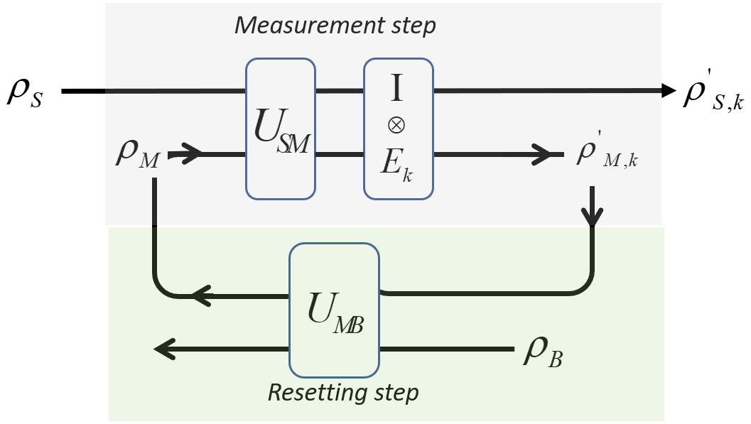
Figure 1: (Color online) Measurement scheme: A state $\rho_{S}$ is coupled to a memory register via unitary $U_{SM}$, followed by biased-unsharp POVM elements $E_{k}$ on the memory register. The memory is reset to its initial state $\rho_{M}$ using a thermal resource $\rho_{B}$, before the device is used again.

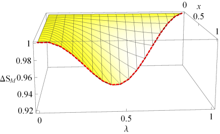
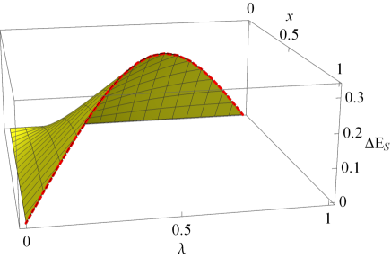
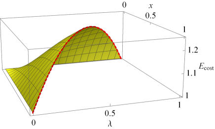
Figure 2: (Color online) Depicting the contributions to the energy cost $E_{cost}$ as defined in Eq. (17) with respect to bias ($x$) and sharpness ($\lambda$) (dimensionless) parameters, such that $x+\lambda\leq 1$, with the red (dashed) curve pertaining to equality.

The register $M$ in the measurement step stores a measurement outcome $k$ in a state $\rho_{M,k}^{\prime}\in\mathcal{S}(H_{M})$. In order to read out the measurement outcome from the register, one would apply the projectors $\{\Pi_{k}\}_{k}$ satisfying $\sum_{k}\Pi_{k}=\mathbb{1}$, on the respective subspaces $H_{k}$. Accordingly, the implementation of a quantum measurement is described by a tuple $(\rho_{M},U_{SM},\{\Pi_{k}\})$ where $\rho_{M}$ and $U_{SM}$ denote the initial state of the register and the unitary operator describing the interaction between system $S$ and register $M$. Therefore, one can think of the measurement process as a channel which maps an input state $\rho_{S}$ to an output state

$$\rho_{SM,k}^{\prime}=(\mathbb{1}\otimes\Pi_{k})U_{SM}(\rho_{S}\otimes\rho_{M})U_{SM}^{\dagger}(\mathbb{1}\otimes\Pi_{k})/p_{k}.$$ (16)

with probability $p_{k}=\operatorname{Tr}\big{[}(\mathbb{1}\otimes\Pi_{k})U_{SM}(\rho_{S}\otimes\rho_{M})U_{SM}^{\dagger}\big{]}$, such that $\rho_{SM}^{\prime}=\sum_{k}p_{k}~{}\rho_{SM,k}^{\prime}$, and the corresponding reduces states of the system and the memory register are respectively given by $\rho_{S}^{\prime}=\operatorname{Tr}_{M}[\rho_{SM}^{\prime}]$ and $\rho_{M}^{\prime}=\operatorname{Tr}_{S}[\rho_{SM}^{\prime}]$.

The total energy cost for measurement and resetting step turns out to be Abdelkhalek et al. (2016)

$$E_{cost}=\Delta E_{S}+\frac{1}{\beta}\Delta S_{M},$$ (17)

with $\Delta E_{S}=\operatorname{Tr}[H_{S}(\rho_{S}^{\prime}-\rho_{S})]$ and $\Delta S_{M}=S(\rho_{M}^{\prime})-S(\rho_{M})$. Thus the total energy cost is essentially determined by the entropy change in the memory. In what follows, we bring out the effect of biased-unsharp measurements on this quantity. Such measurements, often called inefficient measurements are characterized by Kraus operators $\{E_{i}\}$, such that the post-measurement state is given by $\rho^{\prime}=\sum_{i}E_{i}\rho E_{i}^{\dagger}$, with $1\leq i\leq r$, where $r$ is the Kraus rank, and $r=1$ corresponds to efficient measurements. Rewriting Eq. (1) as

$$E_{\pm}=\frac{1-\lambda\pm x}{2}\mathbb{1}+\lambda\Pi^{\pm}.$$ (18)

Here, $\lambda=|\vec{m}|$ is the sharpness parameter and $\Pi^{\pm}=(1\pm\hat{Q})/2$ are the sharp projectors corresponding to observable $\hat{Q}=\hat{m}.\vec{\sigma}$, assumed to be of the form given in Eq. (8). We take a simple model with of the system prepared in state $\rho_{S}=\frac{1}{2}|0\rangle\langle 0|+\frac{1}{2}|1\rangle\langle 1|$, a statistical mixture of the eigenstates of Hamiltonian $H_{S}=\omega_{S}\sigma_{z}$. Further, the memory is assumed to be in a two qubit state $\rho_{M}=|0\rangle\langle 0|_{M_{A}}\otimes\frac{1}{2}\mathbb{1}_{M_{B}}$. With the projectors $P_{k}=|k\rangle\langle k|\otimes\frac{1}{2}\mathbb{1}_{M_{B}}$, $k=0,1$ and the unitary interaction between the system and memory of the form Abdelkhalek et al. (2016)

$$U_{SM} =\Big{(}|0\rangle\langle 0|_{S}\otimes\mathbb{1}_{M_{A}}+|1\rangle\langle 1|_{S}\otimes\sigma^{x}_{M_{A}}\Big{)}\otimes\mathbb{1}_{M_{B}},$$ (19)

one can show that the measurement device represented by [$U_{SM},\rho_{M},\{P_{k}\}$] outputs the correct state $\rho_{M,k}^{\prime}=|k\rangle\langle k|_{M_{A}}\otimes\mathbb{1}_{M_{B}}$. However, we are interested in the situation when $\{P_{k}\}$ are not ideal projective measurements but are biased and have some unsharp. This is incorporated in the above scheme by replacing $|k\rangle\langle k|$ by $E_{k}$ given in Eq. (18), such that $\{P_{k}\}\rightarrow\{\tilde{P}_{k}\}=\{E_{k}\otimes\frac{1}{2}\mathbb{1}_{M_{B}}\}$, we have

$$\rho_{SM}^{\prime} =\sum_{k=\pm}(\mathbb{1}\otimes\tilde{P}_{k})U_{SM}(\rho_{S}\otimes\rho_{M})U_{SM}^{\dagger}(\mathbb{1}\otimes\tilde{P}_{k}).$$ (20)

The normalized reduced states of the system and memory are respectively given by

$$\rho_{S}^{\prime} =\frac{1}{2}\begin{pmatrix}1+R_{c}&0\\ 0&1-R_{c}\end{pmatrix},$$ (21)

$$\rho_{M}^{\prime} =\begin{pmatrix}\frac{1}{4}+\frac{1}{2}R_{c}&0&\frac{1}{2}R_{s}&0\\ 0&\frac{1}{4}+\frac{1}{2}R_{c}&0&\frac{1}{2}R_{s}\\ \frac{1}{2}R_{s}^{*}&0&\frac{1}{4}-\frac{1}{2}R_{c}&0\\ 0&\frac{1}{2}R_{s}^{*}&0&\frac{1}{4}-\frac{1}{2}R_{c}\end{pmatrix}.$$ (22)

Here $R_{c}=\frac{x\lambda}{1+x^{2}+\lambda^{2}}\cos(\Theta)$, $R_{s}=\frac{x\lambda}{1+x^{2}+\lambda^{2}}e^{i\Phi}\sin(\Theta)$ are introduced for convenience, and $\Theta$ and $\Phi$ are the measurement parameters defined in Eq. (8). It follows that with either $x=0$ or $\lambda=0$, both system as well as memory are found to be in maximally mixed state. The energy cost is proportional to the entropy change $\Delta S_{M}=S(\rho_{M}^{\prime})-S(\rho_{M})$ in the memory

$$\Delta S_{M} =-\sum\limits_{n=1}^{4}\eta_{n}\log_{2}(\eta_{n})-1,$$ (23)

where $\eta_{n}$ are the eigenvalues of $\rho_{M}^{\prime}$, with $\eta_{1}=\eta_{2}=\frac{1}{4}(1+\frac{2x\lambda}{1+x^{2}+\lambda^{2}}),\eta_{3}=\eta_{4}=\frac{1}{4}(1-\frac{2x\lambda}{1+x^{2}+\lambda^{2}})$, independent of the measurement parameters $\Theta$ and $\Phi$. This quantity is depicted in Fig. (2) with respect to bias and sharpness parameters. A decrease in $\Delta S_{M}$ is observed for non-zero values of these parameters, and is found to be minimum for $x=\lambda=1/2$. Further, the contribution to energy cost due to change in the system state is given by

$$\Delta E_{S} =\operatorname{Tr}\big{[}H_{S}(\rho_{S}^{\prime}-\rho_{S})\big{]}=\frac{2x\lambda\omega_{S}}{1+x^{2}+\lambda^{2}}\cos(\Theta).$$ (24)

In this particular example, the measurement on the system is performed in $\{\ket{0},\ket{1}\}$ basis, so we set $\Theta=\Phi=0$, which amount to $\mathcal{Q}=\sigma_{z}$ in Eq. (8). With this setting. $\Delta E_{S}$ is depicted in Fig. (2) for $\omega_{S}=1$, and attains maximum value for $x=\lambda=1/2$. The total energy cost $E_{cost}$ is positive and is also maximum for the measurement characterized by equal bias and sharpness. One can map this scenario with the non-Markovian amplitude damping channel for which the bias and sharpness are respectively given by $x=|G^{2}(t)-1|$ and $\lambda=|G(t)|^{2}$, for $\Theta=0$, see Table (1), where $G(t)$ is the memory kernel with following form Bylicka et al. (2014)

$$G(\uptau)=e^{-\uptau/2}\Bigg{[}\cosh(\sqrt{1-2R}~{}\uptau/2)+\frac{\sinh(\sqrt{1-2R}~{}\uptau/2)}{\sqrt{1-2R}}\Bigg{]}.$$ (25)

Here, $R$ is proportional to the coupling strength and $\uptau$, is dimensionless time. The regimes $2R\leq 1$ and $2R>1$ correspond to Markovian and non-Markovian dynamics, respectively. The time behavior of the memory kenel is depicted in Fig. (3), and is found to acquire negative values under non-Markovian dynamics. As time increases, $G(\uptau)\rightarrow 0$, and an arbitrary state subjected to AD channel settles to the ground state $\ket{0}$. Correspondingly the bias ($x$) and sharpness ($\lambda$) parameters tends to $1$ and $0$, respectively, and the POVM elements in Eq. (18) become $\{E_{+}=\mathbb{1},E_{-}=0\}$. Therefore, the fact that system is eventually found in ground state is equivalent to the statement that the POVM reduces to the identity operation. Notice that $G(\uptau)$ damps quickly as the coupling strength is increased. Therefore, the sharpness of our POVM decreases rapidly with increase in the degree of non-Markovianity of the noisy channel. This fact is reflected in the energy cost of performing such measurements, as depicted in Fig. (3).

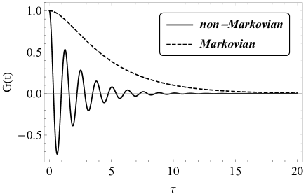
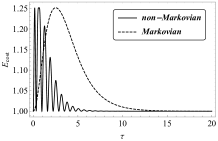
Figure 3: The memorial kernel $G(\uptau)$ (top) and energy cost $E_{cost}$ (bottom) as a function of dimensionless time parameter $\tau$.

IV Conclusion

Generalized dichotomic measurements characterized by bias and sharpness provide a way to take into account the different causes which make a measurement non-ideal. The bias quantifies tendency of a measurement to favor one state over the other while as sharpness is proportional to the precision of the measurement. In this work, we have shown how the bias and sharpness change under the action of a dynamical process (e.g. quantum channels) from the perspective of the Heisenberg picture. Specifically, we considered various quantum channels, both Markovian and non-Markovian. We have shown the unital channel induce unbiased measurements on a qubit state. Also, the conjugate of a unital channel acting on a projective measurement generates an unbiased POVM. Further, Markovian channels are shown to lead to measurements for which sharpness is a monotonically decreasing function of time. Hence, for unital channels, this provides a witness for P-indivisible form of non-Markovian dynamics.

Measurement process is central in carrying out operations with quantum devices in a controlled manner. With increasing complexity of quantum devices, the energy supply for carrying out the elementary quantum operations must be taken into account. We investigated the effect of bias and sharpness parameters on the energy cost of the measurement. The energy cost is proportional to the entropy of memory register which is found to decrease in presence of biased-unsharp measurements, however the total energy cost is found to increase under such measurements.

The present work may be extended to higher dimensional systems and by considering other definitions of non-Markovianity– via CP-divisibility of channels.

References

- Busch et al. (1996) P. Busch, P. J. Lahti, and P. Mittelstaedt, The quantum theory of measurement (Springer, 1996).
- Braginsky et al. (1992) V. B. Braginsky, F. Y. Khalili, and K. S. Thorne, Quantum Measurement (Cambridge University Press, 1992).
- Busch and Schmidt (2010) P. Busch and H.-J. Schmidt, Quantum Inf Process 9, 143 (2010).
- Yu et al. (2010) S. Yu, N.-l. Liu, L. Li, and C. H. Oh, Phys. Rev. A 81, 062116 (2010).
- Busch and Jaeger (2010) P. Busch and G. Jaeger, Found. Phys. 40, 1341 (2010).
- Das et al. (2018) D. Das, S. Mal, and D. Home, Phys. Lett. A 382, 1085 (2018).
- Acín et al. (2016) A. Acín, S. Pironio, T. Vértesi, and P. Wittek, Phys. Rev. A 93, 040102 (2016).
- Stano et al. (2008) P. Stano, D. Reitzner, and T. Heinosaari, Phys. Rev. A 78, 012315 (2008).
- Kumari and Pan (2017) S. Kumari and A. K. Pan, Phys. Rev. A 96, 042107 (2017).
- Sayrin et al. (2011) C. Sayrin, I. Dotsenko, X. Zhou, B. Peaudecerf, T. Rybarczyk, S. Gleyzes, P. Rouchon, M. Mirrahimi, H. Amini, M. Brune, et al., Nature 477, 73 (2011).
- Pal and Ghosh (2011) R. Pal and S. Ghosh, J. Phys. A: Math. Theor. 44, 485303 (2011).
- Li et al. (2019) Z. Li, H. Zhang, and H. Zhu, Phys. Rev. A 99, 062342 (2019).
- Watrous (2018) J. Watrous, The theory of quantum information (Cambridge University Press, 2018).
- Ruskai et al. (2002) M. B. Ruskai, S. Szarek, and E. Werner, Lin. Alg. Appl. 347, 159 (2002).
- Banerjee and Ghosh (2007) S. Banerjee and R. Ghosh, J Phys. A: Mathematical and Theoretical 40, 13735 (2007).
- Omkar et al. (2013) S. Omkar, R. Srikanth, and S. Banerjee, Quantum Inf Process 12, 3725 (2013).
- Banerjee (2018) S. Banerjee, Open Quantum Systems: Dynamics of Nonclassical Evolution, Vol. 20 (Springer, 2018).
- Srikanth and Banerjee (2008) R. Srikanth and S. Banerjee, Phys. Rev. A 77, 012318 (2008).
- Banerjee and Srikanth (2008) S. Banerjee and R. Srikanth, Eur. Phys. J. D 46, 335 (2008).
- Mendl and Wolf (2009) C. B. Mendl and M. M. Wolf, Commun. Math. Phys. 289, 1057 (2009).
- Daffer et al. (2004) S. Daffer, K. Wódkiewicz, J. D. Cresser, and J. K. McIver, Phys. Rev. A 70, 010304 (2004).
- Nielsen and Chuang (2002) M. A. Nielsen and I. Chuang, “Quantum computation and quantum information,” (2002).
- Bylicka et al. (2014) B. Bylicka, D. Chruściński, and S. Maniscalco, Sc. Rep. 4, 5720 (2014).
- Naikoo et al. (2019) J. Naikoo, S. Dutta, and S. Banerjee, Phys. Rev. A 99, 042128 (2019).
- Kumar et al. (2018) N. P. Kumar, S. Banerjee, R. Srikanth, V. Jagadish, and F. Petruccione, Open Systems & Information Dynamics 25, 1850014 (2018).
- Shrikant et al. (2020) U. Shrikant, R. Srikanth, and S. Banerjee, Sci. Rep. 20 (2020).
- Murnaghan (1962) F. D. Murnaghan, The unitary and rotation groups, Vol. 3 (Spartan books, 1962).
- Breuer et al. (2016) H.-P. Breuer, E.-M. Laine, J. Piilo, and B. Vacchini, Rev. Mod. Phys. 88, 021002 (2016).
- Abdelkhalek et al. (2016) K. Abdelkhalek, Y. Nakata, and D. Reeb, arXiv:1609.06981 (2016).
- Srikanth and Banerjee (2007) R. Srikanth and S. Banerjee, Phys. Lett. A 367, 295 (2007).