A Little Energy Goes a Long Way: Build an Energy-Efficient, Accurate Spiking Neural Network from Convolutional Neural Network

Abstract

This paper conforms to a recent trend of developing an energy-efficient Spiking Neural Network (SNN), which takes advantage of the sophisticated training regime of Convolutional Neural Network (CNN) and converts a well-trained CNN to an SNN. We observe that the existing CNN-to-SNN conversion algorithms may keep a certain amount of residual current in the spiking neurons in SNN, and the residual current may cause significant accuracy loss when inference time is short. To deal with this, we propose a unified framework to equalise the output of convolutional or dense layer in CNN and the accumulated current in SNN, and maximally align spiking rate of a neuron with its corresponding charge. This framework enables us to design a novel explicit current control (ECC) method for the CNN-to-SNN conversion which considers multiple objectives at the same time during the conversion, including accuracy, latency and energy efficiency. We conduct an extensive set of experiments on different neural network architectures, e.g. VGG, ResNet and DenseNet, to evaluate the resulting SNNs. The benchmark datasets include not only the image datasets such as CIFAR-10/100 and ImageNet but also the Dynamic Vision Sensor (DVS) image datasets such as DVS-CIFAR-10. The experimental results show the superior performance of our ECC method over the state-of-the-art.

1 Introduction

Spiking neural networks (SNNs) are more energy efficient than convolutional neural networks (CNNs) in inference time thanks to its utilisation of matrix addition instead of multiplication. SNNs are supported by new computing paradigms and hardware. For example, SpiNNaker [21], a neuromorphic computing platform based on SNNs, can run real-time billions of neurons to simulate human brain. The neuromorphic chips, such as TrueNorth [1], Loihi [3], and Tianji [23], can directly implement SNNs with 10,000 neurons being integrated onto a single chip. Moreover, through the combination with sensors, SNNs can be applied to edge computing, robotics, and other fields, to build low-power intelligent systems [24].

However, the discrete nature of spikes makes the training of SNNs hard, due to the absence of gradients.

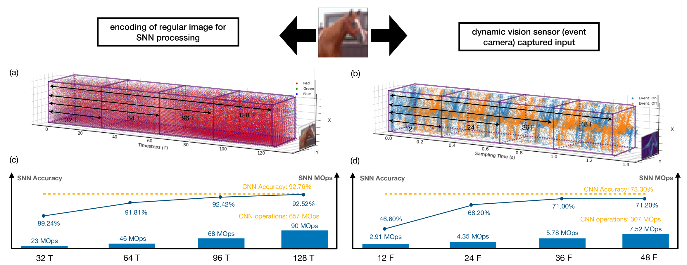
Figure 1: An illustrative diagram showing how SNNs process two different types of inputs and their performance comparison with CNNs. A regular image (left column) – taken from camera – is preprocessed into a spike train (A), which then runs through the SNN in a number of timesteps (e.g., 128 timesteps as in the figure). A DVS input – taken from event camera – can be represented directly as a spike train (B), and processed naturally by the SNN in a number of frames (e.g., 48 frames as in the figure). (C) and (D) show the SNN’s performance with respect to the three objectives (accuracy, energy efficiency, and latency), comparing to CNNs.

This paper follows a cutting-edge approach of obtaining a well-performed SNN by converting from a trained CNN of the same structure. This approach has an obvious benefit from the sophisticated training regime of CNNs, i.e., it is able to take advantage of the successful – and still fast improving – training methods on CNNs without extra efforts to adapt them to SNNs. Unfortunately, existing CNN-to-SNN conversion methods either cannot achieve a sufficiently small accuracy loss upon conversion [27, 31], or need a high latency [31], or require a significant increase on the energy consumption of the resulting SNNs [6]. Moreover, recent methods such as [6] do not work with batch-normalisation layer – a functional layer that plays a key role in the training of CNNs [29].

This paper levels up the CNN-to-SNN conversion with the following contributions. First of all, methodologically, we argue that, the conversion needs to be multi-objective – in addition to accuracy loss, energy efficiency and latency should be considered altogether. Figure 1 provides an illustration showing how SNNs process images and DVS inputs, exhibiting how well our methods enable the achievement of the three objectives and its comparison with CNNs. Actually, from (C) and (D) of Figure 1, SNNs can have competitive accuracy upon conversion (92.52% vs 92.76%, and 71.20% vs 73.30%, respectively) and be significantly more energy efficient than CNNs (90MOps vs 657MOps, and 7.52MOps vs 307MOps, respectively). While it is hard to compare the latency as SNNs and CNNs work on different settings, our method implements the high energy efficiency with low latency (128 timesteps for images and 48 frames for DVS inputs). As shown in our experiments, ours are superior to the state-of-the-art conversions [27, 31, 6].

Second, we follow an intuitive view aiming to establish an equivalence between the activations in an original CNN and the current in the resulting SNN. This view inspires us to consider an explicit, and detailed, control on the current flowing through the SNN. Technically, we develop a unifying theoretical framework, which treats both weight normalisation [27] and threshold balancing [31] as special cases. Based on the framework, we develop a novel conversion method called explicit current control (ECC), which includes two techniques: current normalisation (CN), to control the maximum number of spikes fed into the SNN, and thresholding for residual elimination (TRE), to reduce the residual membranes potential in the neurons.

Third, we include in ECC a dedicated technique called consistency maintenance for batch-normalisation (CMB) to deal with the conversion of batch-normalisation layer.

Finally, we implement ECC into a tool SpKeras and conduct an extensive set of experiments on not only the regular image datasets, such as CIFAR-10/100 and ImageNet, but also the Dynamic Vision Sensor (DVS) datasets such as DVS-CIFAR-10. Note that, DVS datasets are dedicated for SNN processing. The experimental results show that, comparing with state-of-the-art methods [27, 31, 6], ECC can optimise over three objectives at the same time, and have superior performance. Moreover, we notice that (1) ECC can utilise the conversion of batch-normalisation to reduce the latency, and (2) ECC is robust to the hardware deployment because the quantisation – by using 7-10 bits to represent the originally 32-bit weights – does not lead to significant accuracy loss.

We remark that, this paper is not to argue for the replacement of CNNs with SNNs in general. Instead, we suggest a plausible deployment workflow, i.e., train a CNN $\rightarrow$ convert into an SNN $\rightarrow$ deploy on edge devices with e.g., event camera. The workflow will not be a good option if any of the three objectives is not optimised.

2 Related Work

2.1 Current “energy for accuracy” trend in CNN-to-SNN Conversion

A few different conversion methods, such as [5, 27, 31, 6], have been proposed in the past few years. It is not surprising that there is an accuracy loss between SNNs and CNNs. For example, in [27, 31], the gap is between 0.15% - 2% for CIFAR10 networks. A recent work [31] shows that this gap can be reduced if we use a sufficiently long (e.g., 1024 timesteps) spike train to encode an input. However, a longer spike train will inevitably lead to higher latency. This situation was believed to be eased in [6], which claims that the length of spike train can be drastically shortened in order to achieve near-zero accuracy loss. However, as shown in Section 4.2 (Figure 3A), their threshold scaling method can easily lead to a significant increase on the spike-caused synaptic operations [27], or spike operations for short, which also lead to significant increase on the energy consumption.

Other related works include [26, 25, 17], which calibrate SNN to a specific timestep by gradient-based optimisation. The calibration requires extra training time to find the optimal weights or hyper-parameters, such as some thresholds. In contrast, [4] trained a dedicated CNN for an SNN with fixed timesteps by shifting and clipping ReLU activations, although the accuracy loss of these SNNs cannot converge to zero when increasing the timesteps, as shown in Figure 6B. Besides, instead of reducing spikes, [19] explored SNN with binary weights to further improve the energy efficiency by consuming less memory.

2.2 Technical Ingredients in CNN-to-SNN Conversion

	HR	SR	WN∗	TB∗	TS	ECC	BN∗∗	MP	AP
[2]	$\surd$								$\surd$
[5]	$\surd$		$\surd$						$\surd$
[27]		$\surd$	$\surd$				$\surd$	$\surd$
[31]	$\surd$			$\surd$					$\surd$
[6]		$\surd$		$\surd$	$\surd$				$\surd$
[this paper]		$\surd$	$\surd$	$\surd$		$\surd$	$\surd$		$\surd$

Table 1: Comparison of Key Technical Ingredients (HR, SR, WN, TB, TS, ECC) and Workable Layers (BN, MP, AP) with the State-of-the-Art Methods. HR: hard reset; SR: reset by subtraction, or soft reset; WN: weight normalisation; TB: threshold balancing; TS: threshold scaling; ECC: explicit current control; BN: batch normalisation; MP: max pooling; AP: average pooling. * As a contribution of this paper, in Section 3.2, we show that both WN and TB are special cases of our ECC framework. ** Among all methods, only those that can handle BN have bias terms in their pre-trained CNNs.

Table 1 provides an overview of the existing conversion methods [2, 5, 27, 31, 6] and ours, from the aspects of technical ingredients and workable layers. At the beginning, most of the techniques, such as [2, 5], are based on hard reset (HR) spiking neurons, which are reset to fixed reset potential once its membrane potential exceeds the firing threshold. HR is still used in some recent methods such as [31]. The main criticism on HR is its significant information loss during the SNN inference. Soft reset (SR) neurons are shown better in other works such as [27, 6].

Weight normalisation (WN) is proposed in [5] and extended in [27] to regulate the spiking rate in order to reduce accuracy loss. The other technique, threshold balancing (TB), is proposed in [31] and extended in [6], to assign appropriate threshold to the spiking neurons to ensure that they operate in the linear (or almost linear) regime. We show in Section 3.2 that both WN and TB are special cases of our theoretical framework.

Another technique, called threshold scaling (TS), is suggested in [6]. However, as our experimental result shown in Figure 3A, TS leads to a significantly greater energy consumption (measured as MOps). On the other hand, our ECC method can achieve smaller accuracy loss and significantly less energy consumption.

We also note in Table 1 the differences in terms of workable layers in CNNs/SNNs for different methods. For example, batch-normalisation (BN) layer [7] is known important for the optimisation of CNNs [29], but only one existing method, i.e., [27], can work with it. Similarly for the bias values of neurons which are pervasive for CNNs. Actually, the consideration of BN is argued in [31] as the key reason for the higher accuracy loss in [27]. The results of this paper show that, we can keep both BN and bias without significant increased energy consumption, by maintaining the consistency between the behaviour of SNN and CNN. BN can help with the reduction of latency. As we discussed earlier and in Section 5, our ECC method may be applicable to B-SNN and further improve its performance. Moreover, we follow most SNN research to consider average pooling (AP) layer instead of max pooing (MP) layer.

2.3 Direct Training

SNNs process information through non-differentiable spikes, and thus the backpropagation (BP) [13] training algorithm cannot be directly applied. A few attempts [15, 14] have been made to adapt the BP algorithm by approximating its forward propagation phase. Such direct training requires high computational complexity to achieve an accuracy that is close to CNNs [35]. Unlike these methods which approximate the BP algorithm [15, 14], both of which may lead to performance degradation, we choose CNN-to-SNN conversion which can take full advantage of the continuously improving CNN training methods. Other than these methods which try to re-produce the success of CNN training, there are other direct training methods, such as approaches based on reservoir computing ([33]) and evolutionary algorithms ([30]).

3 Explicit Current Control (ECC)

By leveraging the correspondence between activation in CNNs and current in SNNs, we propose a unifying theoretical framework targeting multiple objectives, including accuracy, latency and energy efficiency. Going beyond the existing conversion techniques (see Table 1) that consider some of the objectives individually, we view these multi-objective holistically through the lens of the unifying theoretical framework. Inspired by such new viewpoint, we develop explicit current control (ECC) techniques to normalise, clip, and maintain the current through the SNNs for the purposes of reducing accuracy loss, latency, and energy consumption.

3.1 Existing CNN-to-SNN Conversion

Without loss of generality, we consider a CNN model of $N$ layers such that layer $n$ has $M^{n}$ neurons, for $n\in\{1,2,\dots,N\}$. The output of the neuron $i\in\{1,\dots,M^{n}\}$ at layer $n$ with ReLU activation function is given by

$$a_{i}^{n}=\max\left\{0,\sum_{j=1}^{M^{n-1}}W_{ij}^{n}a_{j}^{n-1}+b^{n}_{i}\right\}$$ (1)

where $W_{ij}^{n}$ is the weight between the neuron $j$ at layer $n-1$ and the neuron $i$ at layer $n$, $b_{i}^{n}$ is the bias of the neuron $i$ at layer $n$, and $a_{i}^{0}$ is initialised as the input $x_{i}$.

The activation $a_{i}^{n}$ indicates the contribution of the neuron to the CNN inference. For CNN-to-SNN conversion, the greater $a_{i}^{n}$ is, the higher spiking rate will be, for the corresponding neuron on SNN. An explanation of a conversion method from CNNs to SNNs was first introduced in [27] by using data-based weight normalisation.

The conversion method uses integrated-and-fire (IF) neuron to construct a rate-based SNN without leak and refractory time. If considering practical implementations, the rate-based SNN expects a relatively large interval between input spikes to minimise the effect of refractory time. To convert from a CNN, the spiking rate of each neuron in SNN is related to the activation of its corresponding neuron in the CNN. An iterative algorithm based on the reset by subtraction mechanism is described below. The membrane potential $V_{i}^{n}(t)$ of the neuron $i$ at the layer $n$ can be described as

$$V_{i}^{n}(t)=V_{i}^{n}(t-1)+Z_{i}^{n}(t)-\Theta_{i}^{n}(t)V^{n}_{thr}$$ (2)

where $V^{n}_{thr}$ represents the threshold value of layer $n$ and $Z^{n}_{i}(t)$ is the input current to neuron $i$ at layer $n$ such that

$$Z^{n}_{i}(t)=\sum_{j=1}^{M^{n-1}}W_{ij}^{n}\Theta_{j}^{n-1}(t)+b^{n}_{i}$$ (3)

with $\Theta_{i}^{n}(t)$ being a step function defined as

$$\Theta_{i}^{n}(t)=\left\{\begin{matrix}1,&\text{ if }V_{i}^{n}(t)\geq V_{thr}^{n}\\ 0,&\text{otherwise. }\end{matrix}\right.$$ (4)

In particular, when the current $V^{n}_{i}(t)$ reaches the threshold $V_{thr}^{n}$, the neuron $i$ at layer $n$ will generate a spike, indicated by the step function $\Theta_{i}^{n}(t)$, and the membrane potential $V_{i}^{n}(t)$ will be reset immediately for the next timestep by subtracting the threshold.

3.2 A Unifying Theoretical Framework

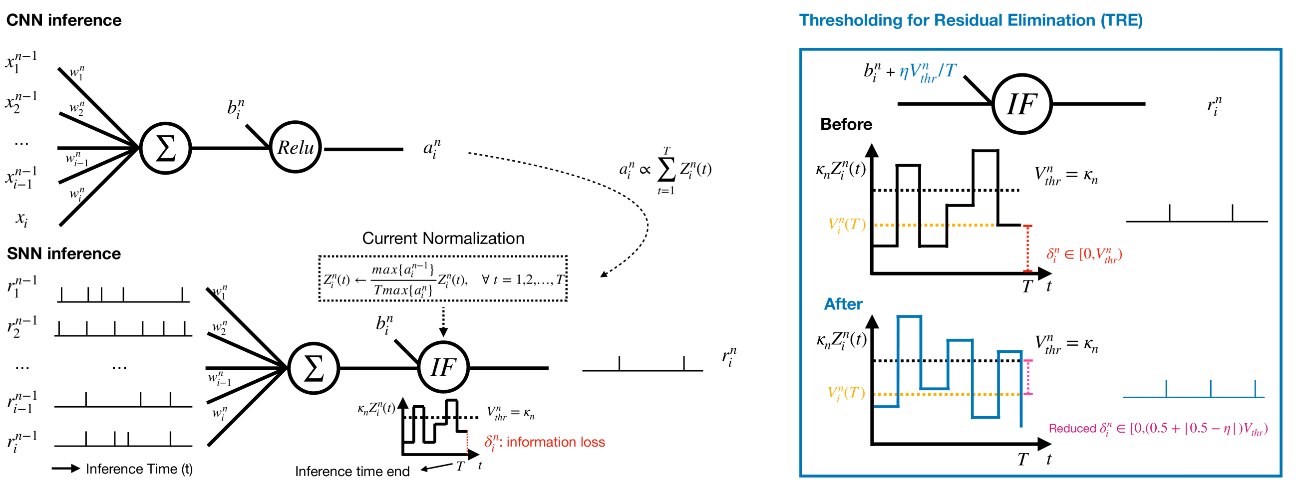
Figure 2: Left: Our proposed CNN-to-SNN conversion for the $n$-th layer with a current normalisation component and a thresholding mechanism. The activation $a_{i}^{n}$ in the CNN (Top) is used for current normalisation in the SNN (Bottom). Right: The proposed Thresholding for Residual Elimination (TRE) and the illustration of error reduction by TRE.

The above CNN-to-SNN conversion method is designed specifically for weight normalisation [27], and cannot accommodate other conversion methods, e.g., threshold balancing [31]. We propose a novel theoretical framework for CNN-to-SNN conversion that covers both weight normalisation [27] and threshold balancing [31] as special cases. In particular, the proposed framework improves over [27] by adopting a thresholding mechanism to quantify the accumulated current into spikes in SNN, and extends the threshold balancing mechanism to be compatible with batch normalisation and bias.

We will work with the spiking rate of each SNN neuron $i$ at layer $n$, defined as $r_{i}^{n}(t)=N_{i}^{n}(t)/t$, where $N_{i}^{n}(t)$ is the number of spikes generates in the first $t$ timesteps by neuron $i$ at layer $n$. We remark that, it is possible that $r_{i}^{n}(t)>1$, i.e., multiple spikes in a single timestpes, in which case the latency is increased to process extra spikes.

Our framework is underpinned by Proposition  1.

Proposition 1

In the CNN-to-SNN conversion, if the first layer CNN activation $a_{i}^{1}$ and the first layer SNN current $Z^{1}_{i}(t)$ satisfy the following condition

$$\frac{1}{T}\sum_{t=1}^{T}Z^{1}_{i}(t)=a_{i}^{1},$$ (5)

where $T$ is a predefined maximum timesteps, then the SNN spiking rate at time step $t$ can be iteratively computed by

$$\begin{array}[]{l}\displaystyle r^{n}_{i}(t)=\frac{1}{V^{n}_{thr}}\Big{(}\sum^{M^{n-1}}_{j=1}W^{n}_{ij}r_{j}^{n-1}(t)+b_{i}^{n}\Big{)}-\Delta_{i}^{n}(t)\end{array}$$ (6)

with $\Delta_{i}^{n}(t)\triangleq\displaystyle{V^{n}_{i}(t)}/{(tV^{n}_{thr})}$ representing the residual spiking rate. Initially, the spiking rate of neuron $i$ at the first layer is $r^{1}_{i}(t)=a^{1}_{i}/V^{1}_{thr}-\Delta_{i}^{1}(t)$.

Remark 1

The spiking rate in Equation (6) is a generalised form of those using weight normalisation (WN) [27] and threshold balancing (TB) [31]. When keeping $\displaystyle V^{1}_{thr}=1$, by normalising $W^{n}_{ij}$ we obtain WN; when keeping $W^{n}_{ij}$ unchanged, by normalising $V^{n}_{thr}$ we obtain TB. When applying a scaling factor $\alpha^{n}$ to the threshold $V^{n}_{thr}$, Proposition 1 recovers [6].

The condition in Equation (5) bridges between the activations in CNNs and the accumulated currents in SNNs, i.e., within the duration of a spike train, the average accumulated current equals to the CNN activation. This is key to our theoretical framework, and different from some previous conversion method such as [27], which bridges between activations and firing rates. This activation-current association is reasonable because it aligns with the intuitions that (i) given a fixed spiking rate, a greater CNN activation requires a greater accumulated current in the SNN; and (ii) given a pre-trained CNN, more input spikes lead to increased current in the SNN.

Proposition 1 suggests that an explicit, optimised control on the currents may bring benefits to the spiking rate (so as to reduce energy consumption) and the residual current (so as to reduce the accuracy loss) simultaneously. Firstly, a normalisation on the currents $Z_{i}^{n}(t)$ is able to control the spike number, with its details being given in Section 3.3.1. Secondly, the error term $\Delta_{i}^{n}(t)$ will accumulate in deeper layers, causing lower spiking rate in the output layer [27]. The thresholding technique in Section 3.3.2 will be able to reduce impact from such error. Thirdly, we need to maintain the consistency between CNN and SNN so that the above control can be effective, as in Section 3.3.3.

The input is encoded into spike train via Poisson event-generation process [31] or interpreting the input as constant currents [27]. In this paper we select the latter.

3.3 ECC-Based Conversion Techniques

We develop three ECC-based techniques, including current normalisation (CN), thesholding for residual elimination (TRE), and consistency maintenance for batch-normalisation (CMB). Figure 2 illustrates CN and TRE, where the $n$-th layer of CNN is on the top and the corresponding conversed SNN layer is at the bottom. In the converted SNN layer, the sequences of spikes from the previous layer are aggregated, from which the current $Z_{i}^{n}(t)$ is accumulated in the neurons, and normalised by a factor (see Equation (7) below) to ensure that the increase of current at each timestep is within the range of $[0,1]$. The membrane potential $V_{i}^{n}(t)$ is produced according to Equation (2), followed by a spike generating operation as in Equation (4) once $V_{i}^{n}(t)$ exceeds the threshold $V_{thr}^{n}=\kappa_{n}$. The parameter $\kappa_{n}$ is the current amplification factor, which will be explained in Section 3.3.1. The residual current $\Delta_{i}^{n}$ at the end of spike train indicates the information loss in SNNs.

3.3.1 Current Normalisation (CN)

At layer $n$, before spike generation, CN normalises the current $Z^{n}_{i}(t)$ by letting

$$Z^{n}_{i}(t)\leftarrow\frac{\lambda_{n-1}}{T\lambda_{n}}Z^{n}_{i}(t),\quad\forall\;t=1,\dots,T$$ (7)

where $\lambda_{n}\triangleq\max_{i}\{a_{i}^{n}\}$ for $n=1,2,\dots,N$. We have $\lambda_{0}=1$ when the input has been normalised into $[0,1]$ for every feature. The benefit of CN is two-fold:

• By CN, the maximum number of spikes fed into the SNN is under control, i.e., we can have a direct control on the energy consumption.

• It facilitates the use of a positive integer $V_{thr}^{n}=\kappa_{n}$ as the threshold to quantify the current, which is amplified by factor of $\kappa_{n}$, for spike generation. In doing so, the neuron with maximum current can generate spike at every time step.

We randomly choose $\kappa_{n}=100$ for $V_{thr}^{n}$ and normalise weights for all experiments, except quantised SNN. Since the scalar of quantized weights in each layer will be absorbed into the threshold, we will get a different threshold for each layer. The quantisation process is explained in Section 4.4.

To achieve CN, the following conversion can be implemented to normalise weights and bias as follows.

$$W^{n}_{ij}\leftarrow\kappa_{n}\frac{\lambda_{n-1}}{\lambda_{n}}W^{n}_{ij},~{}b^{n}_{i}\leftarrow\frac{\kappa_{n}b^{n}_{i}}{\lambda_{n}},~{}V^{n}_{thr}\leftarrow\kappa_{n}.$$ (8)

Note that, the next layer will amplify the incoming current back to its original scale before its normalisation. When $\kappa_{n}=1~{}or~{}\lambda_{n}/\lambda_{n-1}$, the conversions correspond to weight normalisation in [27] and threshold balancing in [31] respectively.

3.3.2 Thresholding for Residual Elimination (TRE)

According to Equation (6), the error increment after conversion is mainly caused by the residual information, $\delta_{i}^{n}(T)\in[0,V^{n}_{thr}]$, which remains with each neuron after $T$ timesteps and cannot be forwarded to higher layers. To mitigate such errors, we propose a technique TRE to keep $\delta_{i}^{n}(T)$ under a certain value (half of $V_{thr}^{n}$ as in our experiments). In particular, we add extra current to each neuron in order to have $\eta V_{thr}^{n}$ increment on each membrane potential, where $\eta\in[0,1)$. Specifically, we update the bias term $b_{i}^{n}$ of neuron $i$ at layer $n$ as follows

$$b_{i}^{n}(t):=b_{i}^{n}(t)+\eta V^{n}_{thr}/T$$ (9)

for every timestep $t$. Intuitively, we slightly increase synaptic bias for every neuron at every step, so that a small volume of current is pumped into the system continuously.

The following proposition says that this TRE technique will be able to achieve a reduction of error range, which directly lead to the improvement to the accuracy loss.

Proposition 2

Applying TRE will lead to

$$\Theta_{i}^{n}(T)=\left\{\begin{matrix}1,&\text{if $V_{i}^{n}(T)>(1-\eta)V^{n}_{thr}$}\\ 0,&\text{otherwise.\hskip 56.9055pt}\end{matrix}\right.$$ (10)

for timestep $T$, as opposed to Equation (4). By achieving this, the possible range of errors is reduced from $[0,V^{n}_{thr})$ to $[0,(0.5+|0.5-\eta|)V^{n}_{thr})$.

We remark that, deploying TRE will increase at most one spike per neuron at the first layer and continue to affect the spiking rate at higher layers. This is the reason why we have slightly more spike operations than [27], as shown in Figure S1C in SM. A typical value of $\eta$ is 0.5.

3.3.3 Consistency Maintenance for Batchnormalisation (CMB)

Batch normalisation (BN) [7] accelerates the convergence of CNN training and improves the generalisation performance. The role of BN is to normalise output of its previous layer, which allows us to add the normalised information to weights and bias in the previous layer. We consider a conversion technique CMB to maintain the consistency between SNN and CNN in operating BN layer, by requiring a constant for numerical stability $\epsilon$, as follows.

$$\hat{W}^{n}_{ij}=\frac{\gamma_{i}^{n}}{\sqrt{\sigma_{i}^{n2}+\epsilon}}W^{n}_{ij}$$ (11)

$$\hat{b}^{n}_{i}=\frac{\gamma_{i}^{n}}{\sqrt{\sigma_{i}^{n2}+\epsilon}}(b^{n}_{i}-\mu_{i}^{n})+\beta_{i}^{n}$$ (12)

where $\gamma_{i}^{n}$ and $\beta_{i}^{n}$ are two learned parameters, $\mu_{i}^{n}$ and $\sigma_{i}^{n}$ are mean and variance. $\epsilon$ is platform dependent: for Tensorflow it is default as 0.001 and for PyTorch it is 0.00001. The conversion method in [27] does not consider $\epsilon$, and we found through a number of experiments that a certain amount of accuracy loss can be observed consistently. Figure 5 shows the capability of CMB in reducing the accuracy loss.

4 Experiment

We implement the ECC method and conduct an extensive set of experiments to validate it. We consider its comparison with the state-of-the-art CNN-to-SNN conversion methods on images and DVS inputs (Section 4.2 and Section 4.5, respectively), the demonstration of its working with batch-normalisation (Section 4.3), its robustness with respect to hardware deployment (Section 4.4), and an ablation study (Section 4.6). Due to the space limit, we present a subset of the results – the Supplementary Material (SM) include more experimental results. We fix $\kappa_{n}=100$ and $\epsilon=0.001$ throughout the experiments.

In this section, ‘2017-SNN’ denotes the method proposed in [27]. ‘RMP-SNN(0.8)’ and ‘RMP-SNN(0.9)’ denote the method in [6], with different parameter 0.8 or 0.9 as co-efficient to $V_{thr}$. ‘ECC-SNN’ is the our method. We remark that, it is shown in [6] that its conversion method outperforms that of [31], so we only compare with [6]. Moreover, we may write ‘Method@$n$T’ to represent the specific ‘Method’ when considering the spike trains of length $n$. Note that, only the CNN model in Figure 3A was trained without bias and BN, in order to have a fair comparison with RMP-SNN techniques. Since BN layers play an important role in training a high performance CNN and has the benefit of lowering the latency (c.f. Section 4.3), we believe it is essential to include it in CNN training. Therefore, we do not compare with [6] (i.e., RMP-SNN) and [31] in other experiments because they do not work with BN.

Before proceeding, we explain how to estimate energy consumption. For CNNs, it is estimated through the multiply–accumulate (MAC) operations

$$\textit{MAC operations for CNNs}:\sum_{n=1}^{N}(2f^{n}_{in}+1)M^{n}$$ (13)

where $f^{n}_{in}$ is the number of input connections of the $n$-th layer. The number of MAC operations are fixed when the architecture of the network is determined. For SNNs, the synaptic operations are counted to estimate the energy consumption of SNNs [20, 27], as follows.

$$\textit{Synaptic operations for SNNs}:\sum_{t=1}^{T}\sum_{n=1}^{N}f^{n}_{out}s^{n}$$ (14)

where $f^{n}_{out}$ is the number of output connections and $s^{n}$ is the average number of spikes per neuron, of the $n$-th layer.

4.1 Experimental Settings

We work with both image datasets (CIFAR-10/100 [11] and ImageNet [28]) and DVS datasets (CIFAR-10-DVS [16]) on several architectures [32] (VGG-16, VGG-19, and VGG-7). All the experiments are conducted on a CentOS Linux machine with two 2080Ti GPUs and 11 GB memory.

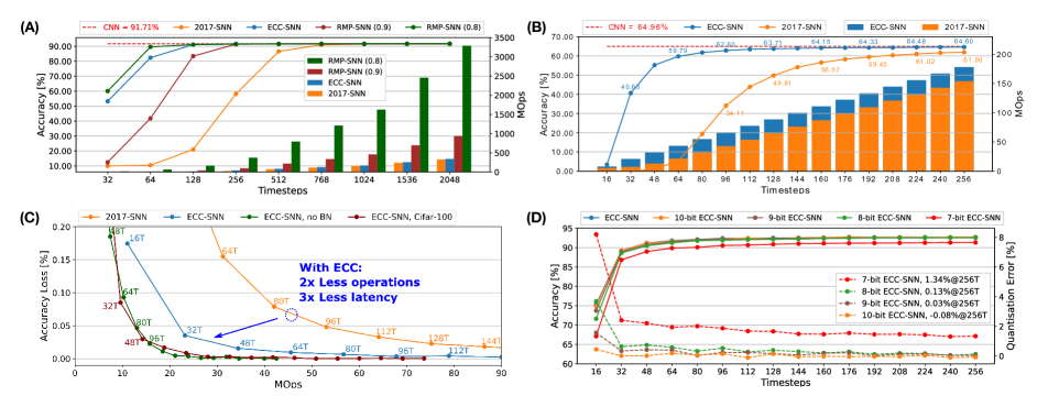
Figure 3: (A) Accuracy and energy consumption (MOps) w.r.t. timesteps for CIFAR-10. (B) Accuracy and energy consumption (MOps) w.r.t. timesteps, for ImageNet (Top-1 Acc). (C) Accuracy loss and latency w.r.t. energy consumption (MOps), for CIFAR-10 and CIFAR-100. (D) Accuracy and quantisation error w.r.t. timesteps, for CIFAR-10.

4.2 Comparisons with State-of-the-Art

Figure 3A presents a comparison between 2017-SNN, RMP-SNN, and ECC-SNN on both accuracy and energy consumption w.r.t. the timesteps, on VGG-16 and CIFAR-10. We note that, both RMP-SNN and ECC-SNN outperform 2017-SNN, in terms of the number of timesteps to reach near-zero accuracy loss. Furthermore, ECC-SNN is better than RMP-SNN(0.9) and competitive with RMP-SNN(0.8) in terms of reaching near-zero accuracy loss under certain latency. Specifically, both ECC-SNN and RMP-SNN(0.8) require 128 timesteps and RMP-SNN(0.9) requires 256 timesteps. Importantly, we note that, both RMP-SNN(0.8) and RMP-SNN(0.9) consume much more energy, measured with MOps, than ECC-SNN. Actually, ECC-SNN does not consume significantly more energy than 2017-SNN. Similar results can be extended to large dataset such as ImageNet. Moreover, to investigate further into the energy consumption, Figure 3B presents a comparison with 2017-SNN. All the above results show that ECC-SNN significantly reduces the latency, easily reaches the near-zero loss, and costs a minor increase on the energy.

The above results, together with those in SM (Figure S1A, Figure S1C, Figure S1D, and Figure S1E), reflect exactly the advantage of using ECC-SNN. That is, RMP-SNN(0.8) and ECC-SNN are the best in achieving near-zero accuracy loss with low latency, but RMP-SNN requires significantly more energy than the other two methods. Therefore, ECC-SNN achieves the best when considering energy, latency, and accuracy loss.

Batch-normalisation (BN) has become indispensable to train CNNs, so we believe a CNN-to-SNN method should be able to work with it. After demonstrating clear advantage over RMP-SNN, for the rest of this section, we will focus on the comparison with 2017-SNN, which deals with BN. We trained CNNs using Tensorflow by having a batch-normalisation layer after each convolutional layer.

4.3 Batch-normalisation (BN)

Figure 3C considers the impact of working with BN. Comparing with 2017-SNN, ECC-SNN achieves similar accuracy loss by taking 2x less MOps and 3x less latency. Moreover, to achieve the same accuracy loss, ECC-SNN without BN, i.e., ECC applies on CNNs without BN layers, requires significantly more timesteps, with slightly less MOps. Moreover, our other experiments show that, RMP-SNN (0.8), without BN in its method, can only achieve 48.32% in 256T. With BN, 2017-SNN can achieve 49.81% in 128T. ECC-SNN further improves on this, achieving 63.71% in 128T. That is, batch-normalisation under ECC-SNN can help reduce the latency. This is somewhat surprising, and we believe further research is needed to investigate the formal link between BN and latency.

4.4 Robustness to Quantisation

Figure 3D (and Figure S1B in SM) present how the change on the number of bits to represent weights may affect the accuracy and the quantisation error. This is an important issue, as the SNNs will be deployed on neuromorphic chip, such as Loihi [3] and TrueNorth [1], or FPGA, which may have different configurations. For example, Loihi can have weight precision at 1-9 bits. Floating-point data, both weights and threshold, can be simply converted into fixed-point data after CN in two steps: normalising the weights into range [-1,1] and scaling the threshold using the same normalisation factor, and then multiplied with $2^{b}$, where $b$ is the bit width [9, 34]. From Figure 3D and Figure S1B , the reduction from 32-bit to 10-, 9-, 8- and 7-bit signed weights does lead to drop on the accuracy, but unless it goes to 7-bit, the accuracy loss is negligible. This shows that, our ECC method is robust to hardware deployments.

4.5 DVS Dataset

CIFAR-10-DVS [16] is a benchmark dataset of DVS inputs, consisting of 10,000 inputs extracted from CIFAR-10 dataset using a DVS128 sensor. The resolution of data is 128x128. We preprocess the data following [35, 12], select the first 1.3s of the event stream, and down-scale the input into 42x42. For each dimension of an input, we calculate the number of spikes over the 1.3s simulation and normalise with a constant representing the maximum number of spikes. During SNN processing, as shown in Figure 1(B), the latency is based on the spikes. The experiments using VGG7 (Figure 5) , VGG16 and ResNet-18 [31] (Figure S2A and S2B in SM) show that ECC-SNN performs much better than 2017-SNN, who also work with BN layer. Moreover, in Table 2, we compare with a few methods including a recent direct training method. We can see that ECC-SNN can always achieve better accuracy, less frames, and less energy consumption.

Moreover, we recall the results shown in Figure 1 concerning the comparison between DVS inputs and images. For the same problem, if we choose the deployment workflow of “training a CNN $\rightarrow$ converting into an SNN $\rightarrow$ deploying on edge devices with e.g., event camera”, we may consume 10+ times less energy (7.52MOps vs 90MOps for CIFAR-10) by taking DVS inputs. Both are in stark contrast with the other deployment workflow “training a CNN $\rightarrow$ deploying on edge devices with camera”, which costs much more energy (307MOPs and 657MOps, respectively).

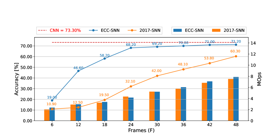
Figure 4: Accuracy and energy consumption (MOps) w.r.t. frames, between 2017-SNN and ECC-SNN, for CIFAR-10-DVS and VGG-7.

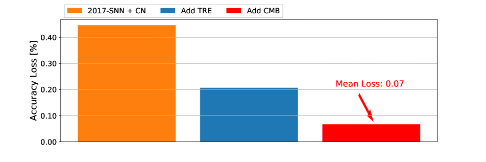
Figure 5: Contribution of CN, CMB, and TRE to the reduction of mean accuracy loss, for CIFAR-10 and VGG-16.

Method	Accuracy	N${}^{*}_{f}$	MOps
Direct training (VGG7) [35]	62.50	-	-
2017-SNN (DenseNet) [12]	65.61	60	1,551
ECC-SNN (VGG16)	71.20	48	66.79
ECC-SNN (VGG7)	71.30	48	7.52

*N_f is the number of frames.

Table 2: Comparison of SNN accuracy, latency and energy consumption (MOps), between direct training, 2017-SNN and ECC-SNN, for Cifar-10-DVS

4.6 Ablation Study

To understand the contributions of the three ingredients of ECC-SNN, i.e., CN, CMB, and TRE, we conduct an experiment on VGG-16 and CIFAR-10, by gradually including technical ingredients to see their respective impact on the accuracy loss. Figure 5 shows the histograms of the mean accuracy losses in 256T, over the 281-283th epochs. We see that, every ingredient plays a role in reducing the accuracy loss, with the TRE and CN being lightly Moreover, We also consider the impact of $\eta$ (as in Figure S1F of SM).

5 Conversion Optimised through Distribution-Aware CNN Training

Up to now, all methods we discussed and compared with, including our ECC method, are focused on optimising the CNN-to-SNN conversion, without considering whether or not the CNN itself may also play a role in eventually obtaining a good-performing SNN. In this section, we will discuss several recent techniques that include the consideration of CNN training, and show that our ECC method can also improve them by optimising the CNN-to-SNN conversion.

As noted in Section 3.3.1 that the maximum value of activations is a key parameter in the conversion. Based on this, [27, 19] suggest that a particular percentile from the histogram on the CNN activation may improve conversion efficiency. One step further, [36] suggests that a good distribution with less outliers on CNN activation can be useful for quantisation. Therefore, we call these techniques distribution-aware CNN training techniques, to emphasise that they are mainly focused on optimising the CNN training through enforcing good distributions on the activations.

To show that our ECC method is complementary to the distribution-aware CNN training techniques, we implement some existing CNN training techniques that can affect activation distribution, and show that ECC can also work with them to achieve optimised conversion. Specifically, [36] notice that the clipped ReLU can enforce small activation values (i.e., close to zero) to become greater, and eventually reshape the distribution from a Gaussian-like distribution to a uniform distribution. We follow this observation to train CNN models with different clipping methods, including ReLU6 (clipped by 6) from [18, 8], ReLU-CM (clipped by k-mean) from [36], and ReLU-SC (shift and clipped) from [4]. Figure 6A shows that all clipping methods can shift the original activation value (as in the top left figure) to values closer to the mean value (i.e., near the peak area). Such a shift of maximum activation value can significantly reduce the possibility for the maximum value to become an outlier.

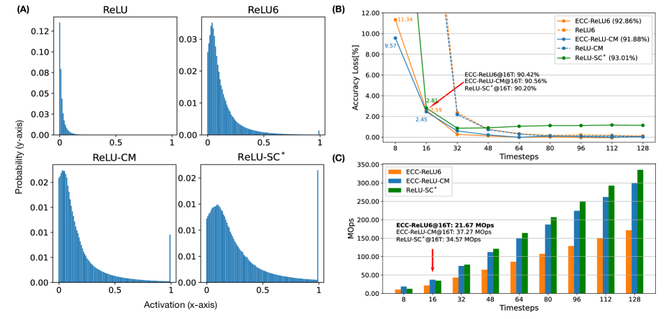
Figure 6: Comparison of SNNs using different clipping methods, ReLU6 ([18, 8]), ReLU-CM ([36]), ReLU-SC* ([4]), for CIFAR-10 on VGG-16. (A) Normalised activation distribution of the first layer. (B) Accuracy w.r.t. timesteps. (C) Energy consumption (MOps) w.r.t. timesteps. *We use ReLU-SC to train an SNN with a fixed timestep (16T), as it does not need extra training.

Figure 6B presents a comparison between SNNs obtained through ReLU6, ReLU-CM and ReLU-SC, with and without the application of ECC. First of all, distribution-aware training can improve the performance. E.g., with clipping methods, the accuracy loss is less than 2.2%@32T, which is better than ECC-SNN (3.2%@32T) as in Figure LABEL:S-fig:TM2017comparison. Then, we can see that, with ECC, ReLU6 and ReLU-CM can achieve 2x less latency with little performance degradation. Although ECC-ReLU6, ECC-ReLU-CM and ReLU-SC achieve similar accuracy (90.20% to 90.56%@16T), ECC-ReLU-CM has the best adaptability to different timesteps. By contrast, ECC-ReLU6 uses 1.5 to 1.7x less operations at 16T than ReLU-SC and ECC-ReLU-CM, as shown in Figure 6C. We only apply ECC to ReLU6 and ReLU-CM, as ReLU-SC in [4] is not designed to be adaptable to different timesteps.

The above results show that distribution-aware CNN training and our ECC method can both improve the CNN-to-SNN conversion. While distribution-aware CNN training can reduce the accuracy loss, the application of ECC method can further improve the performance of the resulting SNN model. Furthermore, it is worth mentioning that ECC can take the advantage of the accumulated bias current to optimise a single SNN model with respect to different timesteps.

6 Discussion

Variants to the Unifying Framework The current unifying framework (Section 3.2) considers ReLU activation function, which exhibits a linear relation between accumulated current and spiking rate. There are other – arguably more natural – features in biological neuron, such as leak, refractory time and adaptive threshold, as discussed in [10]. If considering these features, the relation between accumulated current and spiking rate will become non-linear. To deal with them, it can be an interesting future work to consider extending the unifying framework to address the connection between nonlinear activation functions (e.g., sigmoid) on CNN and the dynamic properties on SNN.

Hyper-parameters in ECC Most of the hyper-parameters in ECC-SNN are determined with reasons, such as $\kappa_{n}$ (Section 3.3.1) and $\eta$ (Section 3.3.2), while timesteps (T) is determined by practical application according to e.g., required accuracy. Although some gradient-based optimisation methods, such as [26, 25, 17], can improve the SNN to a fixed timestep, ECC allows SNN to be adaptive to different timesteps. In the future, we will consider hyper-parameters tuning methods, as in e.g., [22], to further improve ECC-SNN while maintaining its adaptability.

7 Conclusion

We develop a unifying theoretical framework to analyse the conversion from CNNs to SNNs and a new conversion method ECC to explicitly control the currents, so as to optimise accuracy loss, energy efficiency, and latency simultaneously. By comparing with state-of-the-art methods, we confirm the superior performance of our method. Moreover, we study the impact of batch-normalisation, and show the robustness of ECC over quantisation.

Funding

DW is supported by the University of Liverpool and China Scholarship Council Awards (Grant No. 201908320488). This project has received funding from the European Union’s Horizon 2020 research and innovation programme under grant agreement No 956123. It is also supported by the U.K. EPSRC (through End-to-End Conceptual Guarding of Neural Architectures [EP/T026995/1]).

References

- [1] F. Akopyan, J. Sawada, A. Cassidy, R. Alvarez-Icaza, J. Arthur, P. Merolla, N. Imam, Y. Nakamura, Nam Datta, P., G.J., and B. Taba. Truenorth: Design and tool flow of a 65 mw 1 million neuron programmable neurosynaptic chip. EEE transactions on computer-aided design of integrated circuits and systems, 34(10):1537–1557, 2015.
- [2] Y. Cao, Y. Chen, and D. Khosla. Spiking deep convolutional neural networks for energy-efficient object recognition. International Journal of Computer Vision, 113(1):54–66, 2015.
- [3] M. Davies, N. Srinivasa, T.H. Lin, G. Chinya, Y. Cao, S.H. Choday, G. Dimou, P. Joshi, N. Imam, S. Jain, and Y. Liao. Loihi: A neuromorphic manycore processor with on-chip learning. IEEE Micro, 38(1):82–99, 2018.
- [4] Shikuang Deng and Shi Gu. Optimal conversion of conventional artificial neural networks to spiking neural networks. In International Conference on Learning Representations, 2021.
- [5] P.U. Diehl, D. Neil, J. Binas, M. Cook, S.C. Liu, and M. Pfeiffer. Fast-classifying, high-accuracy spiking deep networks through weight and threshold balancing. International Joint Conference on Neural Networks, pages 1–8, 7 2015.
- [6] B. Han, G. Srinivasan, and K. Roy. Rmp-snn: Residual membrane potential neuron for enabling deeper high-accuracy and low-latency spiking neural network. Proceedings of the IEEE/CVF Conference on Computer Vision and Pattern Recognition, pages 13558–13567, 2020.
- [7] Sergey Ioffe and Christian Szegedy. Batch normalization: Accelerating deep network training by reducing internal covariate shift. volume 37 of Proceedings of Machine Learning Research, pages 448–456, Lille, France, 07–09 Jul 2015. PMLR.
- [8] Benoit Jacob, Skirmantas Kligys, Bo Chen, Menglong Zhu, Matthew Tang, Andrew Howard, Hartwig Adam, and Dmitry Kalenichenko. Quantization and training of neural networks for efficient integer-arithmetic-only inference. In Proceedings of the IEEE conference on computer vision and pattern recognition, pages 2704–2713, 2018.
- [9] X. Ju, B. Fang, R. Yan, X. Xu, and H. Tang. An fpga implementation of deep spiking neural networks for low-power and fast classification. Neural computation, 32(1):182–204, 2019.
- [10] Ryota Kobayashi, Yasuhiro Tsubo, and Shigeru Shinomoto. Made-to-order spiking neuron model equipped with a multi-timescale adaptive threshold. Frontiers in computational neuroscience, 3:9, 2009.
- [11] A. Krizhevsky and G. Hinton. Learning multiple layers of features from tiny images. 2009 IEEE conference on computer vision and pattern recognition, 2009.
- [12] Alexander Kugele, Thomas Pfeil, Michael Pfeiffer, and Elisabetta Chicca. Efficient processing of spatio-temporal data streams with spiking neural networks. Frontiers in Neuroscience, 14:439, 2020.
- [13] Y. LeCun, B. Boser, J.S. Denker, D. Henderson, R.E. Howard, W. Hubbard, and L.D. Jackel. Backpropagation applied to handwritten zip code recognition. Neural computation, 4(1):541–551, 1989.
- [14] C. Lee, S.S. Sarwar, P. Panda, G. Srinivasan, and K. Roy. Enabling spike-based backpropagation for training deep neural network architectures. Frontiers in Neuroscience, 14, 2020.
- [15] J.H. Lee, T. Delbruck, and M. Pfeiffer. Training deep spiking neural networks using backpropagation. Frontiers in neuroscience, 10:508, 11 2016.
- [16] Hongmin Li, Hanchao Liu, Xiangyang Ji, Guoqi Li, and Luping Shi. Cifar10-dvs: an event-stream dataset for object classification. Frontiers in neuroscience, 11:309, 2017.
- [17] Yuhang Li, Shikuang Deng, Xin Dong, Ruihao Gong, and Shi Gu. A free lunch from ann: Towards efficient, accurate spiking neural networks calibration. In Marina Meila and Tong Zhang, editors, Proceedings of the 38th International Conference on Machine Learning, volume 139 of Proceedings of Machine Learning Research, pages 6316–6325. PMLR, 18–24 Jul 2021.
- [18] Ji Lin, Chuang Gan, and Song Han. Defensive quantization: When efficiency meets robustness. arXiv preprint arXiv:1904.08444, 2019.
- [19] Sen Lu and Abhronil Sengupta. Exploring the connection between binary and spiking neural networks. Frontiers in Neuroscience, 14:535, 2020.
- [20] P.A. Merolla, J.V. Arthur, R. Alvarez-Icaza, A.S. Cassidy, J. Sawada, F. Akopyan, B.L. Jackson, N. Imam, C. Guo, Y. Nakamura, and B. Brezzo. A million spiking-neuron integrated circuit with a scalable communication network and interface. Science, 345(6197):668–673, 2014.
- [21] E. Painkras, L.A. Plana, J. Garside, S. Temple, S. Davidson, J. Pepper, D. Clark, C. Patterson, and S. Furber. Spinnaker: A multi-core system-on-chip for massively-parallel neural net simulation. NaIn Proceedings of the IEEE 2012 Custom Integrated Circuits Conference, (7767):1–4, 9 2012.
- [22] Maryam Parsa, John P Mitchell, Catherine D Schuman, Robert M Patton, Thomas E Potok, and Kaushik Roy. Bayesian multi-objective hyperparameter optimization for accurate, fast, and efficient neural network accelerator design. Frontiers in neuroscience, 14:667, 2020.
- [23] J. Pei, L. Deng, S. Song, M. Zhao, Y. Zhang, S. Wu, G. Wang, Z. Zou, Z. Wu, W. He, and F. Chen. Towards artificial general intelligence with hybrid tianjic chip architecture. Nature, 572(7767):106–111, 2019.
- [24] M. Pfeiffer and T. Pfeil. Deep learning with spiking neurons: opportunities and challenges. Frontiers in neuroscience, 12:774, 2018.
- [25] Nitin Rathi and Kaushik Roy. Diet-snn: A low-latency spiking neural network with direct input encoding and leakage and threshold optimization. IEEE Transactions on Neural Networks and Learning Systems, 2021.
- [26] Nitin Rathi, Gopalakrishnan Srinivasan, Priyadarshini Panda, and Kaushik Roy. Enabling deep spiking neural networks with hybrid conversion and spike timing dependent backpropagation. In International Conference on Learning Representations, 2020.
- [27] B. Rueckauer, I.A. Lungu, M. Hu, Y.and Pfeiffer, and S.C. Liu. Conversion of continuous-valued deep networks to efficient event-driven networks for image classification. Frontiers in neuroscience, 11:682, 2017.
- [28] Olga Russakovsky, Jia Deng, Hao Su, Jonathan Krause, Sanjeev Satheesh, Sean Ma, Zhiheng Huang, Andrej Karpathy, Aditya Khosla, Michael Bernstein, Alexander C. Berg, and Li Fei-Fei. ImageNet Large Scale Visual Recognition Challenge. International Journal of Computer Vision (IJCV), 115(3):211–252, 2015.
- [29] Shibani Santurkar, Dimitris Tsipras, Andrew Ilyas, and Aleksander Madry. How does batch normalization help optimization? In NeurIPS, pages 2488–2498, 2018.
- [30] Catherine D Schuman, J Parker Mitchell, Robert M Patton, Thomas E Potok, and James S Plank. Evolutionary optimization for neuromorphic systems. In Proceedings of the Neuro-inspired Computational Elements Workshop, pages 1–9, 2020.
- [31] Abhronil Sengupta, Yuting Ye, Robert Wang, Chiao Liu, and Kaushik Roy. Going deeper in spiking neural networks: Vgg and residual architectures. Frontiers in neuroscience, 13:95, 2019.
- [32] K. Simonyan and A. Zisserman. Very deep convolutional networks for large-scale image recognition. arXiv:1409.1556, 2014.
- [33] Nicholas Soures and Dhireesha Kudithipudi. Spiking reservoir networks: Brain-inspired recurrent algorithms that use random, fixed synaptic strengths. IEEE Signal Processing Magazine, 36(6):78–87, 2019.
- [34] V. Sze, Y.H. Chen, T.J. Yang, and J.S. Emer. Efficient processing of deep neural networks: A tutorial and survey. Proceedings of the IEEE, 105(12):2295–2329, 2019.
- [35] Hao Wu, Yueyi Zhang, Wenming Weng, Yongting Zhang, Zhiwei Xiong, Zheng-Jun Zha, Xiaoyan Sun, and Feng Wu. Training spiking neural networks with accumulated spiking flow. In Proceedings of the AAAI Conference on Artificial Intelligence, 2021.
- [36] Haibao Yu, Tuopu Wen, Guangliang Cheng, Jiankai Sun, Qi Han, and Jianping Shi. Low-bit quantization needs good distribution. In Proceedings of the IEEE/CVF Conference on Computer Vision and Pattern Recognition Workshops, pages 680–681, 2020.