Mixed variational formulations for structural topology optimization based on the phase-field approach

Abstract

We propose a variational principle combining a phase-field functional for structural topology optimization with a mixed (three-field) Hu-Washizu functional, then including directly in the formulation equilibrium, constitutive, and compatibility equations. The resulting mixed variational functional is then specialized to derive a classical topology optimization formulation (where the amount of material to be distributed is an a priori assigned quantity acting as a global constraint for the problem) as well as a novel topology optimization formulation (where the amount of material to be distributed is minimized, hence with no pre-imposed constraint for the problem).

Both formulations are numerically solved by implementing a mixed finite element scheme, with the second approach avoiding the introduction of a global constraint, hence respecting the convenient local nature of the finite element discretization. Furthermore, within the proposed approach it is possible to obtain guidelines for settings proper values of phase-field-related simulation parameters and, thanks to the combined phase-field and Hu-Washizu rationale, a monolithic algorithm solution scheme can be easily adopted.

An insightful and extensive numerical investigation results in a detailed convergence study and a discussion on the obtained final designs. The numerical results clearly highlight differences between the two formulations as well as advantages related to the monolithic solution strategy; numerical investigations address both two-dimensional and three-dimensional applications.

1 Introduction

Having assigned a design region, a load distribution, and suitable boundary conditions, the goal of structural topology optimization is to identify an optimal distribution of material within the design region. Classically, optimality is reached when the obtained material distribution minimizes a measure of structural compliance and satisfies mechanical equilibrium. The minimization of structural compliance is in general expressed in terms of the work done by the assigned (assumed to be constant) load distribution by the corresponding displacements.

Several methods have been developed in order to solve topology optimization problems. Originally, a discrete formulation was introduced where areas of dense material and voids are alternated without any transition region (Bendsøe, 1983). Known as 0-1 topology optimization problem, this first approach also leads to many difficulties both from an analytical and a numerical point of view (Sigmund and Petersson, 1998).

Possible alternative approaches are based on homogenization methods, where the macroscopic material properties are obtained from microscopic porous material characteristics (Allaire et al., 2004; Suzuki and Kikuchi, 1991), or on the Solid Isotropic Material Penalization (SIMP) method (Zhou and Rozvany, 1991), which consists of penalizing the density region, different from the void or bulk material, by choosing a suitable interpolation scheme for material properties at the macroscopic scale (Bendsøe and Sigmund, 1999; Bendsøe, 1983). Another approach used by many authors (cf., e.g., Burger, 2003; Osher and Santosa, 2001) is the level set method, that allows for topology changes but presents difficulties in creating holes.

An alternative to SIMP and level set is based on the phase-field method, for the first time introduced by Bourdin and Chambolle (2003) and successively employed by Burger and Stainko (2006) for stress constrained problems as well as by Takezawa et al. (2010) for minimum compliance and eigenfrequency maximization problems. More recently, Penzler et al. (2012) have solved nonlinear elastic problems by means of the phase-field approach, while Dedè et al. (2012) have applied this method in the context of isogeometric topology optimization.

The phase-field approach delivers an efficient method to solve the free boundary problem stemming from the fact that the boundary of the region filled by the material is unknown. Phase-field topology optimization penalizes an approximation of the interface perimeter in such a way that, by choosing a very small positive penalty term, one can obtain a sharp interface region separating solid materials and voids (Blank et al., 2014a). The phase-field approach to structural optimization problems has been recently used by different authors (cf., e.g., Auricchio et al., 2019; Carraturo et al., 2019; Blank et al., 2014b), the main advantage being the fact that it allows to handle topology changes as well as nucleation of new holes. Moreover, especially for three-dimensional applications, another advantage is that the phase-field approach produces regular patterns in the design domain that require little post-processing effort to interpret results (Deaton and Grandhi, 2014). On the other hand, density-based topology optimization approaches (e.g., based on SIMP or power-laws) require post-processing filtering for translating results in manufacturable data, which may result case- and user-dependent and might lead to undesirable effects, like an artificial increase of the final volume fraction (Zegard and Paulino, 2016).

Although promising results have been obtained on phase-field topology optimization, there are still some key aspects which merit further investigation. Firstly, the adopted values of phase-field-related parameters affect both the obtained topology distribution and the convergence behavior of the numerical solution; hence, selecting proper values of these parameters for the specific problem at hand requires a time-consuming preliminary set of investigations.

Furthermore, traditional schemes for topology optimization problems generally fix the amount of material to be distributed in the design region, amount which acts as a global constraint in the optimization process. This gold-standard strategy is easy to implement, since it adds only a single global equation in the computation; however, when the evolution of the topology is itself the solution of a finite element computation, the presence of such a global constraint requires to introduce global variables, altering the intrinsic element-based subdivision of the spatial discretization and introducing a coupling term between all elements. As an obvious consequence, the usual banded structure of the tangent stiffness matrix is altered and such an increase of the band-width of the tangent stiffness matrix might have consequences on the convergence rate of topology optimization procedures. Currently, the literature is missing a formulation which involves only local constraints for enforcing/minimizing the amount of material to be distributed.

An additional issue of high interest is related to classically adopted numerical solution schemes. These are generally based on staggered algorithms: the evolution of the phase-field variable is obtained without the respect of the equilibrium, which is restored at the successive incremental step wherein the phase-field variable is instead frozen. In the framework of topology optimization, such an approach is referred to as Nested Analysis and Design (NAND). Allowing for the use of existing FE packages, NAND is easy and convenient to implement and it is often preferred also as a consequence of the presence of the global constraint. Nevertheless, NAND can be computationally demanding, especially in the presence of non-linearities and for large-scale problems. On the other hand, a Simultaneous Analysis and Design (SAND) approach treats the optimization design (e.g., phase field) and equilibrium (e.g., displacement) unknowns simultaneously. In other words, the combined optimization and equilibrium problem is solved in a monolithic way by considering the evolution of topology and equilibrium conditions in a single optimization routine. Despite the fact that SAND may be competitive with respect to conventional NAND schemes, to the best of authors’ knowledge, SAND (monolithic) approaches are still largely to be explored, as compared with the more classical NAND (staggered) solution strategies.

Finally, the phase-field variable should be physically bounded in the range $[0,1]$. To enforce this constraint, the phase-field variable obtained from the solution of the topology evolution equation (which possibly lies outside the admissible bound) is generally projected on the admissible set at each step of the iterative solution procedure. This strategy obviously alters stationary. A variational formulation allowing for the direct enforcement of the physical bounds, without any ad hoc algorithmic solution, would be more consistent.

Accordingly, in the described context of literature and open problems, the goals of the present paper are the following ones.

• To propose a mixed variational principle combining a phase-field functional for topology optimization with a (three-field) Hu-Washizu functional, then including directly in the formulation equilibrium, constitutive, and compatibility equations. The variational formulations includes also a penalization term to directly enforce that the phase-field variable lies within the admissible physical bound $[0,1]$;

• To specialize the mixed variational functional to a classical formulation for the topology optimization problem, referred to as formulation with volume constraint. Here, the amount of material to be distributed within the design domain is imposed a priori, acting as a global constraint and operating on the global stiffness matrix of the corresponding finite element formulation;

• To propose a novel formulation for the topology optimization problem, leading at the same time to a volume minimization. The amount of material is not imposed a priori by means of a global constraint, but rather related to a cost of the material, which is minimized together with the structural compliance. Such an approach avoids the introduction of a global constraint, respecting the convenient local nature of the finite element discretization;

• To implement the proposed variational formulations in the context of mixed finite elements. Thanks to the combined phase-field and Hu-Washizu rationale, a SAND monolithic algorithm is proposed, allowing to compute the evolution law of the phase-field variable under the respect of equilibrium;

• To trace general guidelines for fixing the values of phase-field-related simulation parameters. In addition, a theoretical estimate for setting the cost of the material (which plays the role of a mass penalty parameter) in the volume minimization formulation as function of a target desired solution is proposed and verified;

• To perform a comparative analysis in terms of both computational efficiency and obtained final designs for monolithic and staggered solution strategies as well as for the two investigated formulations.

• To show the effectiveness of the proposed volume minimization formulation and its finite element mixed implementation both in two-dimensional and three-dimensional applications.

2 Theory

2.1 Introductory settings

We indicate the design region with $\Omega\subset{\mathcal{R}}^{n}$ (with $n=2$ or $n=3$), characterized by a volume $V$, defined as:

$$V=\int_{\Omega}\>d\Omega\,.$$ (2.1)

The material distribution within $\Omega$ is described by a scalar phase variable $\phi$, ideally a binary field (i.e., either 0 or $1$), with $\phi=0$ corresponding to the absence of material (i.e., void or no material), and $\phi=1$ corresponding to the presence of material. After topology optimization, the material distributed inside the design region $\Omega$ occupies a (dimensionless) volume fraction $v$ of the total volume $V$, defined as:

$$v=\frac{1}{V}\int_{\Omega}\phi\>d\Omega\,.$$ (2.2)

However, since a binary (i.e., either 0 or $1$) phase parameter $\phi$ would call for sharp interfaces (between the region with material, i.e., with $\phi=1$, and the region with no material, i.e., with $\phi=0$) and since problems with infinitely sharp interfaces are in general difficult to numerically treat and solve, as classically done, we consider the phase parameter $\phi$ as a continuous real value field, with values in the interval $[0,1]$. Ideally, the optimal phase variable $\phi$ should be close to an ideal binary field.

2.2 Elastic problem

Limiting the discussion to the case of linear elastic materials, given a material distribution $\phi:\Omega\to[0,1]$, the elastic problem (equilibrium, constitutive, and compatibility field equations, in combination with boundary conditions) can be expressed as:

$$\left\{\begin{aligned} &\text{div }\boldsymbol{\sigma}+\phi\boldsymbol{b}=\boldsymbol{0}&\hskip 14.22636pt\text{in}\hskip 14.22636pt&\Omega\\ &\boldsymbol{\sigma}=\mathbb{C}(\phi)\boldsymbol{\varepsilon}&\hskip 14.22636pt\text{in}\hskip 14.22636pt&\Omega\\ &\boldsymbol{\varepsilon}=\nabla^{s}\boldsymbol{u}&\hskip 14.22636pt\text{in}\hskip 14.22636pt&\Omega\\ &\boldsymbol{u}=\boldsymbol{0}&\hskip 14.22636pt\text{on}\hskip 14.22636pt&\Gamma_{D}\\ &\boldsymbol{t}=\boldsymbol{\sigma}\boldsymbol{n}&\hskip 14.22636pt\text{on}\hskip 14.22636pt&\Gamma_{N}\,,\end{aligned}\right.$$ (2.3)

with $\boldsymbol{\sigma}$ the stress tensor field, $\boldsymbol{b}$ the applied body-force density vector field per unit volume, $\mathbb{C}(\phi)$ a positive-definite material elastic tensor function of the phase variable $\phi$, $\boldsymbol{\varepsilon}$ the strain tensor field, $\boldsymbol{u}$ the displacement vector field, div and $\nabla^{s}$ the divergence and the symmetric gradient operators, $\Gamma_{D}$ the region of $\partial\Omega$ where we apply Dirichlet boundary conditions (assumed to be homogeneous), $\Gamma_{N}$ the region of $\partial\Omega$ where we apply Neumann boundary conditions with $\boldsymbol{t}$ the surface load vector and $\boldsymbol{n}$ the outward-pointing versor normal to $\Gamma_{N}$.

The elastic problem can be classically condensed in just one field equation in terms of displacements (referred to as Navier’s equation), as follows:

$$\left\{\begin{aligned} &\text{div }\left[\mathbb{C}(\phi)\nabla^{s}\boldsymbol{u}\right]+\phi\boldsymbol{b}=\boldsymbol{0}&\hskip 14.22636pt\text{in}\hskip 14.22636pt&\Omega\\ &\boldsymbol{u}=\boldsymbol{0}&\hskip 14.22636pt\text{on}\hskip 14.22636pt&\Gamma_{D}\\ &\boldsymbol{t}=\mathbb{C}(\phi)\nabla^{s}\boldsymbol{u}\,\boldsymbol{n}&\hskip 14.22636pt\text{on}\hskip 14.22636pt&\Gamma_{N}\,.\end{aligned}\right.$$ (2.4)

Assuming voids to be modeled as a very soft material, in the present work we adopt the following expression for $\mathbb{C}(\phi)$:

$$\mathbb{C}(\phi)=\left[\delta+(1-\delta)\frac{\text{Exp}(p\phi^{p})}{\text{Exp}(p)}\right]\mathbb{C}_{A}\,,$$ (2.5)

where $\mathbb{C}_{A}$ is a constant positive-definite material elastic tensor (assumed to describe an isotropic behaviour with Young’s modulus $E_{A}$ and Poisson’s ratio $\nu_{A}$) corresponding to the solid dense material, $p$ can be any positive value, and $0<\delta\ll 1$ governs the low (but non-null) stiffness of the voids. Equation (2.5) is such that $\mathbb{C}(1)=\mathbb{C}_{A}$ and $\mathbb{C}(0)\rightarrow\delta\mathbb{C}_{A}$ for $p\rightarrow+\infty$; as an example, $p=10$ already corresponds to $\|\mathbb{C}(0)-\delta\mathbb{C}_{A}\|<10^{-4}$.

It is worth highlighting that the particular choice of $\mathbb{C}(\phi)$ from Equation (2.5) is different from state-of-the-art expressions, which generally might read as one of the following:

$$\mathbb{C}^{1}(\phi)=\left[\phi^{p}+\delta(1-\phi)^{p}\right]\mathbb{C}_{A}\,,$$ (2.6a)

$$\mathbb{C}^{2}(\phi)=\left[\phi\mathbb{C}_{A}^{-1}+(1-\phi)\left(\delta\mathbb{C}_{A}\right)^{-1}\right]^{-1}\,.$$ (2.6b)

As shown in Fig. 1 for their scalar counterparts, these lasts expressions either bring to non-monotonic expressions (i.e., $\mathbb{C}^{1}(\phi)$) or fast diverge as soon as $\phi$ exceeds the admissible range $[0,1]$ (i.e., $\mathbb{C}^{2}(\phi)$). On the one hand, a monotonically increasing behaviour would be beneficial in terms of stability of the ensuing numerical scheme and it would be more consistent from the physical point of view. On the other hand, a smooth behaviour outside the admissible range would be beneficial because the property $\phi\in[0,1]$ is sometimes violated in numerical iterative solution schemes, often requiring an ad hoc truncation of the stiffness matrix or of the phase-field variable, and hence introducing non-smoothness effects.

The expression proposed in Eq. (2.5) and adopted in this work allows to overcome drawbacks inherited by definitions in Eq. (2.6) (see Fig. 1). In fact, $\mathbb{C}(\phi)$ turns out to be monotonically increasing, everywhere-defined, and uniformly positive-definite for all $\phi$, being at the same time smooth with all its derivatives. In addition, our choice for $\mathbb{C}(\phi)$ entails that the elastic energy density $(\phi,\boldsymbol{\varepsilon})\mapsto\mathbb{C}(\phi)\boldsymbol{\varepsilon}:\boldsymbol{\varepsilon}/2$ is convex, contributing to the stability of the approximation.

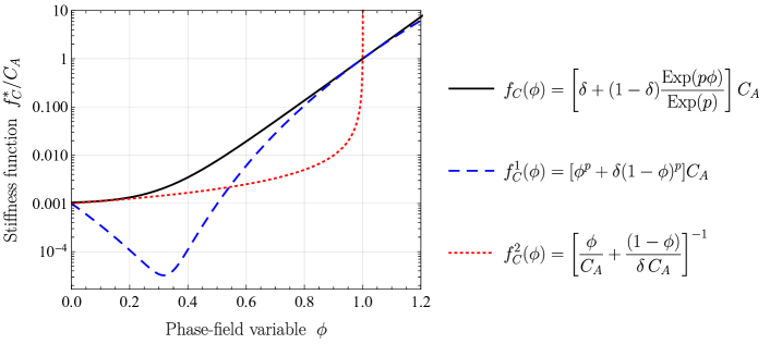
Figure 1: Stiffness function laws: $f_{C}^{1}(\phi)$, scalar counterpart of Eq. (2.6a); $f_{C}^{2}(\phi)$, scalar counterpart of Eq. (2.6b); and $f_{C}(\phi)$, scalar counterpart of the proposed expression (2.5). Parameters: $C_{A}=10$, $\delta=10^{-3}$ and $p=10$.

2.3 Topology optimization

The goal of topology optimization is then to design an optimal structure, i.e., to identify the optimal material distribution $\phi$, such that structural compliance is minimized when solving the elastic problem. We introduce the structural compliance $\mathcal{C}$, with the unit of measure of a work, as:

$$\mathcal{C}(\phi,\boldsymbol{u})=\int_{\Omega}\phi\boldsymbol{b}\cdot\boldsymbol{u}\>d\Omega+\int_{\Gamma_{N}}\boldsymbol{t}\cdot\boldsymbol{u}\>d\Gamma\,,$$ (2.7)

where $\boldsymbol{b}$ and $\boldsymbol{t}$ are the actual body and surface loads (assumed to be constant), while $\boldsymbol{u}$ is the displacement, satisfying the elastic problem (2.4).

Accordingly, the topology optimization problem can be written as:

$${\text{min}_{\phi}}\{\mathcal{C}(\phi,\boldsymbol{u})\ :\ \boldsymbol{u}\ \text{solves}\ \ \eqref{eq:equilibrium}\ \text{given}\ \phi\}\,.$$ (2.8)

It should be remarked that in (2.4) the boundary conditions are defined on a fixed subset of $\partial\Omega$. Once a solution is numerically obtained, one has to check whether $\phi\not=0$ at least on some portion of $\Gamma_{D}$ and $\Gamma_{N}$. This generally follows from minimality. In particular, it is fulfilled by all our computations.

2.4 Phase-field topology optimization

As mentioned, the phase parameter $\phi$ is allowed to take values in the interval $[0,1]$ and, accordingly, the region where $0<\phi<1$ corresponds to a smooth material interface, representing a transition from void to solid material. To introduce a measure of the extension or the thickness of such a transition interface and to favor fields taking values as close as possible to $0$ or $1$, we introduce a new functional $\mathcal{P}$ to be minimized, defined as:

$$\mathcal{P}(\phi)=\int_{\Omega}\left[\frac{\gamma_{\phi}}{2}\|\nabla\phi\|^{2}+\frac{1}{\gamma_{\phi}}\psi_{0}(\phi)\right]\>d\Omega\,,$$ (2.9)

where $\gamma_{\phi}>0$ is the thickness penalization parameter (with the unit of measure of a length) and $\psi_{0}$ is the double-well potential function, defined as:

$$\psi_{0}(\phi)=\left[\phi\left(\phi-1\right)\right]^{2}\,.$$ (2.10)

For small values of $\gamma_{\phi}$, the minimization of $\mathcal{P}(\phi)$ penalizes oscillatory material distributions and favours continuous fields $\phi$ taking values close to $0$ or $1$. For $\gamma_{\phi}\to 0$, the quantity $\mathcal{P}(\phi)$ converges in the sense of $\Gamma$-limits to the perimeter functional (cf. Modica (1987)), namely a measure of the perimeter of the interfaces between regions with material ($\phi=1$) and regions with no material ($\phi=0$).

In the following we augment the compliance functional $\mathcal{C}$ by a multiple of $\mathcal{P}$, introducing the functional $\mathcal{J}$, defined as:

$$\mathcal{J}(\phi,\boldsymbol{u})=\mathcal{C}(\phi,\boldsymbol{u})+\kappa_{\phi}\mathcal{P}(\phi),$$ (2.11)

where the perimeter stiffness parameter $\kappa_{\phi}>0$ (force divided by length) measures the mutual relevance of structural compliance and perimeter in the minimization.

Accordingly, the phase-field topology optimization problem can be written as:

$${\text{min}_{\phi}}\{\mathcal{J}(\phi,\boldsymbol{u})\ :\ \boldsymbol{u}\ \text{solves}\ \ \eqref{eq:equilibrium}\ \text{given}\ \phi\}\,,$$ (2.12)

2.5 Phase-field constraint

We start recalling that ideally the phase-field variable $\phi$ should be as much as possible a binary field but also that any value outside the interval, i.e., $\phi\notin[0,1]$, is physically meaningless and it can be the source of numerical instabilities. The minimisation of $\mathcal{J}$ in Eq. (2.12) already favors $\phi$ to be close to 0 or 1 through the presence of $\psi_{0}$, but $\phi\in[0,1]$ just in the limit as $\gamma_{\phi}\to 0$; for all $\gamma_{\phi}>0$ (which is the case of any numerically-obtained solution) the constraint $\phi\in[0,1]$ does not necessarily hold through the minimisation of $\mathcal{J}$.

With these concepts in mind, it is clear why in most iterative schemes available in the topology optimization literature the variable $\phi$ is projected onto the admissible range $[0,1]$ at each step, however violating the stationary conditions of the corresponding adopted functional.

As an alternative, we propose to further augment the functional $\mathcal{J}$ by a contribution $\mathcal{B}$, defined as:

$$\mathcal{B}(\phi)=\int_{\Omega}\,b(\phi)d\Omega\,,\quad\text{ with }\;b(\phi)=\begin{cases}\dfrac{(\phi-1)^{2}}{2}&\phi>1\\ 0&0\leq\phi\leq 1\\ \dfrac{\phi^{2}}{2}&\phi<0\end{cases}\,,$$ (2.13)

and modulated by a bounding stiffness parameter $\kappa_{b}>0$ (force per unit area).

2.6 Formulation with volume constraint

As classically found in the literature, we may now constrain the topology optimization problem so that the portion $v$ of material to be distributed inside the design domain $\Omega$ is equal to an a priori given (dimensionless) material fraction $\overline{v}\in[0,1]$, defined as:

$$v=\frac{1}{V}\int_{\Omega}\phi\>d\Omega=\overline{v}.$$ (2.14)

The corresponding topology optimization problem reads as:

$${\text{min}_{\phi}}\{\mathcal{J}(\phi,\boldsymbol{u})+\kappa_{b}{\mathcal{B}}(\phi)\ :\ \boldsymbol{u}\ \text{solves}\ \ \eqref{eq:equilibrium}\ \text{given}\ \phi\ \text{and}\ v=\overline{v}\}.$$ (2.15)

Before moving on, we wish to remark that problem (2.15) can be equivalently rewritten as

$${\text{min}_{\phi}}\Bigg{\{}\int_{\Omega}\mathbb{C}(\phi)\nabla^{s}\boldsymbol{u}:\nabla^{s}\boldsymbol{u}+\kappa_{\phi}{\mathcal{P}}(\phi)+\kappa_{b}{\mathcal{B}}(\phi)+\frac{\kappa_{v}}{2}\int_{\Omega}\phi^{2}\>d\Omega\ :$$

$$\qquad\qquad\qquad\qquad\boldsymbol{u}\ \text{solves}\ \ \eqref{eq:equilibrium}\ \text{given}\ \phi\ \text{and}\ v=\overline{v}\Bigg{\}}\,.$$ (2.16)

Our specific choice (2.5) for $\mathbb{C}$ makes the functional under minimization to be convex, up to the lower-order $\psi_{0}$-term in ${\mathcal{P}}(\phi)$.

We propose to solve the above minimization problems by investigating the stationarity of the Lagrangian $\mathcal{L}^{vc}$, defined as:

$$\mathcal{L}^{vc}(\phi,\lambda,\boldsymbol{u},\boldsymbol{\sigma},\boldsymbol{\varepsilon})= \mathcal{J}(\phi,\boldsymbol{u})+\kappa_{b}\mathcal{B}(\phi)-\mathcal{E}^{el}(\boldsymbol{\varepsilon},\phi)+$$

$$+\int_{\Omega}\boldsymbol{\sigma}:(\boldsymbol{\varepsilon}-\nabla^{s}\boldsymbol{u})\>d\Omega+\lambda\left[\int_{\Omega}(\phi-\overline{v})\>d\Omega\right],$$ (2.17)

where $\mathcal{E}^{el}$ is the elastic energy, defined as:

$$\mathcal{E}^{el}(\boldsymbol{\varepsilon},\phi)=\frac{1}{2}\int_{\Omega}\mathbb{C}(\phi)\boldsymbol{\varepsilon}:\boldsymbol{\varepsilon}\,d\Omega.$$ (2.18)

The superscript $vc$ in $\mathcal{L}^{vc}$ recalls that we are here considering a volume-constrained formulation.

2.7 Formulation with volume minimization

Instead of prescribing a priori a fraction of material $\overline{v}$ to be distributed in the design domain $\Omega$, we may aim at exploring what is the minimum amount of material $v$ we could distribute. In terms of minimization, a corresponding topology optimization problem would read

$${\text{min}_{\phi}}\left\{\mathcal{J}(\phi,\boldsymbol{u})+\kappa_{b}{\mathcal{B}}(\phi)+\frac{\kappa_{v}}{2}\int_{\Omega}\phi^{2}\>d\Omega\ :\ \boldsymbol{u}\ \text{solves}\ \ \eqref{eq:equilibrium}\ \text{given}\ \phi\right\}\,,$$ (2.19)

where $\kappa_{v}>0$ is a volume penalty parameter (force per unit area), representing for example a measure of the “cost” of the material per unit volume.

It is interesting to emphasize that in (2.19) we are not minimizing the amount of material $v$ to be distributed, but rather $\int_{\Omega}\phi^{2}\>d\Omega$; this choice makes the problem more stable and it can be proved to be equivalent to minimize $v$, as long as $\phi$ exclusively takes values $0$ or $1$. As for the volume-constrained case, problem (2.19) can be equivalently rewritten as

$${\text{min}_{\phi}}\Bigg{\{}\int_{\Omega}\mathbb{C}(\phi)\nabla^{s}\boldsymbol{u}:\nabla^{s}\boldsymbol{u}+\kappa_{\phi}{\mathcal{P}}(\phi)+\kappa_{b}{\mathcal{B}}(\phi)+\frac{\kappa_{v}}{2}\int_{\Omega}\phi^{2}\>d\Omega\ :$$

$$\qquad\qquad\qquad\boldsymbol{u}\ \text{solves}\ \ \eqref{eq:equilibrium}\ \text{given}\ \phi\Bigg{\}}\,.$$ (2.20)

Again, the choice (2.5) for $\mathbb{C}$ makes the functional under minimization to be convex, up to the lower-order $\psi_{0}$-term in ${\mathcal{P}}(\phi)$.

We propose to solve the topology optimization problem (2.19) by looking at the stationarity of the Lagrangian $\mathcal{L}^{vm}$, defined as:

$$\mathcal{L}^{vm}(\phi,\boldsymbol{u},\boldsymbol{\sigma},\boldsymbol{\varepsilon})=\mathcal{J}(\phi,\boldsymbol{u})+\kappa_{b}\mathcal{B}(\phi)-\mathcal{E}^{el}(\boldsymbol{\varepsilon},\phi)+\int_{\Omega}\boldsymbol{\sigma}:(\boldsymbol{\varepsilon}-\nabla^{s}\boldsymbol{u})\>d\Omega+\frac{\kappa_{v}}{2}\int_{\Omega}\phi^{2}\>d\Omega.$$ (2.21)

The superscript $vm$ in $\mathcal{L}^{vm}$ recalls that we are looking at a volume-minimization formulation.

3 Stationarity conditions and algorithmic consideration

3.1 Formulation with volume constraint

To compute a stationary point of the Lagrangian $\mathcal{L}^{vc}$ (2.17), we set its variations to zero, i.e.:

$$\left\{\begin{aligned} D_{\delta\phi}\mathcal{L}^{vc}&=\int_{\Omega}\delta\phi\boldsymbol{b}\cdot\boldsymbol{u}\>d\Omega+\kappa_{\phi}\int_{\Omega}\left[\gamma_{\phi}\nabla\phi\cdot\nabla\delta\phi+\frac{1}{\gamma_{\phi}}\frac{\partial\psi_{0}}{\partial\phi}\delta\phi\right]\>d\Omega+\kappa_{b}\int_{\Omega}\frac{\partial b}{\partial\phi}\delta\phi\>d\Omega\\ &-\mathcal{E}^{el}_{,\phi}(\phi,\boldsymbol{\varepsilon})+\lambda\int_{\Omega}\delta\phi\>d\Omega=0\\ D_{\delta\lambda}\mathcal{L}^{vc}&=\delta\lambda\left[\int_{\Omega}(\phi-\overline{v})\>d\Omega\right]=0\\ D_{\delta\boldsymbol{u}}\mathcal{L}^{vc}&=\int_{\Omega}\delta\boldsymbol{u}\cdot\phi\boldsymbol{b}\>d\Omega+\int_{\Gamma_{N}}\delta\boldsymbol{u}\cdot\boldsymbol{t}\>d\Gamma-\int_{\Omega}\nabla^{s}\delta\boldsymbol{u}:\boldsymbol{\sigma}\>d\Omega=0\\ D_{\delta\boldsymbol{\sigma}}\mathcal{L}^{vc}&=\int_{\Omega}\delta\boldsymbol{\sigma}:\left(\boldsymbol{\varepsilon}-\nabla^{s}\boldsymbol{u}\right)\>d\Omega=0\\ D_{\delta\boldsymbol{\varepsilon}}\mathcal{L}^{vc}&=\int_{\Omega}\delta\boldsymbol{\varepsilon}:\left(\boldsymbol{\sigma}-\mathbb{C}(\phi)\boldsymbol{\varepsilon}\right)d\Omega=0\,,\end{aligned}\right.$$ (3.22)

where

$$\mathcal{E}^{el}_{,\phi}(\phi,\boldsymbol{\varepsilon})=\int_{\Omega}e^{el}_{,\phi}(\phi,\boldsymbol{\varepsilon})\,\delta\phi\>d\Omega\quad\text{with}\quad e^{el}_{,\phi}(\phi,\boldsymbol{\varepsilon})=\frac{1}{2}\mathbb{C}^{\prime}(\phi)\boldsymbol{\varepsilon}:\boldsymbol{\varepsilon}\;\text{ and }\;\mathbb{C}^{\prime}(\phi)=\frac{\partial\mathbb{C}}{\partial\phi}\,.$$ (3.23)

We recall that the last three relations in Eq. (3.22) are, respectively, the equilibrium, the compatibility, and the constitutive equations, which are then automatically enforced through the stationarity of $\mathcal{L}^{vc}$.

Equations (3.22) can be rewritten in a residual form as:

$$\boldsymbol{R}^{vc}(\phi,\lambda,\boldsymbol{u},\boldsymbol{\sigma},\boldsymbol{\varepsilon})=\boldsymbol{0}\,.$$ (3.24)

To solve such a residual system using an iterative scheme, a good starting point could be to set $\phi(\boldsymbol{X})=c\leq 1\;\forall\boldsymbol{X}\in\Omega$, i.e., to consider a design domain homogeneously covered by a partially dense material. Natural choices are $c=0.5$ or $c=\overline{v}$.

In addition, one can follow a classical Allen-Cahn-like approach by introducing a gradient-flow dynamics. To do so, the phase-field variable $\phi$ is assumed to be dependent on a pseudo-time variable $t$, i.e., $\phi=\phi(\boldsymbol{X},t)$, and the new Allen-Cahn volume-constraint Lagrangian $\mathcal{L}^{vc}_{AC}$ is introduced:

$$\mathcal{L}^{vc}_{AC}=\frac{\tilde{\tau}_{\phi}}{2}\int_{\Omega}\dot{\phi}^{2}\>d\Omega+\mathcal{L}^{vc}\,,$$ (3.25)

where the parameter $\tilde{\tau}_{\phi}>0$ (unit of measure of force times squared time per unit area) represents viscosity with respect to the pseudo-time $t$. Exploring the stationary condition of $\mathcal{L}^{vc}_{AC}$ with respect to $\phi$ (assuming $\delta\phi$ to be independent from $t$) returns the condition:

$$D_{\delta\phi}\mathcal{L}^{vc}_{AC}=\tilde{\tau}_{\phi}\int_{\Omega}\dot{\phi}\,\delta\dot{\phi}\>d\Omega+D_{\delta\phi}\mathcal{L}^{vc}=0\,.$$ (3.26)

At the time-discrete level, denoting with a subscript $n$ quantities evaluated at the previous time $t_{n}$ and with no subscript quantities evaluated at the current time $t_{n+1}$, we obtain:

$$D_{\delta\phi}\mathcal{L}^{vc}_{AC}=\tau_{\phi}\int_{\Omega}\frac{\phi-\phi_{n}}{\Delta t}\delta\phi\>d\Omega+D_{\delta\phi}\mathcal{L}^{vc}=0\,,$$ (3.27)

with $\Delta t=t_{n+1}-t_{n}$ and the discrete viscosity parameter $\tau_{\phi}=\tilde{\tau}_{\phi}/\Delta t$ (unit of measure of force times time per unit area) introduced such to have the discretized temporal derivative in the evolution equation (3.27). In a more explicit format,

$$D_{\delta\phi}\mathcal{L}^{vc}_{AC}= \tau_{\phi}\int_{\Omega}\frac{\phi-\phi_{n}}{\Delta t}\delta\phi\>d\Omega+$$ (3.28)

$$+\int_{\Omega}\delta\phi\boldsymbol{b}\cdot\boldsymbol{u}\>d\Omega+\kappa_{\phi}\int_{\Omega}\left[\gamma_{\phi}\nabla\phi\cdot\nabla\delta\phi+\frac{1}{\gamma_{\phi}}\frac{\partial\psi_{0}}{\partial\phi}\delta\phi\right]\>d\Omega+\kappa_{b}\int_{\Omega}\frac{\partial b}{\partial\phi}\delta\phi\>d\Omega+$$

$$-\frac{1}{2}\int_{\Omega}\left[\mathbb{C}^{\prime}(\phi)\boldsymbol{\varepsilon}:\boldsymbol{\varepsilon}\right]\delta\phi\>d\Omega+\lambda\int_{\Omega}\delta\phi\>d\Omega=0.$$

We may note that the Allen-Cahn term contributes to the monotonicity of the map:

$$\phi\mapsto D_{\delta\phi}\mathcal{L}^{vc}_{AC}(\phi),$$

delivering enhanced stability to the numerical scheme, although the map $\phi\mapsto D_{\delta\phi}\mathcal{L}^{vc}_{AC}(\phi)$. Indeed, such map turns out to be monotone, apart from the polynomial $\psi_{0}$-term and the bilinear term $\phi\boldsymbol{b}\cdot{\boldsymbol{u}}$ in the compliance. By choosing $\tau_{\phi}/\Delta t$ large with respect to $1/\gamma_{\phi}$, the Allen-Cahn term dominates the $\psi_{0}$-term. In particular, the function $\phi\mapsto(\tau_{\phi}/2\Delta t)\phi^{2}+(\kappa_{\phi}/\gamma_{\phi})(\phi(1-\phi))^{2}$ is convex whenever

$$\frac{\tau_{\phi}}{\Delta t}\geq 2\frac{\kappa_{\phi}}{\gamma_{\phi}}\,.$$ (3.29)

In the literature it is often chosen $\tau_{\phi}=\gamma_{\phi}$ (modulo fixing dimensions). This choice is of course compatible with Eq. (3.29), as long as $\Delta t$ is taken to be small enough. Nevertheless, motivated by Eq. (3.29), the following relationship between $\tau_{\phi}$ and other parameters in the functional will be introduced:

$$\tau_{\phi}=\frac{\kappa_{\phi}T_{\phi}}{\gamma_{\phi}}\,,$$ (3.30)

where $T_{\phi}$ is a characteristic time constant.

Substituting Equation (3.22)₁ with (3.28) we obtain the new residual equation corresponding to the formulation with volume constraint in an Allen-Cahn approach

$$\boldsymbol{R}^{vc}_{AC}(\phi,\boldsymbol{u},\boldsymbol{\sigma},\boldsymbol{\varepsilon},\lambda)=\boldsymbol{0}\,.$$ (3.31)

3.2 Formulation with volume minimization

To compute a stationarity point of the Lagrangian $\mathcal{L}^{vm}$ (2.21), we set its variations to zero, i.e.:

$$\left\{\begin{aligned} D_{\delta\phi}\mathcal{L}^{vm}&=\int_{\Omega}\delta\phi\boldsymbol{b}\cdot\boldsymbol{u}\>d\Omega+\kappa_{\phi}\int_{\Omega}\left[\gamma_{\phi}\nabla\phi\cdot\nabla\delta\phi+\frac{1}{\gamma_{\phi}}\frac{\partial\psi_{0}}{\partial\phi}\delta\phi\right]\>d\Omega+\kappa_{b}\int_{\Omega}\frac{\partial b}{\partial\phi}\delta\phi\>d\Omega\\ &-\mathcal{E}^{el}_{,\phi}(\phi,\boldsymbol{\varepsilon})+\kappa_{v}\int_{\Omega}\phi\delta\phi\>d\Omega=0\\ D_{\delta\boldsymbol{u}}\mathcal{L}^{vm}&=\int_{\Omega}\delta\boldsymbol{u}\cdot\phi\boldsymbol{b}\>d\Omega+\int_{\Gamma_{N}}\delta\boldsymbol{u}\cdot\boldsymbol{t}\>d\Gamma-\int_{\Omega}\nabla^{s}\delta\boldsymbol{u}:\boldsymbol{\sigma}\>d\Omega=0\\ D_{\delta\boldsymbol{\sigma}}\mathcal{L}^{vm}&=\int_{\Omega}\delta\boldsymbol{\sigma}:\left(\boldsymbol{\varepsilon}-\nabla^{s}\boldsymbol{u}\right)\>d\Omega=0\\ D_{\delta\boldsymbol{\varepsilon}}\mathcal{L}^{vm}&=\int_{\Omega}\delta\boldsymbol{\varepsilon}:\left(\boldsymbol{\sigma}-\mathbb{C}(\phi)\boldsymbol{\varepsilon}\right)d\Omega=0\,.\end{aligned}\right.\,.$$ (3.32)

We recall again that the last three relations in Eq. (3.32) are, respectively, the equilibrium, the compatibility, and the constitutive equations, which are then automatically enforced through the stationarity of $\mathcal{L}^{vm}$. The term $\mathcal{E}^{el}_{,\phi}(\phi,\boldsymbol{\varepsilon})$ in Eq. (3.32)₁ is given in Eq. (3.23).

Equations (3.32) can also be rewritten in a residual form as:

$$\boldsymbol{R}^{vm}(\phi,\boldsymbol{u},\boldsymbol{\sigma},\boldsymbol{\varepsilon})=\boldsymbol{0}.$$ (3.33)

To solve such a residual system using an iterative scheme, as for the formulation with volume constraint, we can follow an Allen-Cahn-like approach, i.e., introducing a gradient-flow dynamics. To do so, the phase-field variable $\phi$ is again assumed to be dependent on a pseudo-time variable $t$, i.e., $\phi=\phi(\boldsymbol{X},t)$, and a new Lagrangian $\mathcal{L}^{vm}_{AC}$ is introduced:

$$\mathcal{L}^{vm}_{AC}=\frac{\tilde{\tau}_{\phi}}{2}\int_{\Omega}\dot{\phi}^{2}\>d\Omega+\mathcal{L}^{vm}.$$ (3.34)

The stationarity of $\mathcal{L}^{vm}_{AC}$ with respect to $\phi$ (assuming $\delta\phi$ to be independent from $t$) corresponds to

$$D_{\delta\phi}\mathcal{L}^{vm}_{AC}={\tau_{\phi}}\int_{\Omega}\frac{\phi-\phi_{n}}{\Delta t}\delta\phi\>d\Omega+D_{\delta\phi}\mathcal{L}^{vm}=0\,,$$ (3.35)

with $\tau_{\phi}=\tilde{\tau}_{\phi}/\Delta t$. In a more explicit format

$$D_{\delta\phi}\mathcal{L}^{vm}_{AC}= \tau_{\phi}\int_{\Omega}\frac{\phi-\phi_{n}}{\Delta t}\delta\phi\>d\Omega+$$ (3.36)

$$+\int_{\Omega}\delta\phi\boldsymbol{b}\cdot\boldsymbol{u}\>d\Omega+\kappa_{\phi}\int_{\Omega}\left[\gamma_{\phi}\nabla\phi\cdot\nabla\delta\phi+\frac{1}{\gamma_{\phi}}\frac{\partial\psi_{0}}{\partial\phi}\delta\phi\right]\>d\Omega+\kappa_{b}\int_{\Omega}\frac{\partial b}{\partial\phi}\delta\phi\>d\Omega+$$

$$-\frac{1}{2}\int_{\Omega}\left[\mathbb{C}^{\prime}(\phi)\boldsymbol{\varepsilon}:\boldsymbol{\varepsilon}\right]\delta\phi\>d\Omega+\kappa_{v}\int_{\Omega}\phi\delta\phi\>d\Omega=0\,.$$

The Allen-Cahn term again contributes to the monotonicity of $\phi\mapsto D_{\delta\phi}\mathcal{L}^{vm}_{AC}(\phi)$. Compared with the volume-constraint case, the situation is here more favorable, since the $\kappa_{v}$ term is also contributing to convexity. In particular, the function $\phi\mapsto(\tau_{\phi}/2\Delta t)\phi^{2}+(\kappa_{\phi}/\gamma_{\phi})(\phi(1-\phi))^{2}+(\kappa_{v}/2)\phi^{2}$ is convex whenever

$$\frac{\tau_{\phi}}{\Delta t}+\kappa_{v}\geq 2\frac{\kappa_{\phi}}{\gamma_{\phi}}\,.$$ (3.37)

In particular, comparing (3.37) with (3.29), one has that from (3.37) convexity still holds for $\tau_{\phi}=0$ (no Allen-Cahn regularization), as long as $\kappa_{v}$ is large enough. Also for this formulation, $\tau_{\phi}$ will be defined as function of other parameters as in Eq. (3.30).

Substituting Equation (3.32)₁ with (3.36) we obtain the new residual system corresponding to the formulation with volume constraint in an Allen-Cahn approach

$$\boldsymbol{R}^{vm}_{AC}(\phi,\boldsymbol{u},\boldsymbol{\sigma},\boldsymbol{\varepsilon})=\boldsymbol{0}\,.$$ (3.38)

3.3 Solution algorithm, convergence criteria, and output quantities

In a time-discrete setting, at each time instant $t_{n+1}$ we need to solve the non-linear residual equation (3.31) for the formulation with volume constraint and the non-linear residual equation (3.38) for the formulation with volume minimization. Furthermore, assuming to properly solve at each time instant $t_{n+1}$ the corresponding non-linear residual problem, we need to follow the time-discrete dynamics to convergence to a stationary solution. In the following, stationarity is measured by controlling changes in time of the material distribution $\phi$ and of the displacement field $\boldsymbol{u}$.

Accordingly, we adopt an algorithm with a double iteration loop, i.e., an external iteration loop on time (controlling a norm on material distribution $\phi$ and displacement field $\boldsymbol{u}$ changes) and an internal iteration loop (controlling a norm on the satisfaction of the residual problem).

The stopping criterion for the external iteration loop on time is defined on the basis of the following error relative to the Allen-Cahn procedure, or briefly Allen-Cahn error:

$$\mathcal{E}_{AC}=\frac{\mathcal{E}_{\Delta\phi}+\mathcal{E}_{\Delta u}}{2}\,,$$ (3.39)

where:

$$\mathcal{E}_{\Delta\phi}=\frac{T_{\phi}}{V\Delta t}\int_{\Omega}\|\phi-\phi_{n}\|d\Omega\,,\quad\mathcal{E}_{\Delta u}=\frac{T_{\phi}}{A_{\Delta u}V\Delta t}\int_{\Omega}\|\boldsymbol{u}-\boldsymbol{u}_{n}\|d\Omega\,,$$ (3.40)

with $T_{\phi}$ the time constant introduced in Eq. (3.30) and $A_{\Delta u}$ a normalization constant, computed as:

$$A_{\Delta u}=\frac{1}{V}\int_{\Omega}\|\mathrm{bar}{\boldsymbol{u}}_{sol}\|d\Omega\,.$$ (3.41)

Here, $\mathrm{bar}{\boldsymbol{u}}_{sol}$ is the reference displacement field obtained by solving the equilibrium problem with a fixed $\phi=1$ everywhere in the design domain. The iterations in time are stopped when $\mathcal{E}_{AC}<c_{AC}^{conv}$, with $c_{AC}^{conv}$ an Allen-Cahn convergence parameter to be set.

At each time instant $t_{n+1}$, the internal iteration loop consists in the solution of the residual systems (3.31) and (3.38) by means of the Newton-Raphson method which is implicit since time discretization has been performed by means of a backward Euler strategy. Starting from the functionals $\mathcal{L}$, derivatives required for computing the residual vector $\boldsymbol{R}$ and the tangent system matrix $\mathbb{D}$ (i.e., linearization of $\boldsymbol{R}$) are performed by means of the Mathematica package AceGen (Korelc and Wriggers, 2016), allowing for combined symbolic-numeric programming. The solution of the finite element resulting system is obtained by means of the Mathematica package AceFEM (Korelc and Wriggers, 2016). The stopping criterion for the internal iteration loop is defined on the basis of the norm of the residual vector $\boldsymbol{R}$ corresponding to the governing equations, i.e.:

$$\mathcal{E}_{R}=\|\boldsymbol{R}_{n+1}\|\,.$$

The iterations on the residual equations are stopped when $\mathcal{E}_{R}<c_{R}^{res}$, with $c_{R}^{res}$ a residual convergence parameter to be set, returning the updated solution of primary variables at time instant $t_{n+1}$. Divergence is obtained when a maximum number $N_{iter}^{max}=15$ of Newton-Raphson iterations is reached. In this case, the time-step size $\Delta t$ is decreased and the internal loop at $t_{n+1}$ is started again. The tuning of the time-step size is performed throughout the solution by means of a path-following procedure with an adaptive time stepping which returns the optimal $\Delta t$ around a reference value $\Delta t_{0}$, here chosen in the range $\Delta t\in(10^{-5},10^{3})\Delta t_{0}$, (Korelc and Wriggers, 2016).

An overview of the solution algorithm is reported in Algorithm 1. It is noteworthy that, in our approach, we do not solve residual equations in a staggered form (as sometimes proposed in the literature) but we numerically iterate in an implicit form on all residual equations, which means that our approach is fully implicit and monolithic. In other words, the implemented solution strategy corresponds to a Simultaneous Analysis and Design (SAND) approach. For the sake of comparison, results will be compared also by adopting a Nested Analysis and Design (NAND) approach, which corresponds to a staggered implementation between the phase-field evolution problem and the mechanical equilibrium conditions. This is achieved by assuming that:

• The elastic energy rate term in Eqs. (3.22)₁ and (3.32)₁ is computed at the previous time step, that is $\mathcal{E}^{el}_{,\phi}(\phi_{n},\boldsymbol{\varepsilon}_{n})$ (see Eq. (3.23));

• The constitutive response considered in the mechanical equilibrium balance (i.e., Eqs. (3.22)₅ and (3.32)₄) is computed on the basis of the phase-field computed at the previous time step, that is $\mathbb{C}(\phi_{n})$.

For the staggered NAND approach, the phase-field variable is projected within the admissible range $[0,1]$ at each step, in agreement with existing literature (e.g. Carraturo et al., 2019). This projection has been verified to be necessary for convergence issues, since otherwise $\mathbb{C}(\phi_{n})$ takes values leading to instability/divergence of the numerical iteration scheme. On the other hand, for the monolithic SAND approach, the phase-field variable is not ad hoc projected at each step. This choice is more sound from the theoretical point of view since the bounding constraint is already included in the variational functional, and obtained results will show that it does not lead to divergence issues.

Data: Geometrical, material and simulation parameters

1 Define and discretize design region $\Omega$

2 Define solution vector $\boldsymbol{\mathit{x}}=\{\phi,\boldsymbol{u},\boldsymbol{\sigma},\boldsymbol{\varepsilon},\lambda\}$ for $\mathcal{L}^{vc}$ and $\boldsymbol{\mathit{x}}=\{\phi,\boldsymbol{u},\boldsymbol{\sigma},\boldsymbol{\varepsilon}\}$ for $\mathcal{L}^{vm}$

3while [ $\mathcal{E}_{AC}>c_{AC}^{conv}$    and    $t_{n+1}\leq t_{final}$ ]  do

4       Initialize $\boldsymbol{R}_{n+1}=\boldsymbol{R}_{n}$ and $\mathbb{D}_{n+1}=\mathbb{D}_{n}$

5       while [ $\mathcal{E}_{R}>c_{R}^{res}$    and    $N_{iter}\leq N_{iter}^{max}$ ]  do

6             Update solution: $\boldsymbol{\mathit{x}}_{n+1}\rightarrow\boldsymbol{\mathit{x}}_{n}-\mathbb{D}_{n+1}^{-1}\boldsymbol{R}_{n+1}$

7             Update residual $\boldsymbol{R}_{n+1}$ and tangent $\mathbb{D}_{n+1}$

8             Compute residual norm $\mathcal{E}_{R}=\|\boldsymbol{R}_{n+1}\|$

9      if $\mathcal{E}_{R}\leq c_{R}^{res}$ then

10             Compute $\mathcal{E}_{AC}$

11             Compute new $\Delta t$ from adaptive time stepping algorithm

12             Increment time instant $t_{n+1}=t_{n}+\Delta t$

13             Update time step: $n\rightarrow n+1$

14            

15      else

16             Decrease $\Delta t$ from adaptive time stepping algorithm

17             Re-define $t_{n+1}=t_{n}+\Delta t$

18             Go to line 4

19            

20      

Result: Return $\boldsymbol{\mathit{x}}_{sol}=\boldsymbol{\mathit{x}}_{n}$ and compute post-processing quantities

Algorithm 1 Implicit and monolithic solution algorithm for the phase-field topology optimization problem with an Allen-Cahn-like strategy (SAND approach).

Once a converged final solution is obtained (and in particular the corresponding phase-field $\phi_{sol}$, displacement $\boldsymbol{u}_{sol}$, and stress $\boldsymbol{\sigma}_{sol}$), the solution quality is expressed by computing and evaluating the following three quantities:

• The volume fraction $v_{sol}$,

  $$v_{sol}=\frac{1}{V}\int_{\Omega}\phi_{sol}d\Omega\,;$$

• A scalar measure of the structural displacement $U_{sol}$, obtained by dividing the final value of the compliance $\mathcal{C}_{sol}=\mathcal{C}(\phi_{sol},\boldsymbol{u}_{sol})$ with the total resultant $F_{tot}$ of the applied loads:

  $$U_{sol}=\frac{\mathcal{C}_{sol}}{F_{tot}}\qquad\text{with }\quad F_{tot}=\int_{\Omega}\phi_{sol}\boldsymbol{b}d\Omega+\int_{\Gamma_{N}}\boldsymbol{t}d\Gamma\;;$$

• The diffused-perimeter measure $\mathcal{P}_{sol}=\mathcal{P}(\phi_{sol})$.

To compare different solutions (in particular corresponding to different material distributions) from an engineering point of view, we also compute the Von Mises stress distribution $\sigma_{vm}({\boldsymbol{X}})$, the maximum Von Mises stress $\sigma_{vm}^{max}$, and the average Von Mises stress $\sigma^{avg}_{vm}$, defined respectively as:

$$\sigma_{vm}({\boldsymbol{X}})=\|\boldsymbol{s}_{sol}({\boldsymbol{X}})\|,$$

$$\sigma_{vm}^{max}=\max_{\boldsymbol{X}\in\Omega}\{\sigma_{vm}({\boldsymbol{X}})\},$$

$$\sigma_{vm}^{avg}=\frac{1}{V_{sol}}\int_{\Omega_{f}}\sigma_{vm}({\boldsymbol{X}})d\Omega$$ (3.42)

where $\boldsymbol{s}_{sol}$ is the deviatoric part of the stress tensor $\boldsymbol{\sigma}_{sol}$ at solution, $\|\cdot\|$ is the standard Euclidean norm, $V_{sol}$ is the effective total volume occupied by the material at solution, i.e.

$$V_{sol}=\int_{\Omega}\phi_{sol}d\Omega=v_{sol}V\,,$$

and $\Omega_{f}=\{\boldsymbol{X}\;\text{ s.t. }\;\phi(\boldsymbol{X})>0.5\}$ is the filled domain.

4 Finite-element approximation and parameters settings

To solve the problem under investigation, we introduce a space discretization, considering a standard decomposition of the design domain $\Omega$ into a set of non-overlapping finite elements, and for each single element we introduce the approximations described in the following. Both two-dimensional (2D) and three-dimensional (3D) examples will be considered.

• The displacement field $\boldsymbol{u}$ is approximated in a $C^{0}$-continuous element-by-element form as:

  $$\boldsymbol{u}=\sum_{i=1}^{n_{n}^{e}}N_{i}(\boldsymbol{\xi})\hat{\boldsymbol{u}}_{i}$$ (4.43)

  where $N_{i}(\boldsymbol{\xi})$ are Lagrange-type shape functions defined on the parent coordinate system $\boldsymbol{\xi}$ and $\hat{\boldsymbol{u}}_{i}$ are the nodal degrees of freedom, with $n_{n}^{e}$ being the total number of nodes for each element. A standard isoparametric mapping from the parent coordinate system $\boldsymbol{\xi}$ to the spatial (physical) coordinate system $\boldsymbol{X}$ is implemented.

• The phase field $\phi$ is approximated in a C⁰-continuous element-by-element form as:

  $$\phi=\sum_{i=1}^{n_{n}^{e}}N_{i}(\boldsymbol{\xi})\hat{\phi}_{i}\,,$$ (4.44)

  where $\hat{\phi}_{i}$ denotes nodal degrees of freedom and $N_{i}$, $n_{n}^{e}$ are defined above.

• The stress field $\boldsymbol{\sigma}$ is approximated in a discontinuous element-by-element form, introducing element unknowns collected in vector $\hat{\boldsymbol{\sigma}}$, (Djoko et al., 2006). In the parent coordinate system $\boldsymbol{\xi}$, the second-order stress tensor $\boldsymbol{\sigma}_{\boldsymbol{\xi}}$ is interpolated as:

  $$\text{vec}(\boldsymbol{\sigma}_{\boldsymbol{\xi}})=\boldsymbol{N}_{\boldsymbol{\sigma}}(\boldsymbol{\xi})\hat{\boldsymbol{\sigma}}\,,$$ (4.45)

  where $\text{vec}(\cdot)$ denotes the vector Voigt representation of stresses, and $\boldsymbol{N}_{\boldsymbol{\sigma}}$ represents the shape functions for the stresses. In the spatial (physical) coordinate system $\boldsymbol{X}$, the second-order stress tensor $\boldsymbol{\sigma}$ is computed from the one in the parent domain, $\boldsymbol{\sigma}_{\boldsymbol{\xi}}$, via:

  $$\boldsymbol{\sigma}(\boldsymbol{X})=\boldsymbol{T}\boldsymbol{\sigma}_{\boldsymbol{\xi}}(\boldsymbol{\xi})\boldsymbol{T}^{T}\,,$$ (4.46)

  where $\boldsymbol{T}$ is a second-order transformation tensor which allows to map stresses from the parent $\boldsymbol{\xi}$ to the spatial $\boldsymbol{X}$ cartesian space. The transformation matrix must:

  1. Produce stresses in spatial cartesian space which satisfy the patch test (i.e., can produce constant stresses and be stable);

  2. Be independent of the orientation of the initially chosen element coordinate system and numbering of element nodes (invariance requirement).

  For the second-order transformation tensor $\boldsymbol{T}$, Pian and Sumihara (1984) proposed a constant array (to preserve constant stresses) deduced from the Jacobian ${\bf J}(\boldsymbol{\xi})$ associated to the geometrical mapping between the physical coordinates $\boldsymbol{X}$ and the parent coordinates $\boldsymbol{\xi}$, computed at the centre of the element, i.e., $\boldsymbol{T}={\bf J}|_{\boldsymbol{\xi}=\boldsymbol{0}}={\bf J}_{0}$. In the present paper, we employ the normalized counterpart $\tilde{\bf J}_{0}$ of it:

  $$\boldsymbol{T}=\tilde{\bf J}_{0}=\frac{{\bf J}_{0}}{\sqrt{\text{Det}{\bf J}_{0}}}\quad\text{ with }\;{\bf J}_{0}=\left.\frac{\partial\boldsymbol{X}(\boldsymbol{\xi})}{\partial\boldsymbol{\xi}}\right|_{\boldsymbol{\xi}=\boldsymbol{0}}\,.$$ (4.47)

• The strain field $\boldsymbol{\varepsilon}$ is approximated in a discontinuous element-by-element form, introducing element unknowns collected in vector $\hat{\boldsymbol{\varepsilon}}$, (Djoko et al., 2006). In the parent coordinate system $\boldsymbol{\xi}$, the second-order strain tensor $\boldsymbol{\varepsilon}_{\boldsymbol{\xi}}$ is interpolated as:

  $$\text{vec}(\boldsymbol{\varepsilon}_{\boldsymbol{\xi}})=\boldsymbol{N}_{\boldsymbol{\varepsilon}}(\boldsymbol{\xi})\hat{\boldsymbol{\varepsilon}}\,,$$ (4.48)

  where $\boldsymbol{N}_{\boldsymbol{\varepsilon}}$ represent the shape functions for the strains. In the spatial coordinate system $\boldsymbol{X}$, the second-order strain tensor $\boldsymbol{\varepsilon}$ is computed from the one $\boldsymbol{\varepsilon}_{\boldsymbol{\xi}}$ through the transformation tensor ${\bf T}$ as:

  $$\boldsymbol{\varepsilon}(\boldsymbol{X})=\frac{J_{o}}{J(\boldsymbol{\xi})}\boldsymbol{T}^{-T}\boldsymbol{\varepsilon}_{\boldsymbol{\xi}}(\boldsymbol{\xi})\boldsymbol{T}^{-1}\,,$$ (4.49)

  where $J(\boldsymbol{\xi})=\text{Det}({\bf J}(\boldsymbol{\xi}))$ and $J_{o}=\text{Det}({\bf J}_{o})$.

• For the case of the formulation with volume constraint (i.e., $\mathcal{L}^{vc}$), the Lagrange multiplier $\lambda$ is assumed as a constant global field, hence:

  $$\lambda=\hat{\lambda}\,.$$ (4.50)

In numerical applications, four node quadrilateral elements (QUAD-4 or Q1 elements) are implemented for 2D applications, while eight node hexahedral elements (HEX-8 or H1 elements) for 3D applications. Therefore, Lagrange-type shape functions $N_{i}$ correspond to bilinear and trilinear polynomials, respectively for 2D and 3D applications. More information on the interpolation of the stress and strain fields, together with the specific forms of $\boldsymbol{N}_{\boldsymbol{\sigma}}$ and $\boldsymbol{N}_{\boldsymbol{\varepsilon}}$ employed in this work (Weisman, 1996; Cao et al., 2002; Djoko et al., 2006), are given in Appendix A. Static condensation of stress and strain variables is performed at element level to reduce the dimensions of the numerical problem, which then correspond to the one of a pure-displacement phase-field formulation.

4.1 Settings of simulation parameters

The performance of phase field formulations highly depend on the values of the chosen parameters. These can be divided in physical and simulation parameters.

On one hand, physical parameters are the material properties contained in the tangent stiffness matrix $\mathbb{C}$ and, for the volume constraint formulation $\mathcal{L}^{vc}$, the final amount of material distributed in the design domain.

On the other hand, simulation parameters are the thickness penalization parameter $\gamma_{\phi}$ (with the unit of length), the perimeter stiffness parameter $\kappa_{\phi}$ (with the unit of force per unit length), and the bounding stiffness parameter $\kappa_{b}$ (with the unit of force per unit area). Moreover, for the volume minimization formulation $\mathcal{L}^{vm}$, the final amount of material distributed in the design domain (i.e., $v_{sol}$) depends on another simulation parameter represented by the volume penalty parameter $\kappa_{v}$ (with the unit of force per unit area).

The following considerations are traced for properly settings the values of simulation parameters. As regards the volume constraint formulation $\mathcal{L}^{vc}$:

• The thickness penalization parameter $\gamma_{\phi}$ is chosen comparable to a typical element dimension $h_{e}$ in the mesh discretization, that is $\gamma_{\phi}\approx h_{e}$;

• The perimeter stiffness parameter $\kappa_{\phi}$ is chosen such that the term $\kappa_{\phi}/\gamma_{\phi}$ (governing the driving force which allows to obtain a binary-like solution for the phase field) is comparable with the strain-energy density rate $e^{el}_{,\phi}$ in Eq. (3.23). The latter quantity is clearly not constant during the solution. A proper estimate can be anyway obtained as $\kappa_{\phi}\approx\gamma_{\phi}\mathrm{bar}{e}^{el}_{,\phi}$, with $\mathrm{bar}{e}^{el}_{,\phi}=e^{el}_{,\phi}(1,\mathrm{bar}{\boldsymbol{\varepsilon}})$ being the strain-energy density rate obtained on the “full material case”. In detail, $\mathrm{bar}{\boldsymbol{\varepsilon}}$ is the reference strain field obtained by solving the equilibrium problem with a fixed $\phi=1$ everywhere in the design domain;

• The bounding stiffness parameter $\kappa_{b}$ should be at least 3 order of magnitudes greater than $\kappa_{\phi}$, that is $\kappa_{b}>10^{3}\kappa_{\phi}$.

As regards the volume minimization formulation $\mathcal{L}^{vm}$, the same rules-of-thumb can be introduced for $\gamma_{\phi}$ and $\kappa_{b}$. Nevertheless, contrarily to the volume constraint formulation, additional care is needed in order to obtain an a priori estimate of the final volume fraction $v_{sol}$. In fact, although the volume minimization principle inherits advantages from the design viewpoint (as the following results will show), a preliminary estimate of $v_{sol}$ would be useful for obtaining a reference design solution. Therefore, the following is proposed:

• The volume penalty parameter $\kappa_{v}$ is determined on the basis of a target estimate of the final volume fraction $v_{sol}^{tar}$. To this aim, a function $v_{sol}^{tar}(\kappa_{v})$ is introduced such that the following three conditions are met:

  $$v_{sol}^{tar}|_{\kappa_{v}=0}=1\,,\quad\lim_{\kappa_{v}\rightarrow+\infty}v_{sol}^{tar}=0\,,\quad\left.\frac{\partial v_{sol}^{tar}}{\partial\kappa_{v}}\right|_{\kappa_{v}=0}=-\frac{1}{\mathrm{bar}{e}^{el}_{,\phi}}\,.$$ (4.51)

  The first two conditions enforce the limit conditions that a material with “null cost” (i.e., $\kappa_{v}=0$) will fill the entire domain design, while for a material with an extremely “high cost” (i.e., $\kappa_{v}\rightarrow+\infty$) the domain design will tend to be empty. The last condition prescribes that, starting from “null material cost”, the variation of $v_{sol}^{tar}$ associated with an increase of $\kappa_{v}$ is inversely proportional to $\mathrm{bar}{e}^{el}_{,\phi}$. Conditions (4.51) are met by the following definition of the function $v_{sol}^{tar}=v_{sol}^{tar}(\kappa_{v})$:

  $$v_{sol}^{tar}(\kappa_{v})=\frac{\mathrm{bar}{e}^{el}_{,\phi}}{\kappa_{v}+\mathrm{bar}{e}^{el}_{,\phi}}\,,$$ (4.52)

  which allows to fix $\kappa_{v}$ on the basis of the target desired value of $v_{sol}^{tar}$;

• Once $\kappa_{v}$ is fixed, the perimeter stiffness parameter $\kappa_{\phi}$ is now chosen such that the term $\kappa_{\phi}/\gamma_{\phi}\approx\kappa_{v}$, or $\kappa_{\phi}=\kappa_{v}\gamma_{\phi}$. This choice follows the same rationale of the volume constraint formulation, but it allows to tune $\kappa_{\phi}$ as a function of the target volume fraction.

5 Numerical results

The following Section presents an extensive numerical investigation resulting in a detailed convergence study and a discussion on the obtained final designs. The numerical results clearly highlight differences between the two investigated formulations as well as advantages related to the monolithic solution strategy, with numerical simulations addressing both two-dimensional and three-dimensional applications.

In particular, Section 5.1 presents the results of a 2D cantilever and performs a comparison between different formulations and solution approaches, while Section 5.2 extends the discussion to two 3D examples, i.e., a 3D cantilever and a 3D bridge (see Figure 2).

In all the simulations, null body forces are considered, e.g., $\boldsymbol{b}={\bf 0}$. Moreover, the characteristic time constant is chosen as $T_{\phi}=1$ s, the discrete viscosity parameter $\tau_{\phi}$ as in Eq. (3.30), the reference time step increment $\Delta t_{0}=10^{-2}$ s, and the convergence parameter for the residual internal iteration loop fixed as $c_{R}^{res}=10^{-8}$ J.

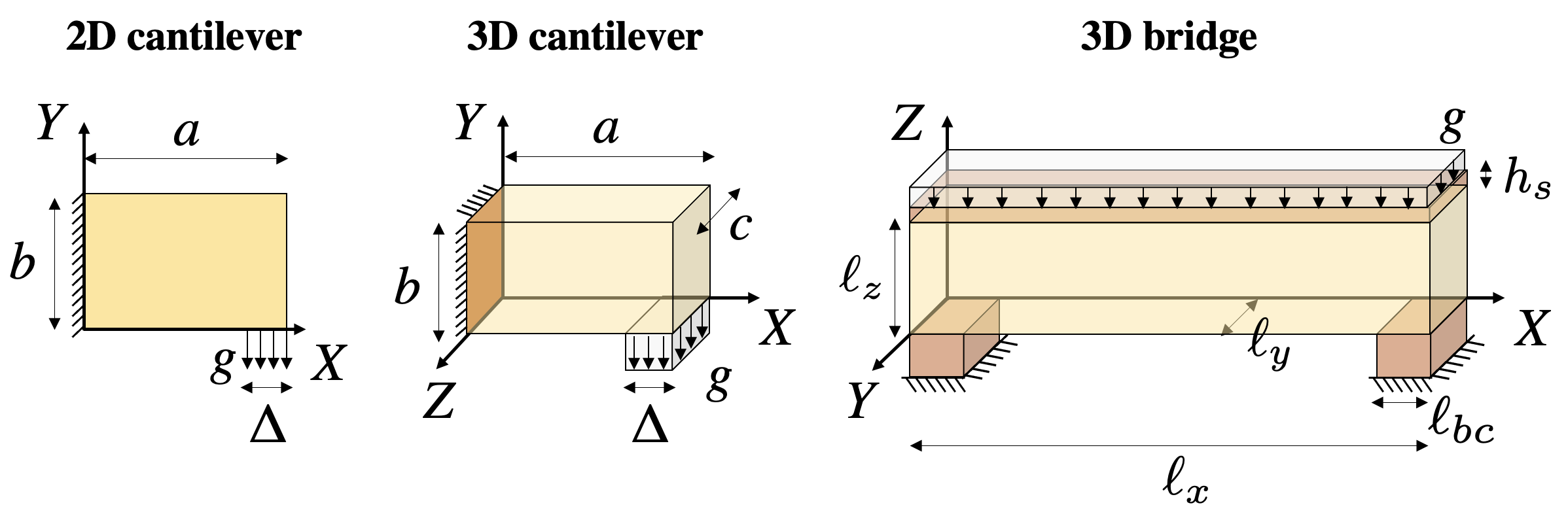
Figure 2: Design domain, loading and boundary conditions of numerical simulations: the 2D cantilever (Section 5.1); the 3D cantilever (Section 5.2); and the 3D bridge (Section 5.2).

5.1 2D simulations: parametric analyses

The 2D cantilever is solved starting from a two-dimensional design domain of rectangular shape with dimensions $a\times b$ (see Fig. 2), assuming plane strain conditions, with out-of-plane thickness $c$. The domain is clamped on the left vertical side and loaded by a downward vertically-oriented surface traction $g$ on a segment of length $\Delta$ at the right bottom end of the domain.

Table 1 reports geometrical and material parameters. If not differently specified, the initial conditions for the phase variable $\phi$ in the entire domain $\Omega$ are set as follows: $\phi_{0}=\mathrm{bar}{v}$ for all simulations relative to the formulation with volume constraint; $\phi_{0}=1$ for all simulations relative to the formulation with volume minimization. Colour maps of the phase-field variable $\phi$ are represented in the region of $\Omega$ where the phase variable $\phi\geq 0.1$. Moreover, the simulation time is normalized with respect to the time constant $T_{\phi}$ and, when not specified, a monolithic (SAND) solution strategy is adopted.

Parameter	$a$	$b$	$c$	$\Delta$	$g$	$E_{A}$	$\nu_{A}$	$\delta$	$p$
Unit	m	m	m	m	MPa	GPa	$-$	$-$	$-$
Value	2	1	1	0.2	500	10	0.25	$10^{-3}$	10

Table 1: Reference values of geometrical features, applied load, and material parameters of the 2D cantilever (Section 5.1).

Parameter	$\kappa_{\phi}$	$\gamma_{\phi}$	$\mathrm{bar}{v}$	$\kappa_{v}$	$\kappa_{b}$	$c_{AC}^{conv}$
Unit	MN/m	m	$-$	MPa	GPa	Pa s
Value	1	0.01	0.4	100	$10^{3}$	$10^{-6}$

Table 2: Reference values for simulation parameters adopted for the 2D cantilever (Section 5.1).

The design domain is discretized with $(120\times 60)$ square elements along the two coordinate axes. As a result of a preliminary convergence analysis, the employed mesh density allows to obtain mesh-independent results for all cases under investigation.

Table 2 reports the values of simulation parameters which are employed, if not object of a parametric investigation. It is noteworthy that adopted values respect the general rules-of-thumb traced in Section 4.1. In fact, the mesh size is $h_{e}=0.016$ m and $\mathrm{bar}{e}^{el}_{,\phi}=80$ MPa (with $g=500$ MPa). The target final volume fraction with the volume minimization functional hence results $v_{sol}^{tar}\approx 0.4$ with $\kappa_{v}=100$ MPa, that is comparable with the volume constraint value $\mathrm{bar}{v}=0.4$ assigned for the volume constraint functional.

5.1.1 Staggered (NAND) versus monolithic (SAND) solution strategy: convergence behaviour

The first set of analyses compares the convergence behaviour of a staggered (NAND) versus a monolithic (SAND) solution strategy. This comparison is made only with reference to the classical volume constraint approach, i.e., functional $\mathcal{L}_{AC}^{vc}$. Very similar results are however to be found for the novel volume minimization approach, i.e., functional $\mathcal{L}_{AC}^{vm}$, as well.

The evolution of the compliance $\mathcal{C}$ and of the Allen-Cahn error $\mathcal{E}_{AC}$ versus the simulation time is shown in Fig. 3(a). It can be observed that the error of the staggered approach decreases at the beginning of the simulation but starts to oscillate when reaching $\mathcal{E}_{AC}\approx 10^{-3}$, while the error of the monolithic strategy is substantially monotonic, down to the imposed value of $10^{-6}$.

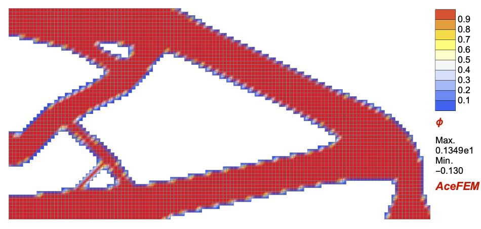
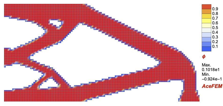
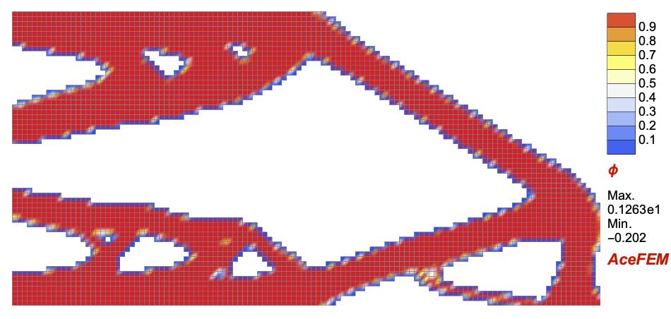
(b) Staggered approach (NAND)

Figure 5: Material distribution phase field $\phi_{sol}$ obtained with different values of the convergence parameter $c_{AC}^{conv}$ for the monolithic (a) and the staggered (b) solution approaches. Results are shown only with reference to the classical volume constraint approach (i.e., functional $\mathcal{L}_{AC}^{vc}$).

The obtained final solution is then investigated for different values of the convergence parameter $c_{AC}^{conv}$, value with respect to which convergence of the Allen-Cahn procedure is checked. Figure 3(b) reports the volume fraction $v_{sol}$ and the structural displacement $U_{sol}$ at the converged final solution, together with the final interface perimeter $\mathcal{P}_{sol}$. As previously noted, the staggered approach does not return a converged solution when enforcing $c_{AC}^{conv}\leq 10^{-3}$. The obtained solutions obviously coincide in terms of final volume fraction (since enforced by means of a global constraint), but not in terms of structural displacement and interface perimeter. A converged final value is not obtained with the staggered approach, while a converged solution is obtained with the monolithic one for $c_{AC}^{conv}\leq 10^{-3}$, although $c_{AC}^{conv}=10^{-2}$ would be practically sufficient. This outcome is confirmed by the maps on the distribution of the phase field variable at different values of $c_{AC}^{conv}$, reported in Fig. 5.

Finally, Figure 3(b) shows also the comparison on the total number of Newton-Raphson iterations, confirming the significant out-performance of the monolithic solution strategy (SAND) versus the staggered one (NAND). Therefore, all following analyses will adopt a monolithic (SAND) approach.

5.1.2 Volume constraint versus volume minimization: convergence behaviour

This section presents a comparison between the convergence behaviour of the volume constraint versus the volume minimization formulation. For both formulations, two different initial conditions are investigated, that is $\phi_{0}=1$ and $\phi_{0}=\mathrm{bar}{v}$ for $\mathcal{L}_{AC}^{vc}$, and $\phi_{0}=1$ and $\phi_{0}=0.5$ for $\mathcal{L}_{AC}^{vm}$.

Figure 6(a) shows the evolution of the volume fraction $v$ and of the compliance $\mathcal{C}$ along the simulation time. Contrarily to $\mathcal{L}_{AC}^{vc}$, the volume fraction $v$ with $\mathcal{L}_{AC}^{vm}$ evolves during the simulation, starting from the assigned initial condition. Structure compliance follows coherently. It is noteworthy that, for the chosen set of parameters, the final obtained solution between the two formulations is practically identical in terms of volume fraction and compliance, making the comparison consistent.

Figure 6(a) reports also the Allen-Cahn convergence error $\mathcal{E}_{AC}$ along the simulation time. In all cases, results show an acceptable convergence behaviour, with a similar decrease rate of $\mathcal{E}_{AC}$ between the two formulations. However, the evolution of $\mathcal{E}_{AC}$ for the volume constraint functional $\mathcal{L}_{AC}^{vc}$ is significantly more oscillatory than the one obtained for the volume minimization one $\mathcal{L}_{AC}^{vm}$.

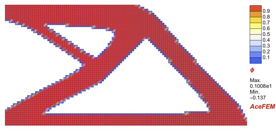
$c_{AC}^{conv}=10^{-4}$

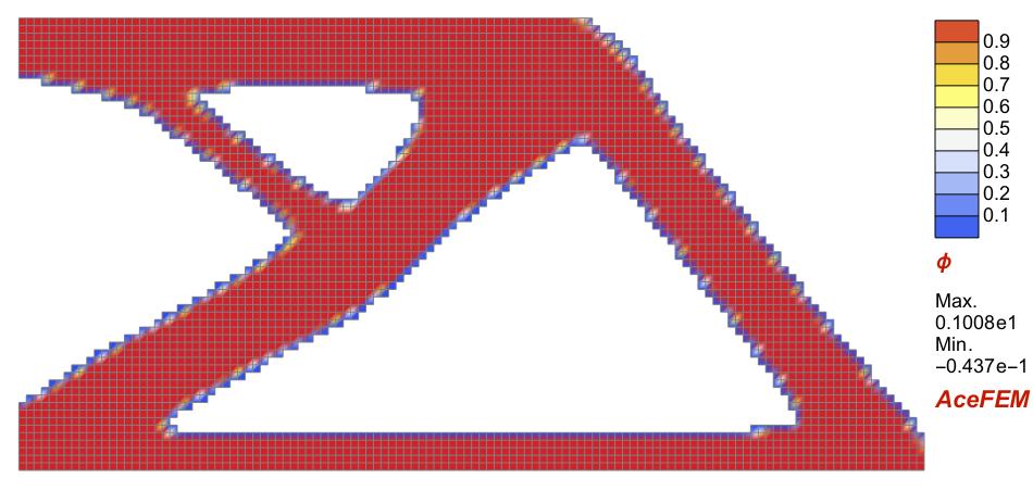
$c_{AC}^{conv}=10^{-2}$

(a) Volume constraint $\mathcal{L}_{AC}^{vc}$ $-$ $\text{I.C.}:\phi_{0}=1$ and $\phi_{0}=\mathrm{bar}{v}$

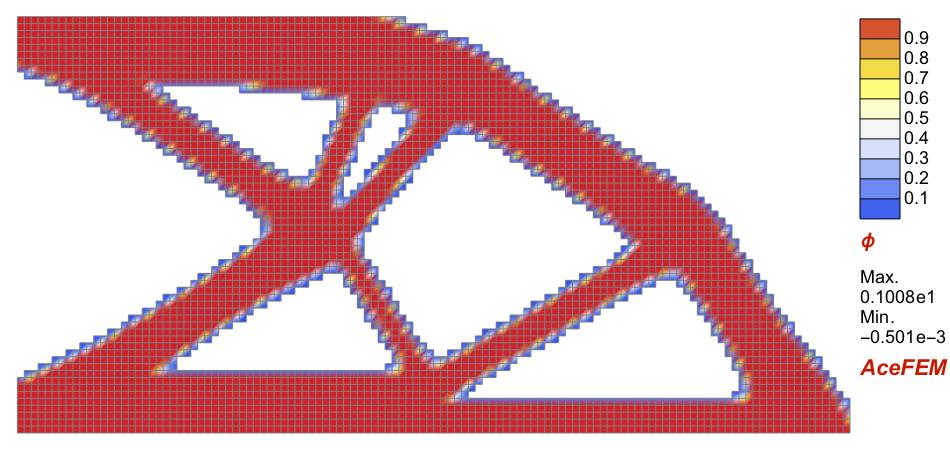
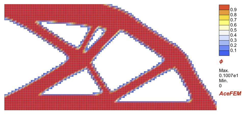
(b) Volume minimization $\mathcal{L}_{AC}^{vm}$ $-$ $\text{I.C.}:\phi_{0}=1$

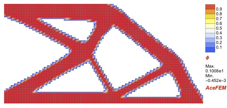
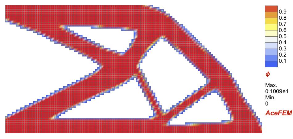
(c) Volume minimization $\mathcal{L}_{AC}^{vm}$ $-$ $\text{I.C.}:\phi_{0}=0.5$

Figure 8: Material distribution phase field $\phi_{sol}$ obtained with different values of the convergence parameter $c_{AC}^{conv}$ and different initial conditions (I.C.) for: a) the volume constraint formulation (coinciding with $\phi_{0}=\mathrm{bar}{v}$ and $\phi_{0}=1$); b) the volume minimization formulation with $\phi_{0}=1$; c) the volume minimization formulation with $\phi_{0}=0.5$.

The final solution is then investigated for different values of the convergence parameter $c_{AC}^{conv}$ (with respect to which convergence of the Allen-Cahn procedure is checked). The final values of $v_{sol}$ and $U_{sol}$ are reported in Fig. 6(b), together with $\mathcal{P}_{sol}$. Below a given threshold (ca. $10^{-2}-10^{-4}$), both formulations show a robust and converged solution. This outcome is confirmed by the maps on the distribution of the phase field variable at different values of $c_{AC}^{conv}$, reported in Fig. 8.

Moreover, Fig. 6(b) reports the number of Newton-Raphson iterations required for the solution, clearly proving the computational out-performance of the volume minimization approach $\mathcal{L}_{AC}^{vm}$ with respect to the volume constraint one $\mathcal{L}_{AC}^{vc}$.

The effect of the initial condition for the volume constraint functional $\mathcal{L}_{AC}^{vc}$ is negligible both in terms of final solution and numerical performances. This is due to the fact that, at the very first step, the global constraint changes the value of $\phi$ from $\phi_{0}$ to $\mathrm{bar}{v}$. On the other hand, for the volume minimization functional $\mathcal{L}_{AC}^{vm}$, the choice on $\phi_{0}$ affects the solution. In fact, only minor differences are obtained in terms of final obtained solution (see also Fig. 8), but the convergence behaviour is significantly different, $\phi_{0}=1$ requiring a significantly lower number of Newton-Raphson iterations than $\phi_{0}=0.5$. This is also observable in Fig. 6(a) by noting that the adaptive solution scheme with $\phi_{0}=0.5$ significantly reduces the reference time-step increment $\delta t_{0}=10^{-2}$, while $\phi_{0}=1$ not. Accordingly, in what follows, the initial condition $\phi_{0}=1$ will be adopted for the volume minimization functional $\mathcal{L}_{AC}^{vm}$, while $\phi_{0}=\mathrm{bar}{v}$ for $\mathcal{L}_{AC}^{vc}$.

5.1.3 Volume constraint versus volume minimization: amount of distributed material

This section analyzes the two formulations by varying the amount of distributed material. This is achieved by varying $\mathrm{bar}{v}$ for the volume constraint functional $\mathcal{L}_{AC}^{vc}$, and $\kappa_{v}$ for the volume minimization functional $\mathcal{L}_{AC}^{vm}$. For the latter, the value of the perimeter stiffness parameter $\kappa_{\phi}$ varies with $\kappa_{v}$ according to the relationship $\kappa_{\phi}=\gamma_{\phi}\kappa_{v}$, as described in Section 4.1.

As shown in Fig. 9, for $\mathcal{L}_{AC}^{vc}$, the assigned value $\mathrm{bar}{v}$ clearly corresponds to the obtained final volume fraction $v_{sol}$ for the entire range of the parametric analysis, verifying the correctness of the implementation of the global constraint. On the other hand, for $\mathcal{L}_{AC}^{vc}$, the relationship between $\kappa_{v}$ and $v_{sol}$ is non-linear. Remarkably, the obtained trend is very-well captured by the theoretical target estimate $v_{sol}^{tar}(\kappa_{v})$ provided in Eq. (4.52).

Figure 10 shows that, for a given value of final volume fraction $v_{sol}$, the solutions obtained from the two formulations are practically identical in terms of structural displacement $U_{sol}$, as well as maximum $\sigma_{vm}^{max}$ and average $\sigma_{vm}^{avg}$ Von-Mises stresses. The effective distribution of the phase-field variable is also very similar, although differences are observable in Fig. 12 and again in Fig. 10 as regards the interface perimeter $\mathcal{P}_{sol}$.

Finally, the analysis of the performance of the two formulations (in terms of Newton-Raphson iterations, see Fig. 10) show that the volume minimization functional $\mathcal{L}_{AC}^{vm}$ is significantly more efficient ($>50\%$ iteration saving) than $\mathcal{L}_{AC}^{vc}$ for the more challenging cases cases where the final volume fraction is low, that is $v_{sol}<0.5$, cases which are also more interesting from the engineering viewpoint.

5.1.4 Volume constraint versus volume minimization: effect of load variations

The last comparison between the two formulations addresses the effect of the applied load magnitude $g$ on the final solution. In this case, the volume constraint $\mathrm{bar}{v}$ (for $\mathcal{L}_{AC}^{vc}$) and the volume penalty $\kappa_{v}$ (for $\mathcal{L}_{AC}^{vm}$) are held constant, as given in Table 2.

Figure 13 clearly show the difference on the rationale upon which the two functionals are built. In fact, the load magnitude $g$ highly affects the final obtained structural displacement $U_{sol}$ when employing a volume constrained principle (i.e., $\mathcal{L}_{AC}^{vc}$) because the final volume fraction $v_{sol}$ is assigned a priori. This is accompanied by high variations in stresses, while the final design is practically independent from the load (see Fig. 15). On the other hand, the load magnitude $g$ highly affects the final volume fraction $v_{sol}$ obtained when employing a volume minimization principle (i.e., $\mathcal{L}_{AC}^{vm}$). At different load levels, final designs associated with similar values of structural displacement $U_{sol}$ and stresses $\sigma_{vm}^{max}$ and $\sigma_{vm}^{avg}$ are obtained. As shown in Fig. 15, the obtained design with $\mathcal{L}_{AC}^{vm}$ is now highly affected by the applied load value $g$.

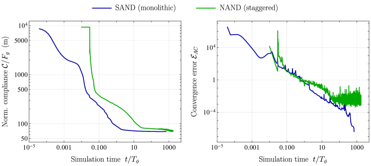
(a) Compliance $\mathcal{C}(\phi,{\bf u})$ (left) and Allen-Cahn error $\mathcal{E}_{AC}$ (right).

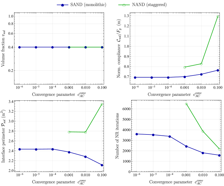
(b) Volume fraction $v_{sol}$ (top left), normalized compliance $\mathcal{C}_{sol}/F_{g}$ (top right), interface perimeter $\mathcal{P}_{sol}$ (bottom left), and total number of Newton-Raphson iterations (bottom right).

Figure 3: Convergence behaviour of a staggered (SAND) and a monolithic solution (NAND) strategy: a) evolution of the computed solution versus the simulation time $t/T_{\phi}$; b) effect of the convergence parameter $c_{AC}^{conv}$ on the final computed solution. Results are shown only with reference to the classical volume constraint approach (i.e., functional $\mathcal{L}_{AC}^{vc}$).

$c_{AC}^{conv}=10^{-3}$

$c_{AC}^{conv}=10^{-2}$

$c_{AC}^{conv}=10^{-1}$

(a) Monolithic approach (SAND)

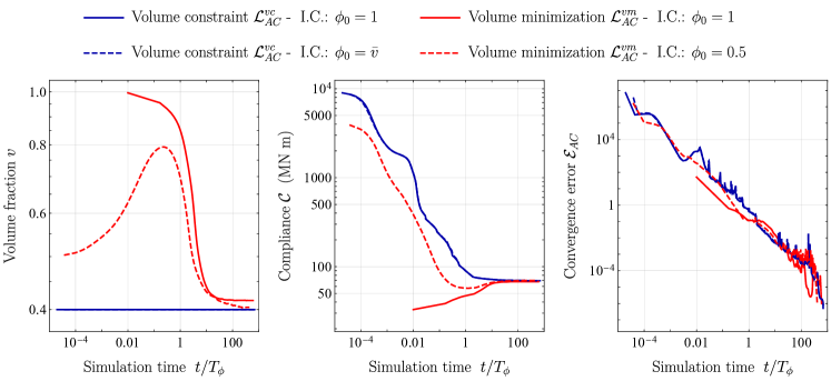
(a) Volume fraction $v(\phi)$ (left), compliance $\mathcal{C}(\phi,{\bf u})$ (center) and Allen-Cahn error $\mathcal{E}_{AC}$ (right).

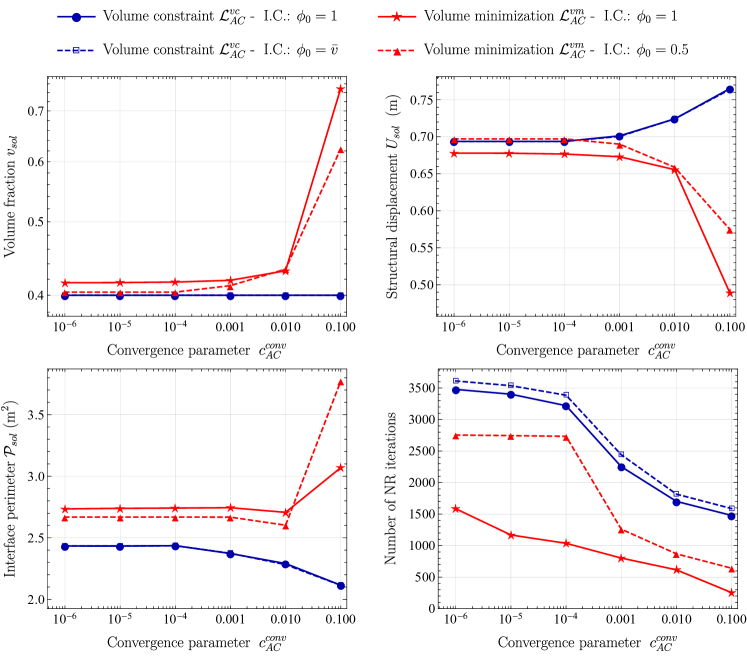
(b) Volume fraction $v_{sol}$ (top left), structural displacement $U_{sol}$ (top right), interface perimeter $\mathcal{P}_{sol}$ (bottom left), and total number of Newton-Raphson iterations (bottom right).

Figure 6: Convergence behaviour of the two formulations with different initial conditions: a) evolution of the computed solution versus the simulation time $t/T_{\phi}$; b) effect of the convergence parameter $c_{AC}^{conv}$ on the final computed solution.

$c_{AC}^{conv}=10^{-6}$

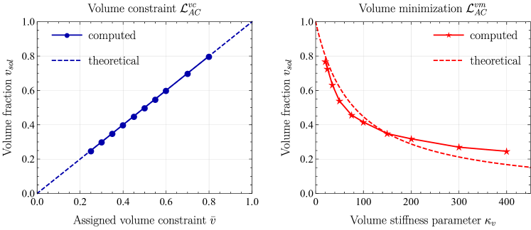
Figure 9: Parametric study on the amount of distributed material with the volume constraint and the volume minimization functionals. Total volume fraction $v_{sol}$ obtained by varying the assigned volume constraint parameter $\mathrm{bar}{v}$ in $\mathcal{L}_{AC}^{vc}$ (left), and by varying the volume penalty parameter $\kappa_{v}$ (with $\kappa_{\phi}=\gamma_{\phi}\kappa_{v}$) in $\mathcal{L}_{AC}^{vm}$ (right). Computed values are compared with the estimated theoretical values $v_{sol}=\mathrm{bar}{v}$ for $\mathcal{L}_{AC}^{vc}$ and $v_{sol}=v_{sol}^{tar}(\kappa_{v})$ in Eq. (4.52) for $\mathcal{L}_{AC}^{vm}$.

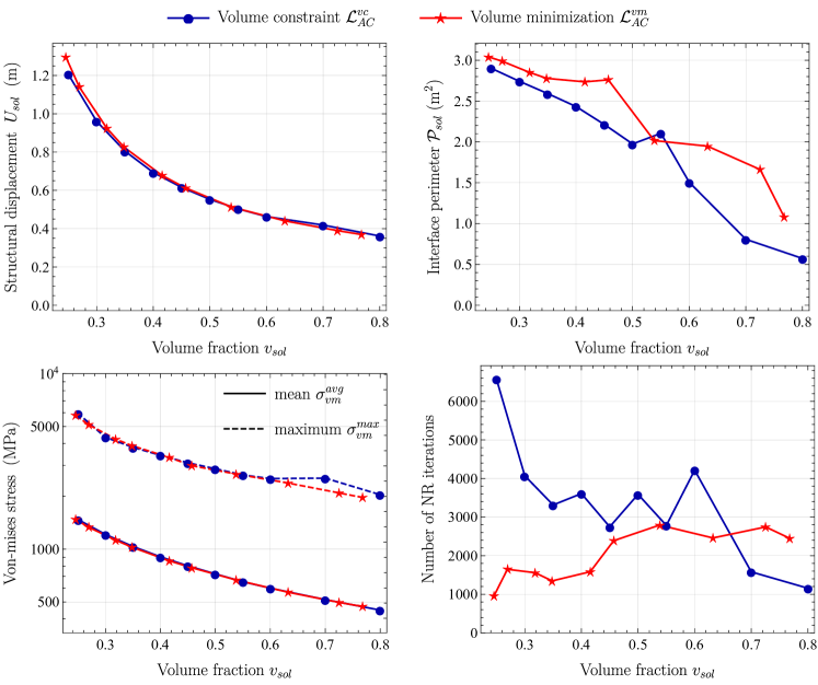
Figure 10: Parametric study on the amount of distributed material with the volume constraint and the volume minimization functional. Structural displacement $U_{sol}$ (top left), interface perimeter $\mathcal{P}_{sol}$ (top right), maximum $\sigma_{vm}^{max}$ and average $\sigma_{vm}^{avg}$ Von-Mises stresses (bottom left), and total number of Newton-Raphson iterations (bottom right) versus the obtained total volume fraction $v_{sol}$.

$\mathrm{bar}{v}=0.25$

$\mathrm{bar}{v}=0.40$

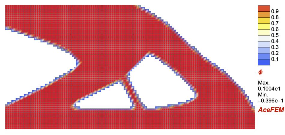
$\mathrm{bar}{v}=0.60$

(a) Volume constraint $\mathcal{L}_{AC}^{vc}$

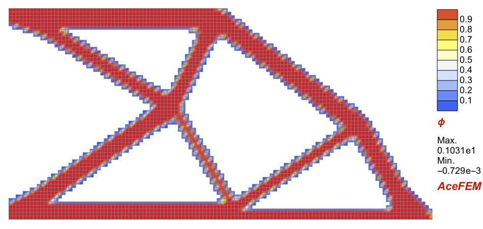
$\kappa_{v}=300$ MPa, $v_{sol}\approx 0.25$

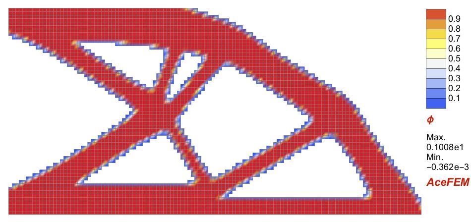
$\kappa_{v}=100$ MPa, $v_{sol}\approx 0.4$

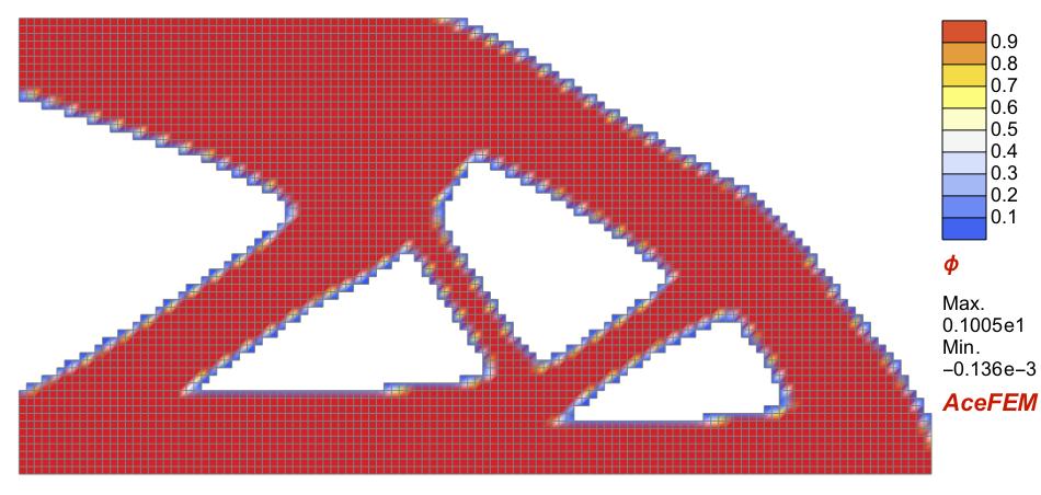
$\kappa_{v}=50$ MPa, $v_{sol}\approx 0.6$

(b) Volume minimization $\mathcal{L}_{AC}^{vm}$

Figure 12: Material distribution phase field $\phi_{sol}$ obtained with different values of obtained by varying the assigned volume constraint parameter $\mathrm{bar}{v}$ in $\mathcal{L}_{AC}^{vc}$ (a), and by varying the volume penalty parameter $\kappa_{v}$ (with $\kappa_{\phi}=\gamma_{\phi}\kappa_{v}$) in $\mathcal{L}_{AC}^{vm}$ (b).

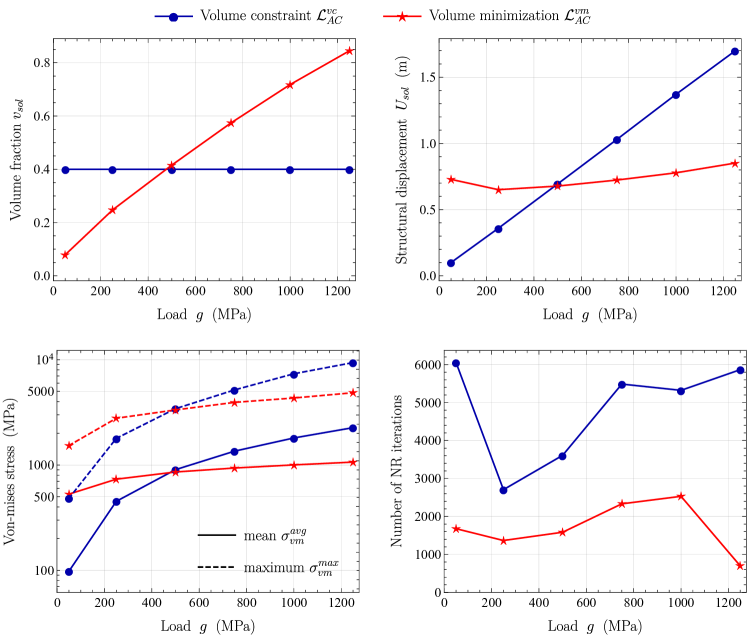
Figure 13: Parametric study on the applied load with the volume constraint ($\mathrm{bar}{v}=0.4$) and the volume minimization ($\kappa_{v}=100$ MPa) functionals. Total volume fraction $v_{sol}$ (top left), structural displacement $U_{sol}$ (top right), maximum $\sigma_{vm}^{max}$ and average $\sigma_{vm}^{avg}$ Von-Mises stresses (bottom left), and total number of Newton-Raphson iterations (bottom right) versus the applied load magnitude $g$.

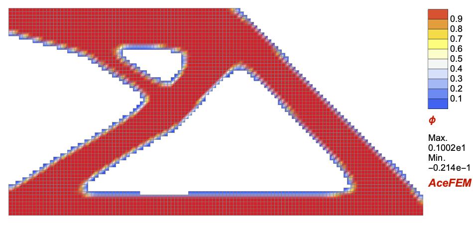
$g=250$ MPa

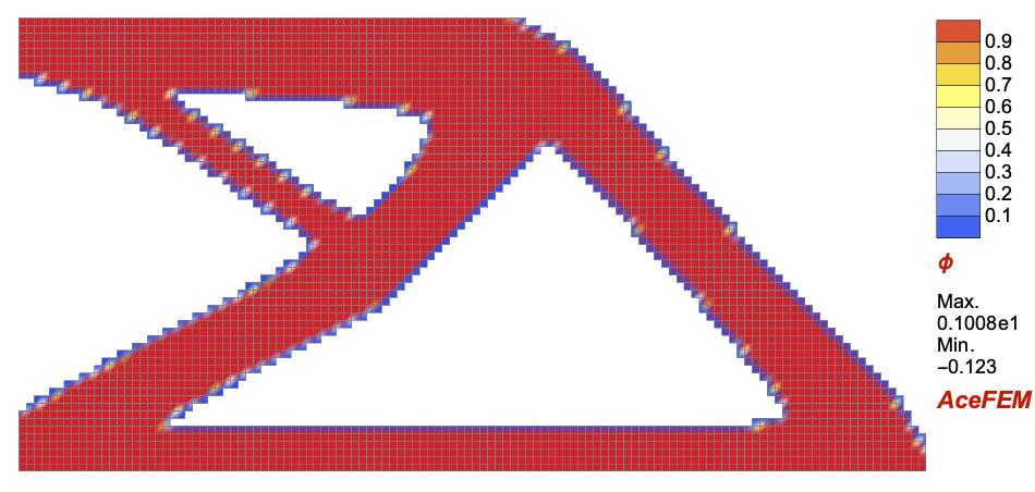
$g=500$ MPa

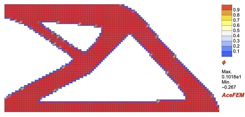
$g=750$ MPa

(a) Volume constraint $\mathcal{L}_{AC}^{vc}$

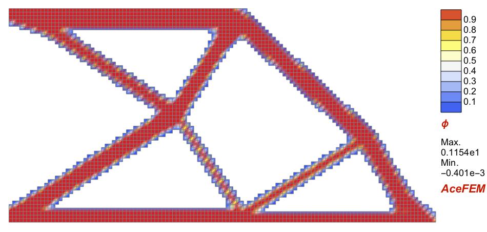
(b) Volume minimization $\mathcal{L}_{AC}^{vm}$

Figure 15: Material distribution phase field $\phi_{sol}$ obtained with different values of the applied load magnitude $g$ for: a) the volume constraint formulation with $\mathrm{bar}{v}=0.4$; b) the volume minimization formulation with $\kappa_{v}=100$ MPa.

5.2 3D simulations

In this section, the novel volume minimization functional $\mathcal{L}_{AC}^{vm}$ is tested on two 3D problems. In particular, the addressed examples are (see Fig. 2):

• A cantilever beam, representing the 3D counterpart of the case study presented in Section 5.1. The domain is now discretized by means of $80\times 40\times 40$ hexahedral elements, resulting in an average element size $h_{e}=0.025$ m. The geometrical and material features, as well as the applied load magnitude, correspond to the values listed in Table 1, while values of simulation parameters to the ones in Table 2 apart from $\gamma_{\phi}=0.02$ m (due to a slight increase in the dimension of the elements in the mesh), and $c_{AC}^{conv}=10^{-2}$ (fixed on the basis of the convergence analysis in Section 5.1.2);

• A bridge, as the one investigated in Zegard and Paulino (2016). The design domain is represented by a rectangular cuboid $\ell_{x}\times\ell_{y}\times\ell_{z}$. The domain is fixed on the bottom plane at $Z=0$ along strips of length $l_{bc}$ along $X$. Moreover, a passive solid slab on the top surface at $Z=\ell_{z}$ of height $h_{s}$ m is considered, on top of which a distributed load $g$ is applied in the $Z$-direction. Material properties correspond to the one of the previous example, being reported in Table 1. Values of geometrical and simulation parameters, as well as load magnitude, are given in Table 3. The domain is discretized by means of $150\times 30\times 30$ hexahedral elements, resulting in an average element size $h_{e}\approx 0.3$ m.

Parameter	$\ell_{x}$	$\ell_{y}$	$\ell_{z}$	$\ell_{bc}$	$h_{s}$	$g$	$\kappa_{\phi}$	$\gamma_{\phi}$	$\kappa_{v}$	$c_{AC}^{conv}$
Unit	m	m	m	m	m	MPa	MN/m	m	MPa	$-$
Value	44	8.8	8.8	1.76	0.2	150	200	0.2	1000	$10^{-2}$

Table 3: Values of geometrical and simulation parameters employed in the 3D bridge case study. Only values different from the ones in Tables 1 and 2 are reported.

In particular, the 3D cantilever has been addressed to show that the proposed formulation can be straightforwardly implemented in a 3D computational framework, analyzing differences obtained from a 2D to a 3D setting for the same case study. The bridge is instead defined such to have significant differences in the physical dimension of the problem, in order to prove the robustness of the parameter settings guidelines traced in Section 4.1, with particular reference to $\kappa_{v}$, $\gamma_{\phi}$, and $\kappa_{\phi}$.

Since the volume minimization functional is adopted, the setting of the volume penalty parameter plays a fundamental role. For the cantilever, we have $\mathrm{bar}{e}^{el}_{\phi}=84$ MPa and hence $v_{sol}^{tar}\approx 0.4$ with $\kappa_{v}=100$ MPa; for the bridge, we have $\mathrm{bar}{e}^{el}_{\phi}=170$ MPa and hence $v_{sol}^{tar}\approx 0.2$ with $\kappa_{v}=1000$ MPa. Figure 16 shows the comparison between the estimated and final obtained volume fractions, confirming the effectiveness of the proposed procedure for obtaining the target solution.

The final obtained designs are shown in Fig. 17 for the cantilever, and in Fig. 18 for the bridge. Three-dimensional patterns clearly arise, with regular external and internal surfaces obtained without the need of post-processing filtering techniques thanks to the adopted phase-field rationale.

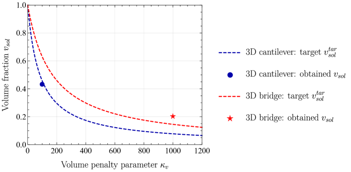
Figure 16: 3D applications: estimated target volume fractions $v_{sol}^{tar}$ versus obtained volume fraction $v_{sol}$.

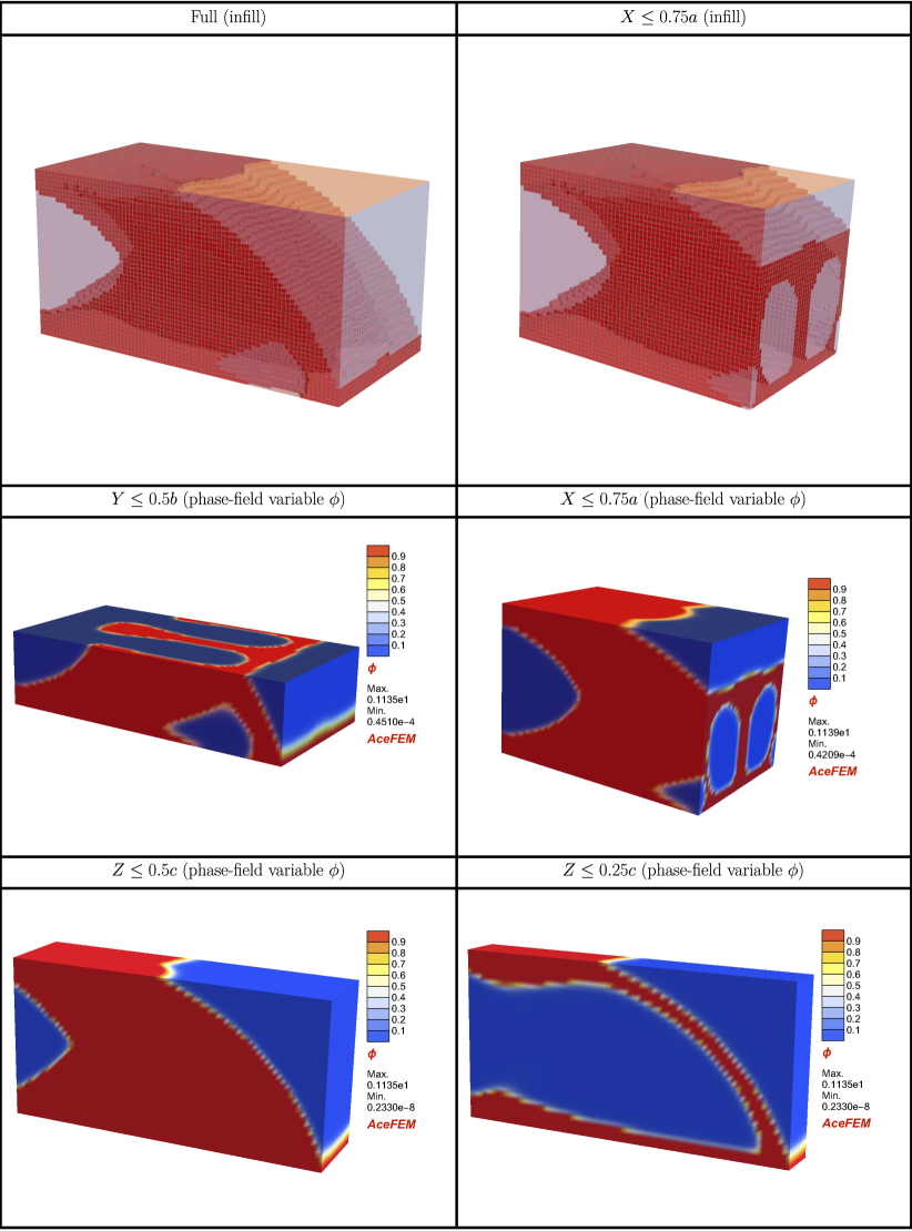
Figure 17: Topology optimization of the 3D cantilever.

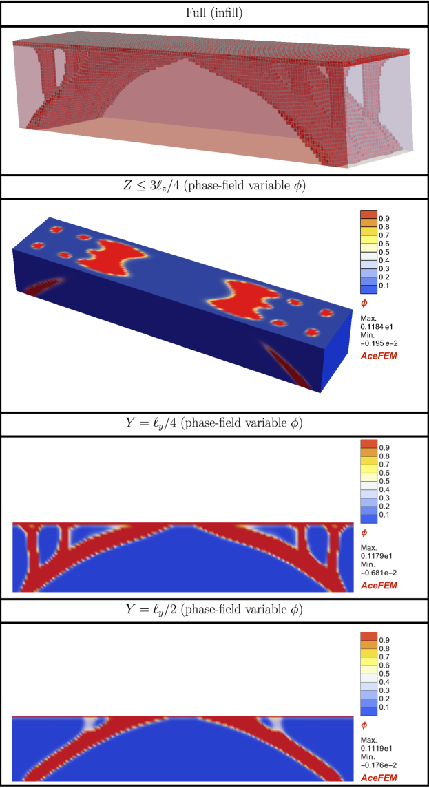
Figure 18: Topology optimization of the 3D bridge.

6 Comparison between investigated formulations and conclusions

The present work addresses a rigorous study on basic properties of structural topology optimization problems with phase-field. In particular, we performed the following five tasks:

1. Proposed mixed Hu-Washizu variational formulations for the topology optimization problem with phase-field to directly impose equilibrium, constitutive, and compatibility equations in the formulation;

2. Investigated two different topology optimization principles, e.g.,: i) a formulation imposing a priori the amount of material to be distributed within the design domain (formulation with volume constraint); ii) a formulation based on a minimization of material to be distributed, given that a cost (i.e., a penalty parameter) is assigned to the material (formulation with volume minimization);

3. Introduced a Simultaneous Analysis and Design (SAND) monolithic solution strategy, thanks to the Hu-Washizu functional rationale and based on an Allen-Cahn scheme, where the phase-field variable evolves under the respect of mechanical equilibrium at each computational incremental step;

4. Analyzed both numerical convergence behaviours and obtained final designs, based on comparative analyses between simulation strategies (monolithic SAND vs. staggered NAND) and between topology optimization principles (volume constraint vs. minimization);

5. Analyzed the performance of the proposed variational formulation based on volume minimization also on three-dimensional case studies.

On the basis of theoretical considerations, general guidelines are traced for properly setting the value of simulation parameters characterizing the phase-field evolution (i.e., $\tau_{\phi}$, $\kappa_{\phi}$ and $\gamma_{\phi}$). Following this careful setting, the implemented finite element formulations and solution algorithm are robust, allowing to conduct a wide campaign of parametric simulations without encountering any numerical convergence issue. In addition, the volume penalty parameter $\kappa_{v}$ in the volume minimization functional has been related to target values of volume fraction.

From the obtained results, we may conclude the following:

• A monolithic SAND solution strategy significantly outperforms a staggered NAND solution strategy (see Fig. 3);

• The volume minimization formulation $\mathcal{L}^{vm}$ shows an Allen-Cahn convergence behavior with better properties than the volume constraint formulation $\mathcal{L}^{vc}$, since the decrease of the Allen-Cahn error measure $\mathcal{E}_{AC}$ is highly oscillatory for $\mathcal{L}^{vc}$ but not for $\mathcal{L}^{vm}$ (see Fig. 6);

• Comparing designs with the same final volume fraction $v_{sol}$, the two formulations lead to practically coincident solutions in terms of compliance $\mathcal{C}_{sol}$ (or structural displacement $U_{sol}$) and interface perimeter $\mathcal{P}_{sol}$ (see Fig. 10), although final designs are slightly different (see Fig. 12);

• The final design is practically independent from the applied load with the volume constraint functional $\mathcal{L}^{vc}$, while is highly affected with the volume minimization one $\mathcal{L}^{vm}$ (see Figs. 13 and 15), which is seen as a significative advantage of this latter formulation;

• The number of Newton-Raphson iterations required for solving the problem with the the volume minimization functional $\mathcal{L}^{vm}$ is in most cases significantly lower (less than $50\%$) than the ones employed with the volume constraint functional $\mathcal{L}^{vc}$;

• No convergence issues are encountered in 3D applications (see Figs. 17 and 18), allowing to obtain (thanks to the phase-field rationale) complex but regular patterns without the need of any post-processing filtering technique (as required by density-based approaches) which might lead to undesirable (artificial) effects (Zegard and Paulino, 2016).

In conclusion, the obtained results highlight fundamental aspects of structural topology optimization problems with phase-field, allowing to optimize the solution strategy and to trace guidelines for settings simulation parameters beforehand. Referring in particular to the proposed volume minimization principle, we believe that these results can be a starting point for more advanced developments of phase-field topology optimization that considers loading uncertainties (Dunning et al., 2011) or multi-target strategies, e.g., controlling both geometry and compliance (Strömberg, 2010), both geometry and stresses (Burger and Stainko, 2006), the structure life-cycle cost (Sarma and Adeli, 2002), or manufacturing costs (Liu et al., 2019).

Conflict of interest

The authors declare that they have no conflict of interest.

Replication of Results

The paper already contains all the data necessary to properly replicate all the presented results.

Appendix A Interpolation of the stress and strain fields

The interpolation matrices of the stress and strain fields employed for 2D and 3D applications are detailed in what follows. Choices follow arguments presented in Weisman (1996), Cao et al. (2002) and Djoko et al. (2006). In detail, minimum distributions required for stability are included as a common basis between the assumed stress and strain fields. In addition, the assumed strain field is enriched with respect to the stress one with strain modes not already contained in the minimum one. A minimal strain enrichment, a priori orthogonal to the assumed stress field, is considered. Interesting extensions of the present work would be to investigate more refined enrichment strategies, accompanied by a generalization of the introduced mixed formulations, in order to deal with material constrained behaviours (e.g., incompressibility or inextensibility).

A.1 2D applications

The stress field $\boldsymbol{\sigma}$ is approximated in a discontinuous element-by-element form, introducing five element unknowns collected in vector $\hat{\boldsymbol{\sigma}}=(\hat{\sigma}_{1},\ldots,\hat{\sigma}_{5})$ and the following definition of $\boldsymbol{N}_{\boldsymbol{\sigma}}(\boldsymbol{\xi})$:

$$\text{vec}(\boldsymbol{\sigma}_{\boldsymbol{\xi}})=\left(\begin{array}[]{c}\sigma_{\xi\xi}\\ \sigma_{\eta\eta}\\ \sigma_{\xi\eta}\end{array}\right)=\boldsymbol{N}_{\boldsymbol{\sigma}}(\boldsymbol{\xi})\hat{\boldsymbol{\sigma}}\hskip 8.53581pt\text{with}\hskip 8.53581pt\boldsymbol{N}_{\boldsymbol{\sigma}}(\boldsymbol{\xi})=\left[\begin{array}[]{ccccccc}1&\eta&0&0&0\\ 0&0&1&\xi&0\\ 0&0&0&0&1\end{array}\right]\,.$$ (A.1)

The strain field $\boldsymbol{\varepsilon}$ is approximated in a discontinuous element-by-element form, introducing seven element unknowns collected in vector $\hat{\boldsymbol{\varepsilon}}=(\hat{\epsilon}_{1},\ldots,\hat{\epsilon}_{7})$ and the following definition of $\boldsymbol{N}_{\boldsymbol{\varepsilon}}(\boldsymbol{\xi})$

$$\text{vec}(\boldsymbol{\varepsilon}_{\boldsymbol{\xi}})=\left(\begin{array}[]{c}\epsilon_{\xi\xi}\\ \epsilon_{\eta\eta}\\ 2\epsilon_{\xi\eta}\end{array}\right)=\boldsymbol{N}_{\boldsymbol{\varepsilon}}(\boldsymbol{\xi})\hat{\boldsymbol{\varepsilon}}\hskip 8.53581pt\text{with}\hskip 8.53581pt\boldsymbol{N}_{\boldsymbol{\varepsilon}}(\boldsymbol{\xi})=\left[\begin{array}[]{ccccccc}1&\xi&\eta&0&0&0&0\\ 0&0&0&1&\xi&\eta&0\\ 0&0&0&0&0&0&1\end{array}\right]\,.$$ (A.2)

A.2 3D applications

The stress field $\boldsymbol{\sigma}$ is approximated in a discontinuous element-by-element form, introducing eighteen element unknowns collected in vector $\hat{\boldsymbol{\sigma}}=(\hat{\sigma}_{1},\ldots,\hat{\sigma}_{18})$ and the following definition of $\boldsymbol{N}_{\boldsymbol{\sigma}}(\boldsymbol{\xi})$:

$$\text{vec}(\boldsymbol{\sigma}_{\boldsymbol{\xi}})=\left(\begin{array}[]{c}\sigma_{\xi\xi}\\ \sigma_{\eta\eta}\\ \sigma_{\zeta\zeta}\\ \sigma_{\eta\zeta}\\ \sigma_{\xi\zeta}\\ \sigma_{\xi\eta}\end{array}\right)=\boldsymbol{N}_{\boldsymbol{\sigma}}(\boldsymbol{\xi})\hat{\boldsymbol{\sigma}}\hskip 8.53581pt\text{with}\hskip 8.53581pt\boldsymbol{N}_{\boldsymbol{\sigma}}(\boldsymbol{\xi})=\left[\begin{array}[]{cccccccccccccccccc}1&\eta&\zeta&\eta\zeta&0&0&0&0&0&0&0&0&0&0&0&0&0&0\\ 0&0&0&0&1&\xi&\zeta&\xi\zeta&0&0&0&0&0&0&0&0&0&0\\ 0&0&0&0&0&0&0&0&1&\xi&\eta&\xi\eta&0&0&0&0&0&0\\ 0&0&0&0&0&0&0&0&0&0&0&0&1&\xi&0&0&0&0\\ 0&0&0&0&0&0&0&0&0&0&0&0&0&0&1&\eta&0&0\\ 0&0&0&0&0&0&0&0&0&0&0&0&0&0&0&0&1&\zeta\end{array}\right]\,.$$ (A.3)

The strain field $\boldsymbol{\varepsilon}$ is approximated in a discontinuous element-by-element form, introducing twenty-one element unknowns collected in vector $\hat{\boldsymbol{\varepsilon}}=(\hat{\epsilon}_{1},\ldots,\hat{\epsilon}_{21})$ and the following definition of $\boldsymbol{N}_{\boldsymbol{\varepsilon}}(\boldsymbol{\xi})$

$$\text{vec}(\boldsymbol{\varepsilon}_{\boldsymbol{\xi}})=\left(\begin{array}[]{c}\epsilon_{\xi\xi}\\ \epsilon_{\eta\eta}\\ \epsilon_{\zeta\zeta}\\ 2\epsilon_{\eta\zeta}\\ 2\epsilon_{\xi\zeta}\\ 2\epsilon_{\xi\eta}\end{array}\right)=\boldsymbol{N}_{\boldsymbol{\sigma}}(\boldsymbol{\xi})\hat{\boldsymbol{\sigma}}\hskip 8.53581pt\text{with}\hskip 8.53581pt\boldsymbol{N}_{\boldsymbol{\varepsilon}}(\boldsymbol{\xi})=\left[\begin{array}[]{ccccccccccccccccccccc}1&\xi&\eta&\zeta&\eta\zeta&0&0&0&0&0&0&0&0&0&0&0&0&0&0&0&0\\ 0&0&0&0&0&1&\xi&\eta&\zeta&\xi\zeta&0&0&0&0&0&0&0&0&0&0&0\\ 0&0&0&0&0&0&0&0&0&0&1&\xi&\eta&\zeta&\xi\eta&0&0&0&0&0&0\\ 0&0&0&0&0&0&0&0&0&0&0&0&0&0&0&1&\xi&0&0&0&0\\ 0&0&0&0&0&0&0&0&0&0&0&0&0&0&0&0&0&1&\eta&0&0\\ 0&0&0&0&0&0&0&0&0&0&0&0&0&0&0&0&0&0&0&1&\zeta\end{array}\right]\,.$$ (A.4)

References

- Allaire et al. (2004) Allaire, G., Jouve, F., Maillot, H., 2004. Topology optimization and optimal shape design using homogenization. Struct. Multidisc. Optim. 28, 87–98.
- Auricchio et al. (2019) Auricchio, F., Bonetti, E., Carraturo, M., Hömberg, D., Reali, A., E., R., 2019. A phase-field based on graded-material topology optimization with stress constraint. arXiv:1907.06355, Math. Models Meth. Appl. Sci., to appear.
- Bendsøe (1983) Bendsøe, M. P., 1983. On obtaining a solution to optimization problems for solid, elastic plates by restriction of the design space. J. Struct. Mech. 11 (4), 501–521.
- Bendsøe and Sigmund (1999) Bendsøe, M. P., Sigmund, O., 1999. Material interpolation schemes in topology optimization. Archive of Applied Mechanics 6 65, 635–654.
- Blank et al. (2014a) Blank, L., Farshbaf-Shaker, M., Garcke, H., Rupprecht, C., Styles, V., 2014a. Multi-material Phase Field Approach to Structural Topology Optimization. In: Leugering, G., Benner, P., Engell, S., Griewank, S., Harbrecht, H., Hinze, M., Rannacher, R., Ulbrich, S. (Eds.), Trends in PDE Constrained Optimization. Vol. 165. Springer International Publishing, Cham, pp. 231–246.
- Blank et al. (2014b) Blank, L., Garcke, H., Farshbaf-Shaker, M., V., S., 2014b. Relating phase field and sharp interface approaches to structural topology optimization. ESAIM Control Optim. Calc. Var. 20, 1025–1058.
- Bourdin and Chambolle (2003) Bourdin, B., Chambolle, A., 2003. Design-dependent loads in topology optimization. ESAIM Contr. Optim. Calc. Var. 9, 19–48.
- Burger (2003) Burger, M., 2003. A framework for the construction of level set methods for shape optimization and reconstruction. Interfaces Free Bound. 5, 301–332.
- Burger and Stainko (2006) Burger, M., Stainko, R., 2006. Phase-field relaxation of topology optimization with local stress constraints. SIAM J. Control Optim. 45 (4), 1447–1466.
- Cao et al. (2002) Cao, Y. P., Hu, N., Lu, J., Fukunaga, H., Yao, Z. H., 2002. A 3D brick element based on Hu-Washizu variational principle for mesh distortion. Internat. J. Numer. Methods Engrg. 53 (11), 2529–2548.
- Carraturo et al. (2019) Carraturo, M., Rocca, E., Bonetti, E., Hömberg, D., Reali, A., F., A., 2019. Graded-material Design based on Phase-field and Topology Optimization. Computational Mechanics, DOI: 10.1007/s00466–019–01736–w.
- Deaton and Grandhi (2014) Deaton, J. D., Grandhi, R. V., 2014. A survey of structural and multidisciplinary continuum topology optimization: post 2000. Structural and Multidisciplinary Optimization 49 (1), 1–38.
- Dedè et al. (2012) Dedè, L., Borden, M. J., Hughes, T. J., 2012. Isogeometric analysis for topology optimization with a phase field model. Archives of Computational Methods in Engineering 19 (3), 427–465.
- Djoko et al. (2006) Djoko, J., Lamichhane, B., Reddy, B., Wohlmuth, B., 2006. Conditions for equivalence between the Hu-Washizu and related formulations, and computational behavior in the incompressible limit. Computer Methods in Applied Mechanics and Engineering 195 (33), 4161 – 4178.
- Dunning et al. (2011) Dunning, P. D., Kim, H. A., Mullineux, G., 2011. Introducing loading uncertainty in topology optimization. AIAA Journal 49 (4), 760–768.
- Korelc and Wriggers (2016) Korelc, J., Wriggers, P., 2016. Automation of Finite Element Methods. Springer International Publishing.
- Liu et al. (2019) Liu, J., Chen, Q., Liang, X., To, A. C., 2019. Manufacturing cost constrained topology optimization for additive manufacturing. Frontiers of Mechanical Engineering 14 (2), 213–221.
- Modica (1987) Modica, L., 1987. The gradient theory of phase transitions and the minimal lnterface criterion. Arch. Rat. Mech. Anal.. 98, 123–142.
- Osher and Santosa (2001) Osher, S., Santosa, F., 2001. Level set methods for optimization problems involving geometry and constraints i. frequencies of a two-density inhomogeneous drum. J. Comput. Phys. 171, 272–288.
- Penzler et al. (2012) Penzler, P., Rumpf, M., Wirth, B., 2012. A phase-field model and minimal compliance shape optimization in nonlinear elasticity. ESAIM Control Optim. Calc. Var. 2012, 229–258.
- Pian and Sumihara (1984) Pian, T. H. H., Sumihara, K., 1984. Rational approach for assumed stress finite elements. International Journal for Numerical Methods in Engineering 20 (9), 1685–1695.
- Sarma and Adeli (2002) Sarma, K. C., Adeli, H., 2002. Life-cycle cost optimization of steel structures. International Journal for Numerical Methods in Engineering 55 (12), 1451–1462.
- Sigmund and Petersson (1998) Sigmund, O., Petersson, J., 1998. Numerical instabilities in topology optimization: A survey on procedures dealing with cheackboards, mesh-dependencies and local minima. Structural Optimization 16, 68–75.
- Strömberg (2010) Strömberg, N., 2010. Topology optimization of structures with manufacturing and unilateral contact constraints by minimizing an adjustable compliance–volume product. Structural and Multidisciplinary Optimization 42 (3), 341–350.
- Suzuki and Kikuchi (1991) Suzuki, K., Kikuchi, N., 1991. A homogenization method for shape and topology optimization. Comput. Methods Appl. Mech. Engrg. 93 (3), 291–318.
- Takezawa et al. (2010) Takezawa, A., Nishiwaki, S., Kitamura, M., 2010. Shape and topology optimization based on the phase field method and sensitivity analysis. J. Comp. Phys. 229 (7), 2697–2718.
- Weisman (1996) Weisman, S. L., 1996. High-accuracy low-order Three-dimensional Brick Elements. International Journal for Numerical Methods in Engineering 39 (14), 2337–2361.
- Zegard and Paulino (2016) Zegard, T., Paulino, G. H., 2016. Bridging topology optimization and additive manufacturing. Structural Multidisciplinary Optimization 53, 175–192.
- Zhou and Rozvany (1991) Zhou, M., Rozvany, G. I. N., 1991. The coc algorithm, part ii: Topological geometry and generalized shape optimization. Comp. Meth. Appl. Mech. Engng. 89, 197–224.