An open-source framework for ExpFinder integrating $N$-gram Vector Space Model and $\mu$CO-HITS

Abstract

Finding experts drives successful collaborations and high-quality product development in academic and research domains. To contribute to the expert finding research community, we have developed ExpFinder which is a novel ensemble model for expert finding by integrating an $N$-gram vector space model ($n$VSM) and a graph-based model ($\mu$CO-HITS). This paper provides descriptions of ExpFinder’s architecture, key components, functionalities, and illustrative examples. ExpFinder is an effective and competitive model for expert finding, significantly outperforming a number of expert finding models as presented in [1].

1 Introduction

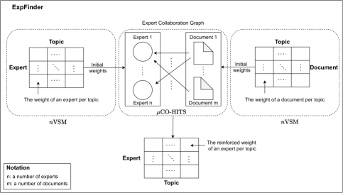
Figure 1: The overview of ExpFinder

Identifying experts given a query topic, known as expert finding, is a crucial task that accelerates rapid team formation for research innovations or business growth. Existing expert finding models can be classified into three categories such as vector space models (VSM) [2, 3], document language models (DLM) [4, 5, 6], or graph-based models (GM) [7, 8, 9]. ExpFinder [1] is an ensemble model for expert finding which integrates a novel $N$-gram VSM ($n$VSM) with a GM ($\mu$CO-HITS)-a variant of the generalised CO-HITS algorithm [7].

As seen in Figure 1, ExpFinder has $n$VSM, a vector space model, as a key component that estimates the weight of an expert and a document given a topic by leveraging the Inverse Document Frequency (IDF) weighting [10] for $N$-gram words (simply $N$-grams). Another key component in ExpFinder is $\mu$CO-HITS that is used to reinforce the weights of experts and documents given a topic in $n$VSM using an Expert Collaboration Graph (ECG) that is a certain form of an expert social network. The output of ExpFinder is the reinforced weights of experts given topics.

ExpFinder is designed and developed to improve the performance for expert finding. In this paper, we highlight two main contributions to the expert finding community. First, we provide a comprehensive implementation detail of all steps taken in ExpFinder. It could also be used as an implementation guideline for developing various DLM-, VSM- and GM-based expert finding approaches. Second, we illustrate how ExpFinder works with a simple example, thus researchers and practitioners can easily understand ExpFinder’s design and implementation.

This paper is organised as follows. Section 2 describes ExpFinder’s architecture and functionalities. Section 3 demonstrates the procedural steps in ExpFinder. Section 4 provides the impact and conclusion of ExpFinder.

2 Functionality

ExpFinder is implemented in Python (version $\geq$ 3.6) with open-source libraries such as pandas, NumPy, scikit-learn, SciPy, nltk, and networkx. In this section, we present its architecture, key components, and their functionalities. The architecture of ExpFinder is presented in Figure 2 that consists of four key steps with the corresponding functions and their functional dependencies:

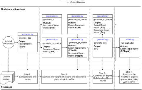
Figure 2: The architecture and functional workflow of ExpFinder: blue labels indicate module names of ExpFinder, and ‘Output Relation’ maps the functional component to the corresponding processing step.

1. Step 1 - Extract tokens and topics: Given an expertise source $\mathcal{D}$ (e.g., scientific publications) of experts $\mathcal{X}$, we extract expertise topics by using tokenise_doc() in extractor.py. We assume that expertise topics are represented in the forms of noun phrases. For each document $d\in\mathcal{D}$, the function splits it into sentences. Then, for each sentence, the function removes stopwords, assigns a part of speech (POS) to each word, merges the inflected forms of a word (i.e., the lemmatisation process, for example, ‘patients’ is lemmatised to ‘patient’), and extracts single-word terms (called tokens) and topics with a given linguistic pattern. In addition, we use a regular expression (regex) in Python to construct a linguistic pattern based on POS that is further used for extracting four different types of topics as shown in Figure 3.

   

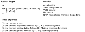
   Figure 3: The Python regular expression of a linguistic pattern for extracting topics in a single document

   Note that we use nltk for performing this process. The output of this step is the list of the tokens and the list of topics for each document $d\in\mathcal{D}$. The set of the all tokens is denoted as $\mathcal{W}$, and the set of the all topics is denoted as $\mathcal{T}$.

2. Step 2 - Estimate the weights of experts and documents given topics in $n$VSM: The process includes four main steps with the corresponding functions in generator.py:

   1. We use generate_tf() to estimate the term frequencies (TFs) of $\mathcal{W}$ in each document $d\in\mathcal{D}$. For this estimation, we use CountVectoerizer in scikit-learn. The output of this function is the $|\mathcal{D}|\times|\mathcal{W}|$ Document-Token matrix (DTM) where each entry contains the TF of $w\in\mathcal{W}$ in $d$.

   2. We use generate_dp_matrix() to estimate the weights of documents given $\mathcal{T}$ in $n$VSM [1]. The function estimates $n$TFIDF of each topic $t\in\mathcal{T}$ by integrating the $n$TF weighting and the $n$IDF weighting. Intuitively, $n$TF estimates the frequency of $t$ by averaging TFs of tokens in $t$ where TF of each token is stored in DTM. In addition, $n$IDF [10] is the $N$-gram IDF weighting method that estimates the log-IDF, $\log\frac{|\mathcal{D}|\times df(t)+1}{df(w_{1}\land w_{2}\land\ldots\land w_{n})^{2}+1}+1$, of $t$ where $w_{1},\ldots,w_{n}$ are $n$-constituent terms in $t$. The output of this step is the $|\mathcal{D}|\times|\mathcal{T}|$ Document-Phrase matrix (DPM) where each entry contains the $n$TFIDF weight of $t$ in $d$.

   3. Given $\mathcal{D}$, we use genenerate_ed_matrix() to generate the $|\mathcal{X}|\times|\mathcal{D}|$ Expert-Document matrix (EDM) where each entry shows a binary relationship between $x\in\mathcal{X}$ and $d$ (e.g., 1 indicates that $x$ has the authorship on $d$, and 0 otherwise).

   4. We use generate_pr_matrix() to estimate the weights of experts $\mathcal{X}$ and documents $\mathcal{D}$ given each topic $t\in\mathcal{T}$ in $n$VSM [1]. The weights of $\mathcal{X}$ are estimated by calculating matrix multiplication of $\textbf{EDM}^{|\mathcal{X}|\times|\mathcal{D}|}$ and $\textbf{DPM}^{|\mathcal{D}|\times|\mathcal{T}|}$ (e.g., ETopM = numpy.matmul(EDM, DPM) in Python). The output is the $|\mathcal{X}|\times|\mathcal{T}|$ Expert-Topic matrix (ETopM) where each entry contains the topic-sensitive weight of $x$ given $t$. The weights of $\mathcal{D}$ are represented by DPM. Now, we denote DPM as the $|\mathcal{D}|\times|\mathcal{T}|$ Document-Topic matrix (DTopM) where each entry shows the topic-sensitive weight of $d$ given $t$. It is worth noting that DPM can be integrated with another factor (e.g., the average document frequencies of $\mathcal{T}$) to obtain different weights for DTopM. However, in our approach, we set $\textbf{DTopM}=\textbf{DPM}$.

3. Step 3 - Construct ECG. We use generate_ecg() in generator.py to handle this step. The function receives $\mathcal{D}$ and builds an ECG using DiGraph in networkx to present a directed, weighted bipartite graph that has expert nodes $V_{x}$ and document nodes $V_{d}$. The set of nodes in the graph is denoted as $V$ such that $V=V_{x}\cup V_{d}$. A directed edge points from a document node $v_{d}\in V_{d}$ to an expert node $v_{x}\in V_{x}$ if $x$ has published $d$. In this step, we also use generate_ed_vector() in generator.py to generate a $|V|\times 1$ Expert-Count vector ($\boldsymbol{c_{x}}$) and a $|V|\times 1$ Document-Count ($\boldsymbol{c_{d}}$) vector based on ECG. These vectors are used for the estimation of $\mu$CO-HITS in Step 4.

4. Step 4 - Reinforce expert weights using $\mu$CO-HITS. We use run_expfinder() in trainer.py to handle this step. The function receives ETopM, DTopM, ECG, $\boldsymbol{c_{x}}$ and $\boldsymbol{c_{d}}$, generated in (Steps 2 and 3) as parameters, and reinforces the estimation of expert weights given topics by integrating $n$VSM and $\mu$CO-HITS [1]. For each $t\in\mathcal{T}$, we perform the three steps:

   1. Generate the adjacency matrix of nodes and its transpose - Given the ECG, we use to_matrix() in networkx to generate the $|V|\times|V|$ adjacency matrix of the graph M, and also construct its transpose matrix $\textbf{M}^{\top}$. These matrices are required in the initialisation for running the $\mu$CO-HITS algorithm.

   2. Normalise the weights of experts and documents given a topic - We get topic-sensitive weights of $\mathcal{X}$ and $\mathcal{D}$ given $t$ from ETopM and DTopM, respectively. The output of this includes the $|\mathcal{X}|\times 1$ Expert-Topic ($\boldsymbol{\alpha_{x}}$) and $|\mathcal{D}|\times 1$ Document-Topic ($\boldsymbol{\alpha_{d}}$) vectors where each entry shows the topic-sensitive weight of an expert and a document given $t$, respectively. Then, we normalise these vectors using L2 normalisation to scale their squares sum to 1 as the initialisation for running the $\mu$CO-HITS algorithm [11].

   3. Reinforce expert weights given a topic - We integrate $n$VSM and $\mu$CO-HITS through $k$ iterations to reinforce expert weights given $t$. $\mu$CO-HITS is the extension of the CO-HITS algorithm [7] which contains two main properties such as average authorities $\boldsymbol{a}$ and average hubs $\boldsymbol{h}$ which show importance of $\mathcal{X}$ and $\mathcal{D}$, respectively, based on the ECG. In addition, these properties can be defined as [1]:

      $$\boldsymbol{a}(\mathcal{X};t)^{k} =(1-\lambda_{x})\boldsymbol{a}(\mathcal{X};t)^{k-1}+\lambda_{x}\left(\frac{\textbf{M}^{\top}\boldsymbol{\cdot}\boldsymbol{h}(\mathcal{D};t)^{k-1}}{\boldsymbol{c_{d}}}\right)$$ (1)

      $$\boldsymbol{h}(\mathcal{D};t)^{k} =(1-\lambda_{d})\boldsymbol{h}(\mathcal{D};t)^{k-1}+\lambda_{d}\left(\frac{\textbf{M}\boldsymbol{\cdot}\boldsymbol{a}(\mathcal{X};t)^{k}}{\boldsymbol{c_{x}}}\right)$$ (2)

      where

      • $\boldsymbol{a}(\mathcal{X};t)^{k}$ and $\boldsymbol{h}(\mathcal{D};t)^{k}$ are $|V|\times 1$ vectors which contain the reinforced expert weights and reinforced document weights, respectively, given $t$ at $k^{\text{th}}$ iteration. As the initial weights of these vectors, we use the topic-sensitive weights of experts and documents estimated in $n$VSM. Thus, $\boldsymbol{a}(\mathcal{X};t)^{0}=\boldsymbol{\alpha_{x}}$ and $\boldsymbol{h}(\mathcal{D};t)^{0}=\boldsymbol{\alpha_{d}}$. By doing so, we integrate $n$VSM with $\mu$CO-HITS. Note that $\boldsymbol{a}(\mathcal{X};t)^{0}$ is a $|\mathcal{X}|\times 1$ vector, and $\boldsymbol{h}(\mathcal{D};t)^{0}$ is a $|\mathcal{D}|\times 1$ vector. However, for easily implementing the HITS algorithm, we have transformed the dimension of these vectors into $|V|\times 1$ vectors where additional entries hold the value of 0.

      • $\lambda_{x}\in[0,1]$ and $\lambda_{d}\in[0,1]$ are parameters for expert and document, respectively. These are used to control the impact of topic-sensitive weights on $\boldsymbol{a}$ and $\boldsymbol{h}$, respectively. Assigning lower values indicates the higher impact of topic-sensitive weights on $\boldsymbol{a}$ and $\boldsymbol{h}$.

      • $\left(\frac{\textbf{M}^{\top}\boldsymbol{\cdot}\boldsymbol{h}(\mathcal{D};t)^{k-1}}{\boldsymbol{c_{d}}}\right)$ is the calculation for the average authorities. The numerator performs matrix multiplication between the $|V|\times|V|$ adjacency matrix $\textbf{M}^{\top}$ and the $|V|\times 1$ $\boldsymbol{h}$. The denominator is a $|V|\times 1$ counted vector $\boldsymbol{c_{d}}$ generated in Step 3. To calculate this in Python, we simply apply numpy.matmul($\textbf{M}^{\top}$, $\boldsymbol{h}(\mathcal{D};t)^{k-1}$)/$\boldsymbol{c_{d}}$.

      • $\left(\frac{\textbf{M}\boldsymbol{\cdot}\boldsymbol{a}(\mathcal{X};t)^{k}}{\boldsymbol{c_{x}}}\right)$ is the calculation for the average hubs. The numerator performs matrix multiplication between the $|V|\times|V|$ adjacency matrix M and the $|V|\times 1$ $\boldsymbol{a}$. The denominator is a $|V|\times 1$ counted vector $\boldsymbol{c_{x}}$ generated in Step 3. To calculate this in Python, we simply apply numpy.matmul(M, $\boldsymbol{a}(\mathcal{X};t)^{k}$)/$\boldsymbol{c_{x}}$.

      After computing $\boldsymbol{a}$ and $\boldsymbol{h}$ at $k^{\text{th}}$ iteration, we apply L2 normalisation to both $\boldsymbol{a}$ and $\boldsymbol{h}$. We use the obtained $\boldsymbol{a}(\mathcal{X};t)$ after the final iteration to construct the $|\mathcal{X}|\times|\mathcal{T}|$ Expert-Topic matrix (RETopM) where each entry contains the reinforced weight of $x$ given $t$.

3 Illustrative examples

In this section, we illustrate how ExpFinder works. The input data includes three experts (i.e., $x_{1}$, $x_{2}$ and $x_{3}$) and three documents (i.e., $d_{1}$, $d_{2}$ and $d_{3}$) as shown in Table 1. Figure 4 presents the output examples of the steps in ExpFinder:

Docs	Experts	Text
$d_{1}$	$x_{1}$, $x_{2}$	A prerequisite for using electronic health records (EHR) data within learning health-care system is an infrastructure that enables access to EHR data longitudinally for health-care analytics and real time for knowledge delivery. Herein, we share our institutional implementation of a big data-empowered clinical natural language processing (NLP) infrastructure, which not only enables healthcare analytics but also has real-time NLP processing capability.
$d_{2}$	$x_{1}$, $x_{3}$	Word embedding, where semantic and syntactic features are captured from unlabeled text data, is a basic procedure in Natural Language Processing (NLP). In this paper, we first introduce the motivation and background of word embedding and its related language models.
$d_{3}$	$x_{2}$	Structural health monitoring at local and global levels using computer vision technologies has gained much attention in the structural health monitoring community in research and practice. Due to the computer vision technology application advantages such as non-contact, long distance, rapid, low cost and labor, and low interference to the daily operation of structures, it is promising to consider computer vision structural health monitoring as a complement to the conventional structural health monitoring. This article presents a general overview of the concepts, approaches, and real-life practice of computer vision structural health monitoring along with some relevant literature that is rapidly accumulating.

Table 1: The document dataset $\mathcal{D}$ used in the example: extracted phrases are highlighted in yellow, and extracted tokens are in bold.

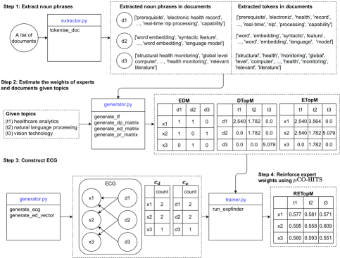
Figure 4: Illustrative examples for ExpFinder: the blue labels indicate module names of ExpFinder.

1. Step 1 - Extract tokens and topics: Given $\mathcal{D}$, we extract tokens $\mathcal{W}$ and topics $\mathcal{T}$. In this step, we set a maximum length of phrase to be 3 such that we only obtain phrases that have less than or equal to 3 tokens. Additionally, we use the linguistic pattern presented in Section 2. The output of this step contains the set of 50 unique topics $\mathcal{T}$ and the set of 85 unique tokens $\mathcal{W}$. For example, extracted topics in $d_{1}$ include some single-token topics (e.g., prerequisite and capability) and some multi-token topics (e.g., real-time nlp processing and electronic health record).

2. Step 2 - Estimate the weights of experts and documents given topics - Given $\mathcal{T}$ and $\mathcal{W}$, we generate three main matrices (i.e., EDM, DTopM and ETopM) that will also be used in Step 4. To do this, we perform the following:

   • Given $\mathcal{W}$, we generate $\textbf{DTM}^{3\times 85}$ where each entry shows the TF of a token $w\in\mathcal{W}$ in a document $d\in\mathcal{D}$. For example, the $3\times 1$ vector of healthcare, $\textbf{DTM}_{*,\texttt{healthcare}}$, is $(1,0,0)$ which shows it occurs only in $d_{1}$ (see also $\mathcal{D}$ in Table 1). As another example, we obtain $\textbf{DTM}_{*,\texttt{analytics}}=(2,0,0)$ which denotes that analytics appears twice in $d_{1}$.

   • Given $\mathcal{T}$ and $\textbf{DTM}^{3\times 85}$, we generate $\textbf{DPM}^{3\times 50}$ where each entry contains the weight of a phrase $t\in\mathcal{T}$ for a document calculated in $n$VSM. For example, suppose that health analytics is denoted as $t_{1}$, we then calculate $n$TF of $t_{1}$ in $d_{1}$ as:

     $$n\text{TF}(t_{1},d_{1})=\frac{\textbf{DTM}_{1,\texttt{healthcare}}+\textbf{DTM}_{1,\texttt{analytics}}}{|t_{1}|}\ =\frac{(1+2)}{2}=1.5$$

     where $|t_{1}|$ is a number of tokens in $t_{1}$. Then, we calculate the $N$-gram IDF of $t_{1}$ as:

     $$n\text{IDF}(t_{1}) =\log{\frac{|D|\cdot df(t_{1})+1}{df(\textbf{DTM}_{*,\texttt{healthcare}}\land\textbf{DTM}_{*,\texttt{analytics}})^{2}+1}}+1$$

     $$=\log{\frac{3\times 1+1}{df((1,0,0)\land(2,0,0))^{2}+1}}+1$$

     $$=\log{\frac{4}{1^{2}+1}}+1=1.693.$$

     Here, $\land$ is implemented in NumPy. Finally, we multiply $n\text{TF}(t_{1},d_{1})$ with $n\text{IDF}(t_{1})$ to obtain $n$TFIDF of $d_{1}$ given $t_{1}$ as: $\textbf{DPM}_{1,t_{1}}=n\text{TFIDF}(t_{1},d_{1})=n\text{TF}(t_{1},d_{1})\times n\text{IDF}(t_{1})=1.5\times 1.693=2.540$.

   • Given $\mathcal{D}$, we generate $\textbf{EDM}^{3\times 3}$ where each entry shows the authorship of an expert on a document. For example, $x_{1}$ is an author of $d_{1}$, and hence, the entry between $x_{1}$ and $d_{1}$ ($\textbf{EDM}_{1,1}$) equals 1. Also, $\textbf{EDM}_{1,3}=0$ shows that $x_{1}$ is not an author of $d_{3}$ (See Table 1).

   • Given $\textbf{EDM}^{3\times 3}$ and $\textbf{DPM}^{3\times 50}$, we generate $\textbf{ETopM}^{3\times 50}$ where each entry contains $n$TFIDF weight of an expert given a topic. As we explained in Section 2, we assume that $\textbf{DTopM}=\textbf{DPM}$. Now, we demonstrate the calculation for the weights of experts $\mathcal{X}$ given $t_{1}$ ($\textbf{ETopM}_{*,t_{1}}$) in $n$VSM as:

     $$\textbf{ETopM}_{*,t_{1}} =\textbf{EDM}^{3\times 3}\boldsymbol{\cdot}\textbf{DTopM}_{*,t_{1}}$$

     $$=\begin{bmatrix}1&1&0\\ 1&0&1\\ 0&1&0\end{bmatrix}\boldsymbol{\cdot}(2.540,0,0)=(2.540,2.540,0)$$

   Note that $\textbf{DTopM}^{3\times 3}$ and $\textbf{ETopM}^{3\times 3}$ are only used for the visualisation purpose. We use $\textbf{DTopM}^{3\times 50}$ and $\textbf{ETopM}^{3\times 50}$ for the estimation in Step 4.

3. Step 3 - Construct ECG: Given $\mathcal{D}$, we generate an ECG which has three expert nodes and three document nodes, as shown in Figure 4. The graph is also used to generate $3\times 1$ vectors (i.e., $\boldsymbol{c_{x}}$ and $\boldsymbol{c_{d}}$) that are used for the estimation of $\mu$CO-HITS in Step 4. For example, $\boldsymbol{c_{d}}_{1}=2$ indicates there are two documents (i.e., $d_{1}$ and $d_{2}$) pointing to $x_{1}$. Similarly, $\boldsymbol{c_{x}}_{3}=1$ indicates that there is one expert (i.e., $x_{2}$) who has authorship on $d_{3}$.

4. Step 4 - Reinforce expert weights using $\mu$CO-HITS: We use run_expfinder() in trainer.py to reinforce expert weights given topics $\mathcal{T}$. The function receives $\textbf{DTopM}^{3\times 50}$, $\textbf{ETopM}^{3\times 50}$, ECG, $\boldsymbol{c_{x}}$ and $\boldsymbol{c_{d}}$, generated in (Steps 2 and 3) as parameters, and generate the $3\times 50$ Expert-Topic matrix where each entry shows the reinforced weight of an expert given a topic. Now, we illustrate the estimation for the reinforced weight of $\mathcal{X}$ given $t_{1}$ as:

   • Given 6 nodes in an ECG, we generate the adjacency matrix $\textbf{M}^{6\times 6}$ and its transpose matrix $\textbf{M}^{\top}$ as:

     $$\textbf{M}=\begin{bmatrix}0&1&1&0&0&0\\ 0&0&0&0&0&0\\ 0&0&0&0&0&0\\ 0&1&0&0&1&0\\ 0&0&0&0&0&0\\ 0&0&1&0&0&0\end{bmatrix},\textbf{M}^{\top}=\begin{bmatrix}0&0&0&0&0&0\\ 1&0&0&1&0&0\\ 1&0&0&0&0&1\\ 0&0&0&0&0&0\\ 0&0&0&1&0&0\\ 0&0&0&0&0&0\end{bmatrix}$$

     where rows and columns are labeled with the sequence $\boldsymbol{s}$ (i.e., $\boldsymbol{s}=(d_{1},x_{1},x_{2},d_{2},x_{3},d_{3})$).

   • We apply L2 normalisation for the $6\times 1$ Expert-Topic ($\boldsymbol{\alpha_{x}}$) and the $6\times 1$ Document-Topic ($\boldsymbol{\alpha_{d}}$) vectors. The output of each vector is as:

     $$\boldsymbol{\alpha_{x}} =\texttt{L2-normalize}(\textbf{ETopM}_{*,t_{1}})=(0,0.707,0.707,0,0,0)$$

     $$\boldsymbol{\alpha_{d}} =\texttt{L2-normalize}(\textbf{DTopM}_{*,t_{1}})=(1,0,0,0,0,0)$$

   • We reinforce expert weights given $t_{1}$ in 5 iterations with $\lambda_{x}=1$ and $\lambda_{d}=0.7$. Here, we demonstrate the calculation of average authorities $\boldsymbol{a}$ and average hubs $\boldsymbol{h}$ at the first iteration ($k=1$):

     $$\boldsymbol{a}(\mathcal{X};t_{1})^{1} =(1-\lambda_{x})\boldsymbol{a}(\mathcal{X};t_{1})^{0}+\lambda_{x}\left(\frac{\textbf{M}^{\top}\boldsymbol{\cdot}\boldsymbol{h}(\mathcal{D};t_{1})^{0}}{\boldsymbol{c_{d}}}\right)$$

     $$=0\cdot(0,0.707,0.707,0,0,0)+1.0\cdot\left(\frac{(0,2,2,0,1,0)}{(2,1,1,2,1,1)}\right)$$

     $$=(0,2,2,0,1,0)$$

     $$\boldsymbol{h}(\mathcal{D};t_{1})^{1} =(1-\lambda_{d})\boldsymbol{h}(\mathcal{D};t_{1})^{0}+\lambda_{d}\left(\frac{\textbf{M}\boldsymbol{\cdot}\boldsymbol{a}(\mathcal{X};t_{1})^{1}}{\boldsymbol{c_{x}}}\right)$$

     $$=0.3\cdot(1,0,0,0,0,0)+0.7\cdot\left(\frac{(4,0,0,3,0,2)}{(1,2,2,1,1,1)}\right)$$

     $$=(3.1,0,0,2.1,0,1.4)$$

     where $\boldsymbol{a}(\mathcal{X};t_{1})^{1}$ and $\boldsymbol{h}(\mathcal{D};t_{1})^{1}$ are $6\times 1$ vectors. At the end of the iteration, we normalise these vectors by applying the L2 normalisation technique as:

     $$\boldsymbol{a}(\mathcal{X};t_{1})^{1} =\texttt{L2-normalize}(\boldsymbol{a}(\mathcal{X};t_{1})^{1})=(0,0.667,0.667,0,0.333,0)$$

     $$\boldsymbol{h}(\mathcal{D};t_{1})^{1} =\texttt{L2-normalize}(\boldsymbol{h}(\mathcal{D};t_{1})^{1})=(0.776,0,0,0.525,0,0.35)$$

     After 5 iterations, we obtain $\boldsymbol{a}(\mathcal{X};t_{1})^{5}=(0,0.577,0.595,0,0.56,0)$ whose labels are presented by $\boldsymbol{s}$, and hence, we use $x_{1}$, $x_{2}$ and $x_{3}$ as indexes for obtaining a $3\times 1$ vector (i.e., $\textbf{RETopM}_{*,t_{1}}=(0.577,0.595,0.56)$).

   The output is $\textbf{RETopM}^{3\times 50}$. If we use $t_{1}$ and the other two topics (i.e., natural language processing and vision technology, denoted as $t_{2}$ and $t_{3}$, respectively), we can generate $\textbf{RETopM}^{3\times 3}$ in Figure 4. This matrix can be used for two major tasks (1) finding the most expertise query for each expert (also known as expert profiling); and (2) finding the best expert for a given query (also known as expert finding).

4 Impact and Conclusion

With the growth of expertise digital sources, expert finding is a crucial task that has significantly helped people to seek the services and guidance of an expert [12]. ExpFinder is an ensemble model for expert finding that integrates $n$VSM with $\mu$CO-HITS to enhance the capability for expert finding over existing DLM, VSM and GM approaches. To our best knowledge, ExpFinder is the first attempt to provide the implementation of $n$VSM and $\mu$CO-HITS for expert finding.

The implementation of ExpFinder also provides functionalities that can be potentially useful for implementing other expert finding models. For example, our tokenisation module for extracting noun phrases using a linguistic pattern based on a part of speech (POS) can be easily customised based on researchers’ purposes. The modules for building the presented Expert-Document matrix (EDM), Expert-Topic matrix (ETopM), and Document-Topic matrix (DTopM) can be usefully leveraged to represent relationships between experts and documents, experts and topics, and documents and topics. These relationships can be used to represent a collective information among experts, documents and topics and used to implement other graph-based expert finding models such as an author-document-topic (ADT) graph [8] and an expert-expert graph via topics.

We highlight that ExpFinder is a state-of-the-art model, substantially outperforming the following widely known and latest models for expert finding: document language models [4], probabilistic-based expert finding model [6]), graph-based models [7, 8, 9]. Thus, the ones who want to extend ExpFinder can harness our implementation for further improvement of ExpFinder.

We presented the architecture and implementation detail of ExpFinder with an illustrative example. This would help researchers and practitioners to better understand how ExpFinder is designed and implemented with its core functionalities.

5 Declaration of Competing Interest

The authors declare that they have no known competing financial interests or personal relationships that could have appeared to influence the work reported in this paper.

6 Current code version

Ancillary data table required for subversion of the codebase. Kindly replace examples in right column with the correct information about your current code, and leave the left column as it is.

Nr.	Code metadata description
C1	Current code version	v1.0
C2	Permanent link to code/repository used for this code version	https://github.com/Yongbinkang/ExpFinder
C3	Permanent link to Reproducible Capsule	https://doi.org/10.24433/CO.0133456.v1
C4	Legal Code License	MIT License (MIT)
C5	Code versioning system used	git
C6	Software code languages, tools, and services used	Python
C7	Compilation requirements, operating environments & dependencies	Python environment version 3.6 or above, pandas, networkx, NumPy, scikit-learn, nltk, SciPy, Torch, Transformers, SciBERT
C8	Link to developer documentation/manual	https://github.com/Yongbinkang/ExpFinder/blob/main/README.md
C9	Support email for questions	ykang@swin.edu.au, hungdu@swin.edu.au

Table 2: Code metadata

References

- [1] Y.-B. Kang, H. Du, A. R. M. Forkan, P. P. Jayaraman, A. Aryani, T. Sellis, Expfinder: An ensemble expert finding model integrating -gram vector space model and co-hits (2021). arXiv:2101.06821.
- [2] F. Riahi, Z. Zolaktaf, M. Shafiei, E. Milios, Finding expert users in community question answering, in: Proceedings of the 21st International Conference on World Wide Web, 2012, pp. 791–798.
- [3] C. T. Chuang, K. H. Yang, Y. L. Lin, J. H. Wang, Combining query terms extension and weight correlative for expert finding, in: 2014 IEEE/WIC/ACM International Joint Conferences on Web Intelligence (WI) and Intelligent Agent Technologies (IAT), Vol. 1, IEEE, 2014, pp. 323–326.
- [4] K. Balog, L. Azzopardi, M. de Rijke, A language modeling framework for expert finding, Information Processing & Management 45 (1) (2009) 1 – 19.
- [5] B. Wang, X. Chen, H. Mamitsuka, S. Zhu, Bmexpert Mining medline for finding experts in biomedical domains based on language model, IEEE/ACM Trans. Comput. Biol. Bioinformatics 12 (6) (2015) 1286–1294.
- [6] P. Cifariello, P. Ferragina, M. Ponza, WISER: A semantic approach for expert finding in academia based on entity linking, Information Systems 82 (2019) 1 – 16.
- [7] H. Deng, M. R. Lyu, I. King, A Generalized CO-HITS Algorithm and Its Application to Bipartite Graphs, in: Proceedings of the 15th ACM SIGKDD International Conference on Knowledge Discovery and Data Mining, 2009, p. 239–248.
- [8] S. D. Gollapalli, P. Mitra, C. L. Giles, Ranking experts using author-document-topic graphs, in: Proceedings of the 13th ACM/IEEE-CS Joint Conference on Digital Libraries, JCDL ’13, 2013, pp. 87–96.
- [9] D. Schall, A Social Network-Based Recommender Systems, Springer, 2015.
- [10] M. Shirakawa, T. Hara, S. Nishio, IDF for Word N-Grams, ACM Trans. Inf. Syst. 36 (1).
- [11] J. M. Kleinberg, Authoritative sources in a hyperlinked environment, Journal of the ACM (JACM) 46 (5) (1999) 604–632.
- [12] R. Gonçalves, C. F. Dorneles, Automated expertise retrieval: A taxonomy-based survey and open issues, ACM Computing Surveys (CSUR) 52 (5) (2019) 1–30.