Stable maps and hyperbolic links

Abstract.

A stable map of a closed orientable $3$-manifold into the real plane is called a stable map of a link in the manifold if the link is contained in the set of definite fold points. We give a complete characterization of the hyperbolic links in the $3$-sphere that admit stable maps into the real plane with exactly one (connected component of a) fiber having two singular points.

2020 Mathematics Subject Classification: 57R45; 57K10, 57K32, 57R05

Keywords: stable map, branched shadow, hyperbolic link.

Introduction

Let $f:M\to\mathbb{R}^{2}$ be a stable map of a closed orientable $3$-manifold $M$ into the real plane $\mathbb{R}^{2}$. It is well-known that the singular points of $f$ are classified into three types: definite fold, indefinite fold and cusp. In [11] Levine showed that the cusp points can always be eliminated by a homotopical deformation. This implies that every $M$ admits a stable map into $\mathbb{R}^{2}$ without cusp points. In the following, we only consider stable maps without cusp points. The properties of the other types of singular points reflect the global topology of the source manifold $M$ as follows. In [1] Burlet-de Rham showed that if $M$ admits a stable map into $\mathbb{R}^{2}$ with only definite fold points, then $M$ is a connected sum $\#_{g}(S^{2}\times S^{1})$ for some non-negative integer $g$, where the empty connected sum $\#_{0}(S^{2}\times S^{1})$ implies $S^{3}$. In general, each connected component of a fiber of a stable map $f:M\to\mathbb{R}^{2}$ contains at most two singular points, and a connected component of a fiber of $f$ containing exactly two singular points, both of which are indefinite fold, is one of types $\mathrm{II}^{2}$ and $\mathrm{II}^{3}$ singular fibers shown in Figure 1. For any stable map of $M$ into $\mathbb{R}^{2}$, there exists at most finitely many singular fibers of these types.

Figure 1. Types $\mathrm{II}^{2}$ and $\mathrm{II}^{3}$ singular fibers.

In [15] Saeki generalized the result of [1] showing that if $M$ admits a stable map into $\mathbb{R}^{2}$ with no $\mathrm{II}^{2}$ or $\mathrm{II}^{3}$ singular fibers, then $M$ is a graph manifold, and vice versa. Recall that a $3$-manifold is a graph manifold if and only if its Gromov norm is zero. Later, Costantino-Thurston [3] and Gromov [7] gave, independently, a linear lower bound of the number of types $\mathrm{II}^{2}$ and $\mathrm{II}^{3}$ singular fibers of stable maps of $M$ into $\mathbb{R}^{2}$ in terms of Gromov norm.

In the present paper, we are interested in stable maps of links. Again, let $f:M\to\mathbb{R}^{2}$ be a stable map. We note that the set $S(f)$ of singular points of $f$ forms a link in $M$, each of whose components consists only of exactly one type of singular points. When a link $L$ in $M$ is contained in the set of definite fold points of $f$, we say that $f$ is a stable map of $(M,L)$. In [15] Saeki showed that if $(M,L)$ admits a stable map with no singular fibers of type $\mathrm{II}^{2}$ or $\mathrm{II}^{3}$, then $L$ is a graph link, that is, the exterior of $L$ is a graph manifold, and vice versa. This implies that any stable map of a hyperbolic link $L$ in $M$ has at least one singular fiber of type $\mathrm{II}^{2}$ or $\mathrm{II}^{3}$. Recently, Ishikawa-Koda [8] gave a complete characterization of the hyperbolic links in $S^{3}$ admitting stable maps into $\mathbb{R}^{2}$ with a single singular fiber type $\mathrm{II}^{2}$ and no one of type $\mathrm{II}^{3}$, see Theorem 1.3. For other work on the study of links through stable maps, see e.g. [14, 9].

The following is the main theorem of this paper.

Theorem 0.1.

Let $L$ be a hyperbolic link in $S^{3}$. Then there exists a stable map $f:(S^{3},L)\to\mathbb{R}^{2}$ with $\mathrm{II}^{2}(f)=\emptyset$ and $|\mathrm{II}^{3}(f)|=1$ if and only if the exterior of $L$ is diffeomorphic to a $3$-manifold obtained by Dehn filling the exterior of one of the four links $L^{\prime}_{1},L^{\prime}_{2},L^{\prime}_{3}$ and $L^{\prime}_{4}$ in $S^{3}$ along some of $($possibly none of$)$ boundary tori, where $L^{\prime}_{1},L^{\prime}_{2},L^{\prime}_{3},L^{\prime}_{4}$ are depicted in Figure 2.

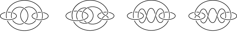
Figure 2. The links $L^{\prime}_{1},L^{\prime}_{2},L^{\prime}_{3}$ and $L^{\prime}_{4}$.

We note that the link $L^{\prime}_{1}$ above is the minimally twisted 5-chain link. All of the above links $L^{\prime}_{1},L^{\prime}_{2},L^{\prime}_{3},L^{\prime}_{4}$ are invariant by the rotation of $\pi$ around a horizontal axis. Theorem 0.1, together with the above result of Ishikawa-Koda [8], completes the characterization of the hyperbolic links in $S^{3}$ that admit stable maps into $\mathbb{R}^{2}$ with exactly one (connected component of a) fiber having two singular points. The proof is based on the connection between the Stein factorizations of stable maps and branched shadows developed in Costantino-Thurston [3] and Ishikwa-Koda [8]. Our proof is constructive, thus, as we will see in Corollary 3.1 we can actually describe the configuration of the fibers of the maps. We remark that the links $L^{\prime}_{1},L^{\prime}_{2},L^{\prime}_{3},L^{\prime}_{4}$ in Theorem 0.1 are all hyperbolic of volume $10v_{\mathrm{tet}}$, where $v_{\mathrm{tet}}=1.0149\cdots$ is the volume of the ideal regular tetrahedron. In fact, as was mentioned in Costantino-Thurston [3] we can find a decomposition of the complement of each of $L^{\prime}_{1},L^{\prime}_{2},L^{\prime}_{3},L^{\prime}_{4}$ into $10$ ideal regular tetrahedra. In the Appendix, we describe this decomposition explicitly.

1. Preliminaries

Throughout the paper, we will work in the smooth category unless otherwise mentioned. Let $Y$ be a subspace of a polyhedral space $X$. The symbolds $\operatorname{Nbd}(Y;X)$ and $\operatorname{Int}(Y)$ will denote a regular neighborhood of $Y$ in $X$ and the interior of $Y$ in $X$, respectively. The number of elements of a set $S$ is denoted by $|S|$.

1.1. Stable maps

Let $M$ be a closed orientable $3$-manifold. A smooth map $f$ of $M$ into $\mathbb{R}^{2}$ is said to be stable if there exists an open neighborhood of $f$ in $C^{\infty}(M,\mathbb{R}^{2})$ such that for any map $g$ in that neighborhood there exist diffeomorphisms $\Phi:M\to M$ and $\varphi:\mathbb{R}^{2}\to\mathbb{R}^{2}$ satisfying $g=\varphi\circ f\circ\Phi^{-1}$, where $C^{\infty}(M,\mathbb{R}^{2})$ is the set of smooth maps of $M$ into $\mathbb{R}^{2}$ with the Whitney $C^{\infty}$ topology. We denote by $S(f)$ the set of singular points of $f$, that is, $S(f)=\{p\in M\mid\mathrm{rank}~{}df_{p}<2\}$. The stable maps form an open dense set in the space $C^{\infty}(M,\mathbb{R}^{2})$, see Mather [13].

Proposition 1.1 (see e.g. Levine [12]).

Let $M$ be a closed-orientable $3$-manifold. Then a smooth map $f:M\to\mathbb{R}^{2}$ is stable if and only if $f$ satisfies the following conditions $(1)$–$(6)$:

Local conditions:

There exist local coordinates centered at $p$ and $f(p)$ such that $f$ is locally described in one of the following way:

1. $(u,x,y)\mapsto(u,x)$;

2. $(u,x,y)\mapsto(u,x^{2}+y^{2})$;

3. $(u,x,y)\mapsto(u,x^{2}-y^{2})$;

4. $(u,x,y)\mapsto(u,y^{2}+ux-x^{3})$.

$($In the cases of $(1)$, $(2)$, $(3)$, and $(4)$, $p$ is called a regular point, a definite fold point, an indefinite fold point, and a cusp point, respectively.$)$

Global conditions:

Additionally, $f$ satisfies

1. $f^{-1}(f(p))\cap S(f)=\{p\}$ for a cusp point $p$; and

2. the restriction of $f$ to $S(f)-\{\mbox{cusp points}\}$ is an immersion with only normal crossings.

In [11] Levine showed that the cusp points of each stable map can be eliminated by a homotopical deformation, which implies that every 3-manifold admits a stable map into $\mathbb{R}^{2}$ without cusp points. We note that the set $S(f)$ forms a link in $M$. For general definition and properties of stable maps, see e.g. Levine [12], Golubitsky-Guillemin [6], and Saeki [16]. In the following, we only consider stable maps without cusp points.

Let $M$ be a closed orientable 3-manifold, and $f:M\to\mathbb{R}^{2}$ a stable map. We say that two points $p_{1}$ and $p_{2}$ are equivalent if they are contained in the same component of the fibers of $f$. We denote by $Q_{f}$ the quotient space of $M$ with respect to the equivalence relation and by $q_{f}$ the quotient map. We define the map $\bar{f}:Q_{f}\to\mathbb{R}^{2}$ so that $f=\bar{f}\circ q_{f}$. The quotient space $Q_{f}$ is called the Stein factorization of $f$. By Kushner-Levine-Porto [10] and Levine [12] the local models of the Stein factorization $Q_{f}$ can be described as in Figure 3.

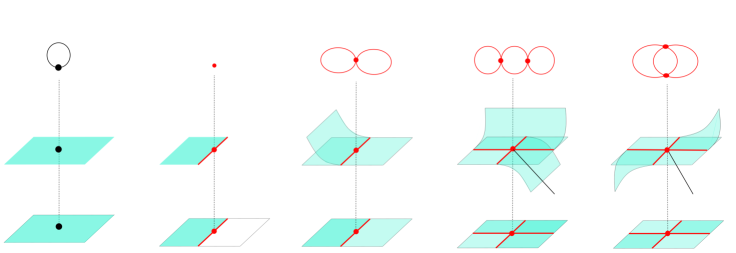
Figure 3. The Stein factorization of a stable map.

As shown in the figure, there are two types of (connected components of) singular fibers containing exactly two indefinite points. The one shown in Figure (iv) ((v), respectively) is called a singular fiber of type $\mathrm{II}^{2}$ ($\mathrm{II}^{3}$, respectively). We sometimes call a singular fiber of type $\mathrm{II}^{2}$ or $\mathrm{II}^{3}$ a codimension-$2$ singular fiber. We denote by $\mathrm{II}^{2}(f)$ and $\mathrm{II}^{3}(f)$ the sets of singular fibers of types $\mathrm{II}^{2}$ and $\mathrm{II}^{3}$ of $f$, respectively. We note that both $\mathrm{II}^{2}(f)$ and $\mathrm{II}^{3}(f)$ are finite sets. Further, we call a vertex of the Stein factorization $Q_{f}$ corresponding to a singular fiber of type $\mathrm{II}^{2}$ ($\mathrm{II}^{3}$, respectively) a vertex of type $\mathrm{II}^{2}$ ($\mathrm{II}^{3}$, respectively).

Definition.

Let $L$ be a link in a closed orientable $3$-manifold $M$. Then a stable map $f:M\to\mathbb{R}^{2}$ is called a stable map of $(M,L)$ if $L$ is contained in the set of definite fold points of $f$.

We note that for any link $L$ in a closed orientable $3$-manifold, there exists a stable map $f:(M,L)\to\mathbb{R}^{2}$, see e.g. Ishikawa-Koda [8].

In [15], Saeki gave a complete characterization of a link $L$ in a closed orientable $3$-manifold $M$ that admits a stable map $(M,L)\to\mathbb{R}^{2}$ without codimension-$2$ singular fibers as follows.

Theorem 1.2 (Saeki [15]).

Let $L$ be a link in a closed orientable $3$-manifold $M$. Then there exists a stable map $f:(M,L)\to\mathbb{R}^{2}$ with $\mathrm{II}^{2}(f)=\mathrm{II}^{3}(f)=\emptyset$ if and only if $L$ is a graph link.

By Theorem 1.2, any stable map of a hyperbolic link $L$ in a closed orientable 3-manifold has at least one singular fiber of type $\mathrm{II}^{2}$ or $\mathrm{II}^{3}$. The following theorem by Ishikawa-Koda [8, Theorem 5.6] gives a complete characterization of the hyperbolic links in $S^{3}$ admitting stable maps into $\mathbb{R}^{2}$ with a single singular fiber of type $\mathrm{II}^{2}$ and no one of type $\mathrm{II}^{3}$.

Theorem 1.3 (Ishikawa-Koda [8]).

Let $L$ be a hyperbolic link in $S^{3}$. Then there exists a stable map $f:(S^{3},L)\to\mathbb{R}^{2}$ with $|\mathrm{II}^{2}(f)|=1$ and $\mathrm{II}^{3}(f)=\emptyset$ if and only if the exterior of $L$ is diffeomorphic to a $3$-manifold obtained by Dehn filling the exterior of one of the six links $L_{1},L_{2},\ldots,L_{6}$ in $S^{3}$ along some of $($possibly none of$)$ boundary tori, where $L_{1},L_{2},\ldots,L_{6}$ are depicted in Figure 4.

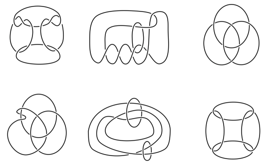
Figure 4. The links $L_{1},L_{2},\ldots,L_{6}$.

We note that the links $L_{1},L_{2},\ldots,L_{6}\subset S^{3}$ in Theorem 1.3 are all hyperbolic of volume $2v_{\mathrm{oct}}$, where $v_{\mathrm{oct}}=3.6638\cdots$ is the volume of the ideal regular octahedron. See the Appendix of this paper.

1.2. Branched shadows

A compact, connected polyhedron $P$ is called a simple polyhedron if every point of $P$ has a regular neighborhood homeomorphic to one of the four models shown in Figure 5.

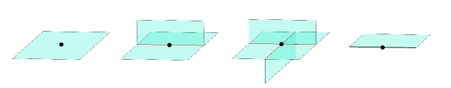
Figure 5. The local models of a simple polyhedron.

A point whose regular neighborhood is shaped on the model (iii) is called a vertex of $P$, and we denote the set of vertices of $P$ by $V(P)$. The set of points whose regular neighborhoods are shaped on the models (ii) or (iii) is called the singular set of $P$, and we denote it by $S(P)$. A component of $S(P)-V(P)$ is called an edge of $P$. We note that an edge is homeomorphic to either an open interval or a circle. The set of points whose regular neighborhoods are shaped on the model (iv) is called the boundary of $P$ and we denote it by $\partial P$. Each component of $X-S(P)$ is called a region of $P$. A region is said to be internal if it does not touch the boundary of $P$.

A branching of a simple polyhedron $P$ is the set of orientations on regions of $P$ such that the orientations on each edge of $P$ induced by the adjacent regions do not coincide. A branching of $P$ allows us to smoothen $P$ as shown in the local models in Figure 6.

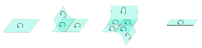
Figure 6. The local models of a branched polyhedron.

We call a simple polyhedron equipped with a branching a branched polyhedron.

Let $P$ be a simple polyhedron. A coloring of $\partial P$ is a map from the set of components of $\partial P$ to the set $\{i,e,f\}$ of three elements $i$ (internal), $e$ (external), and $f$ (false). Then with respect to the coloring, $\partial P$ decomposes into three peaces $\partial_{i}P$, $\partial_{e}P$, and $\partial_{f}P$. A simple polyhedron is said to be boundary-decorated if it is equipped with a coloring of $\partial P$.

Definition.

Let $M$ be a compact orientable $3$-manifold with $($possibly empty$)$ boundary consisting of tori. Let $L$ be a $($possibly empty$)$ link in $M$. A boundary-decorated simple polyhedron $P$ embedded in a compact oriented smooth $4$-manifold $W$ is called a shadow of $(M,L)$ if

1. $P$ is embedded in $W$ properly and smoothly, that is, $P\cap\partial W=\partial P$, and for each point $p$ in $P$, there exists a chart $(U,\varphi)$ of $W$ centered at $p$ such that $\varphi(U\cap P)\subset\{0\}\times\mathbb{R}_{+}^{3}\subset\mathbb{R}_{+}^{4}$ and $(\{0\}\times\mathbb{R}_{+}^{3},\varphi(U\cap P))$ is one of the four models in Figure 5 naturally regarded as being embedded in $\mathbb{R}_{+}^{3}$. Here we set $\mathbb{R}^{4}_{+}:=\{(x_{1},x_{2},x_{3},x_{4})\in\mathbb{R}^{4}\mid x_{4}\geq 0\}$ and $\{0\}\times\mathbb{R}^{3}_{+}:=(\{0\}\times\mathbb{R}^{3})\cap\mathbb{R}^{4}_{+}$.

2. $W$ collapses onto $P$ after equipping the natural PL structure on $W$;

3. $(M,L)=(\partial W-\operatorname{Int}\operatorname{Nbd}(\partial_{e}P;\partial W),\partial_{i}P)$.

In particular, when $P$ is a branched polyhedron, we call $P$ a branched shadow of $(M,L)$.

Under the above definition, we sometimes call $P$ a shadow of the $4$-manifold $W$. We note that a shadow of $E(L)$ is obtained from that of $(M,L)$ by just replacing the color $i$ (internal) with $e$ (external) of the boundary-decoration of $P$, but not vice versa. We denote by $\pi_{P}$ the map $M\to P$ obtained by restricting the collapsing map $W\searrow P$ in the above definition to $M$. We note that when $\partial M=\emptyset$, or equivalently, when $\partial_{e}(P)=\emptyset$, $\pi_{P}$ is a projection. We can assume that the map $\pi_{P}:M\to P$ satisfies the following:

• for each $p\in\partial_{i}P\cup\partial_{f}P$, $\pi_{P}^{-1}(p)$ is a single point;

• for each $p\in V(P)$, $\pi_{P}^{-1}(p)\cong T_{4}$, where $T_{4}$ is the suspension of four points;

• for each $p\in S(P)-V(P)$, $\pi_{P}^{-1}(p)\cong T_{3}$, where $T_{3}$ is the suspension of three points; and

• the restriction of $\pi_{P}$ to the preimage $\pi_{P}^{-1}(\pi_{P}(P)-S(P))$ is a smooth $S^{1}$-bundle over $\pi_{P}(P)-S(P)$.

By Turaev [17, 18], any pair $(M,L)$ of a compact orientable $3$-manifold $M$ with $($possibly empty$)$ boundary consisting of tori and a $($possibly empty$)$ link $L$ in $M$ has a shadow, see also Costantino [2]. As we will see in Example 1 below, when $L$ is a link in $S^{3}$, there is a standard way to obtain its branched shadow from a diagram of $L$.

Let $L$ be a $($possibly empty$)$ link in a compact orientable $3$-manifold $M$ with $($possibly empty$)$ boundary consisting of tori. Let $P\subset W$ be a shadow of $(M,L)$. To each internal region $R$ of $P$, we may assign a half-integer $\operatorname{gl}(R)$, called a gleam, as follows. Let $\iota:R\hookrightarrow W$ be the inclusion. Let $\bar{R}$ be the metric completion of $R$ with the path metric inherited from a Riemannian metric on $R$. For sinplicity, suppose that the natural extension $\bar{\iota}:\bar{R}\to M$ is injective. The germs $\operatorname{Nbd}(\bar{R};P)-P$ of the remaining regions near the circles $\partial\bar{R}$ give a structure of interval bundle over $\partial\bar{R}$, which is a sub-bundle of the normal bundle of $\partial\bar{R}$ in $W$. Let $\bar{R}^{\prime}$ be a generic small perturbation of $\bar{R}$ in $W$ such that $\partial\bar{R}^{\prime}$ lies in the interval bundle. The gleam $\operatorname{gl}(R)$ is then (well-)defined by counting the finitely many isolated intersections of $\bar{R}$ and $\bar{R}^{\prime}$ with signs as follows:

$$\operatorname{gl}(R)=\frac{1}{2}|\partial\bar{R}\cap\partial\bar{R}^{\prime}|+|\operatorname{Int}\bar{R}\cap\operatorname{Int}\bar{R}^{\prime}|\in\frac{1}{2}\mathbb{Z}.$$

We call a polyhedron $P$ equipped with a gleam on each internal region a shadowed polyhedron. In [17, 18], Turaev showed that the 4-manifold $W$, the 3-manifold $M\subset\partial W$ and the link $L\subset M$ are all recovered from a shadowed, boundary-decorated polyhedron $P$ in a canonical way.

Example 1.

Let $L=L_{1}\sqcup L_{2}\sqcup\cdots\sqcup L_{n}$ be an $n$-component link in $S^{3}$. Using a diagram of $L$, we can construct a shadow of $(S^{3},L)$ as in the following standard way.

We think of $S^{3}$ as the boundary of the $4$-ball $D^{4}=\{(z,w)\in\mathbb{C}^{2}\mid|z|^{2}+|w|^{2}\leq 1\}$. Set $D:=\{(z,w)\in D^{4}\mid w=0\}$, which is an oriented $2$-disk. Let $D^{\prime}$ be the closure of $D-\operatorname{Nbd}(\partial D;D)$. Let $\pi:S^{3}\to D$ be the projection induced by a collapsing $D^{4}\searrow D$. We can assume without loss of generality that the preimage $V=\pi^{-1}(D^{\prime})$ is a solid torus, which we identify with $D^{\prime}\times S^{1}$. We note that $S^{3}-\operatorname{Int}V$ is also a solid torus. We can push $L$ by isotopy so that $L$ lies in $D^{\prime}\times[[-\varepsilon],[\varepsilon]]$, where $S^{1}$ is identified with $\mathbb{R}/2\pi\mathbb{Z}$, $\varepsilon$ is a sufficiently small positive real number, and we assume that $\pi|_{V}$ is generic with respect to $L$. Thus, the image $\pi(L)$, together with over/under crossing information at each double point of $\pi(L)$, gives a diagram $D_{L}$ of $L$ on $D^{\prime}$. Consider the mapping cylinder

$$P_{D_{L}}^{*}=((L\times[0,1])\sqcup D^{\prime})/(x,0)\sim\pi(x).$$

Then $P_{D_{L}}^{*}$, together with the color $e$ (external) of each $L_{j}\times\{1\}\subset\partial P_{L}^{*}$ and the color $f$ (false) of the remaining boundary circle, is a shadow of $(S^{3},L)$. The set of the regions of $P_{D_{L}}^{*}$ consists of subsurfaces of $D^{\prime}$ and half-open annuli $A_{j}=L_{j}\times(0,1]$, $j\in\{1,2,\ldots,n\}$. The gleam on each internal region of $P_{D_{L}}^{*}$, which lies in $D^{\prime}$, is obtained by counting the local contributions around crossings as indicated in Figure 7. Refer to Turaev [18] and Costantino [2] for more details.

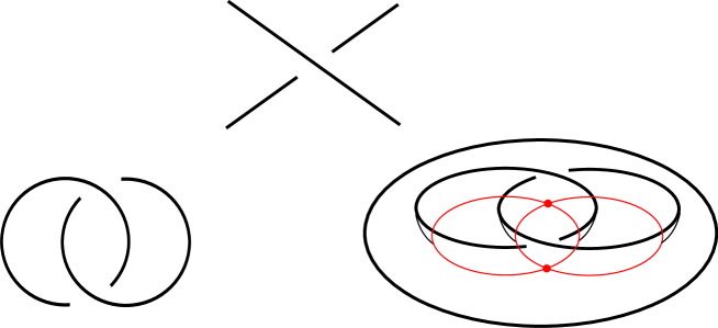
Figure 7. The diagram $D_{H}$ of the Hopf link $H$ and the branched shadow $P_{D_{H}}^{*}$.

To each region of $P_{D_{L}}^{*}$ contained in $D^{\prime}$, we give the orientation induced by the prefixed orientation of $D^{\prime}$. By equipping, further, orientations to the other regions $A_{1},A_{2},\ldots,A_{n}$ in an arbitrary way, $P_{D_{L}}^{*}$ becomes a branched shadow of $(S^{3},L)$. Let $R$ be the region of $P_{D_{L}}^{*}$ touching $\partial D^{\prime}$. Suppose that the branched polyhedron $P_{D_{L}}^{*}$ satisfies the following:

• the closure of $R$ is an annulus; and

• on each edge of $P_{D_{L}}^{*}$ touched by $R$ and $A_{j}$ ($j\in\{1,2,\ldots,n\}$), the orientations induced from those of $R$ and $A_{j}$ coincide.

We note that if we choose, for example, $D_{L}$ to be a closed braid presentation of $L$, we can find a branching of $P_{D_{L}}^{*}$ satisfying the above conditions. Then, $P_{D_{L}}:=P_{D_{L}}^{*}-R$ is still a branched polyhedron, thus, a branched shadow of $(S^{3},L)$. See Figure 8.

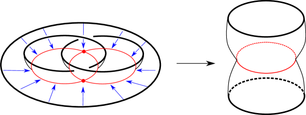
Figure 8. From $P_{D_{H}}^{*}$ to $P_{D_{H}}$.

Let $M$ be a compact orientable $3$-manifold $M$ with $($possibly empty$)$ boundary consisting of tori. Let $P\subset W$ be a shadow of $M=(M,\emptyset)$. Suppose for simplicity that all components of $\partial P$ is colored by $i$ (internal), and no component of $S(P)$ is a circle. Then the combinatorial structure of $P$ induces a decomposition of $P$ into pieces each of which is homeomorphic to one of

1. the model in Figure 5 (iii);

2. the model in Figure 5 (ii); or

3. a compact surface $F$.

Here, the pieces of (1) one-to-one correspond to the vertices of $P$, the pieces of (2) one-to-one correspond to the edges of $P$, and the pieces of (3) one-to-one correspond to the regions of $P$. We call this the combinatorial decomposition of $P$. The combinatorial decomposition then induces, through the preimage of the map $\pi_{P}:M\to P$, a decomposition of $M$ into pieces each of which is homeomorphic to one of

1. a handlebody of genus three;

2. a handlebody of genus two; or

3. an orientable $S^{1}$ bundle over a compact surface.

We note that each piece of $(2)$ here is naturally equipped with the product structure $R\times[0,1]$, where $R$ is a pair of pants, through $\pi_{P}^{-1}$.

2. Relationship between Stein factorizatons and branched shadows

From now until the end of the paper, $X$ always denotes the local part of a branched, shadowed polyhedron depicted in Figure 9, where $+1$ in the figure is the gleam on the bigon.

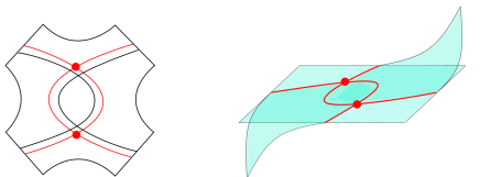
Figure 9. The local part $X$ of a branched, shadowed polyhedron.

Let $M$ be a closed orientable $3$-manifold. As we have seen in Section 1.1, each point of the Stein factorization of a stable map of $M$ into $\mathbb{R}^{2}$ is homeomorphic to one of the four local models shown in Figure 10.

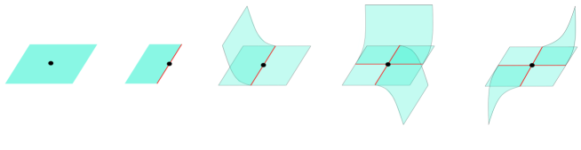
Figure 10. The local models of a Stein factorization.

From the figure, we see that the Stein factorization is “almost” a branched polyhedron. Indeed, the local models in Figure 10 coincide with those in Figure 6 except the model of Figure 10 (iv), which is a regular neighborhood of a vertex of type $\mathrm{II}^{3}$. Costantino-Thurston [3, Section 4] revealed that we can actually obtain a branched shadow from the Stein factorization of a stable map by replacing a regular neighborhood of each vertex of type $\mathrm{II}^{3}$ with $X$.

Theorem 2.1 (Costantino-Thurston [3]).

Let $L$ be a link in a closed orientable $3$-manifold $M$. Let $f:(M,L)\to\mathbb{R}^{2}$ be a stable map. Then a branched polyhedron $P$ obtained by replacing a regular neighborhood of each vertex of type $\mathrm{II}^{3}$ of $Q_{f}$ with $X$ as shown in Figure 11 is a branched shadow of $(M,L)$.

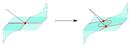
Figure 11. Replacement of a neighborhood of type $\mathrm{II}^{3}$ vertex with $X$.

In fact, in Theorem 2.1 the $4$-manifold $W$ containing $P$ as a shadow can be constructed from $f$ in a natural way, and $Q_{f}$ is already naturally embedded in $W$. The replacement in Theorem 2.1 can then be performed in $W$.

The following theorem by Ishikawa-Koda [8, Theorem 3.5, Lemma 3.12 and Corollary 3.13] is a sort of inverse of Theorem  2.1: we can construct a stable map from a branched shadow.

Theorem 2.2 (Ishikawa-Koda [8]).

Let $L$ be a link in a closed orientable $3$-manifold $M$. Let $P$ be a branched shadow of $E(L)$. Then there exists a stable map $f:(M,L)\to\mathbb{R}^{2}$ with $|\mathrm{II}^{2}(f)|=|V(P)|$ and $\mathrm{II}^{3}(f)=\emptyset$.

The proof of Theorem 2.2 given in [8] is constructive. We remark that the Stein factorization $Q_{f}$ of the stable map $f$ in Theorem 2.2 is possibly not homeomorphic to the given branched polyhedron $P$ in general. However, if we regard $Q_{f}$ as a branched polyhedron (this is possible because $\mathrm{II}^{3}(f)=\emptyset$), there exists a canonical embedding of $\operatorname{Nbd}(S(P);P)$ into $\operatorname{Nbd}(S(Q_{f});Q_{f})$. Further, if $P$ contains $X$, the Stein factorization $Q_{f}$ also contains $X$ at the corresponding part.

Example 2.

Let $P_{D_{H}}^{*}$ is a branched shadow of the Hopf link $H$ shown in Figure 7 in Example 1. Let $h:(S^{3},H)\to\mathbb{R}^{2}$ be a stable map constructed from $P_{D_{H}}^{*}$ by Theorem 2.2. Then we can identify the Stein factorization $Q_{h}$ with $P_{D_{H}}^{*}$. The fiber $q_{h}^{-1}(p)$ over each point $p\in P_{D_{H}}^{*}$ can be described as follows. Here, we recall that $q_{h}:S^{3}\to P_{D_{H}}^{*}$ is the quotient map. We use the same notation as in Example 1.

• If $p\in D^{\prime}-S(P_{D_{H}}^{*})$, then $q_{h}^{-1}(p)=\{p\}\times S^{1}\subset D^{\prime}\times S^{1}=V$. See Figure 12.

  

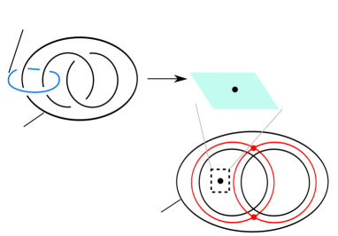
  Figure 12. The fiber of $q_{h}$ over $p\in D^{\prime}-S(P_{D_{H}}^{\ast})$.

• Let $K$ be a component of $H$. Let $p\in K\times\{1\}\subset P_{D_{H}}^{*}$ and $p_{1}\in K\times(0,1)\subset P_{D_{H}}^{*}$. Then $q_{h}^{-1}(p)$ is a point on $K$, while $q_{h}^{-1}(p_{1})$ is a meridian of $K$. See Figure 13.

  

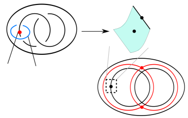
  Figure 13. The fibers of $q_{h}$ over $p\in K\times\{1\}$ and $p_{1}\in K\times(0,1)$.

• Let $p\in S(P_{D_{H}}^{*})-V(P_{D_{H}}^{*})$. Choose three points $p_{1},p_{2},p_{3}\in P_{D_{H}}^{*}$ near $p$ as in Figure 14. Then from the configuration of the fibers $q_{h}^{-1}(p_{1})$, $q_{h}^{-1}(p_{2})$, $q_{h}^{-1}(p_{3})$, we can find the configuration of $q_{h}^{-1}(p)$ as shown in Figure 14.

  

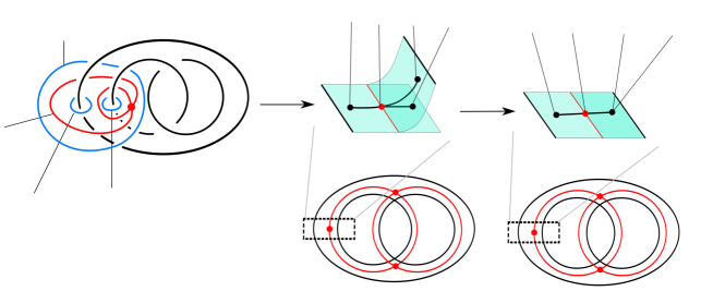
  Figure 14. The fiber of $q_{f}$ over $p\in S(P_{D_{H}}^{*})-V(P_{D_{H}}^{*})$.

• Let $p\in V(P_{D_{H}}^{*})$. Choose three points $p_{1},p_{2},p_{3},p_{4}\in P_{D_{H}}^{*}$ near $p$ as in Figure 15. Then from the configuration of the fibers $q_{h}^{-1}(p_{1})$, $q_{h}^{-1}(p_{2})$, $q_{h}^{-1}(p_{3})$, $q_{h}^{-1}(p_{4})$, we can find the configuration of $q_{h}^{-1}(p)$ as shown in Figure 15.

  

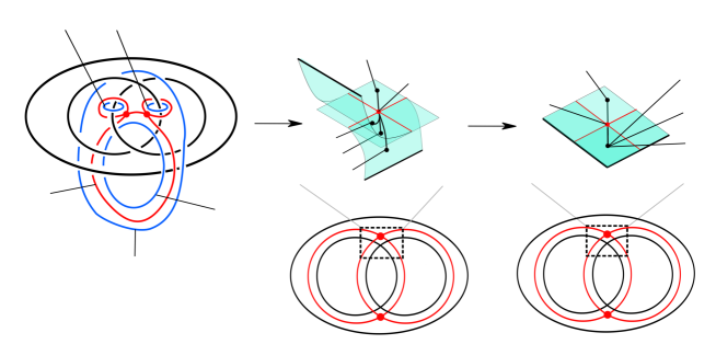
  Figure 15. The fiber of $q_{f}$ over $p\in V(P_{D_{H}}^{*})$.

Corollary 2.3.

Let $L$ be a link in a closed orientable $3$-manifold $M$. Let $P$ be a branched shadow of $E(L)$. Let $f:(M,L)\to\mathbb{R}^{2}$ be a stable map obtained from $P$ as in Theorem 2.2. Then there exists a stable map $g:(M,L)\to\mathbb{R}^{2}$ such that the Stein factorization $Q_{g}$ is obtained from $Q_{f}$ by replacing each part homeomorphic to $X$ with the model of Figure 10 (iv).

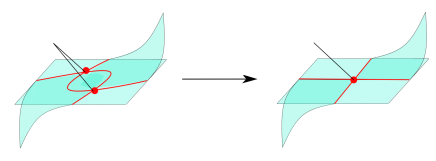
Figure 16. Replacement of $X$ with a neighborhood of type $\mathrm{II}^{3}$ vertex.

Proof.

Suppose that $Q_{f}$ contains a local part, which we simply denote by $X$, homeomorphic to $X$. As we have seen in Example 2, the fiber of $q_{f}$ over each point of the boundary of $X$ is as shown in Figure 17.

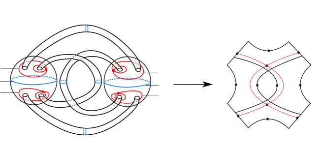
Figure 17. The fiber of $q_{f}$ over each point of the boundary of $X$.

Let $f^{\prime}:M\to\mathbb{R}^{2}$ be a stable map containing a singular fiber of type $\mathrm{II}^{3}$. Let $v$ be a type $\mathrm{II}^{3}$ vertex of the Stein factorization $Q_{f^{\prime}}$. Then the behavior of the map $f^{\prime}$ on the preimage of $\operatorname{Nbd}(v;Q_{f^{\prime}})$ under the quotient map $q_{f^{\prime}}$ is as drawn in Figure 18.

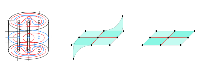
Figure 18. The Stein factorization of $f^{\prime}|_{q_{f^{\prime}}^{-1}(\operatorname{Nbd}(v;Q_{f^{\prime}}))}$.

We can assume that $\bar{f}(X)=\bar{f^{\prime}}(\operatorname{Nbd}(v;Q_{f^{\prime}}))$. We identify the boundary of $X$ and that of $\operatorname{Nbd}(v;Q_{f^{\prime}})$ naturally so that the map $\bar{f}$ coincides with $\bar{f^{\prime}}$ on the boundaries modulo the identification. We note that both $q_{f}^{-1}(X)$ and $q_{f^{\prime}}^{-1}(\operatorname{Nbd}(v;Q_{f^{\prime}}))$ are handlebodies of genus three. We define a diffeomorphism from $q_{f}^{-1}(X)$ to $q_{f^{\prime}}^{-1}(\operatorname{Nbd}(v;Q_{f^{\prime}}))$ using the handle slide shown on the bottom in Figure 19. We then identify the two handlebodies by this diffeomorphism and denote both of them by $V$. Under this identification, the fiber of $q_{f}$ over each point of the boundary of $X$ is identified with that of $q_{f^{\prime}}$ over a point of the boundary of $\operatorname{Nbd}(v;Q_{f^{\prime}})$ as indicated by the labels in Figure 19.

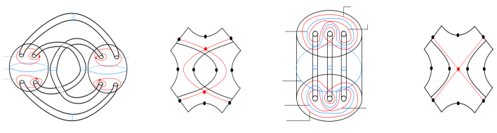
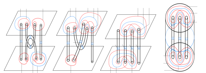
Figure 19. The fibers of $q_{f}$ over the points of the boundary of $X$ (top left) agree with those of $q_{f^{\prime}}$ over the points of the boundary of $\operatorname{Nbd}(v;Q_{f^{\prime}})$ (top right) after a handle slide (bottom).

This implies that $q_{f}|_{\partial V}$ coincides with $q_{f^{\prime}}|_{\partial V}$. Consequently, $f$ coincides with $f^{\prime}$ on the boundary of $V$. Thus, by gluing the maps $f|_{M-\operatorname{Int}V}$ and $f^{\prime}|_{V}$ and then smoothening it appropriately, we obtain a stable map $g:(M,L)\to\mathbb{R}^{2}$ satisfying $|\mathrm{II}^{2}(g)|=|\mathrm{II}^{2}(f)|-2$ and $|\mathrm{II}^{3}(g)|=1$. Applying the same argument for the other local parts of $Q_{f}$ homeomorphic to $X$ repeatedly, we finally get a desired stable map of $(M,L)$ into $\mathbb{R}^{2}$. ∎

3. The main theorem

We first show the ”only if” part of Theorem 0.1. Suppose that there exists a stable map $f:(S^{3},L)\to\mathbb{R}^{2}$ with $\mathrm{II}^{2}=\emptyset$ and $|\mathrm{II}^{3}|=1$. Let $P$ be a branched polyhedron obtained by replacing a regular neighborhood of each vertex of type $\mathrm{II}^{3}$ of $Q_{f}$ with $X$. By Theorem 2.1, $P$ is a branched shadow of $(S^{3},L)$. We note that, by this construction, the two vertices of $P$ is contained in a single component of the singular set $S(P)$. Let $c$ be the component of $S(P)$ containing the vertices of $P$. Set $P^{\prime}=\operatorname{Nbd}(c;P)\cup X$, which is also a branched polyhedron, where every region is a half-open annulus. By Ishikawa-Koda [8, Lemma 5.5], there exists a branched shadow $P^{\prime\prime}$ of $(S^{3},L)$ that is obtained from $P^{\prime}$ by attaching towers to some of its boundary components. Here, a tower is a simple polyhedron obtained by gluing several $2$-disks to an annulus as depicted in Figure 20.

Figure 20. A tower.

The branching of $P^{\prime}$ naturally extends to that of $P^{\prime\prime}$.

Claim 1.

$P^{\prime}$ is homeomporphic to one of the five branched polyhedra $P_{1},P_{2},\ldots,P_{5}$ depicted in Figure 21.

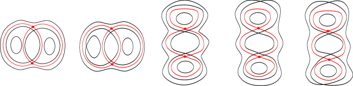
Figure 21. The branched polyhedra $P_{1},P_{2},\ldots,P_{5}$.

Proof of Claim 1.

Since $c$ is a $4$-valent graph with exactly $2$ vertices, $c$ is homeomorphic to one of the graphs of types $1$, $2$ and $3$ shown in Figure 22.

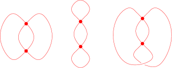
Figure 22. The $4$-valent graphs of types $1$, $2$ and $3$.

Suppose that $c$ is of type $3$. Using the combinatorial structure of $c$, $P^{\prime}$ is then obtained from $X$ by gluing subspaces of the boundary of $X$ according to the combinatorial structure around the edges of $P^{\prime}$, see Figure 23 for example.

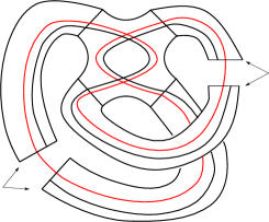
Figure 23. From $X$ to $P^{\prime}$.

However, as indicated in Figure 24, the branching of $X$ cannot be extended to that of $P^{\prime}$ no matter how we glue subspaces of the boundary of $X$ in the above process. This contradicts the fact that the branched polyhedron $P^{\prime}$ contains $X$.

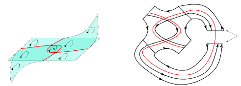
Figure 24. If $c$ is of type $3$, the branching of $X$ cannot be extended to that of $P^{\prime}$.

Therefore, $c$ must be of type $1$ or $2$. Then using the branching of $X$, we can check that $P^{\prime}$ is one of the polyhedra depicted in Figures 25 and 26.

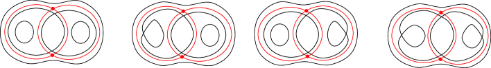
Figure 25. The candidates of $P^{\prime}$ when $c$ is of type $1$.

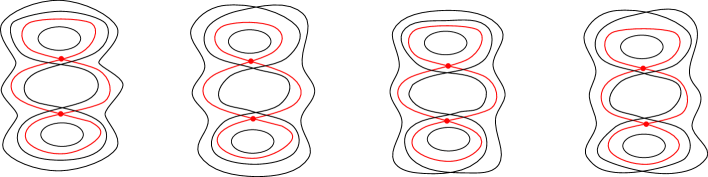
Figure 26. The candidates of $P^{\prime}$ when $c$ is of type $2$.

We note that after replacing the color $i$ (internal) with $f$ (false) of the boundary-decoration of $P^{\prime\prime}$, $P^{\prime\prime}$ becomes a shadow of $S^{3}$. Thus, $P^{\prime\prime}$ is simply connected by Ishikawa-Koda [8, Lemma 5.1]. Therefore, $P^{\prime}$ must be able to be simply connected by attaching towers to some of its boundary components. However, the branched polyhedron 1-(iv) in Figure 25 cannot be simply connected even though we attach a tower to every boundary component. Hence, we can remove 1-(iv) from the possible list of shapes of $P^{\prime}$. Further, the branched polyhedra 1-(ii) and 2-(ii) are homeomorphic to 1-(iii) and 2-(iii), respectively. Consequently, $P^{\prime}$ is homeomorphic to one of 1-(i), 1-(ii), 2-(i), 2-(ii) and 2-(iv). These are exactly the branched polyhedra $P_{1},P_{2},\ldots,P_{5}$ depicted in Figure 21. ∎

Claim 2.

The branched polyhedra $P_{1},P_{2},\ldots,P_{5}$ depicted in Figure 21 are, respectively, branched shadows of the exterior of the links $L_{1}^{\prime}$, $L_{2}^{\prime},\ldots,L_{5}^{\prime}$, where $L_{1}^{\prime},L_{2}^{\prime},L_{3}^{\prime},L_{4}^{\prime}$ are the links depicted in Figure 2, and $L^{\prime}_{5}$ is the one depicted in Figure 27.

Figure 27. The link $L^{\prime}_{5}$.

Proof of Claim 2.

Let $U_{1},U_{2},\ldots,U_{5}$ be diagrams of the trivial knot or the Hopf link illustrated in Figure 28.

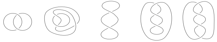
Figure 28. The diagrams $U_{1},U_{2},\ldots,U_{5}$ of the trivial knot or the Hopf link.

Let $P_{U_{1}}^{*}$, $P_{U_{2}}$, $P_{U_{3}}^{*}$, $P_{U_{4}}$, $P_{U_{5}}$ be the branched polyhedra obtained from $U_{1},U_{2},\ldots,U_{5}$ as in Example 1.

We first show that $P_{1}$ is a branched shadow of $E(L^{\prime}_{1})$. Define a coloring of $\partial P^{*}_{U_{1}}$ by $\partial_{e}P^{*}_{U_{1}}=\partial P^{*}_{U_{1}}$. The boundary $\partial P^{\ast}_{U_{1}}$ of $P^{\ast}_{U_{1}}$ forms a link in $S^{3}$, and $P^{\ast}_{U_{1}}$ is a branched shadow of the exterior $E(\partial P^{\ast}_{U_{1}})$ of the link $\partial P^{\ast}_{U_{1}}\subset S^{3}$. The branched polyhedron $P_{1}$ is obtained by removing the interior of the $2$-disks $D_{1}$ and $D_{2}$ shown in Figure 29. Recall the map $\pi_{P^{*}_{U_{1}}}$ defined in Section 1.2. The preimages of the disks $D_{1}$ and $D_{2}$ under $\pi_{P^{*}_{U_{1}}}$ are then solid tori shown in Figure 29.

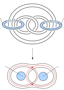
Figure 29. The $2$-disks $D_{1},D_{2}$ and their preimages under $\pi_{P^{*}_{U_{1}}}$.

As indicated in Figure 29, the space obtained from $E(\partial P^{\ast}_{U_{1}})$ by removing the interiors of the solid tori $\pi^{-1}(D_{1})$ and $\pi^{-1}(D_{2})$ is homeomorphic to $E(\partial P^{*}_{U_{1}})$. This implies that $P_{1}$ is a branched shadow of $E(L^{\prime}_{1})$.

The proof for the other cases runs in the same way. Indeed, the polyhedra $P_{2}$, $P_{3}$, $P_{4}$, $P_{5}$ can be obtained by removing the interiors of the $2$-disks from $P_{U_{2}}$, $P^{*}_{U_{3}}$, $P_{U_{4}}$, $P_{U_{5}}$ shown in Figure 30. Since the the preimages of those disks are as drawn in the same figure, we see that $P_{2}$, $P_{3}$, $P_{4}$, $P_{5}$ are branched shadows of $E(L^{\prime}_{2})$, $E(L^{\prime}_{3})$, $E(L^{\prime}_{4})$, $E(L^{\prime}_{5})$, respectively.

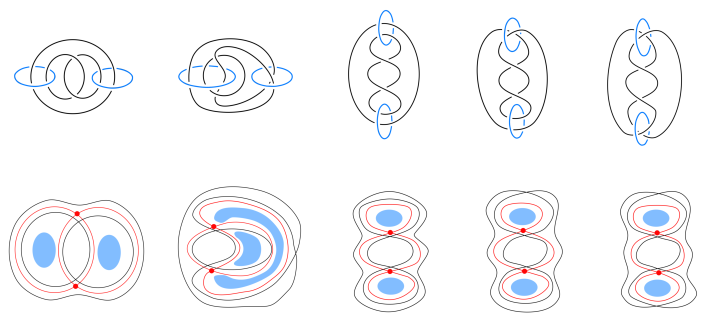
Figure 30. The preimages of $2$-disks.

∎

By Claim 1, $P^{\prime\prime}$ is homeomorphic to one of $P_{1},P_{2},\ldots,P_{5}$ depicted in Figure 21, or the one obtained by attaching towers to some of their boundary components. Thus, by Claim 2, together with Costantino-Thurston [3, Proposition 3.27], $E(L)$ is diffeomorphic to a $3$-manifold obtained by Dehn filling $E(L_{1}^{\prime}),E(L_{2}^{\prime}),\ldots,E(L_{5}^{\prime})$ along some of $($possibly none of$)$ boundary tori. Since SnapPy [4] tells us that the complements of the links $L^{\prime}_{3}$ and $L^{\prime}_{5}$ are homeomorphic, we can exclude $E(L_{5}^{\prime})$ from them.

Next, we show the “if” part of Theorem 0.1. Suppose that $E(L)$ is diffeomorphic to a $3$-manifold obtained by Dehn filling $E(L_{1}^{\prime}),E(L_{2}^{\prime}),E(L_{3}^{\prime}),E(L_{4}^{\prime})$ along some of $($possibly none of$)$ boundary tori. Let $P_{i}$ ($i=1,2,3,4$) be the branched shadow of $E(L^{\prime}_{i})$ shown in Figure 21. Then again by Costantino-Thurston [3, Proposition 3.27], we can obtain a branched shadow $P$ of $E(L)$ by attaching towers to some of (possibly, none of) the boundary components of $P_{i}$. By Theorem 2.2 to $P$, we can construct a stable map $f:(S^{3},L)\to\mathbb{R}^{2}$ from $P$. Then by Corollary 2.3, there exists a stable map $g:(S^{3},L)\to\mathbb{R}^{2}$ such that the Stein factorization $Q_{g}$ is obtained from $Q_{f}$ by replacing each part homeomorphic to $X$ with the model of Figure 10 (iv). Clearly, we have $\mathrm{II}^{2}(g)=\emptyset$ and $|\mathrm{II}^{3}(g)|=1$. This completes the proof of Theorem 0.1.

As we have seen in the above proof, for each link $L_{i}^{\prime}$ ($i=1,2,3,4$), we can construct a stable map $f_{i}:(S^{3},L_{i}^{\prime})\to\mathbb{R}^{2}$ with $\mathrm{II}^{2}(f_{i})=\emptyset$ and $|\mathrm{II}^{3}(f_{i})|=1$ explicitly. In particular, in this case, as we have seen in Example 2, $Q_{f_{i}}$ is obtained from $P_{i}$ by replacing the unique local part homeomorphic to $X$ with the model of Figure 10 (iv), and further, we can draw the configuration of fibers of $f_{i}$ explicitly. Consequently, we have the following.

Corollary 3.1.

For each link $L_{i}^{\prime}$ $($$i=1,2,3,4$$)$ shown in Figure 2, there exists a stable map $f_{i}:(S^{3},L^{\prime}_{i})\to\mathbb{R}^{2}$ with $\mathrm{II}^{2}(f_{i})=\emptyset$ and $|\mathrm{II}^{3}(f_{i})|=1$ such that the configuration of the unique singular fiber of type $\mathrm{II}^{3}$ is as shown in Figure 31.

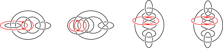
Figure 31. The configuration of the type $\mathrm{II}^{3}$ singular fibers.

Appendix A Hyperbolic structures

Let $P$ be a (branched) shadow of a $3$-manifold $M$, and let $c$ be a component of $S(P)$. Set $P^{\prime}:=\operatorname{Nbd}(c;P)$. It is easily seen that if $c$ contains no vertices of $P$, $\pi_{P}^{-1}(P^{\prime})$ is a pair of pants bundle over $S^{1}$. In particular, $\pi_{P}^{-1}(P^{\prime})$ is a Seifert fibered space in this case. Suppose that $c$ contains $n$ vertices of $P$, where $n>0$. In this case, it was shown by Costantino-Thurston [3, Proposition 3.33] that $\operatorname{Int}\pi_{P}^{-1}(P^{\prime})$ is a hyperbolic manifold of volume $2nv_{\mathrm{oct}}$. In fact, for each vertex in $c$, we can construct two ideal regular octahedra glued together along some of their faces to form a handlebody of genus three, and the remaining faces are glued together using the combinatorial structure along the edges of $P^{\prime}$. See also Ishikawa-Koda [8, Section 6].

Let $X(P)$ be the set of local parts of $P$ homeomorphic to $X$ depicted in Figure 9 whose vertices are contained in $c$. Recall that a branched shadow obtained as in Theorem 2.1 always contains this type of local part, each of which corresponds to a singular fiber of type $\mathrm{II}^{3}$. Suppose that $X(P)\neq\emptyset$, and $X(P)=\{X_{1},X_{2},\ldots,X_{m}\}$. Set $P^{\prime\prime}:=P^{\prime}\cup\bigcup_{i}X_{i}$. Then it was mentioned in Costantino-Thurston [3, Theorem 3.38] that $\operatorname{Int}\pi_{P}^{-1}(P^{\prime\prime})$ admits a hyperbolic structure of volume $2(n-2m)v_{\mathrm{oct}}+10mv_{\mathrm{ted}}$. In fact, we can show that for each vertex in $P^{\prime\prime}-P^{\prime}$, we can construct two ideal regular octahedra glued together as above, and for each $X_{i}$, we can construct ten ideal regular tetrahedra glued together along some of their faces to form a handlebody of genus three. Then the remaining faces, all of them are totally geodesic ideal regular triangles, are glued together using the combinatorial structure along the edges of $P^{\prime\prime}$. We believe it is worth giving an explicit description of this fact here. The following proposition is essential and enough to see that.

Proposition A.1.

Let $P_{1}$ be the shadowed polyhedron illustrated in Figure 21 equipped with the coloring of $\partial P_{1}$ by $\partial_{e}(P_{1})=\partial P_{1}$. Let $M$ be the compact $3$-manifold represented by $P_{1}$. Then $\operatorname{Int}M$ is a hyperbolic $3$-manifold that admits a decomposition into ten ideal regular tetrahedra. Further, let $Y_{1}$ and $Y_{2}$ be the cones over three points in $P_{1}$ that cut $P_{1}$ into $X$. Then $\pi_{P_{1}}^{-1}(Y_{i})\cap\operatorname{Int}M$ $(i=1,2)$ is a totally geodesic open pair of pants consisting of two faces of those ideal tetrahedra.

Proof.

As we have seen in the proof of Theorem 0.1, $M=E(L_{1}^{\prime})$. By Dunfield-Thurston [5], the complement of $L^{\prime}_{1}$ can be decomposed into ten ideal regular tetrahedra as follows.

Let $\tau:E(L^{\prime}_{1})\to E(L^{\prime}_{1})$ be the involution as shown in Figure 32.

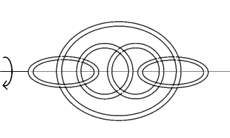
Figure 32. The involution $\tau$.

Consider the double branched cover $E(L^{\prime}_{1})\to E(L^{\prime}_{1})/\tau$. We think of $S^{3}$ as the boundary of the $4$-simplex $\Delta^{4}$. Then as shown in Figure 33, $E(L^{\prime}_{1})/\tau$ is homeomorphic to the boundary of $\Delta^{4}$ minus an open ball neighborhood of each vertex of $\Delta^{4}$, and the image of the set of fixed points of $\tau$ corresponds to the set of edges of $\Delta^{4}$.

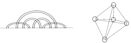
Figure 33. The quotient space $E(L^{\prime}_{1})/\tau$.

In this way, we obtain a decomposition of $E(L^{\prime}_{1})/\tau$ into five truncated tetrahedra such that each edge is touched by three faces. This decomposition lifts to a decomposition of $E(L^{\prime}_{1})$ into truncated tetrahedra whose dihedral angles are all $\pi/3$. Thus, this induces a decomposition of $\operatorname{Int}M$ into ten ideal regular hyperbolic tetrahedra.

The preimages $\pi_{P_{1}}^{-1}(Y_{1})$ and $\pi_{P_{1}}^{-1}(Y_{2})$ of $Y_{1}$ and $Y_{2}$ are pair of pants as shown in Figure 34.

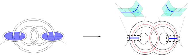
Figure 34. The preimages $\pi_{P_{1}}^{-1}(Y_{1})$ and $\pi_{P_{1}}^{-1}(Y_{2})$.

Each of those pair of pants consists of exactly two faces of the truncated tetrahedra constructed above. Thus, $\pi_{P_{1}}^{-1}(Y_{i})\cap\operatorname{Int}M$ $(i=1,2)$ is a totally geodesic open pair of pants consisting of two faces of the above ideal regular tetrahedra. ∎

As we have seen in Claim 1 of the proof of Theorem 0.1, the polyhedra $P_{2},P_{3},P_{4}$ illustrated in Figure 21 are all obtained by cutting $P_{1}$ along $Y_{1}\cup Y_{2}$ and then re-gluing the cut ends appropriately. Thus, we have the following.

Corollary A.2.

The links $L_{1}^{\prime},L_{2}^{\prime},L_{3}^{\prime},L_{4}^{\prime}\subset S^{3}$ in Figure 2 are all hyperbolic of volume $10v_{\mathrm{tet}}$.

By the proof of Proposition A.1, we also have the following.

Corollary A.3.

The cusp shapes of the complements of the hyperbolic links $L_{1}^{\prime},L_{2}^{\prime},L_{3}^{\prime},L_{4}^{\prime}\subset S^{3}$ in Figure 2 are as shown in Figure 35.

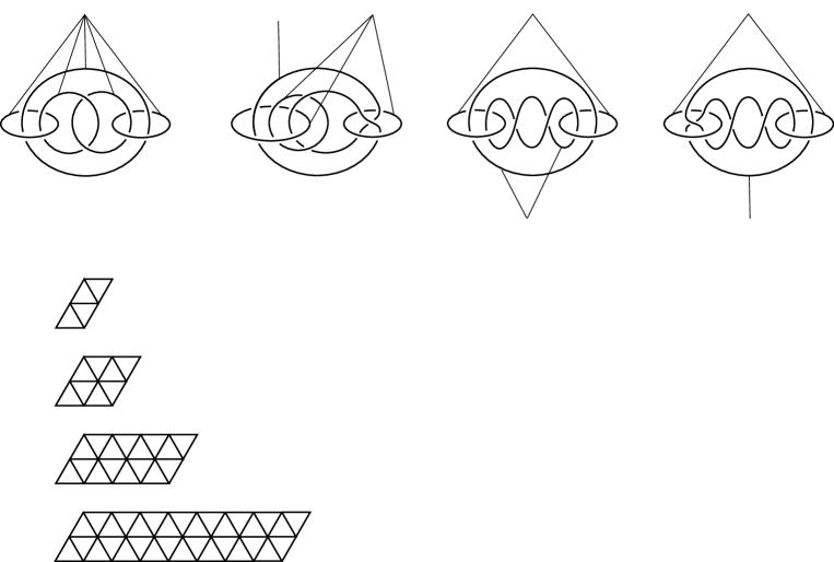
Figure 35. The cusp shapes of the complements of $L_{1}^{\prime},L_{2}^{\prime},L_{3}^{\prime},L_{4}^{\prime}$.

References

- [1] Burlet, O., de Rham, G., Sur certaines applications génériques d’une variété close à 3 dimensions dans le plan, Enseignement Math. (2) 20 (1974), 275–292.
- [2] Costantino, F., Shadows and branched shadows of and -manifolds, Edizioni della Normale, Scuola Normale Superiore, Pisa, Italy, 2005.
- [3] Costantino, F., Thurston, D., 3-manifolds efficiently bound 4-manifolds, J. Topol. 1(3), pp. 703–745 (2008).
- [4] Culler, M., Dunfield, N. M., Goerner, M., Weeks, J. R., SnapPy, a computer program for studying the geometry and topology of -manifolds, available at http://snappy.computop.org.
- [5] Dunfield, N., Thurston, W.P., The virtual Haken conjecture: experiments and examples, Geom. Topol. 7, pp. 399–441 (2003).
- [6] Golubitsky, M., Guillemin, V., Stable mappings and their singularities, Graduate Texts in Mathematics, Vol. 14, Springer-Verlag, New York-Heidelberg, 1973.
- [7] Gromov, M., Singularities, expanders and topology of maps. I. Homology versus volume in the spaces of cycles, Geom. Funct. Anal. 19 (2009), no. 2, 743–841.
- [8] Ishikawa, M., Koda, Y., Stable maps and branched shadows of 3-manifold, Math. Ann. 367, pp. 1819–1863 (2017).
- [9] Kalmár, B., Stipsicz, A. I., Maps on 3-manifolds given by surgery, Pacific J. Math. 257 (2012), no. 1, 9–35.
- [10] Kushner, L., Levine, H., Porto, P., Mapping three-manifolds into the plane. I, Bol. Soc. Mat. Mexicana (2) 29 (1984), no. 1, 11–33.
- [11] Levine, H., Elimination of cusps, Topology 3, suppl. 2, pp. 263–296 (1965).
- [12] Levine, H., Classifying immersions into over stable maps of -manifolds into , Lecture Notes in Mathematics 1157, Springer-Verlag, Berlin, 1985.
- [13] Mather, J., Stability of mappings, VI: The nice dimensions, Proceedings of Liverpool Singularities-Symposium, I, Lecture Notes in Math., Vol. 192, Springer, Berlin, pp. 207–253 (1971).
- [14] Saeki, O., Stable maps and links in 3-manifolds, Workshop on Geometry and Topology (Hanoi, 1993), Kodai Math. J. 17 (1994), no. 3, 518–529.
- [15] Saeki, O., Simple stable maps of 3-manifolds into surfaces, Topology 35(3), pp. 671–698 (1996).
- [16] Saeki, O., Topology of singular fibers of differentiable maps, Lecture Notes in Mathematics, 1854, Springer-Verlag, Berlin, 2004.
- [17] Turaev, V.G., Shadow links and face models of statistical mechanics, J. Differential Geom. 36(1), pp. 35–74 (1992).
- [18] Turaev, V.G., Quantum invariants of knots and -manifolds, de Gruyter Studies in Mathematics, vol. 18. Walter de Gruyter & Co., Berlin (1994).