Using contrastive learning to improve the performance of steganalysis schemes

Abstract.

To improve the detection accuracy and generalization of steganalysis, this paper proposes the Steganalysis Contrastive Framework (SCF) based on contrastive learning. The SCF improves the feature representation of steganalysis by maximizing the distance between features of samples of different categories and minimizing the distance between features of samples of the same category. To decrease the computing complexity of the contrastive loss in supervised learning, we design a novel Steganalysis Contrastive Loss (StegCL) based on the equivalence and transitivity of similarity. The StegCL eliminates the redundant computing in the existing contrastive loss. The experimental results show that the SCF improves the generalization and detection accuracy of existing steganalysis DNNs, and the maximum promotion is 2% and 3% respectively. Without decreasing the detection accuracy, the training time of using the StegCL is 10% of that of using the contrastive loss in supervised learning.

1. Introduction

Steganography generates the stego by embedding undetectable messages into the cover and makes them as close in distribution as possible (Wu et al., 2019; Pevnỳ et al., 2010). Steganalysis is to detect whether an object is a cover or a stego (Zhang et al., 2019; Wang et al., 2018; Cogranne et al., 2019).

According to the development history of steganalysis, steganalysis is divided into traditional steganalysis and DNN-based steganalysis. The traditional steganalysis scheme is to design handcrafted features followed by a classifier. The most classical traditional steganalysis scheme is the Rich Model (Fridrich and Kodovsky, 2012) followed by an Ensemble Classifier (Kodovsky et al., 2011). Recently, most steganalysis schemes are based on the DNN. Qian et al. (Qian et al., 2015) unify the feature extraction and classification two steps under a single DNN. XuNet (Xu et al., 2016) facilitates the hyperbolic tangent (TanH) activation function and $1\times 1$ convolutional kernel. YeNet (Ye et al., 2017) utilizes the optimizable filters of Spatial Rich Model (SRM) (Fridrich and Kodovsky, 2012) as the preprocessing module. Yedroudj et al. (Yedroudj et al., 2018) introduce the batch normalization and non-linear activation function. Fridrich et al. (Boroumand et al., 2018) propose an end-to-end DNN called SRNet that introduces shortcut operation (Szegedy et al., 2017). Zhao et al. (You et al., 2020) put forward a novel DNN with the siamese architecture. These DNN-based steganalysis schemes propose kinds of structures to optimize the DNN. The structures maximize the distance between features of cover and stego, which improves the detection accuracy of steganalysis. Taking the similarity between samples of the same category into account, this paper introduces contrastive learning to minimize the distance between features of samples of the same category and maximize the distance between features of samples of different categories, which improves the detection accuracy and generalization of steganalysis DNNs.

The main contributions of this paper can be summarized as follows:

• To improve the detection accuracy and generalization of steganalysis, this paper proposes a Steganalysis Contrastive Framework (SCF) based on contrastive learning. The SCF improves the feature representation of steganalysis by maximizing the distance between features of samples of different categories, and minimizing the distance between features of samples of the same category.

• To decrease the computing complexity of supervised contrastive loss (Khosla et al., 2020), we design a novel Steganalysis Contrastive Loss (StegCL) based on the equivalence and transitivity of similarity. Without decreasing the detection accuracy, the StegCL eliminates the redundant computing in the contrastive loss in supervised learning.

The rest of the paper is organized as follows: in Section II, the DNN-based steganalysis and the loss of contrastive learning are introduced, in Section III, the SCF and the StegCL are explained, in Section IV, there are the setups of the experiments and the experimental results, and Section V summarizes the paper.

2. Background

2.1. DNN-based steganalysis

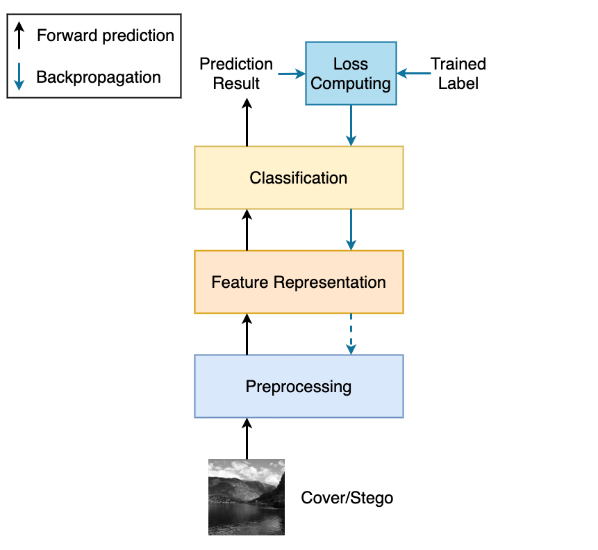
Figure 1. The basic framework of existing steganalysis DNNs.

The basic framework of existing steganalysis DNNs is shown in Figure 1. There is the preprocessing module, feature representation module, and classification module in the framework. The preprocessing module filters the input image to obtain the high-frequency information of the image. The feature representation module extracts the high-dimensional features of the filtered image. The classification module classifies the high-dimensional features and obtains the prediction result. The black arrows indicate the process of forwarding prediction. During the forwarding prediction, the input image goes through preprocessing, feature representation, and classification modules in turn. The output of the forwarding prediction is the prediction result. The blue arrows indicate the process of backpropagation. During the backpropagation, the loss computing module computes the cross-entropy loss (Zhang and Sabuncu, 2018) with the prediction result and the trained label. Then, the computed loss is utilized by the backpropagation to update the parameters of the DNN. The dashed arrow between the feature representation module and the preprocessing module means that sometimes the parameters of the preprocessing module are not updated (Xu et al., 2016).

Existing DNN-based steganalysis works focus on optimizing the preprocessing module and the feature representation module. To optimize the preprocessing module, Xu et al. (Xu et al., 2016) put forward to utilizing the fixed filters of SRM (Denemark et al., 2014). Ye et al. (Ye et al., 2017) propose that the parameters of filters of SRM need to be updated. Fridrich et al. (Boroumand et al., 2018) utilize a convolution layer, a batch normalization layer, and a ReLU layer with default initialization as the preprocessing module. To optimize the feature representation module, Yedroudj et al. (Yedroudj et al., 2018) design a non-linear activation function called truncation function that maximizes the small difference between cover and stego. SRNet (Boroumand et al., 2018) introduces the shortcut operation (Szegedy et al., 2017), which extracts more residual information between cover and stego. Zhao et al. (You et al., 2020) put forward KeNet with a novel siamese architecture according to the left and right imbalance of the difference between cover and stego. These works propose kinds of schemes to optimize the preprocessing module and the feature representation module. The schemes maximize the difference between features of cover and stego, which improves the detection accuracy of steganalysis. Inspired by contrastive learning that greatly improves the feature representation in CV and NLP (Chen et al., 2020b, a; Jaiswal et al., 2021), this paper proposes the Steganalysis Contrastive Framework (SCF) based on contrastive learning to improve the performance of steganalysis schemes.

2.2. The loss of contrastive learning

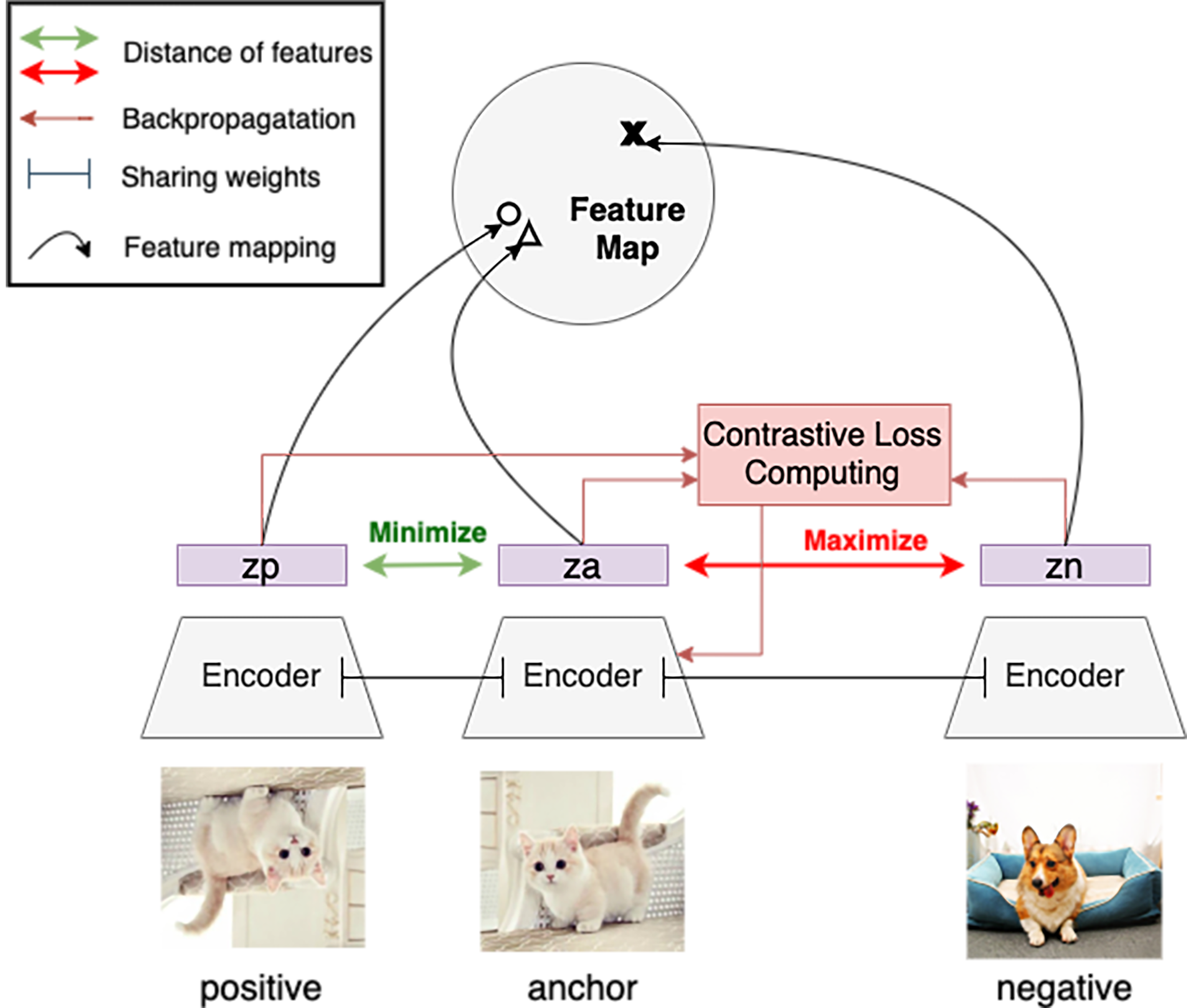
Figure 2. The basic principle of contrastive learning.

The target of contrastive learning is to minimize the distance between features of the anchor and the positive, and maximize the distance between features of the anchor and the negative. The basic principle of contrastive learning is shown in Figure 2. The three Encoders have the same structures and parameters. The $za$, $zp$, and $zn$ are the features extracted from the anchor, the positive, and the negative by the Encoder. The contrastive loss computing module computes the contrastive loss with the $za$, $zp$, and $zn$. The contrastive loss used by the backpropagation is the core of contrastive learning. As the backpropagation updates the parameters of the Encoder to decrease the contrastive loss, the $za$ and $zp$ gradually approach, and the $za$ and $zn$ gradually move away from each other, which achieves the target of contrastive learning. There are mainly two kinds of contrastive loss: Self-supervised Contrastive Loss (SelfCL) (Chen et al., 2020b, a; Jaiswal et al., 2021) and Supervised Contrastive Loss (SupCL) (Khosla et al., 2020).

(1) $$\mathbb{L}^{self}=\sum^{2N}_{i=1}\mathbb{L}^{self}_{i}$$

(2) $$\mathbb{L}^{self}_{i}=-\log{\frac{\exp(z_{i}\cdot z_{j(i)}/\tau)}{\sum^{2N}_{k=1}\ell_{i\neq k}\cdot\exp(z_{i}\cdot z_{k}/\tau)}}$$

The SelfCL is used in self-supervised learning (Jaiswal et al., 2021; Chen et al., 2020b, a), In self-supervised learning, because of the lack of the labels of samples, the contrast occurs between the anchor, the augmentation of the anchor (the positive), and the samples different from the anchor (the negative). The SelfCL aims at maximizing the distance between features of the anchor and the samples different from the anchor, and minimizing the distance between features of the anchor and the augmentation. The calculation of SelfCL is shown in Formula 1 and 2. Formula 1 indicates that the total SelfCL of a batch is the sum of the loss of each sample. Formula 2 shows how to calculate the loss of each sample. The $z_{i}$, $z_{j(i)}$, $z_{k}$ refers to the features extracted from the anchor, the positive, and the negative. The value of $\mathbb{L}^{self}_{i}$ represents the negative logarithm of the proportion of Euclidean Distances (Danielsson, 1980) of $z_{i}$ and $z_{j(i)}$ to the sum of Euclidean Distances of $z_{i}$ and all $z_{k}$. Decreasing the value of $\mathbb{L}^{self}_{i}$ increases the proportion of Euclidean Distance of $z_{i}$ and $z_{j(i)}$ to the sum of Euclidean Distances of $z_{i}$ and all $z_{k}$, which makes the feature of the anchor similar to the feature of the augmentation, and makes the feature of the anchor different from all features of other samples. The SelfCL greatly promotes the development of contrastive learning, however, the SelfCL doesn’t introduce the label and there is only one positive by default. The SelfCL is unavailable in supervised learning, and cannot be utilized by the steganalysis schemes.

(3) $$\mathbb{L}^{sup}=\sum^{2N}_{i=1}\mathbb{L}^{sup}_{i}$$

(4) $$\mathbb{L}^{sup}_{i}=\frac{-1}{2N_{\widetilde{y}_{i}}-1}\sum^{2N}_{j=1}\ell_{i\neq j}\cdot\ell_{\widetilde{y}_{i}=\widetilde{y}_{j}}\cdot\log{\frac{\exp(z_{i}\cdot z_{j}/\tau)}{\sum^{2N}_{k=1}\ell_{i\neq k}\cdot\exp(z_{i}\cdot z_{k}/\tau)}}$$

Recently, Google researchers propose the Supervised Contrastive Loss (SupCL) to introduce contrastive learning into supervised learning in NeurIPS 2020 (Khosla et al., 2020). The SupCL takes the labels of samples into account and contrasts the anchor with more than one positive. With the help of the labels, the contrast occurs between the anchor, the samples whose labels are the same as that of the anchor (the positive), and the samples whose labels are different from that of the anchor (the negative). The SupCL tries to bring the features of samples of the same category close, and keep the features of samples of different categories far away. The calculation of SupCL is shown in Formula 3 and 4. Compared to the $\mathbb{L}^{self}_{i}$ shown in Formula 2, the $\mathbb{L}^{sup}_{i}$ can be understood as the normalized sum of $(2N_{\widetilde{y}_{i}}-1)$ times $\mathbb{L}^{self}_{i}$ computing, and each $\mathbb{L}^{self}_{i}$ makes the anchor similar to the only one positive. By $(2N_{\widetilde{y}_{i}}-1)$ times $\mathbb{L}^{self}_{i}$ computing, the anchor is similar to all samples of the same category.

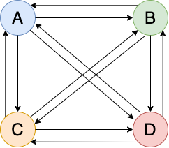
(a) $4\times 3$ times computing

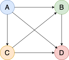
(b) $4\times 3\div 2$ times computing

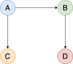
(c) $3$ times computing

Figure 3. The three schemes to make samples (A, B, C, and D) of the same category similar. The black arrow represents once $\mathbb{L}^{self}_{i}$ computing.

There is redundant computing in the SupCL. To make it easier for readers to understand, Figure 3 is drawn to explain the redundant computing in the SupCL. Three schemes make $N=4$ samples of the same category similar. Figure 3 (a) represents the scheme used by the SupCL, which has $N\times(N-1)=12$ times $\mathbb{L}^{self}_{i}$ computing. Figure 3 (b) represents the scheme that removes the repeat computing ($A\rightarrow B$ is repeated to $B\rightarrow A$ ), and there are $N\times(N-1)\div 2=6$ times computing. The scheme in Figure 3 (c) considers the transitivity of similarity( $A\rightarrow B$ and $B\rightarrow C$, which makes $A\rightarrow C$ unnecessary), and there is $N-1=3$ times computing left. All schemes in Figure 3 can make samples of the same category similar. However, the scheme used by the SupCL needs more computing, which means that the contrastive loss in supervised learning has redundant computing.

3. Proposed methods

Based on the analysis above, we propose the Steganalysis Contrastive Framework (SCF) that introduces contrastive learning into steganalysis for the first time. To eliminate the redundant computing in the existing contrastive loss, a novel Steganalysis Contrastive Loss (StegCL) is designed based on the equivalence and transitivity of similarity.

3.1. Steganalysis Contrastive Framework

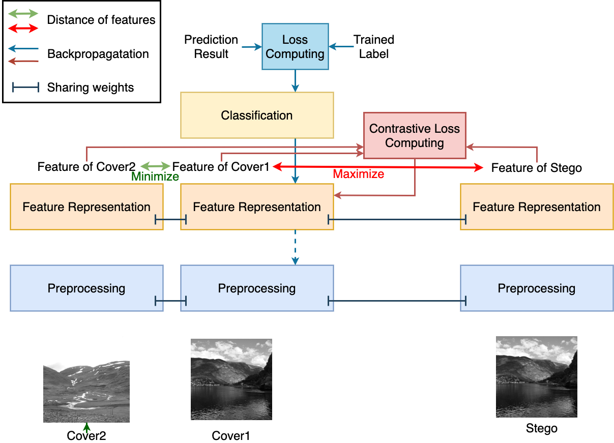
Figure 4. The architecture of the SCF.

The architecture of the Steganalysis Contrastive Framework (SCF) is shown in Figure 4. The main difference between the SCF and the basic framework of existing steganalysis DNNs (seen in Figure 1) is that the SCF adds a contrastive loss computing module. This module computes the contrastive loss with the features extracted by the feature representation module. The SCF retains the backpropagation from the loss computed with the prediction result and the trained label, which maximizes the distance between features of cover and stego. Meanwhile, the SCF introduces a new backpropagation from the contrastive loss, which not only maximizes the distance between features of cover and stego but also minimizes the distance between features of samples of the same category.

3.2. Steganalysis Contrastive Loss

(5) $$\mathbb{L}^{steg}=\sum^{2N}_{i=1}\mathbb{L}^{steg}_{i}$$

(6) $$\mathbb{L}^{steg}_{i}=-\log{\frac{\exp({z_{i}}\cdot z_{j(Random\cdot\ell_{(i)\neq(j)}\cdot\ell_{\widetilde{y}_{i}=\widetilde{y}_{j}})}/\tau)}{\sum^{2N}_{k=1}\ell_{i\neq k}\cdot\ell_{\widetilde{y}_{i}\neq\widetilde{y}_{j}}\cdot\exp(z_{i}\cdot z_{k}/\tau)}}$$

The Steganalysis Contrastive Loss (StegCL) is shown in Formula 5 and 6. Compared to the $\mathbb{L}^{sup}_{i}$ shown in Formula 4, the $\mathbb{L}^{steg}_{i}$ only contains once $\mathbb{L}^{self}_{i}$ computing. The advantage of the StegCL is that it minimizes the features of samples of the same category without redundant computing. The core of the StegCL is the Random Selection Strategy (RSS) that is the $(Random\cdot\ell_{(i)\neq(j)}\cdot\ell_{\widetilde{y}_{i}=\widetilde{y}_{j}})$ shown in Formula 6. The RSS selects the same category sample in different set of the anchor as the positive. Algorithm 1 presents how the RSS works. To make it easier for readers to understand, Figure 5 is drawn to explain how Algorithm 1 executes when there are 4 samples of the same category. Figure 5 (a) shows that samples are not similar to each other at the start. Figure 5 (b) shows that anchor A select sample D as the positive, which makes A similar to D and merges the sets. Figure 5 (c) shows that anchor B select sample C as the positive, which makes B similar to C and merges the sets. Figure 5 (d) shows that anchor C select sample D as the positive, which makes the A, B, C and D are similar to each other and merges the sets. With the help of the RSS used in StegCL, each anchor only need to be similar to one positive, and the samples of the same category are similar to each other finally.

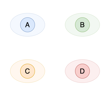
(a) Initialization

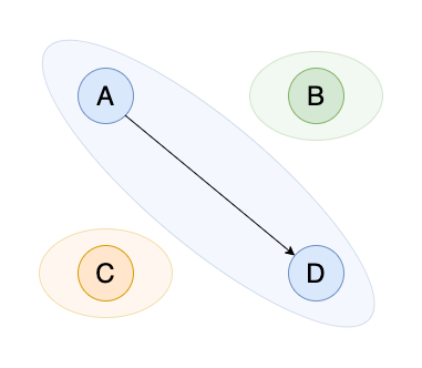
(b) $A\rightarrow D$

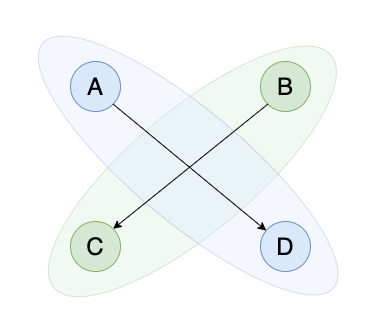
(c) $B\rightarrow C$

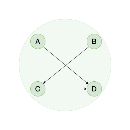
(d) $C\rightarrow D$

Figure 5. The figures explain how Algorithm1 works. The A, B, C, and D in the circle are the samples of the same category. The ellipses are the sets that contain the same category samples. The arrow means once $\mathbb{L}^{self}_{i}$ computing.

1

input : A batch $Im$ of $N$ number

output : None

2

3U $\leftarrow$ SetFunction($Im[1:N]$);

4 for $i\leftarrow 1$ to $N$ do

5       set $\leftarrow$ SetFunction($Im[i]$);

6      

7 end for

8

9for $i\leftarrow 1$ to $N-1$ do

10       set $\leftarrow$ GetElementSet($Im[i]$);

11       set $\leftarrow$ U $-$ set ;

12       image $\leftarrow$ RandomSelectFromSet(set);

13       MakeClose($Im[i]$ and image);

14       UnionSetFunction($Im[i]$ and image);

15      

16 end for

17

Algorithm 1 The algorithm that utilizes RSS to make samples of the same category similar. The RSStrategy is the red part.

4. Experiments

To analyze the performance of the SCF and the StegCL, the detection accuracy, generalization, and computing complexity are evaluated. To evaluate the detection accuracy, the DNNs optimized with the SCF are tested on WOW (Holub and Fridrich, 2012), S-UNIWARD (Holub et al., 2014), and MiPOD (Sedighi et al., 2015) at $0.2$ bpp and $0.4$ bpp payloads, and the results are compared to that of the original DNNs without the optimization of the SCF. To evaluate the generalization, the detection accuracy of the optimized DNNs is compared to that of the original DNNs in case of mismatch. To evaluate the computing complexity, the StegCL and the SupCL are used by the SCF, and the training time is compared. The details of the experiment are as follows.

4.1. Setups

4.1.1. Dataset

The dataset used in experiments is BOSSbase $1.01$ (Bas et al., 2011) which contains $10,000$ Portable GrayMap format images. These images are $512\times 512$ pixels. Considering that the GPU used in experiments is GeForce $2080$Ti that has merely $12$G memory, these images are resized to $256\times 256$ pixels by the imresize function in MATLAB with default settings. For simplification, the dataset with resized images is called BOSSbase256. The images in BOSSbase256 are used as covers in experiments. To generate the stegoes from the covers, four self-adaptive steganography algorithms, HUGO (Pevnỳ et al., 2010), WOW (Holub and Fridrich, 2012), S-UNIWARD (Holub et al., 2014), MiPOD (Sedighi et al., 2015) are facilitated. There are $0.1$ bpp, $0.2$ bpp, $0.3$ bpp, and $0.4$ bpp four payloads in experiments. S-UNIWARD $0.4$ bpp BOSSbase256 represents the dataset that contains $10,000$ covers and $10,000$ stegoes generated by S-UNIWARD (Holub et al., 2014) at $0.4$ bpp payload. Each dataset is randomly divided into three parts in a ratio of $6$:$1$:$3$ for training, validation, and testing.

4.1.2. Metric

The performance of detection accuracy is measured with the total classification error probability on the test subset of the dataset under equal priors $P_{E}$$=\min_{P_{FA}}\frac{1}{2}(P_{FA}+P_{MD})$ (Boroumand et al., 2018; You et al., 2020; Yedroudj et al., 2018; Ye et al., 2017), where $P_{FA}$ and $P_{MD}$ are the false-alarm and missed-detection probabilities.

4.2. Experimental designs

4.2.1. Evaluation of detection accuracy

The $P_{E}$ of original DNNs and DNNs optimized with the SCF are compared on different datasets. With WOW (Holub and Fridrich, 2012), S-UNIWARD (Holub et al., 2014), and MiPOD (Sedighi et al., 2015) at $0.2$ bpp and $0.4$ bpp, six different datasets are constructed. YeNet (Ye et al., 2017), YedroudjNet (Yedroudj et al., 2018), KeNet (You et al., 2020), CL-YeNet, CL-YedroudjNet, and CL-KeNet are trained and tested on these datasets. The $P_{E}$ of the DNNs are compared.

4.2.2. Evaluation of generalization

Steganography Algorithm Mismatch

The DNNs are trained on algorithm known datasets and tested on algorithm unknown datasets. HUGO (Pevnỳ et al., 2010), WOW (Holub and Fridrich, 2012), S-UNIWARD (Holub et al., 2014), MiPOD (Sedighi et al., 2015), $0.4$ bpp BOSSbase256 are constructed. KeNet (You et al., 2020) and CL-KeNet are trained on one of these datasets and tested on all four datasets. Meanwhile, the $P_{E}$ of KeNet and CL-KeNet are compared with each other.

Payload Mismatch

The DNNs are trained on payload known datasets and tested on payload unknown datasets. S-UNIWARD (Holub et al., 2014) $0.1$ bpp, $0.2$ bpp, $0.3$ bpp, $0.4$ bpp BOSSbase256 are constructed. KeNet (You et al., 2020) and CL-KeNet are trained on one of these datasets and tested on all four datasets. Meanwhile, the $P_{E}$ of KeNet and CL-KeNet are compared with each other.

4.2.3. Comparation of computing complexity between StegCL and SupCL (Khosla et al., 2020)

The SupCL-KeNet (KeNet+SCF+SupCL (Khosla et al., 2020)), KeNet (You et al., 2020), and StegCL-KeNet (KeNet+SCF+StegCL) are trained and tested on S-UNIWARD $0.4$ bpp BOSSbase256. The training time and the $P_{E}$ of the DNNs are compared.

4.3. Experimental results

4.3.1. Evaluation of detection accuracy

The line graphs of $P_{E}$ are shown in Figure 6. The horizontal axis represents steganography algorithms, and the vertical axis indicates the detection error rates $P_{E}$. The dashed lines represent the $P_{E}$ of YeNet (Ye et al., 2017), YedroudjNet (Yedroudj et al., 2018), and KeNet (You et al., 2020). The solid lines represent the $P_{E}$ of CL-YeNet, CL-KeNet, and CL-YedroudjNet. The solid lines are lower than the dashed lines with the same color, which means that the detection accuracy is improved with the help of the SCF. The detailed experimental results are shown in Table 1. The $P_{E}$ of the DNNs optimized with the SCF is $0.5\%$ to $3\%$ lower than that of the original DNNs, which means the SCF increases the detection accuracy of steganalysis.

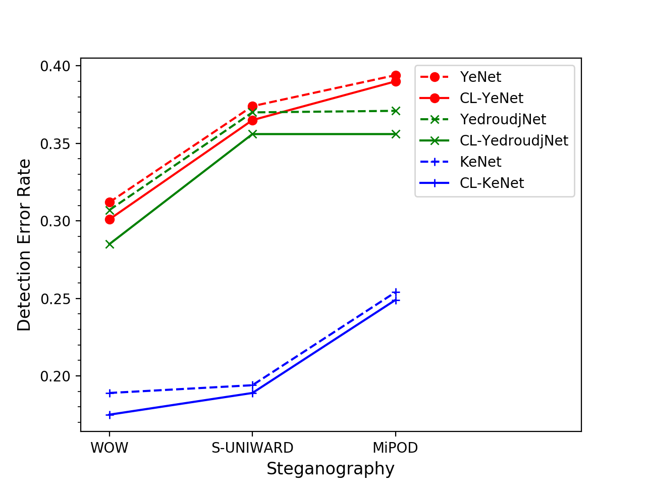
(a) 0.2 bpp

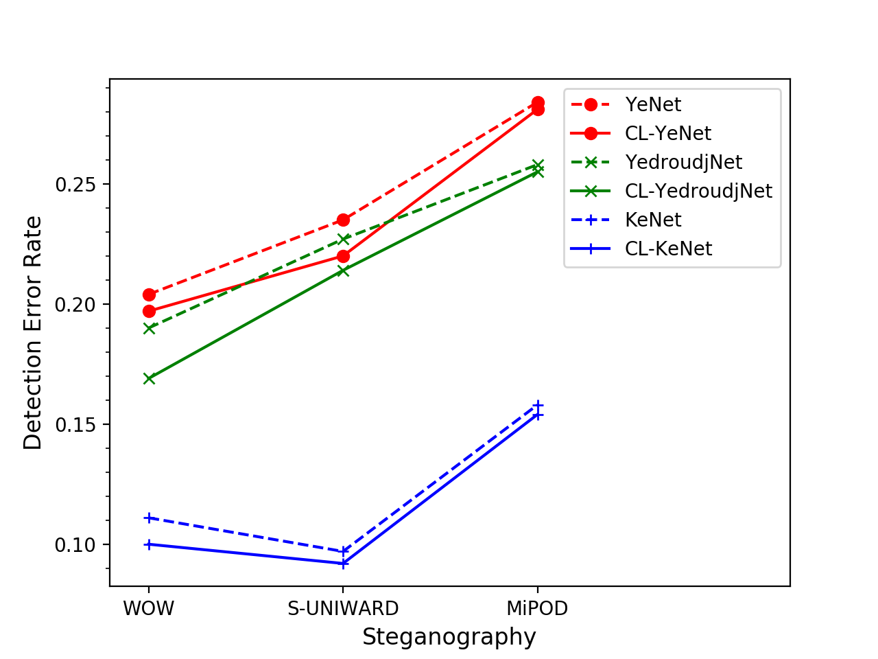
(b) 0.4 bpp

Figure 6. The line graphs that represent the $\boldsymbol{P_{E}}$ of YeNet (Ye et al., 2017), CL-YeNet, YedroudjNet (Yedroudj et al., 2018), CL-YedroudjNet, KeNet (You et al., 2020), and CL-KeNet on WOW (Holub and Fridrich, 2012), S-UNIWARD (Holub et al., 2014), MiPOD (Sedighi et al., 2015) at 0.2 bpp and 0.4 bpp.

Table 1. The $\boldsymbol{P_{E}}$ of YeNet (Ye et al., 2017), CL-YeNet, YedroudjNet (Yedroudj et al., 2018), CL-YedroudjNet, KeNet (You et al., 2020), and CL-KeNet on WOW (Holub and Fridrich, 2012), S-UNIWARD (Holub et al., 2014), MiPOD (Sedighi et al., 2015) at 0.2 bpp and 0.4 bpp.

Steganography	WOW (Holub and Fridrich, 2012)		S-UNIWARD (Holub et al., 2014)		MiPOD (Sedighi et al., 2015)
Payload	0.2 bpp	0.4 bpp	0.2 bpp	0.4 bpp	0.2 bpp	0.4 bpp
YeNet (Ye et al., 2017)	.312	.204	.374	.235	.394	.284
CL-YeNet	.301	.197	.365	.220	.390	.281
YedroudjNet (Yedroudj et al., 2018)	.307	.190	.370	.227	.371	.258
CL-YedroudjNet	.285	.169	.356	.214	.356	.255
KeNet (You et al., 2020)	.189	.111	.194	.097	.254	.158
CL-KeNet	.175	.100	.189	.092	.249	.154

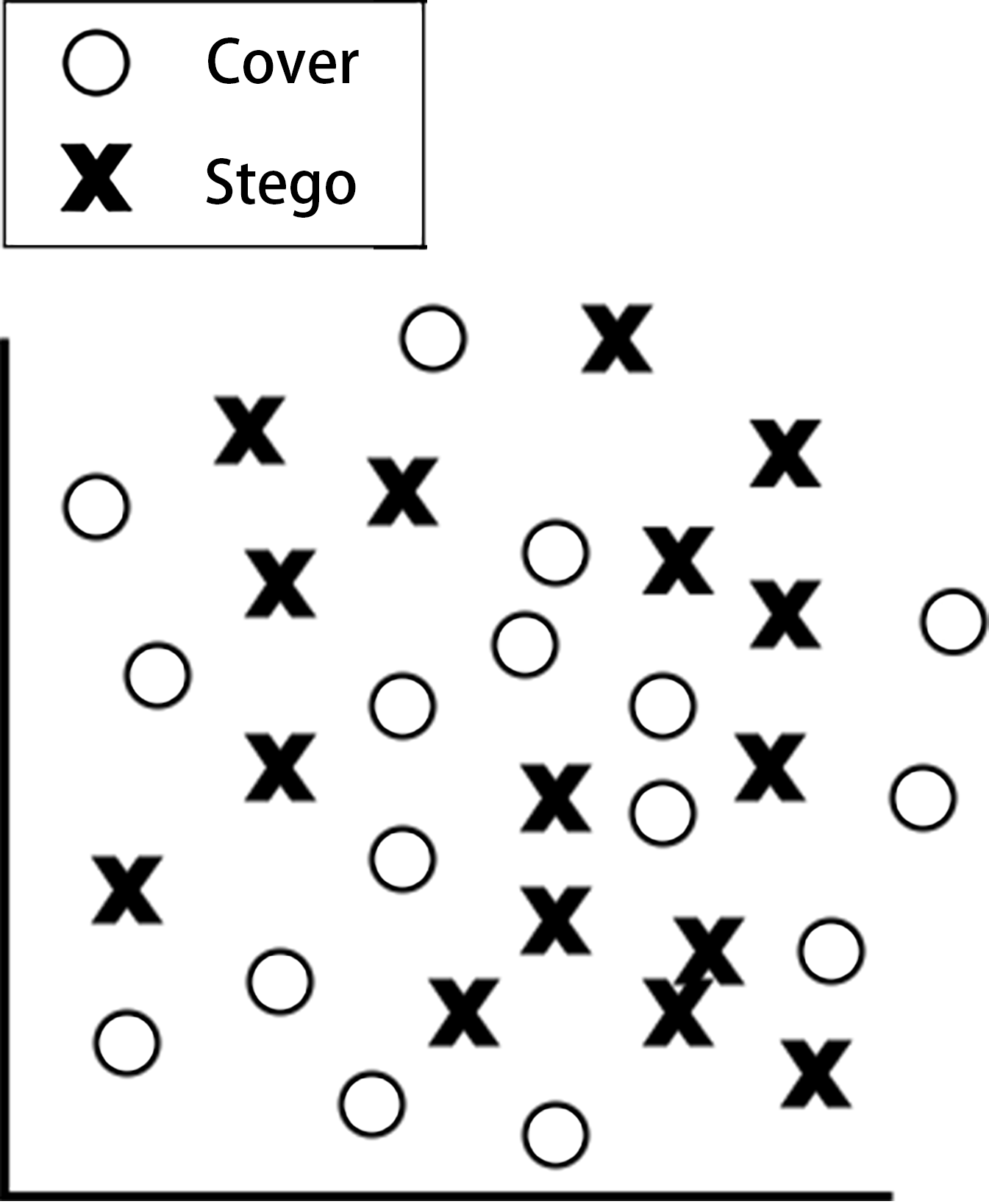
(a) from KeNet (You et al., 2020)

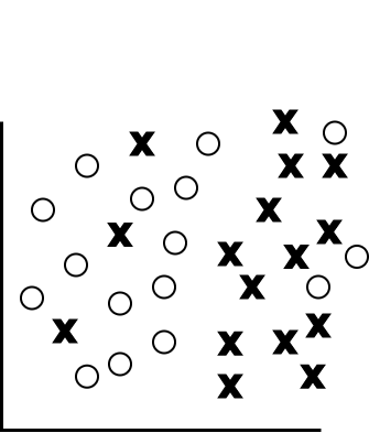
(b) from CL-KeNet

Figure 7. The 2-D t-SNE features

The Feature Representation Modules (FRMs) of KeNet (You et al., 2020) and CL-KeNet are utilized to extract the features. Two batch features are extracted from the same batch samples by the FRMs. Then the features are reduced to $2$-Dimensions with t-SNE (Maaten and Hinton, 2008). These $2$-D features are plotted in two axes in Figure 7. The features in Figure 7 (b) are more discriminating than those in Figure 7 (a), which means the SCF minimizes the distance between features of samples of the same category.

4.3.2. Evaluation of generalization

Table 2. The $\boldsymbol{P_{E}}$ of KeNet (You et al., 2020) and CL-KeNet in case of steganography algorithm mismatch under the same 0.4 bpp payload.

MODELS	TRA $\backslash$ TES	WOW (Holub and Fridrich, 2012)	HUGO (Pevnỳ et al., 2010)	S-UNI* (Holub et al., 2014)	MiPOD (Sedighi et al., 2015)
KeNet (You et al., 2020)	WOW (Holub and Fridrich, 2012)	.110	.383	.205	.289
CL-KeNet		.100	.378	.191	.287
KeNet	HUGO (Pevnỳ et al., 2010)	.318	.174	.321	.320
CL-KeNet		.302	.153	.311	.308
KeNet	S-UNI* (Holub et al., 2014)	.106	.276	.097	.214
CL-KeNet		.101	.268	.092	.211
KeNet	MiPOD (Sedighi et al., 2015)	.150	.262	.167	.158
CL-KeNet		.149	.250	.154	.153

Table 3. The $\boldsymbol{P_{E}}$ of KeNet (You et al., 2020) and CL-KeNet in case of payload mismatch under the same S-UNIWARD (Holub et al., 2014) steganography algorithm.

MODELS	TRA $\backslash$ TES	0.1 bpp	0.2 bpp	0.3 bpp	0.4 bpp
KeNet (You et al., 2020)	0.1 bpp	.382	.254	.215	.174
CL-KeNet		.375	.248	.212	.153
KeNet	0.2 bpp	.395	.238	.160	.158
CL-KeNet		.393	.230	.148	.153
KeNet	0.3 bpp	.400	.281	.153	.110
CL-KeNet		.399	.279	.139	.100
KeNet	0.4 bpp	.442	.302	.203	.097
CL-KeNet		.431	.298	.200	.092

The $P_{E}$ of KeNet (You et al., 2020) and CL-KeNet in case of mismatch is shown in Table 2 and Table 3. Table 2 shows the $P_{E}$ in case of steganography algorithm mismatch. When the DNN is trained on one steganography and tested on HUGO (Pevnỳ et al., 2010), WOW (Holub and Fridrich, 2012), S-UNIWARD (Holub et al., 2014) and MiPOD (Sedighi et al., 2015), the $P_{E}$ of CL-KeNet are all lower than that of KeNet (You et al., 2020), which represents that the SCF improves the generalization of steganalysis DNNs when steganography algorithm mismatch happens. Table 3 shows the $P_{E}$ in case of payload mismatch. The $P_{E}$ of CL-KeNet are whole lower than that of KeNet (You et al., 2020) when the DNN is trained on one payload and tested on four payloads, which means that the SCF improves the generalization of steganalysis DNNs when payload mismatch happens.

4.3.3. Comparation of computing complexity between StegCL and SupCL (Khosla et al., 2020)

Table 4. The Training time of each epoch and $\boldsymbol{P_{E}}$ of KeNet (You et al., 2020), SupCL-KeNet, and StegCL-KeNet on the S-UNIWARD 0.4 bpp BOSSbase256.

MODELS	Training time of each epoch	$\boldsymbol{P_{E}}$
KeNet (You et al., 2020)	170 seconds	.0979
SupCL (Khosla et al., 2020)-KeNet	2100 seconds	.0926
StegCL-KeNet	200 seconds	.0921

Table 4 shows the training time and $P_{E}$ of KeNet (You et al., 2020), SupCL-KeNet, and StegCL-KeNet. In the column of training time of each epoch, the values of KeNet (You et al., 2020) and StegCL-KeNet are close, but the value of SupCL-KeNet is far from that of these. The $P_{E}$ of StegCL-KeNet is smaller than that of SupCL-KeNet. The experimental result shows that the designed StegCL costs less training time than that of the contrastive loss in supervised learning, without decreasing the detection accuracy.

5. Conclusion

This paper introduces contrastive learning into steganalysis for the first time and proposes the Steganalysis Contrastive Framework (SCF). The SCF is utilized to optimize well-known steganalysis DNNs, YeNet, YedroudjNet, and KeNet. The experimental results indicate that contrastive learning can greatly improve the detection accuracy and generalization of existing steganalysis DNNs. Meanwhile, we optimize the contrastive loss in supervised learning and design a novel StegCL based on the equivalence and transitivity of similarity. The StegCL eliminates the redundant computing in the contrastive loss in supervised learning and reduces the computing complexity. The future work will further follow the idea of contrastive learning, mining the intrinsic correlation of cover and stego to improve the performance of the steganalysis schemes.

References

- (1)
- Bas et al. (2011) Patrick Bas, Tomáš Filler, and Tomáš Pevnỳ. 2011. ” Break our steganographic system”: the ins and outs of organizing BOSS. In International workshop on information hiding. Springer, 59–70.
- Boroumand et al. (2018) Mehdi Boroumand, Mo Chen, and Jessica Fridrich. 2018. Deep residual network for steganalysis of digital images. IEEE Transactions on Information Forensics and Security 14, 5 (2018), 1181–1193.
- Chen et al. (2020b) Ting Chen, Simon Kornblith, Mohammad Norouzi, and Geoffrey Hinton. 2020b. A simple framework for contrastive learning of visual representations. arXiv preprint arXiv:2002.05709 (2020).
- Chen et al. (2020a) Xinlei Chen, Haoqi Fan, Ross Girshick, and Kaiming He. 2020a. Improved baselines with momentum contrastive learning. arXiv preprint arXiv:2003.04297 (2020).
- Cogranne et al. (2019) Rémi Cogranne, Quentin Giboulot, and Patrick Bas. 2019. The alaska steganalysis challenge: A first step towards steganalysis. In Proceedings of the ACM Workshop on Information Hiding and Multimedia Security. 125–137.
- Danielsson (1980) Per-Erik Danielsson. 1980. Euclidean distance mapping. Computer Graphics and image processing 14, 3 (1980), 227–248.
- Denemark et al. (2014) Tomas Denemark, Vahid Sedighi, Vojtech Holub, Rémi Cogranne, and Jessica Fridrich. 2014. Selection-channel-aware rich model for steganalysis of digital images. In 2014 IEEE International Workshop on Information Forensics and Security (WIFS). IEEE, 48–53.
- Fridrich and Kodovsky (2012) Jessica Fridrich and Jan Kodovsky. 2012. Rich models for steganalysis of digital images. IEEE Transactions on Information Forensics and Security 7, 3 (2012), 868–882.
- Holub and Fridrich (2012) Vojtěch Holub and Jessica Fridrich. 2012. Designing steganographic distortion using directional filters. In 2012 IEEE International workshop on information forensics and security (WIFS). IEEE, 234–239.
- Holub et al. (2014) Vojtěch Holub, Jessica Fridrich, and Tomáš Denemark. 2014. Universal distortion function for steganography in an arbitrary domain. EURASIP Journal on Information Security 2014, 1 (2014), 1–13.
- Jaiswal et al. (2021) Ashish Jaiswal, Ashwin Ramesh Babu, Mohammad Zaki Zadeh, Debapriya Banerjee, and Fillia Makedon. 2021. A survey on contrastive self-supervised learning. Technologies 9, 1 (2021), 2.
- Khosla et al. (2020) Prannay Khosla, Piotr Teterwak, Chen Wang, Aaron Sarna, Yonglong Tian, Phillip Isola, Aaron Maschinot, Ce Liu, and Dilip Krishnan. 2020. Supervised contrastive learning. arXiv preprint arXiv:2004.11362 (2020).
- Kodovsky et al. (2011) Jan Kodovsky, Jessica Fridrich, and Vojtěch Holub. 2011. Ensemble classifiers for steganalysis of digital media. IEEE Transactions on Information Forensics and Security 7, 2 (2011), 432–444.
- Maaten and Hinton (2008) Laurens van der Maaten and Geoffrey Hinton. 2008. Visualizing data using t-SNE. Journal of machine learning research 9, Nov (2008), 2579–2605.
- Pevnỳ et al. (2010) Tomáš Pevnỳ, Tomáš Filler, and Patrick Bas. 2010. Using high-dimensional image models to perform highly undetectable steganography. In International Workshop on Information Hiding. Springer, 161–177.
- Qian et al. (2015) Yinlong Qian, Jing Dong, Wei Wang, and Tieniu Tan. 2015. Deep learning for steganalysis via convolutional neural networks. In Media Watermarking, Security, and Forensics 2015, Vol. 9409. International Society for Optics and Photonics, 94090J.
- Sedighi et al. (2015) Vahid Sedighi, Rémi Cogranne, and Jessica Fridrich. 2015. Content-adaptive steganography by minimizing statistical detectability. IEEE Transactions on Information Forensics and Security 11, 2 (2015), 221–234.
- Szegedy et al. (2017) Christian Szegedy, Sergey Ioffe, Vincent Vanhoucke, and Alexander Alemi. 2017. Inception-v4, inception-resnet and the impact of residual connections on learning. In Proceedings of the AAAI Conference on Artificial Intelligence, Vol. 31.
- Wang et al. (2018) Yuntao Wang, Kun Yang, Xiaowei Yi, Xianfeng Zhao, and Zhoujun Xu. 2018. CNN-based steganalysis of MP3 steganography in the entropy code domain. In Proceedings of the 6th ACM Workshop on Information Hiding and Multimedia Security. 55–65.
- Wu et al. (2019) Songtao Wu, Sheng-hua Zhong, and Yan Liu. 2019. A novel convolutional neural network for image steganalysis with shared normalization. IEEE Transactions on Multimedia 22, 1 (2019), 256–270.
- Xu et al. (2016) Guanshuo Xu, Han-Zhou Wu, and Yun-Qing Shi. 2016. Structural design of convolutional neural networks for steganalysis. IEEE Signal Processing Letters 23, 5 (2016), 708–712.
- Ye et al. (2017) Jian Ye, Jiangqun Ni, and Yang Yi. 2017. Deep learning hierarchical representations for image steganalysis. IEEE Transactions on Information Forensics and Security 12, 11 (2017), 2545–2557.
- Yedroudj et al. (2018) Mehdi Yedroudj, Frédéric Comby, and Marc Chaumont. 2018. Yedroudj-net: An efficient CNN for spatial steganalysis. In 2018 IEEE International Conference on Acoustics, Speech and Signal Processing (ICASSP). IEEE, 2092–2096.
- You et al. (2020) Weike You, Hong Zhang, and Xianfeng Zhao. 2020. A Siamese CNN for Image Steganalysis. IEEE Transactions on Information Forensics and Security 16 (2020), 291–306.
- Zhang et al. (2019) Ru Zhang, Feng Zhu, Jianyi Liu, and Gongshen Liu. 2019. Depth-wise separable convolutions and multi-level pooling for an efficient spatial CNN-based steganalysis. IEEE Transactions on Information Forensics and Security 15 (2019), 1138–1150.
- Zhang and Sabuncu (2018) Zhilu Zhang and Mert Sabuncu. 2018. Generalized cross entropy loss for training deep neural networks with noisy labels. Advances in neural information processing systems 31 (2018), 8778–8788.