An introduction to finite element methods for inverse coefficient problems in elliptic PDEs

Abstract

Several novel imaging and non-destructive testing technologies are based on reconstructing the spatially dependent coefficient in an elliptic partial differential equation from measurements of its solution(s). In practical applications, the unknown coefficient is often assumed to be piecewise constant on a given pixel partition (corresponding to the desired resolution), and only finitely many measurement can be made. This leads to the problem of inverting a finite-dimensional non-linear forward operator $\mathcal{F}:\ \mathcal{D}(\mathcal{F})\subseteq\mathbb{R}^{n}\to\mathbb{R}^{m}$, where evaluating $\mathcal{F}$ requires one or several PDE solutions.

Numerical inversion methods require the implementation of this forward operator and its Jacobian. We show how to efficiently implement both using a standard FEM package and prove convergence of the FEM approximations against their true-solution counterparts. We present simple example codes for Comsol with the Matlab Livelink package, and numerically demonstrate the challenges that arise from non-uniqueness, non-linearity and instability issues. We also discuss monotonicity and convexity properties of the forward operator that arise for symmetric measurement settings.

This text assumes the reader to have a basic knowledge on Finite Element Methods, including the variational formulation of elliptic PDEs, the Lax-Milgram-theorem, and the Céa-Lemma. Section 3 also assumes that the reader is familiar with the concept of Fréchet differentiability.

1 Introduction

Many practical reconstruction problems in the field of medical imaging and non-destructive testing lead to inverse coefficient problems in elliptic partial differential equations. This text is meant to be an introductory tutorial for implementing such problems with Finite Element Methods (FEM).

We assume that the unknown coefficient is piecewise-constant on a given resolution, and that finitely many linear measurements of one of several solutions are taken, where different solutions are generated by different linear excitation in the underlying physics model. This leads to the finite-dimensional non-linear inverse problem of determining

$$\sigma\in\mathbb{R}^{n}\quad\text{ from }\quad\mathcal{F}(\sigma)\in\mathbb{R}^{m}$$

with $n\in\mathbb{N}$ unknowns and $m\in\mathbb{N}$ measurements.

Iterative numerical solution methods for this inverse problem require evaluating $\mathcal{F}$ and its derivatives at each iteration step, which means solving the underlying elliptic PDE. In this work, we will demonstrate how FEM-based implementations for $\mathcal{F}$ and its Jacobian can be obtained very efficiently from standard FEM-solvers for the considered elliptic PDE. Roughly speaking, the sensitivity of a measurement with respect to changing the coefficient in one pixel can be simply calculated by multiplying FEM-solutions corresponding to the measurement and excitation patterns with so-called pixel stiffness matrices that are obtained from summing up all element stiffness matrices of elements belonging to the pixel where the change occurs. Hence, the FEM-based Jacobian can be obtained without any additional computational burden with just a few lines of extra code. Alternatively, for an even simpler implementation, the pixel stiffness matrices can be easily obtained by subtracting global stiffness matrices without requiring any knowledge about the triangulation details.

This text is meant as a simple-to-read explanation of this approach in a sufficiently general but naturally arising setting. More precisely, we restrict ourselves to coercive and symmetric variational formulations that linearly depend on the unknown coefficients, and to excitations and measurements that correspond to linear functionals. In this setting, we demonstrate how to obtain the Jacobian of the FEM-based forward map with the means of a standard FEM software package such as COMSOL. We also discuss monotonicity and convexity properties arising in symmetric measurement situations that are the basis for recent research on rigorously justified reconstruction methods.

The purpose of this text is of introductory nature, but we proceed in a mathematically rigorous fashion to allow this text to also serve as a reference. We prove differentiability of the true-solution forward operator and its FEM-based approximation, and show convergence of the FEM-approximated quantities to their true-solution counterparts.

Section 2 gives two examples to motivate our general setting: stationary diffusion and Elecrical Impedance Tomography. Section 3 introduces the forward operator using the exact PDE solution and derives its properties. The FEM-approximation of the forward operator and its Jacobian is studied in section 4. In section 5 we show numerical examples and demonstrate some of the major challenges that arise in solving inverse coefficient problems. The COMSOL/MATLAB source codes for all examples are given in appendix A.

2 Motivation and examples

2.1 Stationary diffusion

We consider the stationary diffusion equation

$$-\nabla\cdot(\sigma\nabla u)=g\quad\text{ in $\Omega$}$$ (1)

with homogeneous Dirichlet boundary condition $u|_{\partial\Omega}=0$ in a Lipschitz bounded domain $\Omega\subset\mathbb{R}^{d}$, $d\in\mathbb{N}$. For $u\in H^{1}(\Omega)$, $\sigma\in L^{\infty}_{+}(\Omega)$ and $g\in L^{2}(\Omega)$ the equation is equivalent to finding $u\in H_{0}^{1}(\Omega)$ with

$$\int_{\Omega}\sigma\nabla u\cdot\nabla v\,{\rm{d}}x=\int_{\Omega}gv\,{\rm{d}}x\quad\text{ for all }v\in H_{0}^{1}(\Omega),$$ (2)

and unique solvability follows from the Lax-Milgram theorem.

We are interested in the inverse coefficient problem of determining the diffusivity coefficient $\sigma$ in (1) from measurements of the solution for one or several source terms $g$, cf. hanke1997regularizing for an application in groundwater filtration. In practical applications with finitely many measurements, it is natural to only aim for a certain pixel-based resolution and therefore assume that $\sigma$ is piecewise constant with respect to a partition $\Omega=\bigcup_{i=1}^{n}\mathcal{P}_{i}$, i.e.

$$\sigma(x)=\sum_{i=1}^{n}\sigma_{i}\chi_{\mathcal{P}_{i}}(x)\quad\text{ for all }x\in\Omega,$$

where the pixels $\mathcal{P}_{i}\subseteq\Omega$ are assumed to be measurable subsets. The left image in figure 1 shows a simple example where the unit square $\Omega=(0,1)^{2}$ is divided into $3\times 3$ pixels. In the following, with a slight abuse of notation, we write $\sigma=(\sigma_{1},\ldots,\sigma_{n})^{T}\in\mathbb{R}^{n}$ for the unknown diffusivity.

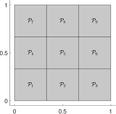
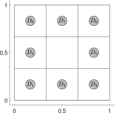
Figure 1: Pixel partition and circular subdomains used for excitations and measurements.

The source term $g$ in the diffusion model (1) can be identified with the linear functional on the right hand side of the variational formulation (2)

$$l\in H^{-1}(\Omega),\quad l(v):=\int_{\Omega}gv\,{\rm{d}}x,$$

which corresponds to identifying $L^{2}(\Omega)$ with a subset of $H^{-1}(\Omega)$. Accordingly, we consider excitations in the form of linear functionals. Also, to emphasize that the solution depends on the diffusion coefficient and the excitation, we write $u_{\sigma}^{l}$ in the following. The left image in figure 2 illustrates the concentration resulting from a constant source term $g=\chi_{D}$, i.e. $l(v)=\int_{D}v\,{\rm{d}}x$, where $D=D_{2}\cup D_{4}\cup D_{5}\cup D_{7}$ is a union of four circular subdomains as sketched in the right image of figure 1. The right image in figure 2 shows the corresponding plot for $D=D_{1}\cup D_{3}\cup D_{6}\cup D_{8}$. Both images show the solution of (1) with constant diffusion coefficient $\sigma=1$.

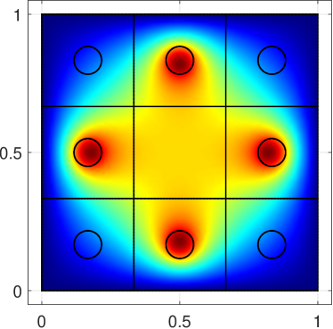
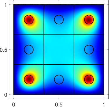
Figure 2: PDE solution for source terms on circular subdomains.

Natural models for measuring the solution of (1) also yield to linear functionals. Measuring the total concentration in one of the circular subdomains $D_{j}$ corresponds to measuring $r(u):=\int_{D_{j}}u\,{\rm{d}}x$. Hence, the inverse problem of determining finitely many information about the diffusivity coefficient from finitely many measurements of the concentration (possibly but not necessarily resulting from different excitations) leads to the finite-dimensional inverse problem to

$$\text{determine}\quad\sigma\in\mathbb{R}^{n}_{+}\quad\text{ from }\quad\mathcal{F}(\sigma)\in\mathbb{R}^{m},$$

where

$$\mathcal{F}:\ \mathbb{R}^{n}_{+}\to\mathbb{R}^{m},\quad\mathcal{F}(\sigma):=(r_{j}(u_{\sigma}^{l_{j}}))_{j=1}^{m},$$

and $u_{\sigma}^{l_{j}}\in H_{0}^{1}(\Omega)$ solves

$$\sum_{i=1}^{n}\sigma_{i}b_{i}(u_{\sigma}^{l_{j}},v)=l_{j}(v)\quad\text{ for all }v\in H_{0}^{1}(\Omega),$$

with given $l_{j},r_{j}\in H^{-1}(\Omega)$, $j=1,\ldots,m$, and

$$b_{i}(u,v):=\int_{\mathcal{P}_{i}}\nabla u\cdot\nabla v\,{\rm{d}}x,\quad i=1,\ldots,n.$$

2.2 Electrical Impedance Tomography (EIT)

We give another example for an application that leads to an inverse elliptic coefficient problems in a similar form as the diffusion example.

EIT aims to image the inner conductivity structure of a subject by current and voltage measurements through electrodes attached to the imaging subject. Let $\Omega\subseteq\mathbb{R}^{d}$, $d\in\{2,3\}$, be a smoothly bounded domain denoting the imaging subject. The electrodes $\mathcal{E}_{k}$, $k=1,\ldots,K$, are assumed to be open connected subsets of $\partial\Omega$ with disjoint closures.

When currents with strength $J=(J_{1},\ldots,J_{K})\in\mathbb{R}^{K}$ are driven through the $K$ electrodes (with $\sum_{k=1}^{K}J_{k}=0$), the resulting electric potential $u\in H^{1}(\Omega)$ inside $\Omega$, and the potential $U\in\mathbb{R}^{K}$ on the electrodes, solve

$$\nabla\cdot(\sigma\nabla u) =0\quad \text{ in }\Omega,$$

$$\sigma\partial_{\nu}u =0\quad \text{ on }\partial\Omega\setminus\bigcup_{k=1}^{K}\mathcal{E}_{k},$$

$$u+z\sigma\partial_{\nu} u=\text{const.}=:U_{k}\quad \text{ on }\mathcal{E}_{k},\ k=1,\ldots,K,$$

$$\int_{\mathcal{E}_{k}}\sigma\partial_{\nu}|_{\mathcal{E}_{k}}\,{\rm{d}}s =J_{k} \text{ on }\mathcal{E}_{k},\ k=1,\ldots,K,$$

where $\sigma\in L^{\infty}_{+}(\Omega)$ is the conductivity inside $\Omega$, and $z>0$ is the contact impedance of the electrodes.

Under the gauge condition $U\in\mathbb{R}_{\diamond}^{K}:=\{V\in\mathbb{R}^{K}:\ \sum_{k=1}^{K}V_{k}=0\}$, one can show (see somersalo1992existence ) that this so-called complete electrode model (CEM) for EIT is equivalent to the variational formulation that $(u,U)\in H^{1}(\Omega)\times\mathbb{R}^{K}_{\diamond}$ solves

$$\int_{\Omega}\sigma\nabla u\cdot\nabla w\,{\rm{d}}x+\sum_{k=1}^{K}\int_{\mathcal{E}_{k}}\frac{1}{z}(u-U_{k})(w-W_{k})\,{\rm{d}}s=\sum_{k=1}^{K}J_{k}W_{k}$$ (3)

for all $(w,W)\in H^{1}(\Omega)\times\mathbb{R}^{K}_{\diamond}$, and unique solvability follows from the Lax-Milgram theorem.

We assume that $z>0$ is known, and that $\sigma(x)=\sum_{i=1}^{n}\sigma_{i}\chi_{\mathcal{P}_{i}}(x)$ is piecewise constant with respect to a pixel partition $\Omega=\bigcup_{i=1}^{n}\mathcal{P}_{i}$, and write $\sigma=(\sigma_{1},\ldots,\sigma_{n})\in\mathbb{R}^{n}$ for the unknown conductivity values inside $\Omega$.

The applied current patterns $J=(J_{1},\ldots,J_{K})\in\mathbb{R}^{K}$ can be identified with the functional

$$l\in H^{\prime},\quad l(w,W):=\sum_{k=1}^{K}J_{k}W_{k}\quad\text{ for all }(w,W)\in H:=H^{1}(\Omega)\times\mathbb{R}^{K}_{\diamond}.$$

Likewise, measuring the voltage between the $k_{1}$-th and the $k_{2}$-th electrode corresponds to measuring the linear functional

$$r\in H^{\prime},\quad r(u,U):=U_{k_{1}}-U_{k_{2}},$$

of the solution $(u,U)\in H$ generated by some current pattern.

Hence, the problem of determining the interior conductivity with a fixed finite resolution from finitely many voltage-current measurements in EIT (with CEM) leads to the finite-dimensional inverse problem to

$$\text{determine}\quad\sigma\in\mathbb{R}^{n}_{+}\quad\text{ from }\quad\mathcal{F}(\sigma)\in\mathbb{R}^{m},$$

where $\mathcal{F}:\ \mathbb{R}^{n}_{+}\to\mathbb{R}^{m},\quad\mathcal{F}(\sigma):=(r_{j}(u_{\sigma}^{l_{j}},U_{\sigma}^{l_{j}}))_{j=1}^{m}$, and $(u_{\sigma}^{l_{j}},U_{\sigma}^{l_{j}})\in H$ solves

$$b_{0}((u_{\sigma}^{l_{j}},U_{\sigma}^{l_{j}}),(w,W))+\sum_{i=1}^{n}\sigma_{i}\,b_{i}((u_{\sigma}^{l_{j}},U_{\sigma}^{l_{j}}),(w,W))=l_{j}(w,W)$$

for all $(w,W)\in H$, with given $l_{j},r_{j}\in H^{\prime}$, $j=1,\ldots,m$, and

$$b_{0}((u,U),(w,W)) :=\sum_{k=1}^{K}\int_{\mathcal{E}_{k}}\frac{1}{z}(u-U_{k})(w-W_{k})\,{\rm{d}}s,$$

$$b_{i}((u,U),(w,W)) :=\int_{\mathcal{P}_{i}}\nabla u\cdot\nabla w\,{\rm{d}}x.$$

Clearly, one could also extend this formulation to cover the case of unknown contact impedances.

3 The true-solution setting

The examples in section 2 lead to inverse problems for a finite-dimensional non-linear forward operator $\mathcal{F}:\ \mathbb{R}^{n}_{+}\to\mathbb{R}^{m}$, where evaluations of $\mathcal{F}$ require solving an infinite-dimensional linear problem (the PDE). In this section, we will first derive some properties of $\mathcal{F}$ for the case that it is defined with the true infinite-dimensional PDE solution. The properties of the operator $F\approx\mathcal{F}$, that is defined with a FEM-approximation of the PDE solution, will be studied in section 4.

3.1 The true-solution forward operator and its derivative

We will study problems that appear in the variational formulation of elliptic PDEs with piecewise constant coefficients on a fixed pixel partition, as in the examples in section 2.

The variational setting.

Let $H$ be a Hilbert space. We consider the problem of finding $u\in H$ that solves

$$b_{\sigma}(u,v)=l(v),$$ (4)

where $b_{\sigma}:\ H\times H\to\mathbb{R}$ is a bilinear form, and $l\in H^{\prime}=\mathcal{L}(H,\mathbb{R})$. $b_{\sigma}$ is assumed to linearly depend on $n$ parameters $\sigma=(\sigma_{1},\ldots,\sigma_{n})\in\mathbb{R}^{n}$ in the following way

$$b_{\sigma}(u,v)=b_{0}(u,v)+\sum_{i=1}^{n}\sigma_{i}b_{i}(u,v),$$

where $b_{0},\ b_{i}:\ H\times H\to\mathbb{R}$ are bounded, symmetric and positive semidefinite bilinear forms. Writing $\mathbbm{1}:=(1,\ldots,1)^{T}\in\mathbb{R}^{n}$, we also assume that $b_{\mathbbm{1}}$ is bounded and coercive with constants $\beta,C>0$, i.e.,

$$C\hskip 0.86108pt\|v\|\hskip 0.86108pt^{2}\geq b_{\mathbbm{1}}(v,v)=b_{0}(v,v)+\sum_{i=1}^{n}b_{i}(v,v)\geq\beta\hskip 0.86108pt\|v\|\hskip 0.86108pt^{2}\quad\forall v\in H.$$

Clearly, this yields that for all $\sigma\in\mathbb{R}^{n}_{+}$

$$C\max\{1,\sigma_{1},\ldots,\sigma_{n}\}\hskip 0.86108pt\|v\|\hskip 0.86108pt^{2}\geq b_{\sigma}(v,v)\geq\beta\min\{1,\sigma_{1},\ldots,\sigma_{n}\}\hskip 0.86108pt\|v\|\hskip 0.86108pt^{2}\quad\forall v\in H,$$ (5)

so that $b_{\sigma}$ is symmetric, bounded and coercive. Here and in the following $\mathbb{R}^{n}_{+}$ denotes the set of all $\sigma\in\mathbb{R}^{n}$ with $\sigma>0$ and ”$>$” and ”$\geq$” are understood elementwise on $\mathbb{R}^{n}$.

The true-solution forward operator.

We now characterize the derivative of the solution of (4) with respect to $\sigma$.

Lemma 1

Let $l\in H^{\prime}$. The solution operator

$$\mathcal{S}:\ \mathbb{R}^{n}_{+}\to H,\quad\mathcal{S}(\sigma):=u_{\sigma}^{l},\quad\text{ where $u_{\sigma}^{l}\in H$ solves \eqref{eq:varform},}$$

is infinitely often Fréchet differentiable. Its first derivative

$$S^{\prime}:\ \mathbb{R}^{n}_{+}\to\mathcal{L}(\mathbb{R}^{n},H)$$

fulfills that, for all $\sigma\in\mathbb{R}^{n}_{+}$ and $\tau\in\mathbb{R}^{n}$, $S^{\prime}(\sigma)\tau\in H$ is the unique solution of

$$b_{\sigma}(S^{\prime}(\sigma)\tau,w)=-\sum_{i=1}^{n}\tau_{i}b_{i}(u_{\sigma}^{l},w)\quad\forall w\in H.$$

Also, for $r\in H^{\prime}$, $\sigma\in\mathbb{R}^{n}_{+}$, and $\tau\in\mathbb{R}^{n}$,

$$r(u_{\sigma}^{l})=b_{\sigma}(u_{\sigma}^{l},u_{\sigma}^{r})\quad\text{ and }\quad r\left(\mathcal{S}^{\prime}(\sigma)\tau\right)=-\sum_{i=1}^{n}\tau_{i}b_{i}(u_{\sigma}^{l},u_{\sigma}^{r}).$$

Proof

For $\sigma\in\mathbb{R}^{n}_{+}$, the Riesz theorem yields that there exists a unique operator $\mathcal{B}(\sigma)\in\mathcal{L}(H,H^{\prime})$ associated to the bilinear form $b_{\sigma}(\cdot,\cdot)$, i.e.

$$\langle\mathcal{B}(\sigma)u,v\rangle_{H^{\prime}\times H}=b_{\sigma}(u,v)\quad\text{ for all }u,v\in H.$$

Clearly, $\mathcal{B}(\sigma)$ is symmetric and, by the Lax-Milgram theorem, $\mathcal{B}(\sigma)$ is invertible with symmetric inverse $\mathcal{B}(\sigma)^{-1}\in\mathcal{L}(H^{\prime},H)$. Hence, (4) is uniquely solvable, and the solution operator $\mathcal{S}$ is well-defined.

It is easily checked, that $\mathcal{B}(\sigma)$ is Fréchet differentiable for every $\sigma\in\mathbb{R}^{n}_{+}$, and that its derivative $\mathcal{B}^{\prime}(\sigma)\in\mathcal{L}(\mathbb{R}^{n},\mathcal{L}(H,H^{\prime}))$ is given by

$$\mathcal{B}^{\prime}(\sigma)\tau=\sum_{i=1}^{n}\tau_{i}\mathcal{B}_{i}\quad\text{ for all }\sigma\in\mathbb{R}^{n}_{+},\ \tau\in\mathbb{R}^{n},$$

where $\mathcal{B}_{i}\in\mathcal{L}(H,H^{\prime})$ is the unique operator fulfilling

$$(\mathcal{B}_{i}u,v)_{H^{\prime}\times H}=b_{i}(u,v)\quad\text{ for all }u,v\in H.$$

Since $\mathcal{B}^{\prime}(\sigma)$ does not depend on $\sigma$, this also shows that $\mathcal{B}(\sigma)$ is infinitely often Fréchet differentiable with all second and higher derivatives being zero.

Using the derivative of operator inversion and the product and chain rule for the Fréchet derivative, we thus obtain that $\mathcal{S}(\sigma)$ is infinitely often Fréchet differentiable with

$$\mathcal{S}^{\prime}(\sigma)\tau =-\mathcal{B}(\sigma)^{-1}(\mathcal{B}^{\prime}(\sigma)(\tau))\mathcal{B}(\sigma)^{-1}l=-\sum_{i=1}^{n}\tau_{i}\mathcal{B}(\sigma)^{-1}\mathcal{B}_{i}u_{\sigma}^{l}.$$

Hence, $v=\mathcal{S}^{\prime}(\sigma)\tau\in H$ solves

$$b_{\sigma}(v,w) =-\sum_{i=1}^{n}\langle\tau_{i}\mathcal{B}_{i}u_{\sigma}^{l},w\rangle_{H^{\prime}\times H}=-\sum_{i=1}^{n}\tau_{i}b_{i}(u_{\sigma}^{l},w)\quad\forall w\in H.$$

Moreover, we obtain for all $r\in H^{\prime}$, by using the symmetry of $\mathcal{B}(\sigma)$,

$$r(u_{\sigma}^{l})=\langle\mathcal{B}(\sigma)\mathcal{B}(\sigma)^{-1}r,u_{\sigma}^{l}\rangle_{H^{\prime}\times H}=b_{\sigma}(u_{\sigma}^{l},u_{\sigma}^{r}),$$

and

$$r\left(\mathcal{S}^{\prime}(\sigma)\tau\right) =\langle r,\mathcal{S}^{\prime}(\sigma)\tau\rangle_{H^{\prime}\times H}=\langle\mathcal{B}(\sigma)\mathcal{S}^{\prime}(\sigma)\tau,\mathcal{B}(\sigma)^{-1}r\rangle_{H^{\prime}\times H}$$

$$=-\sum_{i=1}^{n}\tau_{i}\langle\mathcal{B}_{i}\,u_{\sigma}^{l},u_{\sigma}^{r},\rangle_{H^{\prime}\times H}=-\sum_{i=1}^{n}\tau_{i}b_{i}(u_{\sigma}^{l},u_{\sigma}^{r}),$$

which finished the proof. $\Box$

Corollary 1

Let $l,r\in H^{\prime}$. Then the mapping

$$\mathcal{F}_{l,r}:\ \mathbb{R}^{n}_{+}\to\mathbb{R},\quad\mathcal{F}_{l,r}(\sigma):=r(u_{\sigma}^{l})$$

fulfills

$$\mathcal{F}_{l,r}(\sigma)=b_{\sigma}(u_{\sigma}^{l},u_{\sigma}^{r})\quad\text{ for all $\sigma\in\mathbb{R}^{n}_{+}$.}$$

Moreover, $\mathcal{F}_{l,r}:\ \mathbb{R}^{n}_{+}\to\mathbb{R}$ is infinitely often differentiable and its first derivatives fulfill

$$\frac{\partial}{\partial\sigma_{i}}\mathcal{F}_{l,r}(\sigma)=-b_{i}(u_{\sigma}^{l},u_{\sigma}^{r}).$$

Proof

This follows from Lemma 1. $\Box$

3.2 Convexity and monotonicity for symmetric measurements

A special mathematical structure appears for measurements $\mathcal{F}_{l,r}$, when $l$ and $r$ are taken from the same subset of $H^{\prime}$, and all combinations are used. In the stationary diffusion example this corresponds to using the same subsets of $\Omega$ both for excitations and concentration measurements, in EIT this corresponds to using the same electrodes for voltage and current measurements.

Given a set of $m\in\mathbb{N}$ excitations/measurements $\{l_{1},\ldots,l_{m}\}\subset H^{\prime}$, we combine the measurements into a matrix-valued map $\mathcal{F}:\ \mathbb{R}^{n}_{+}\to\mathbb{R}^{m\times m}$

$$\mathcal{F}(\sigma)=(\mathcal{F}_{j,k}(\sigma))_{j,k=1,\ldots,m}\in\mathbb{R}^{m\times m},\quad\mathcal{F}_{j,k}(\sigma)=\mathcal{F}_{l_{j},l_{k}}(\sigma)=l_{k}(u_{\sigma}^{l_{j}}).$$

As before, we write ”$\geq$” for the elementwise order on $\mathbb{R}^{n}$. We also write $\mathbb{S}_{m}\subseteq\mathbb{R}^{m\times m}$ for the subset of symmetric $m\times m$-matrices, and ”$\succeq$” for the Loewner order on $\mathbb{S}_{m}$, i.e. $B\succeq A$ denotes that $B-A$ is positive semi-definite.

Lemma 2

$\mathcal{F}:\ \mathbb{R}^{n}_{+}\to\mathbb{R}^{m\times m}$ has the following properties:

1. $\mathcal{F}$ is infinitely often differentiable.

2. For all $\sigma\in\mathbb{R}^{n}_{+}$, $\mathcal{F}(\sigma)\in\mathbb{S}_{m}$ and $\mathcal{F}(\sigma)\succeq 0$. $\mathcal{F}(\sigma)$ is positive definite if $l_{1},\ldots,l_{m}\in H^{\prime}$ are linearly independent.

3. $\mathcal{F}$ is monotonically non-increasing, i.e.

   $$\mathcal{F}^{\prime}(\sigma)\tau\preceq 0\quad\text{ for all }\quad\sigma\in\mathbb{R}^{n}_{+},\ 0\leq\tau\in\mathbb{R}^{n},$$ (6)

   and for all $\sigma^{(1)},\sigma^{(2)}\in\mathbb{R}^{n}_{+}$

   $$\sigma^{(1)}\leq\sigma^{(2)}\quad\text{ implies }\quad\mathcal{F}(\sigma^{(1)})\succeq\mathcal{F}(\sigma^{(2)}).$$ (7)

4. $\mathcal{F}$ is convex, i.e., for all $\sigma,\sigma^{(0)}\in\mathbb{R}^{n}_{+}$,

   $$\mathcal{F}(\sigma)-\mathcal{F}(\sigma^{(0)})\succeq\mathcal{F}^{\prime}(\sigma^{(0)})(\sigma-\sigma^{(0)}),$$ (8)

   and, for all $t\in[0,1]$,

   $$\mathcal{F}((1-t)\sigma^{(0)}+t\sigma)\preceq(1-t)\mathcal{F}(\sigma^{(0)})+t\mathcal{F}(\sigma).$$ (9)

Proof

Corollary 1 shows that each component of $\mathcal{F}$ is infinitely often differentiable so that (a) is proven.

For the rest of the proof let $\sigma\in\mathbb{R}^{n}_{+}$, $g\in\mathbb{R}^{m}$, and set $l:=\sum_{j=1}^{m}g_{j}l_{j}$. By corollary 1,

$$l_{k}(u_{\sigma}^{l_{j}})=b_{\sigma}(u_{\sigma}^{l_{j}},u_{\sigma}^{l_{k}})=b_{\sigma}(u_{\sigma}^{l_{k}},u_{\sigma}^{l_{j}})=l_{j}(u_{\sigma}^{l_{k}}),$$

so that $\mathcal{F}(\sigma)$ is a symmetric matrix. Moreover,

$$g^{T}\mathcal{F}(\sigma)g=\sum_{j,k=1}^{m}g_{j}l_{k}(u_{\sigma}^{l_{j}})g_{k}=\sum_{j,k=1}^{m}g_{j}g_{k}b_{\sigma}(u_{\sigma}^{l_{j}},u_{\sigma}^{l_{k}})=b_{\sigma}(u_{\sigma}^{l},u_{\sigma}^{l})\geq 0,$$

so that $\mathcal{F}(c)\succeq 0$. If $g\neq 0$ and $l_{1},\ldots,l_{m}\in H^{\prime}$ are linearly independent then $l\neq 0$, which implies $u_{\sigma}^{l}\neq 0$ and thus $g^{T}\mathcal{F}(\sigma)g>0$. Hence, (b) is proven.

To prove (c) and (d), we start by using again corollary 1 and obtain

$$g^{T}(\mathcal{F}^{\prime}(\sigma)\tau)g=-\sum_{i=1}^{n}\tau_{i}b_{i}(u_{\sigma}^{l},u_{\sigma}^{l})\quad\text{ for all }\tau\in\mathbb{R}^{n}.$$

Since the bilinear forms $b_{i}(\cdot,\cdot)$ are positive semi-definite, this implies (6).

To prove (8), let $\sigma^{(0)}\in\mathbb{R}^{n}_{+}$. For brevity we write $u_{0}^{l}:=u_{\sigma_{0}}^{l}$. Using

$$b_{\sigma}(u_{\sigma}^{l},u_{0}^{l})=l(u_{0}^{l})=b_{\sigma_{0}}(u_{0}^{l},u_{0}^{l}),$$

we obtain that

$$0 \leq b_{\sigma}(u_{\sigma}^{l}-u_{0}^{l},u_{\sigma}^{l}-u_{0}^{l})=b_{\sigma}(u_{\sigma}^{l},u_{\sigma}^{l})-2b_{\sigma}(u_{c}^{l},u_{0}^{l})+b_{\sigma}(u_{0}^{l},u_{0}^{l})$$

$$=b_{\sigma}(u_{\sigma}^{l},u_{\sigma}^{l})-2b_{\sigma_{0}}(u_{0}^{l},u_{0}^{l})+b_{\sigma}(u_{0}^{l},u_{0}^{l})$$

$$=g^{T}(\mathcal{F}(\sigma)-\mathcal{F}(\sigma^{(0)}))g+b_{\sigma}(u_{0}^{l},u_{0}^{l})-b_{\sigma_{0}}(u_{0}^{l},u_{0}^{l})$$

$$=g^{T}(\mathcal{F}(\sigma)-\mathcal{F}(\sigma^{(0)})g+\sum_{i=1}^{n}(\sigma_{i}-\sigma_{i}^{(0)})b_{i}(u_{0}^{l},u_{0}^{l}).$$

This shows that

$$g^{T}(\mathcal{F}(\sigma)-\mathcal{F}(\sigma^{(0)}))g\geq-\sum_{i=1}^{n}(\sigma_{i}-\sigma_{i}^{(0)})b_{i}(u_{0}^{l},u_{0}^{l})=g^{T}\mathcal{F}^{\prime}(\sigma^{(0)})(\sigma-\sigma^{(0)})g,$$

so that (8) holds. Together with (6) this also implies (7).

(9) follows from (8) by the following standard argument. Let $\sigma,\sigma^{(0)}\in\mathbb{R}^{n}_{+}$, $t\in[0,1]$, and set

$$\sigma^{(t)}:=t\sigma+(1-t)\sigma^{(0)}\in\mathbb{R}^{n}_{+}.$$

Using (8) on $\mathcal{F}(\sigma)-\mathcal{F}(\sigma^{(t)})$ and $\mathcal{F}(\sigma^{(0)})-\mathcal{F}(\sigma^{(t)})$, we then obtain that

$$(1-t)\mathcal{F}(\sigma^{(0)})+t\mathcal{F}(\sigma)-\mathcal{F}(\sigma^{(t)})$$

$$=(1-t)(\mathcal{F}(\sigma^{(0)})-\mathcal{F}(\sigma^{(t)}))+t(\mathcal{F}(\sigma)-\mathcal{F}(\sigma^{(t)}))$$

$$\succeq(1-t)\mathcal{F}^{\prime}(\sigma^{(t)})(\sigma^{(0)}-\sigma^{(t)})+t\mathcal{F}^{\prime}(\sigma^{(t)})(\sigma-\sigma^{(t)})$$

$$=\mathcal{F}^{\prime}(\sigma^{(t)})((1-t)\sigma^{(0)}+t\sigma-\sigma^{(t)})=0,$$

which proves (9). $\Box$

4 The FEM setting

4.1 The FEM-approximated forward operator and its derivative

The Finite Element Method.

The Finite Element Method numerically approximates the solution of (4) by solving it in a finite-dimensional subspace $V\subset H$, e.g. the subspace of continuous, piecewise linear functions on a fixed triangulation. Let $\Lambda_{1},\ldots,\Lambda_{N}$ denote a basis of $V$, e.g. the so-called hat functions for linear finite elements. Then the finite-dimensional variational problem

$$\tilde{u}_{\sigma}^{l}\in V\quad\text{ solves }\quad b_{\sigma}(\tilde{u}_{\sigma}^{l},v)=l(v)\quad\text{ for all }v\in V$$ (10)

is equivalent to

$$\tilde{u}_{\sigma}^{l}=\sum_{j=1}^{N}\lambda_{j}\Lambda_{j},\quad\text{ where }\quad B_{\sigma}\lambda=y^{l},$$ (11)

with $\lambda=(\lambda_{j})_{j=1}^{N}\in\mathbb{R}^{N}$, and the so-called stiffness matrix and load vector

$$B_{\sigma} \in\mathbb{R}^{N\times N}, \text{ with $(j,k)$-th entry given by }b_{\sigma}(\Lambda_{j},\Lambda_{k}),$$

$$y^{l} \in\mathbb{R}^{N}, \text{ with $j$-th entry given by }l(\Lambda_{j}).$$

It follows from the Lax-Milgram theorem that (10) is uniquely solvable and that $B$ is a symmetric, positive definite (and thus invertible) matrix. Moreover, the Céa-Lemma yields that the FEM approximation $\tilde{u}_{\sigma}^{l}\in V$ is as good an approximation to the true solution $u_{\sigma}^{l}\in H$ as elements of the finite-dimensional space $V$ can be:

$$\hskip 0.86108pt\|u_{\sigma}^{l}-\tilde{u}_{\sigma}^{l}\|\hskip 0.86108pt\leq\frac{C_{\sigma}}{\beta_{\sigma}}\inf_{v\in V}\hskip 0.86108pt\|u_{\sigma}^{l}-v\|\hskip 0.86108pt,$$ (12)

where $C_{\sigma}:=C\max\{1,\sigma_{1},\ldots,\sigma_{n}\}$, and $\beta_{\sigma}:=\beta\min\{1,\sigma_{1},\ldots,\sigma_{n}\}$ are the continuity and coercivity constants of $b_{\sigma}$, cf. (5).

Pixel stiffness matrices.

Finite element software packages include triangulation algorithms, assembling routines for the global stiffness matrix $B_{\sigma}$ and the load vector $y^{l}$, and efficient solvers for the linear system $B_{\sigma}\lambda=y^{l}$. For our setting where

$$b_{\sigma}(u,v)=b_{0}(u,v)+\sum_{i=1}^{n}\sigma_{i}b_{i}(u,v),$$

we will also require the pixel stiffness matrices

$$B_{i}\in\mathbb{R}^{N\times N},\quad\text{ with $(j,k)$-th entry given by }\quad b_{i}(\Lambda_{j},\Lambda_{k}).$$

The assembling of $B_{\sigma}$ is usually done by writing it as a weighted sum of element stiffness matrices. In our setting, it is natural to assume that the pixel partition complies with the FEM triangulation, i.e., that each pixel is a union of triangulation elements. Figure 3 shows a coarser and a finer FEM mesh for the diffusion example, both complying with the pixel partition and with the subdomains that are used for measurements and excitations. Hence, during the assembly of the global stiffness matrix $B_{\sigma}$, the pixel stiffness matrices can usually be obtained without any additional computational cost by the simple intermediate step of first summing up the element matrices for each pixel, and then summing up the pixel stiffness matrices to obtain $B_{\sigma}$. Alternatively, the pixel stiffness matrix $B_{i}$ can be conveniently obtained from global stiffness matrices by the simple identities

$$B_{i}=B_{\mathbbm{1}+e_{i}}-B_{\mathbbm{1}},\quad\text{ and }\quad B_{0}=B_{\mathbbm{1}}-\sum_{i=1}^{n}B_{i},$$

where $B_{\mathbbm{1}+e_{i}}$ and $B_{\mathbbm{1}}$ denote the global stiffness matrix $B_{\sigma}$ for $\sigma=\mathbbm{1}+e_{i}$ and $\sigma=\mathbbm{1}$, respectively, and $e_{i}\in\mathbb{R}^{n}$ is the $i$-th unit vector. Note that this does not require any knowledge of the triangulation details.

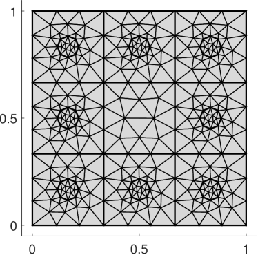
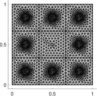
Figure 3: A coarser and a finer FEM-mesh for the diffusion example, both complying with the pixel partition and the measurement/excitation subdomains.

The FEM-approximated forward operator.

Given $l,r\in H^{\prime}$, we approximate the true measurement $\mathcal{F}_{l,r}(\sigma)=r(u_{\sigma}^{l})$ by

$$F_{l,r}(\sigma):=r(\tilde{u}_{\sigma}^{l}),$$

where $\tilde{u}_{\sigma}^{l}\in V$ is the FEM-approximation to the true solution $u_{\sigma}^{l}\in H$, i.e., the solution of (10).

Lemma 3

Let $l,r\in H^{\prime}$. Then

$$F_{l,r}(\sigma)=b_{\sigma}(\tilde{u}_{\sigma}^{l},\tilde{u}_{\sigma}^{r})\quad\text{ for all $\sigma\in\mathbb{R}^{n}_{+}$.}$$

Moreover, $F_{l,r}:\ \mathbb{R}^{n}_{+}\to\mathbb{R}$ is infinitely often differentiable and its first derivatives fulfill

$$\frac{\partial}{\partial\sigma_{i}}F_{l,r}(\sigma)=-b_{i}(\tilde{u}_{\sigma}^{l},\tilde{u}_{\sigma}^{r}),\quad i=1,\ldots,n.$$

Proof

This follows by applying corollary 1 to the Hilbert space $V$. $\Box$

From lemma 3, we obtain a simple FEM-based implementation of the forward operator and its derivative.

Corollary 2

With

$$\tilde{u}_{\sigma}^{l} =\sum_{j=1}^{N}\lambda^{l}_{j}\Lambda_{j},\qquad \lambda^{l} =(\lambda_{j}^{l})_{j=1}^{N}\in\mathbb{R}^{N},$$

$$\tilde{u}_{\sigma}^{r} =\sum_{j=1}^{N}\lambda^{r}_{j}\Lambda_{j},\qquad \lambda^{r} =(\lambda_{j}^{r})_{j=1}^{N}\in\mathbb{R}^{N},$$

we have that

$$F_{l,r}(\sigma)=(\lambda^{l})^{T}B_{\sigma}\lambda^{r}=(\lambda^{l})^{T}y^{r},\quad\text{ and }\quad\frac{\partial}{\partial\sigma_{i}}F_{l,r}(\sigma)=-(\lambda^{l})^{T}B_{i}\lambda^{r}.$$

Proof

This follows from lemma 3. $\Box$

We summarize the consequences of corollary 2 in algorithm 1. Using a FEM package that is capable of solving the considered PDE, and that allows access to the stiffness matrix and the load vector, one can simply implement the FEM-approximated forward operator and all its first derivatives by a few lines of extra code. This calculation merely requires solving two linear systems with the stiffness matrix (which is equivalent to two PDE solutions).

Algorithm 1 FEM-approximation of $F_{l,r}(\sigma)$ and $\frac{\partial}{\partial\sigma_{i}}F_{l,r}(\sigma)$, $i=1,\ldots,n$

  given $l,r\in H^{\prime}$, $\sigma\in\mathbb{R}^{n}_{+}$

  $\cdot$ use FEM package to calculate load vectors $y^{l}$ and $y^{r}$

  $\cdot$ use FEM package to calculate stiffness matrices $B_{\mathbbm{1}}$, and $B_{\mathbbm{1}+e_{i}}$ for all $i=1,\ldots,n$

  $\cdot$ set $B_{i}:=B_{\mathbbm{1}+e_{i}}-B_{\mathbbm{1}}$ for $i=1,\ldots,n$, and $B_{\sigma}:=B_{\mathbbm{1}}+\sum_{i=1}^{n}(\sigma_{i}-1)B_{i}$

  $\cdot$ solve $B_{\sigma}\lambda^{l}=y^{l}$ and $B_{\sigma}\lambda^{r}=y^{r}$ for $\lambda^{l}$ and $\lambda^{r}$

  return  $F_{l,r}(\sigma):=(\lambda^{l})^{T}y^{r}$ and $\frac{\partial}{\partial\sigma_{i}}F_{l,r}(\sigma):=-(\lambda^{l})^{T}B_{i}\lambda^{r}$, $i=1,\ldots,n$

Convergence of the FEM-approximated forward operator.

The following lemma shows that the FEM-approximated operator and its first derivatives agree with their true-solution counterparts as good as the FEM solution agrees with the true solution. Hence, by the Céa-Lemma (12), $F_{l,r}(\sigma)$ and $\frac{\partial}{\partial\sigma_{i}}F_{l,r}(\sigma)$ will be as good an approximation to $\mathcal{F}_{l,r}(\sigma)$ and $\frac{\partial}{\partial\sigma_{i}}\mathcal{F}_{l,r}(\sigma)$ as the true solutions can be approximated by elements of the finite-dimensional space $V$.

Lemma 4

For all $l,r\in H^{\prime}$ and $\sigma\in\mathbb{R}^{n}_{+}$, we have that:

$$\mathcal{F}_{l,r}(\sigma)-F_{l,r}(\sigma) =b_{\sigma}(u_{\sigma}^{l}-\tilde{u}_{\sigma}^{l},u_{\sigma}^{r}-\tilde{u}_{\sigma}^{r}),$$ (13)

$$\frac{\partial}{\partial\sigma_{i}}\mathcal{F}_{l,r}(\sigma)-\frac{\partial}{\partial\sigma_{i}}F_{l,r}(\sigma) =b_{i}(\tilde{u}_{\sigma}^{l},\tilde{u}_{\sigma}^{r}-u_{\sigma}^{r})+b_{i}(\tilde{u}_{\sigma}^{l}-u_{\sigma}^{l},u_{\sigma}^{r}).$$ (14)

Hence, by the Céa-Lemma (12),

$$0\leq\mathcal{F}_{l,r}(\sigma)-F_{l,r}(\sigma) \leq C_{\sigma}\hskip 0.86108pt\|u_{\sigma}^{l}-\tilde{u}_{\sigma}^{l}\|\hskip 0.86108pt\hskip 0.86108pt\|u_{\sigma}^{r}-\tilde{u}_{\sigma}^{r}\|\hskip 0.86108pt$$

$$\leq\frac{C_{\sigma}^{3}}{\beta_{\sigma}^{2}}\inf_{v\in V}\hskip 0.86108pt\|u_{\sigma}^{l}-v\|\hskip 0.86108pt\inf_{v\in V}\hskip 0.86108pt\|u_{\sigma}^{r}-v\|\hskip 0.86108pt,$$

and

$$\left|\frac{\partial}{\partial\sigma_{i}}\mathcal{F}_{l,r}(\sigma)-\frac{\partial}{\partial\sigma_{i}}F_{l,r}(\sigma)\right|$$

$$\leq C_{i}\hskip 0.86108pt\|\tilde{u}_{\sigma}^{l}\|\hskip 0.86108pt\hskip 0.86108pt\|\tilde{u}_{\sigma}^{r}-u_{\sigma}^{r}\|\hskip 0.86108pt+C_{i}\hskip 0.86108pt\|u_{\sigma}^{r}\|\hskip 0.86108pt\hskip 0.86108pt\|\tilde{u}_{\sigma}^{l}-u_{\sigma}^{l}\|\hskip 0.86108pt$$

$$\leq\frac{C_{i}C_{\sigma}}{\beta_{\sigma}}\left(\hskip 0.86108pt\|\tilde{u}_{\sigma}^{l}\|\hskip 0.86108pt\inf_{v\in V}\hskip 0.86108pt\|u_{\sigma}^{r}-v\|\hskip 0.86108pt+\hskip 0.86108pt\|u_{\sigma}^{r}\|\hskip 0.86108pt\inf_{v\in V}\hskip 0.86108pt\|u_{\sigma}^{l}-v\|\hskip 0.86108pt\right),$$

where $C_{i}>0$ is the continuity constant of $b_{i}(\cdot,\cdot)$.

Proof

Using

$$b_{\sigma}(\tilde{u}_{\sigma}^{l},\tilde{u}_{\sigma}^{r})=l(\tilde{u}_{\sigma}^{r})=b_{\sigma}(u_{\sigma}^{l},\tilde{u}_{\sigma}^{r}),\quad\text{ and }\quad b_{\sigma}(\tilde{u}_{\sigma}^{l},\tilde{u}_{\sigma}^{r})=r(\tilde{u}_{\sigma}^{l})=b_{\sigma}(\tilde{u}_{\sigma}^{l},u_{\sigma}^{r}),$$

we obtain (13) from

$$\mathcal{F}_{l,r}(\sigma)-F_{l,r}(\sigma) =b_{\sigma}(u_{\sigma}^{l},u_{\sigma}^{r})-b_{\sigma}(\tilde{u}_{\sigma}^{l},\tilde{u}_{\sigma}^{r})=b_{\sigma}(u_{\sigma}^{l},u_{\sigma}^{r}-\tilde{u}_{\sigma}^{r})$$

$$=b_{\sigma}(u_{\sigma}^{l},u_{\sigma}^{r}-\tilde{u}_{\sigma}^{r})-b_{\sigma}(\tilde{u}_{\sigma}^{l},u_{\sigma}^{r}-\tilde{u}_{\sigma}^{r})$$

$$=b_{\sigma}(u_{\sigma}^{l}-\tilde{u}_{\sigma}^{l},u_{\sigma}^{r}-\tilde{u}_{\sigma}^{r}).$$

Also,

$$\frac{\partial}{\partial\sigma_{i}}\mathcal{F}_{l,r}(\sigma)-\frac{\partial}{\partial\sigma_{i}}F_{l,r}(\sigma) =b_{i}(\tilde{u}_{\sigma}^{l},\tilde{u}_{\sigma}^{r})-b_{i}(u_{\sigma}^{l},u_{\sigma}^{r})$$

$$=b_{i}(\tilde{u}_{\sigma}^{l},\tilde{u}_{\sigma}^{r}-u_{\sigma}^{r})+b_{i}(\tilde{u}_{\sigma}^{l}-u_{\sigma}^{l},u_{\sigma}^{r}),$$

which shows (14). $\Box$

4.2 Convexity and monotonicity for symmetric measurements

As in subsection 3.2 we now consider the symmetric measurement case, where $l$ and $r$ are taken from the same subset of $H^{\prime}$ (and all combinations are used). Given a set of $m\in\mathbb{N}$ excitations/measurements $\{l_{1},\ldots,l_{m}\}\subset H^{\prime}$, we combine the measurements into a matrix-valued map $F:\ \mathbb{R}^{n}_{+}\to\mathbb{R}^{m\times m}$

$$F(\sigma)=(F_{j,k}(\sigma))_{j,k=1,\ldots,m}\in\mathbb{R}^{m\times m},\quad F_{j,k}(\sigma)=F_{l_{j},l_{k}}(\sigma)=l_{k}(u_{\sigma}^{l_{j}}).$$

The entries of $F(\sigma)$ and its first derivatives $\frac{\partial}{\partial\sigma_{i}}F(\sigma)$, $i=1,\ldots,n$ can be calculated as in algorithm 1. Let us stress that this approach is particularly efficient in this symmetric case as it requires only $m$ linear system solutions with the stiffness matrix (i.e., the equivalent of $m$ PDE solutions) for calculating all $m^{2}$ entries of $F(\sigma)\in\mathbb{R}^{m\times m}$ and all $nm^{2}$ entries of the $n$ matrices $\frac{\partial}{\partial\sigma_{i}}F(\sigma)\in\mathbb{R}^{m\times m}$.

As in subsection 3.2, the FEM-approximated forward operator is monotonically non-increasing and convex in the sense of the elementwise order ”$\geq$” on $\mathbb{R}^{n}$, and the Loewner order ”$\succeq$” on the set of symmetric $m\times m$-matrices.

Lemma 5

$F:\ \mathbb{R}^{n}_{+}\to\mathbb{R}^{m\times m}$ has the following properties:

1. $F$ is infinitely often differentiable.

2. For all $\sigma\in\mathbb{R}^{n}_{+}$, $F(\sigma)\in\mathbb{S}_{m}$ and $F(\sigma)\succeq 0$. $F(\sigma)$ is positive definite if $l_{1},\ldots,l_{m}\in H^{\prime}$ are linearly independent.

3. $F$ is monotonically non-increasing, i.e.

   $$F^{\prime}(\sigma)\tau\preceq 0\quad\text{ for all }\quad\sigma\in\mathbb{R}^{n}_{+},\ 0\leq\tau\in\mathbb{R}^{n},$$ (15)

4. $F$ is convex, i.e.

   $$F(\sigma)-F(\sigma^{(0)})\succeq F^{\prime}(\sigma^{(0)})(\sigma-\sigma^{(0)})\quad\text{ for all }\quad\sigma,\sigma^{(0)}\in\mathbb{R}^{n}_{+}.$$ (16)

5. $\mathcal{F}(\sigma)\succeq F(\sigma)$.

Proof

(a)–(d) follow from applying lemma 2 on the Hilbert space $V$. (e) was proven in lemma 4. $\Box$

5 Numerical examples and inverse problem challenges

In this section, we will show some numerical results for the stationary diffusion example from section 2.1 and demonstrate some major challenges that arise in solving the inverse coefficient problem of recovering $\hat{\sigma}\in\mathbb{R}^{n}$ from $\mathcal{F}(\hat{\sigma})\in\mathbb{R}^{m}$, or from a noisy version $Y^{\delta}\approx F(\hat{\sigma})$. The source codes for the following examples (and also for generating figure 1 and 2) are given in the appendix for the reader’s reference.

5.1 Non-uniqueness

Even for $m\geq n$, and a noise-free measurement $\hat{Y}=F(\hat{\sigma})\in\mathbb{R}^{m}$, it is not clear whether the measurements uniquely determine the unknown $\hat{\sigma}\in\mathbb{R}^{n}$. To demonstrate this on a simple one-dimensional example, let us consider the stationary diffusion example with $3\times 3$ pixels and circular excitation/measurement subdomains in each boundary pixel as in figure 1. We apply a source term in $D_{1}$ in the lower left pixel, and measure the resulting total concentration in $D_{8}$ in the top right pixel, so that $l=\chi_{1}\in H^{-1}(\Omega)$ and $r=\chi_{8}\in H^{-1}(\Omega)$, where we write $\chi_{j}:=\chi_{D_{j}}$ for the ease of notation. We choose $\sigma=1$ in all pixels except $\mathcal{P}_{i}$, and on $\mathcal{P}_{i}$ we vary the diffusivity in steps of $0.01$ up to $3$. Figure 4 shows $F_{l,r}(\sigma)$ for all $i=1,\ldots,9$, in the same order as the pixels, e.g., the lower left image shows $F_{l,r}(\sigma)$ for $\sigma=(\sigma_{1},1,\ldots,1)$ for varying $\sigma_{1}$.

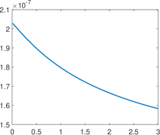
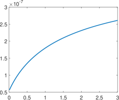
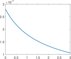
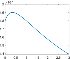
Figure 4: Single measurement in the top right pixel for a source term in the lower left pixel as a function of changing the diffusivity in each of the $3\times 3$ pixels.

Intuitively speaking, one can see that rising the diffusivity in the middle pixel increases the measurement since particles can easier diffuse through the middle pixel on their way from the lower left to the top right. Rising the diffusivity in the corner pixels decreases the measurement since particles can easier diffuse to the boundary that is set to zero by the homogeneous Dirichlet condition. In the middle top, left, bottom, and right pixel, rising the diffusivity first increases the measurement since particles can easier find their way from the lower left to the top right. But at some point, this effect is reverted since it also drives particles to the boundary.

This demonstrates that changing a coefficient can have an increasing or decreasing effect on the measurements, and the effect does not have to be monotonous for all parameter values. It also indicates that an exact one-dimensional measurement $\hat{Y}=F_{l,r}(\hat{\sigma})$ might uniquely determine one parameter in $\hat{\sigma}$ in some cases (here: the diffusivity in the middle and corner pixels), but non-uniqueness might occur in other cases (here: in the middle top, left, bottom, and right pixel).

Let us also stress the following point. A single non-symmetric measurement $F_{l,r}(\sigma)$ with $l\neq r$ might depend non-monotonously on $\sigma$ as demonstrated in figure 4. But, by lemma 5, for all $l,r\in H^{\prime}$, the symmetric measurements $F_{l,l}(\sigma)$, $F_{r,r}(\sigma)$, and also the matrix-valued measurement

$$\begin{pmatrix}F_{l,l}(\sigma)&F_{l,r}(\sigma)\\ F_{r,l}(\sigma)&F_{r,r}(\sigma)\end{pmatrix}\in\mathbb{R}^{2\times 2}$$

are monotonously non-increasing and convex functions of $\sigma$. Note that the monotonicity and convexity properties of the matrix-valued measurement hold with respect to the Loewner order even though the individual non-diagonal matrix elements might not have these properties.

5.2 Non-linearity and local minima

The inverse problem of recovering $\hat{\sigma}\in\mathbb{R}^{n}$ from $F(\hat{\sigma})\in\mathbb{R}^{m}$ could be considered as a non-linear root finding problem and (for $n=m$) approached with Newton’s method which is only known to converge locally. However, in practice one usually takes redundant measurements (i.e., $m>n$), and, due to measurement or modelling errors, one cannot expect exact data fit. Hence, a common approach to reconstruct $\hat{\sigma}\in\mathbb{R}^{n}$ from $Y^{\delta}\approx F(\hat{\sigma})\in\mathbb{R}^{m}$ is to minimize a residuum functional, e.g.,

$$R(\sigma):=\hskip 0.86108pt\|F(\sigma)-Y^{\delta}\|\hskip 0.86108pt^{2}\to\text{min!}$$

or a sum of a residuum functional together with a regularization term.

For our simple $3\times 3$-pixel example, the left image in figure 5 shows a contour plot of $R(\sigma)$ (in a normalized logarithmic scale) for a two-dimensional measurement function $F(\sigma):=\begin{pmatrix}F_{\chi_{1},\chi_{7}}(\sigma)&F_{\chi_{1},\chi_{8}}(\sigma)\end{pmatrix}\in\mathbb{R}^{2}$, exact data $Y^{\delta}=F(\hat{\sigma})$,

$$\hat{\sigma}=\begin{pmatrix}1&1&1&0.5&1&0.5&1&1&1\end{pmatrix}^{T}\quad\text{ and }\quad\sigma=\begin{pmatrix}1&1&1&\sigma_{4}&1&\sigma_{6}&1&1&1\end{pmatrix}^{T}.$$

$\sigma_{4}$ and $\sigma_{6}$ are varied in steps of $0.002$ up to $0.6$. Again, for this choice of unknowns and measurements, we numerically observe non-uniqueness. The results indicate that there is a second point $\tilde{\sigma}\neq\hat{\sigma}$ with $F(\tilde{\sigma})=F(\hat{\sigma})$.

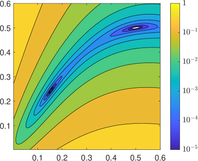
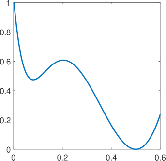
Figure 5: Residuum functional $R(\sigma)$ as a function of two parameters (left image), and as a function of one parameter (right image).

The right image in figure 5 shows a plot of $R(\sigma)$ (in a normalized non-logarithmic scale) for varying $\sigma_{4}$ while keeping $\sigma_{6}:=\sigma_{4}$, i.e. the diagonal of the left image in figure 5. It indicates that in this case, one parameter in $\hat{\sigma}$ can be uniquely reconstructed from the two-dimensional measurement $F(\hat{\sigma})$. But it also shows that the residuum functional $R(\sigma)$ possesses a local minimum in a wrong point. Since the curse of dimensionality makes it practically infeasible to numerically find the global minimizer of a non-linear functional in more than a few unknowns, this demonstrates that optimization-based approaches also suffer from only local convergence.

5.3 Stability, error estimates and ill-posedness

Even if $F(\hat{\sigma})$ uniquely determines $\hat{\sigma}$, and if this non-linear problem can be solved without running into a local minimum, the problem might be ill-posed in the sense that $\sigma$ does not depend stably on $F(\sigma)$. In that case, small errors in the measurements might lead to large errors in the reconstruction. The error amplification is often quantified by searching for a Lipschitz stability constant $L>0$ with

$$\hskip 0.86108pt\|\sigma_{1}-\sigma_{2}\|\hskip 0.86108pt\leq L\hskip 0.86108pt\|F(\sigma_{1})-F(\sigma_{2})\|\hskip 0.86108pt\quad\text{ for all }\sigma_{1},\sigma_{2}\in\mathbb{R}^{n}.$$

It should be stressed though, that such a stability estimate does not immediately yield an error estimate for noisy measurements $Y^{\delta}\approx F(\sigma)$, since $Y^{\delta}$ might not lie in the range of $F$.

To estimate the (relative) error amplification, we calculate the condition number of $F^{\prime}(\mathbbm{1})$ for our $3\times 3$ example, where $F:\ \mathbb{R}^{9}\to\mathbb{R}^{64}$ now depends on all $9$ pixel values, and the components of $F$ are given by $F_{l,r}$ with $l$ and $r$ running through all $8\times 8$-combinations of $\chi_{1},\ldots,\chi_{8}$, i.e., we use all combinations of circular subdomain for applying source terms and for measuring the solution. Note that, lemma 5 implies that roughly half of the measurements are redundant by symmetry, and that unlike in sections 3.2 and 4.2, we simply write the measurements as a long vector in order to have $F^{\prime}(\mathbbm{1})\in\mathbb{R}^{9,64}$ as a matrix.

We repeat the calculation of the condition number of $F^{\prime}(\mathbbm{1})$ for analogous settings with $n_{x}\times n_{x}$-pixels, and $(4n_{x}-4)\times(4n_{x}-4)$ measurements on circular subdomains in the boundary pixels, cf. the left image in figure 6 for the geometry of the $15\times 15$-pixel case. The right image in figure 6 shows the condition number as a function of the total number of pixels $n_{x}^{2}$ for $n_{x}\in\{2,3,\ldots,15\}$.

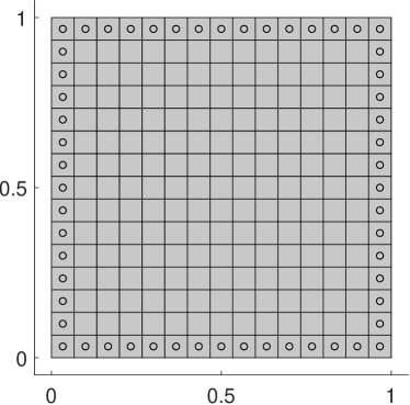
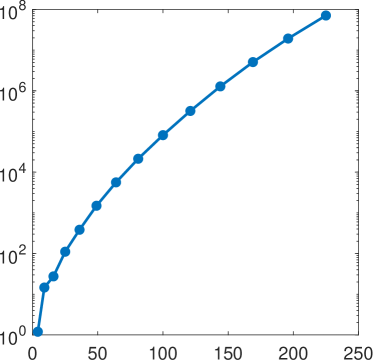
Figure 6: Condition number of $F^{\prime}(\mathbbm{1})$ as a function of the total number of pixels (right image) for pixel partitions ranging from $2\times 2$ to $15\times 15$ as sketched in left image.

Our results indicate that the instability of the considered inverse problem grows roughly exponentially with the number of unknowns which is in par with theoretical results on the similar elliptic inverse coefficient problem of EIT rondi2006remark .

5.4 Further reading

There is vast literature on theoretical and numerical inverse coefficient problems, their practical applications, and the regularization of ill-posed problems. Let us single out just a very few results as starting points for further reading that are closely connected to the challenges addressed in this section, and the author’s own research. Arguably the most prominent inverse elliptic coefficient problem is the so-called Calderón problem calderon1980inverse ; calderon2006inverse with applications in EIT, cf. adler2015electrical ; arridge2011methods for surveys on EIT and the related field of diffuse optical tomography. For theoretical uniqueness proofs in the infinite-dimensional setting of (intuitively speaking) infinitely many pixels and measurements we refer to uhlmann2009electrical ; harrach2009uniqueness ; kenig2014recent . A survey on solving parameter identification problems for PDEs with a focus on sparsity regularization can be found in jin2012sparsity . The interplay between instability, regularization and FEM discretization is studied in kaltenbacher2011adaptive . A result result on convexification approaches to obtain globally convergent reconstruction algorithms can be found in klibanov2019convexification . Learning-based approaches for inverse coefficient problems and parametrized PDEs are studied in arridge2019solving ; seo2019learning ; bhattacharya2020model .

Results on uniqueness and Lipschitz stability for finitely many unknowns from infinitely or finitely many measurements have been obtained in, e.g., alessandrini2005lipschitz ; alberti2019calderon ; harrach2019uniqueness . Let us stress that, for most problems, it is still an open question, how many (and which) measurements are required to uniquely determine an unknown PDE coefficient with a given resolution, how to explicitly quantify the error amplification, and how to obtain globally convergent reconstruction algorithms. For a relatively simple, but fully non-linear inverse problem of determining a Robin coefficient in an elliptic PDE, these question were recently answered in harrach2021uniqueness by exploiting the convexity and monotonicity structure of symmetric measurements from section 3.2 and 4.2.

Appendix A Appendix: Source code for COMSOL with MATLAB LiveLink

Listing 1–3 contain auxiliary functions to build and manipulate the FEM model. Figure 1–6 are created by listing 4–9.

Listing 1: Build_model.m

⬇

function model = Build_Model(nx)

%%%%%%%%%%%%%%%%%%%%%%%%%%%%%%%%%%%%%%%%%%%%%%%%%%%%%%%%%%%%%%%%%%

% Builds the model for the stationary diffusion example with

% nx\times nx pixels and excitations/measurements on circular

% subdomains located in the boundary pixels

%%%%%%%%%%%%%%%%%%%%%%%%%%%%%%%%%%%%%%%%%%%%%%%%%%%%%%%%%%%%%%%%%%

import com.comsol.model.*

import com.comsol.model.util.*

% Clear previously used models and create new one:

ModelUtil.clear; model = ModelUtil.create(’Model’);

n=nx*nx; model.param.set(’n’,n); % total number of pixels

m=4*nx-4; model.param.set(’m’,m); % total number of discs

% Create the outer domain Omega as unit square:

cp=model.component.create(’cp’);

setting=cp.geom.create(’setting’,2);

Omega=setting.create(’Omega’,’Square’); Omega.set(’size’,1);

Omega.set(’selresult’, true); Omega.set(’selresultshow’, ’bnd’);

% Create pixels, circular subdomains in boundary pixels,

% and variables to control diffusivity and soure terms

P_size=1/nx; D_radius=0.15*P_size;

allDnames=cell(1,m); iP=0; iD=0;

for j=1:nx

y=(j-1)*P_size;

for k=1:nx

x=(k-1)*P_size;

iP=iP+1; Pname=[’P’,num2str(iP)];

sigmaname=[’sigma’,num2str(iP)];

Pi=setting.create(Pname,’Square’);

Pi.set(’pos’, [x,y]); Pi.set(’size’,P_size);

Pi.set(’selresult’, true);

sigmai=cp.variable.create(sigmaname);

sigmai.selection.named([’setting_’,Pname,’_dom’]);

sigmai.set(’sigma’, 1);

if (j==1) || (j==nx) || (k==1) || (k==nx)

iD=iD+1; Dname=[’D’,num2str(iD)];

allDnames{iD}=Dname; lname=[’l’,num2str(iD)];

Di=setting.create(Dname, ’Circle’);

Di.set(’pos’, [x+0.5*P_size,y+0.5*P_size]);

Di.set(’r’,D_radius); Di.set(’selresult’, true);

li=cp.variable.create(lname);

li.selection.named([’setting_’,Dname,’_dom’]);

li.set(’g’, 1);

end

end

end

% Complement of union of circular subdomains in Omega:

notD=setting.create(’notD’, ’Difference’);

notD.selection(’input’).set({’Omega’});

notD.selection(’input2’).set(allDnames);

notD.set(’selresult’, true);

notD.set(’keep’, true);

l0=cp.variable.create(’l0’);

l0.selection.named(’setting_notD_dom’); l0.set(’g’, 0);

setting.run;

% Enter PDE and create FEM-mesh:

PDE=model.physics.create(’phys’,’CoefficientFormPDE’,’setting’);

PDE.feature(’cfeq1’).set(’c’,’sigma’);

PDE.feature(’cfeq1’).set(’f’, ’g’);

PDE.feature(’cfeq1’).set(’da’, {’0’});

bc=PDE.create(’boundary_condition’,’DirichletBoundary’,1);

bc.selection.named(’setting_Omega_bnd’);

FEM_mesh=cp.mesh.create(’FEM_mesh’);

FEM_mesh.run;

% Prepare solver and solution plot:

study_object=model.study.create(’study_object’);

study_object.feature.create(’stat’, ’Stationary’);

study_object.run;

plot_object=model.result.create(’plot_object’, ’PlotGroup2D’);

plot_object.set(’data’, ’dset1’);

surf_object=plot_object.create(’surf_object’, ’Surface’);

surf_object.set(’expr’, ’u’);

plot_object.run;

Listing 2: Set_Variables.m

⬇

function Set_Variables(model,sigma,l)

%%%%%%%%%%%%%%%%%%%%%%%%%%%%%%%%%%%%%%%%%%%%%%%%%%%%%%%%%%%%%%%%%%

% sets the model variables to given vectors sigma and l

%%%%%%%%%%%%%%%%%%%%%%%%%%%%%%%%%%%%%%%%%%%%%%%%%%%%%%%%%%%%%%%%%%

n=str2num(model.param.get(’n’));

m=str2num(model.param.get(’m’));

for i=1:n

sigmai=[’sigma’,num2str(i)];

model.component(’cp’).variable(sigmai).set(’sigma’, sigma(i));

end

for i=1:m

li=[’l’,num2str(i)];

model.component(’cp’).variable(li).set(’g’, l(i));

end

Listing 3: Build_Stiffness_and_Load.m

⬇

function [B_all_1,B,y]=Build_Stiffness_and_Load(model)

%%%%%%%%%%%%%%%%%%%%%%%%%%%%%%%%%%%%%%%%%%%%%%%%%%%%%%%%%%%%%%%%%%

% Calculates stiffness matrix B_all_1 % (with sigma=1 everywhere),

% B{i}: pixel stiffness matrix of i-th pixel, and

% y: matrix with columnwise load vector y_j

% for excitation on j-th circle

%%%%%%%%%%%%%%%%%%%%%%%%%%%%%%%%%%%%%%%%%%%%%%%%%%%%%%%%%%%%%%%%%%

n=str2double(model.param.get(’n’));

m=str2double(model.param.get(’m’));

l=zeros(1,m); sigma=ones(1,n); Set_Variables(model,sigma,l);

FEM_struct=mphmatrix(model,’sol1’,’out’,’Kc’);

B_all_1=FEM_struct.Kc;

B=cell(1,n);

y=zeros(size(B_all_1,1),m);

for j=1:n

sigma=ones(1,n); sigma(j)=2;

if j<=m

l=zeros(1,m); l(j)=1;

Set_Variables(model,sigma,l);

FEM_struct=mphmatrix(model,’sol1’,’out’,{’Kc’,’Lc’});

y(:,j)=FEM_struct.Lc;

else

Set_Variables(model,sigma,l);

FEM_struct=mphmatrix(model,’sol1’,’out’,{’Kc’});

end

B{j}=FEM_struct.Kc-B_all_1;

end

Listing 4: Plot_Figure_Setting.m

⬇

function Plot_Figure_Setting

%%%%%%%%%%%%%%%%%%%%%%%%%%%%%%%%%%%%%%%%%%%%%%%%%%%%%%%%%%%%%%%%%%

% Creates the two images in figure 1

%%%%%%%%%%%%%%%%%%%%%%%%%%%%%%%%%%%%%%%%%%%%%%%%%%%%%%%%%%%%%%%%%%

model = Build_Model(3);

m=str2double(model.param.get(’m’));

n=str2double(model.param.get(’n’));

f=figure;

mphviewselection(model,’setting_notD_dom’,…

’edgecolorselected’,[0,0,0],’facecolorselected’,’w’,…

’facecolor’,’gray’);

title(”);

for j=1:m

Dname=[’D’,num2str(j)]; Dlabel=[’$D_’,num2str(j),’$’];

Dcenter=str2num(…

model.geom(’setting’).feature(Dname).getString(’pos’));

text(Dcenter(1),Dcenter(2),Dlabel,’HorizontalAlignment’,…

’center’,’FontSize’,14,’Interpreter’,’latex’);

% also remove Dj for the next plot:

model.geom(’setting’).feature.remove(Dname);

end

set(gca,’XTick’,[0,0.5,1],’YTick’,[0,0.5,1],’FontSize’,14);

axis([-0.05,1.05,-0.05,1.05])

exportgraphics(f,’fig_pixel_partition_with_circs.eps’,…

’ContentType’,’vector’);

% remove complement of circles to only plot pixel partion

model.geom(’setting’).feature.remove(’notD’);

% Plot the pixel partition:

f=figure; mphgeom(model); title(”);

for i=1:n

Pname=[’P’,num2str(i)];

Plabel=[’$\mathcal P_’,num2str(i),’$’];

Ppos=str2num(…

model.geom(’setting’).feature(Pname).getString(’pos’));

Psize=str2num(…

model.geom(’setting’).feature(Pname).getString(’size’));

text(Ppos(1)+Psize/2,Ppos(2)+Psize/2,Plabel,…

’HorizontalAlignment’,’center’,’FontSize’,14,…

’Interpreter’,’latex’);

end

set(gca,’XTick’,[0,0.5,1],’YTick’,[0,0.5,1],’FontSize’,14);

axis([-0.05,1.05,-0.05,1.05])

exportgraphics(f,’fig_pixel_partition.pdf’,’ContentType’,’vector’);

Listing 5: Plot_Figure_Excitations.m

⬇

function Plot_Figure_Excitations

%%%%%%%%%%%%%%%%%%%%%%%%%%%%%%%%%%%%%%%%%%%%%%%%%%%%%%%%%%%%%%%%%%

% Creates the two images in figure 2

%%%%%%%%%%%%%%%%%%%%%%%%%%%%%%%%%%%%%%%%%%%%%%%%%%%%%%%%%%%%%%%%%%

model = Build_Model(3);

sigma=[1,1,1,1,1,1,1,1,1];

l=[0,1,0,1,1,0,1,0];

Set_Variables(model,sigma,l);

model.study(’study_object’).run;

model.result(’plot_object’).run;

f=figure; mphplot(model); title(”); xlabel(”); ylabel(”);

set(gca,’XTick’,[0,0.5,1],’YTick’,[0,0.5,1],’FontSize’,14);

axis([-0.05,1.05,-0.05,1.05])

exportgraphics(f,’fig_excitations1.pdf’,’ContentType’,’vector’);

l=[1,0,1,0,0,1,0,1];

Set_Variables(model,sigma,l);

model.study(’study_object’).run;

model.result(’plot_object’).run;

f=figure; mphplot(model); title(”); xlabel(”); ylabel(”);

set(gca,’XTick’,[0,0.5,1],’YTick’,[0,0.5,1],’FontSize’,14);

axis([-0.05,1.05,-0.05,1.05])

exportgraphics(f,’fig_excitations2.pdf’,’ContentType’,’vector’);

Listing 6: Plot_Figure_CompliantMesh.m

⬇

function Plot_Figure_CompliantMesh

%%%%%%%%%%%%%%%%%%%%%%%%%%%%%%%%%%%%%%%%%%%%%%%%%%%%%%%%%%%%%%%%%%

% Creates the two images in figure 3

%%%%%%%%%%%%%%%%%%%%%%%%%%%%%%%%%%%%%%%%%%%%%%%%%%%%%%%%%%%%%%%%%%

model = Build_Model(3);

% Coarser mesh:

model.component(’cp’).mesh(’FEM_mesh’).feature…

(’size’).set(’hauto’,8);

model.component(’cp’).mesh(’FEM_mesh’).run;

f=figure; mphmesh(model); title(”); xlabel(”); ylabel(”);

set(gca,’XTick’,[0,0.5,1],’YTick’,[0,0.5,1],’FontSize’,14);

axis([-0.05,1.05,-0.05,1.05])

exportgraphics(f,’fig_compliant_mesh.pdf’,’ContentType’,’vector’);

% Finer mesh:

model.component(’cp’).mesh(’FEM_mesh’).feature…

(’size’).set(’hauto’,3);

model.component(’cp’).mesh(’FEM_mesh’).run;

f=figure; mphmesh(model); title(”); xlabel(”); ylabel(”);

set(gca,’XTick’,[0,0.5,1],’YTick’,[0,0.5,1],’FontSize’,14);

axis([-0.05,1.05,-0.05,1.05])

exportgraphics(f,’fig_compliant_mesh_fine.pdf’,…

’ContentType’,’vector’);

Listing 7: Plot_Figure_Non_uniqueness.m

⬇

function Plot_Figure_Non_uniqueness

%%%%%%%%%%%%%%%%%%%%%%%%%%%%%%%%%%%%%%%%%%%%%%%%%%%%%%%%%%%%%%%%%%

% Creates the nine images in figure 4

%%%%%%%%%%%%%%%%%%%%%%%%%%%%%%%%%%%%%%%%%%%%%%%%%%%%%%%%%%%%%%%%%%

model = Build_Model(3);

[B_all_1,B,y]=Build_Stiffness_and_Load(model);

y_l=y(:,1); y_r=y(:,end);

sigma=linspace(0.01,3,300);

F=zeros(9,length(sigma));

parfor j=1:length(sigma)

for i=1:9

B_sigma=B_all_1+(sigma(j)-1)*B{i};

lambda_l=B_sigma\y_l;

F(i,j)=y_r’*lambda_l;

end

end

for j=1:9

figname=[’fig_non_uniqueness’,num2str(j),’.pdf’];

f=figure; plot(sigma,F(j,:),’LineWidth’,2);

set(gca,’FontSize’,16);

exportgraphics(f,figname,’ContentType’,’vector’);

end

Listing 8: Plot_Figure_Residuals.m

⬇

function Plot_Figure_Residuals

%%%%%%%%%%%%%%%%%%%%%%%%%%%%%%%%%%%%%%%%%%%%%%%%%%%%%%%%%%%%%%%%%%

% Creates the two images in figure 5

%%%%%%%%%%%%%%%%%%%%%%%%%%%%%%%%%%%%%%%%%%%%%%%%%%%%%%%%%%%%%%%%%%

model = Build_Model(3);

[B_all_1,B,y]=Build_Stiffness_and_Load(model);

y_l=y(:,1); y_r1=y(:,end); y_r2=y(:,end-1); B_4=B{4}; B_6=B{6};

B_sigmahat=B_all_1-0.5*B_4-0.5*B_6;

lambdahat_l=B_sigmahat\y_l;

Fhat_1=y_r1’*lambdahat_l;

Fhat_2=y_r2’*lambdahat_l;

n=300;

sigma4_range=linspace(0,0.6,n+1);

sigma4_range=sigma4_range(2:end);

sigma6_range=linspace(0,0.6,n+1);

sigma6_range=sigma6_range(2:end);

[S4range,S6range]=meshgrid(sigma4_range,sigma6_range);

F_1=zeros(n,n); F_2=F_1;

parfor j=1:n

for k=1:n

sigma4=S4range(j,k); sigma6=S6range(j,k);

B_sigma=B_all_1+(sigma4-1)*B_4+(sigma6-1)*B_6;

lambda_l=B_sigma\y_l;

F_1(j,k)=y_r1’*lambda_l;

F_2(j,k)=y_r2’*lambda_l;

end

end

R=(F_1-Fhat_1).^2+(F_2-Fhat_2).^2; R=R/max(max(R));

f=figure; contourf(S4range,S6range,log10(R),[-5:0.5:0]);

axis square;

set(gca,’XTick’,0:0.1:0.6,’YTick’,0:0.1:0.6,’FontSize’,14);

c_handle=colorbar;

set(c_handle,’TickLabels’,{’$10^{-5}$’,’$10^{-4}$’,’$10^{-3}$’,…

’$10^{-2}$’,’$10^{-1}$’,’$1$’},…

’TickLabelInterpreter’,’latex’,’FontSize’,14);

exportgraphics(f,’fig_residuals_2D.pdf’,’ContentType’,’vector’);

f=figure;

plot(diag(S4range),diag(R)/max(diag(R)),’LineWidth’,2);

set(gca,’FontSize’,14); axis square;

exportgraphics(f,’fig_residuals_1D.pdf’,’ContentType’,’vector’);

Listing 9: Plot_Figure_Stability.m

⬇

function Plot_Figure_Stability

%%%%%%%%%%%%%%%%%%%%%%%%%%%%%%%%%%%%%%%%%%%%%%%%%%%%%%%%%%%%%%%%%%

% Creates the two images in figure 6

%%%%%%%%%%%%%%%%%%%%%%%%%%%%%%%%%%%%%%%%%%%%%%%%%%%%%%%%%%%%%%%%%%

nx=2:15;

condnumbers=zeros(size(nx));

for j=1:length(nx)

model = Build_Model(nx(j));

[B_all_1,B,y]=Build_Stiffness_and_Load(model);

lambda=B_all_1\y;

n=str2double(model.param.get(’n’));

m=str2double(model.param.get(’m’));

dF=zeros(m*m,n);

for i=1:n

d_iF=-lambda’*B{i}*lambda;

dF(:,i)=d_iF(:);

end

condnumbers(j)=cond(dF);

end

f=figure;

semilogy(nx.^2,condnumbers,’.-’,’LineWidth’,2,’MarkerSize’,20);

axis square; set(gca,’FontSize’,14);

exportgraphics(f,’fig_stability.pdf’,’ContentType’,’vector’);

% also plot setting with finest pixel partition

f=figure; mphgeom(model); title(”);

set(gca,’XTick’,[0,0.5,1],’YTick’,[0,0.5,1],’FontSize’,14);

axis([-0.05,1.05,-0.05,1.05])

exportgraphics(f,’fig_setting_stability.pdf’,…

’ContentType’,’vector’);

References

- [1] A. Adler, R. Gaburro, and W. Lionheart. Electrical impedance tomography. In Handbook of Mathematical Methods in Imaging, pages 701–762. Springer, 2015.
- [2] G. S. Alberti and M. Santacesaria. Calderón’s inverse problem with a finite number of measurements. In Forum of Mathematics, Sigma, volume 7. Cambridge University Press, 2019.
- [3] G. Alessandrini and S. Vessella. Lipschitz stability for the inverse conductivity problem. Advances in Applied Mathematics, 35(2):207–241, 2005.
- [4] S. Arridge, P. Maass, O. Öktem, and C.-B. Schönlieb. Solving inverse problems using data-driven models. Acta Numerica, 28:1–174, 2019.
- [5] S. R. Arridge. Methods in diffuse optical imaging. Philosophical Transactions of the Royal Society A: Mathematical, Physical and Engineering Sciences, 369(1955):4558–4576, 2011.
- [6] K. Bhattacharya, B. Hosseini, N. B. Kovachki, and A. M. Stuart. Model reduction and neural networks for parametric pdes. arXiv preprint arXiv:2005.03180, 2020.
- [7] A. P. Calderón. On an inverse boundary value problem. In W. H. Meyer and M. A. Raupp, editors, Seminar on Numerical Analysis and its Application to Continuum Physics, pages 65–73. Brasil. Math. Soc., Rio de Janeiro, 1980.
- [8] A. P. Calderón. On an inverse boundary value problem. Comput. Appl. Math., 25(2–3):133–138, 2006.
- [9] M. Hanke. A regularizing Levenberg-Marquardt scheme, with applications to inverse groundwater filtration problems. Inverse problems, 13(1):79, 1997.
- [10] B. Harrach. On uniqueness in diffuse optical tomography. Inverse Problems, 25:055010 (14pp), 2009.
- [11] B. Harrach. Uniqueness and Lipschitz stability in electrical impedance tomography with finitely many electrodes. Inverse Problems, 35(2):024005, 2019.
- [12] B. Harrach. Uniqueness, stability and global convergence for a discrete inverse elliptic Robin transmission problem. Numerische Mathematik, 147:29–70, 2021.
- [13] B. Jin and P. Maass. Sparsity regularization for parameter identification problems. Inverse Problems, 28(12):123001, 2012.
- [14] B. Kaltenbacher, A. Kirchner, and B. Vexler. Adaptive discretizations for the choice of a tikhonov regularization parameter in nonlinear inverse problems. Inverse Problems, 27(12):125008, 2011.
- [15] C. Kenig and M. Salo. Recent progress in the Calderón problem with partial data. Contemp. Math, 615:193–222, 2014.
- [16] M. V. Klibanov, J. Li, and W. Zhang. Convexification of electrical impedance tomography with restricted Dirichlet-to-Neumann map data. Inverse Problems, 2019.
- [17] L. Rondi. A remark on a paper by Alessandrini and Vessella. Advances in Applied Mathematics, 36(1):67–69, 2006.
- [18] J. K. Seo, K. C. Kim, A. Jargal, K. Lee, and B. Harrach. A learning-based method for solving ill-posed nonlinear inverse problems: a simulation study of lung EIT. SIAM Journal on Imaging Sciences, 12(3):1275–1295, 2019.
- [19] E. Somersalo, M. Cheney, and D. Isaacson. Existence and uniqueness for electrode models for electric current computed tomography. SIAM J. Appl. Math., 52(4):1023–1040, 1992.
- [20] G. Uhlmann. Electrical impedance tomography and Calderón’s problem. Inverse problems, 25(12):123011, 2009.