Numerical approximation of the spectrum of self-adjoint continuously invertible operators

Abstract

This paper deals with the generalized spectrum of continuously invertible linear operators defined on infinite dimensional Hilbert spaces. More precisely, we consider two bounded, coercive, and self-adjoint operators ${\mathcal{A},B}:V\mapsto V^{\#}$, where $V^{\#}$ denotes the dual of $V$, and investigate the conditions under which the whole spectrum of ${\mathcal{B}}^{-1}{\mathcal{A}}:V\mapsto V$ can be approximated to an arbitrary accuracy by the eigenvalues of the finite dimensional discretization ${\mathcal{B}}_{n}^{-1}{\mathcal{A}}_{n}$. Since ${\mathcal{B}}^{-1}{\mathcal{A}}$ is continuously invertible, such an investigation cannot use the concept of uniform (normwise) convergence, and it relies instead on the pointwise (strong) convergence of ${\mathcal{B}}_{n}^{-1}{\mathcal{A}}_{n}$ to ${\mathcal{B}}^{-1}{\mathcal{A}}$.

The paper is motivated by operator preconditioning which is employed in the numerical solution of boundary value problems. In this context, ${\mathcal{A}},{\mathcal{B}}:H_{0}^{1}(\Omega)\mapsto H^{-1}(\Omega)$ are the standard integral/functional representations of the differential operators $-\nabla\cdot(k(x)\nabla u)$ and $-\nabla\cdot(g(x)\nabla u)$, respectively, and $k(x)$ and $g(x)$ are scalar coefficient functions. The investigated question differs from the eigenvalue problem studied in the numerical PDE literature which is based on the approximation of the eigenvalues within the framework of compact operators.

This work follows the path started by the two recent papers published in [SIAM J. Numer. Anal., 57 (2019), pp. 1369-1394 and 58 (2020), pp. 2193-2211] and addresses one of the open questions formulated at the end of the second paper.

Keywords: Second order PDEs, bounded non-compact operators, generalized spectrum, numerical approximation, preconditioning.

1 Introduction.

Extending the path of research started in [14, 7, 8], this paper will consider the differential operators $-\nabla\cdot(k(x)\nabla u)$ and $-\nabla\cdot(g(x)\nabla u)$ on the open and bounded Lipschitz domain $\Omega\subset\mathbb{R}^{2}$, where the scalar functions $g(x)$ and $k(x)$ are uniformly positive and continuous throughout the closure $\overline{\Omega}$. The associated operator representations ${\mathcal{A}},\,{\mathcal{B}}:H_{0}^{1}(\Omega)\mapsto H^{-1}(\Omega)$, are given by

$$\langle\mathcal{A}u,v\rangle=\int_{\Omega}k(x)\nabla u\cdot\nabla v,\quad u,v\in H_{0}^{1}(\Omega),$$ (1)

$$\langle\mathcal{B}u,v\rangle=\int_{\Omega}g(x)\nabla u\cdot\nabla v,\quad u,v\in H_{0}^{1}(\Omega).$$ (2)

In the first part of this paper we characterize the spectrum of the preconditioned operator

$${\mathcal{B}}^{-1}{\mathcal{A}}:H_{0}^{1}(\Omega)\to H_{0}^{1}(\Omega),$$ (3)

defined as the complement of the resolvent set, i.e.,

$$\mathrm{sp}(\mathcal{B}^{-1}\mathcal{A}):=\left\{\lambda\in\mathbb{C};\,\lambda\mathcal{I}-\mathcal{B}^{-1}\mathcal{A}\mbox{ does not have a bounded inverse}\right\}.$$ (4)

More specifically, we prove that

$$\mathrm{sp}(\mathcal{L}^{-1}\mathcal{A})=\left[\inf_{x\in\overline{\Omega}}\ \frac{k(x)}{g(x)},\,\sup_{x\in\overline{\Omega}}\ \frac{k(x)}{g(x)}\right].$$

Consider a sequence of finite dimensional subspaces of $H_{0}^{1}(\Omega)$ defined via the nodal polynomial basis functions $\phi_{1},\ldots,\phi_{n}$ with the local supports

$${\mathcal{T}}_{j}=\mbox{supp}(\phi_{j}),\quad j=1,\ldots,n.$$ (5)

The standard Galerkin finite element discretization of the operators ${\mathcal{A}}$ and ${\mathcal{B}}$ gives the matrix representations of the discretised operators $\mathcal{A}_{n}$ and $\mathcal{B}_{n}$ in terms of the basis $\phi_{1},\ldots,\phi_{n}$,

$$[{\mathbf{A}}_{n}]_{ij} =\int_{\Omega}k(x)\nabla\phi_{j}\cdot\nabla\phi_{i},\,\quad i,j=1,\ldots,n.$$ (6)

$$[{\mathbf{B}}_{n}]_{ij} =\int_{\Omega}g(x)\nabla\phi_{j}\cdot\nabla\phi_{i},\,\quad i,j=1,\ldots,n.$$ (7)

Part one of this paper also contains an investigation of the approximation of the whole spectrum of ${\mathcal{B}}^{-1}{\mathcal{A}}$ by the eigenvalues of the preconditioned matrices ${\mathbf{B}}_{n}^{-1}{\mathbf{A}}_{n}$ as $n\rightarrow\infty$.

In the second part, i.e., in section 4, we generalize the results obtained for (1) and (2). More precisely, the spectrum issue is explored in terms of an abstract setting where ${\mathcal{A}},{\mathcal{B}}:V\mapsto V^{\#}$ only are assumed to be bounded, coercive, and self-adjoint linear operators. Here, $V^{\#}$ denotes the dual of $V$ consisting of all linear bounded functionals from the infinite dimensional Hilbert space $V$ to $\mathbb{R}$. We present a condition under which the whole spectrum of ${\mathcal{B}}^{-1}{\mathcal{A}}:V\mapsto V$, defined as the complement of the resolvent set, is approximated as $n\rightarrow\infty$ to an arbitrary accuracy by the eigenvalues of the finite dimensional discretizations ${\mathcal{B}}_{n}^{-1}{\mathcal{A}}_{n}$. More precisely, we will concentrate on Galerkin discretizations using a sequence $\{V_{n}\}$ of subspaces $V_{n}\subset V$ satisfying the approximation property

$$\lim_{n\rightarrow\infty}\inf_{v\in V_{n}}\|w-v\|=0\quad\mbox{for all}\;w\in V\,.$$ (8)

Since ${\mathcal{B}}^{-1}{\mathcal{A}}$ is continuously invertible and $V$ is of infinite dimension, such an investigation cannot be based on the uniform (normwise) convergence, and it relies instead upon the pointwise (strong) convergence of ${\mathcal{B}}_{n}^{-1}{\mathcal{A}}_{n}$ to ${\mathcal{B}}^{-1}{\mathcal{A}}$.

2 Preconditioning by Laplacian ($g(x)=1$).

Considering the case $g(x)=1$, i.e., the preconditioner equals the operator representation of the Laplacian ${\mathcal{B}}={\mathcal{L}}$, the paper [8] determines the spectrum of the preconditioned operator ${\mathcal{L}}^{-1}{\mathcal{A}}$ in the following way (for brevity we use a bit stronger assumptions than in [8] and consider a uniformly positive scalar coefficient function $k(x)$):

Theorem 2.1 (cf. [8], Theorem 1.1).

Consider an open and bounded Lipschitz domain $\Omega\subset\mathbb{R}^{2}$. Assume that the scalar function $k(x)$ is uniformly positive and continuous throughout the closure $\overline{\Omega}$. Then the spectrum of the operator ${\mathcal{L}}^{-1}{\mathcal{A}}$ equals the interval

$$\mathrm{sp}(\mathcal{L}^{-1}\mathcal{A})=\left[\inf_{x\in\overline{\Omega}}\ k(x),\,\sup_{x\in\overline{\Omega}}\ k(x)\right].$$ (9)

In other words, for a uniformly positive continuous function $k(x)$, the spectrum of ${\mathcal{L}}^{-1}{\mathcal{A}}$ equals the range $k(\overline{\Omega})$.

Eigenvalues of the discretized operator $\mathcal{L}_{n}^{-1}\mathcal{A}_{n}$, that is represented by the matrix ${\mathbf{L}}_{n}^{-1}{\mathbf{A}}_{n}$, can be approximated using the following theorem from [7]. (Here we again use assumptions conforming to the setting in the current paper.)

Theorem 2.2 (cf. [7], Theorem 3.1).

Let $0<\lambda_{1}\leq\lambda_{2}\leq\ldots\leq\lambda_{n}$ be the eigenvalues of ${\mathbf{L}}_{n}^{-1}{\mathbf{A}}_{n}$, where ${\mathbf{A}}_{n}$ and ${\mathbf{L}}_{n}$ are defined in (6) and (7), respectively. Let $k(x)$ be uniformly positive and continuous throughout the closure $\overline{\Omega}$. Then there exist a (possibly non-unique) permutation $\pi$ such that the eigenvalues $\lambda_{\pi(j)}$ of the matrix ${\mathbf{L}}_{n}^{-1}{\mathbf{A}}_{n}$ satisfy

$$\lambda_{\pi(j)}\in\left[\inf_{x\in{\mathcal{T}}_{j}}k(x),\sup_{x\in{\mathcal{T}}_{j}}k(x)\right],\quad j=1,\ldots,n,$$ (10)

where ${\mathcal{T}}_{j}$ is defined in (5).

Consequently, there is a one-to-one mapping (possibly non-unique) between the eigenvalues of ${\mathbf{L}}_{n}^{-1}{\mathbf{A}}_{n}$ and the ranges of $k(x)$ over the supports of the individual basis functions. With an appropriate grid refinement of the discretization, the size of the intervals containing the individual eigenvalues of ${\mathbf{L}}_{n}^{-1}{\mathbf{A}}_{n}$ converge linearly to zero.

The paper [8] formulates a dual open question about the distribution of the eigenvalues of the discretized operators within the interval (9). Assuming in addition that $k(x)\in{\mathcal{C}}^{2}(\overline{\Omega})$, we will now show that theorems 2.1 and 2.2 yield that any point in the spectrum of the infinite dimensional operator ${\mathcal{L}}^{-1}{\mathcal{A}}$ is approximated, as $n\rightarrow\infty$, to an arbitrary accuracy by the eigenvalues (10) of the matrices ${\mathbf{L}}_{n}^{-1}{\mathbf{A}}_{n}$. The individual points in the infinite dimensional spectrum can, however, be approximated with different speed that is at least linear and uniformly bounded from zero.

Consider an arbitrary point $\mu$ in the spectrum of the operator ${\mathcal{L}}^{-1}{\mathcal{A}}$. It should be noted that $\mu$ may not be an eigenvalue, and that our investigation differs from the eigenvalue problem studied in the numerical PDE literature which is based on approximations of the eigenvalues within the framework of infinite dimensional compact solution operators.

Using theorem 2.1, $\mu$ is the image under $k(x)$ of some point $y\in\overline{\Omega}$, i.e., $\mu=k(y)$. We first consider the case $y\in{\Omega}$. The case $y\in{\partial\Omega}$ will be resolved later by a simple limiting argument. Let $\varepsilon>0$ be an arbitrarily small positive constant, and let

$$\delta=\frac{\varepsilon}{2\sup_{x\in\Omega}\|\nabla k(x)\|},$$

provided that $\sup_{x\in\Omega}\|\nabla k(x)\|>0$. (The case $\sup_{x\in\Omega}\|\nabla k(x)\|=0$ is uninteresting because then ${\mathcal{A}}=c{\mathcal{L}}$ for some constant $c$.) Consider further a Galerkin discretization such that the support of at least one of the nodal basis functions that contains the point $y$ is itself contained in the disc with center $y$ and radius $\delta$. Denote this support ${\mathcal{T}}_{j}$ and the associated eigenvalue of the discretized operator given by theorem 2.2 as $\lambda_{\pi(j)}$. Using Corollary 3.2 in [7] (with $y=\hat{x}_{j}$)

$$|\lambda_{\pi(j)}-k(y)| \leq\sup_{x\in{\mathcal{T}}_{j}}\|k(x)-k(y)\|$$

$$\leq\delta\,\|\nabla k(y)\|+\frac{1}{2}\delta^{2}\sup_{x\in{\mathcal{T}}_{j}}\|D^{2}k(x)\|,$$ (11)

where $D^{2}k(x)$ denotes the second order derivative of the function $k(x)$. For $\varepsilon$ sufficiently small we thus get, after a simple manipulation,

$$|\lambda_{\pi(j)}-\mu|\leq\varepsilon.$$ (12)

If $\mu=k(y)$ and $y\in\partial\Omega$, the same conclusion can be obtained using the previous derivation and the continuity of $k(x)$ throughout $\overline{\Omega}.$ Summing up, this proves the following theorem:

Theorem 2.3 (Approximation of the spectrum by matrix eigenvalues).

Let $k(x)$ be twice continuously differentiable and uniformly positive throughout the closure $\overline{\Omega}$. Let the maximal diameter of the local supports of the basis functions used in the Galerkin discretization (5)-(7) vanishes as $n\rightarrow\infty$. Then any point in the spectrum of the operator ${\mathcal{L}}^{-1}{\mathcal{A}}$ is for $n\rightarrow\infty$ approximated to an arbitrary accuracy by the eigenvalues of the matrices ${\mathbf{L}}_{n}^{-1}{\mathbf{A}}_{n}$ representing the discretized preconditioned operators.

The linear part of the upper bound (11) for the approximation error is for the individual spectral points $\mu$ proportional to the size of the gradient $\|\nabla k(y)\|$, where $k(y)=\mu$. Since the size of this gradient is uniformly bounded from above throughout $\overline{\Omega}$, the speed of convergence towards the individual spectral points, as the h-refinement proceeds, is uniformly bounded from zero throughout the whole spectrum of ${\mathcal{L}}^{-1}{\mathcal{A}}$. It can however differ for different spectral points.

3 Generalization to (piecewise) continuous and uniformly positive $g(x)$.

The purpose of this section is to generalize the results presented above to preconditioners in the form (2). We first present the theorems and a corollary, and thereafter their proofs are discussed.

The content of the present section is motivated by the desire to increase our knowledge about second order differential operators and preconditioning issues. In particular, to obtain a better understanding of the benefits of applying piecewise constant preconditioners.

Theorem 3.1 (Spectrum of the infinite dimensional preconditioned operator).

Consider an open and bounded Lipschitz domain $\Omega\subset\mathbb{R}^{2}$. Assume that the scalar functions $g(x)$ and $k(x)$ are uniformly positive and continuous throughout the closure $\overline{\Omega}$. Then the spectrum of the operator ${\mathcal{B}}^{-1}{\mathcal{A}}$, defined in (4), equals

$$\mathrm{sp}(\mathcal{B}^{-1}\mathcal{A})=\left[\inf_{x\in\overline{\Omega}}\ \frac{k(x)}{g(x)},\,\sup_{x\in\overline{\Omega}}\ \frac{k(x)}{g(x)}\right].$$ (13)

The next theorem deals with the localization of the eigenvalues of the preconditioned matrix arising from the discretization. It does not consider the approximation of the spectrum of the infinite dimensional operator ${\mathcal{B}}^{-1}{\mathcal{A}}$. Analogously to [7], we can therefore relax the assumptions about the continuity of the coefficient functions $k(x)$ and $g(x)$.

Theorem 3.2 (Eigenvalues of the preconditioned matrix).

Let $0<\lambda_{1}\leq\lambda_{2}\leq\ldots\leq\lambda_{n}$ be the eigenvalues of ${\mathbf{B}}_{n}^{-1}{\mathbf{A}}_{n}$, where ${\mathbf{A}}_{n}$ and ${\mathbf{B}}_{n}$ are defined in (6) and (7), respectively. Let $g(x)$ and $k(x)$ be bounded, uniformly positive and piecewise continuous functions. Then there exists a (possibly non-unique) permutation $\pi$ such that the eigenvalues of the matrix ${\mathbf{B}}_{n}^{-1}{\mathbf{A}}_{n}$ satisfy

$$\lambda_{\pi(j)}\in\left[{\inf_{x\in{\mathcal{T}}_{j}}}\frac{k(x)}{g(x)},{\sup_{x\in{\mathcal{T}}_{j}}}\frac{k(x)}{g(x)}\right],\quad j=1,\ldots,n,$$ (14)

where ${\mathcal{T}}_{j}$ is defined in (5).

Corollary 3.3 (Pairing the eigenvalues and the nodal values).

Using the notation and the assumptions of Theorem 3.2, consider any point ${\hat{x}_{j}}\in{{\mathcal{T}}_{j}}$. Then the associated eigenvalue $\lambda_{\pi(j)}$ of the matrix ${\mathbf{B}}^{-1}{\mathbf{A}}$ satisfies

$$|\lambda_{\pi(j)}-r({\hat{x}_{j}})|\leq{\sup_{x\in{\mathcal{T}}_{j}}}|r(x)-r({\hat{x}_{j}})|,\quad{j=1,\ldots,n,}$$ (15)

where

$$r(x)\equiv\frac{k(x)}{g(x)}.$$

If, in addition, $k(x)$ and $g(x)\in{\mathcal{C}}^{2}({{\mathcal{T}}_{j}})$, then

$$|\lambda_{\pi(j)}-r({\hat{x}_{j}})| \leq{\sup_{x\in{\mathcal{T}}_{j}}}|r(x)-r({\hat{x}_{j}})|$$

$$\leq\hat{h}\|\nabla r({\hat{x}_{j}})\|+\tfrac{1}{2}\hat{h}^{2}{\sup_{x\in{\mathcal{T}}_{j}}}\|D^{2}r(x)\|,\quad{j=1,\ldots,n,}$$ (16)

where $\hat{h}={\mathrm{diam}({\mathcal{T}}_{j})}$ and $D^{2}r(x)$ denotes the second order derivative of $r(x)$. In particular, (15) and (16) hold for any discretization mesh node ${\hat{x}_{j}}\in{{\mathcal{T}}_{j}}$.

While the proofs of Theorem 3.1 and Theorem 3.2 are presented below, Corollary 3.3 follows immediately by applying [7, Corollary 3.2] to the ratio function $r(x)$.

Proof of Theorem 3.1.

Recall the definition (2) of the operator ${\mathcal{B}}$, and let us introduce the following notation for the inner product and norm induced by ${\mathcal{B}}$,

$$(u,v)_{{\mathcal{B}}} =\langle\mathcal{B}u,v\rangle,\quad u,v\in H_{0}^{1}(\Omega),$$

$$\|u\|_{{\mathcal{B}}}^{2} =(u,u)_{{\mathcal{B}}},\quad u\in H_{0}^{1}(\Omega).$$

1. The proof of the fact that

   $$\mathrm{sp}(\mathcal{B}^{-1}\mathcal{A})\subset\left[\inf_{x\in\overline{\Omega}}\ \frac{k(x)}{g(x)},\,\sup_{x\in\overline{\Omega}}\ \frac{k(x)}{g(x)}\right]$$

   is analogous to the proof in [8, Section 3], employing the inner product induced by ${\mathcal{B}}$ instead of that induced by the Laplacian ${\mathcal{L}}$. More precisely, using the self-adjointness of the operator ${\mathcal{B}}^{-1}{\mathcal{A}}$ with respect to the inner product $(\cdot,\cdot)_{{\mathcal{B}}}$, the spectrum of ${\mathcal{B}}^{-1}{\mathcal{A}}$ is real and it is contained in the interval

   $$\mathrm{sp}(\mathcal{B}^{-1}\mathcal{A}) \subset\left[\inf_{u\in H_{0}^{1}(\Omega)}\frac{({\mathcal{B}}^{-1}{\mathcal{A}}u,u)_{{\mathcal{B}}}}{(u,u)_{{\mathcal{B}}}},\ \sup_{u\in H_{0}^{1}(\Omega)}\frac{({\mathcal{B}}^{-1}{\mathcal{A}}u,u)_{{\mathcal{B}}}}{(u,u)_{{\mathcal{B}}}}\right]$$

   $$=\left[\inf_{u\in H_{0}^{1}(\Omega)}\frac{\langle{\mathcal{A}}u,u\rangle}{\langle{\mathcal{B}}u,u\rangle},\ \sup_{u\in H_{0}^{1}(\Omega)}\frac{\langle{\mathcal{A}}u,u\rangle}{\langle{\mathcal{B}}u,u\rangle}\right].$$ (17)

   Moreover, the endpoints of this interval are contained in the spectrum. It remains to bound

   $$\frac{\langle{\mathcal{A}}u,u\rangle}{\langle{\mathcal{B}}u,u\rangle}$$ (18)

   in terms of the values of the scalar functions $g(x)$ and $k(x)$. Let $\|\cdot\|$ denote the standard Euclidean norm. Then,

   $$\sup_{u\in H_{0}^{1}(\Omega)}\frac{\langle{\mathcal{A}}u,u\rangle}{\langle{\mathcal{B}}u,u\rangle} =\sup_{u\in H_{0}^{1}(\Omega)}\frac{\int_{\Omega}k(x)\|\nabla u\|^{2}}{\int_{\Omega}g(x)\|\nabla u\|^{2}}=\sup_{u\in H_{0}^{1}(\Omega)}\frac{\int_{\Omega}\frac{k(x)}{g(x)}g(x)\|\nabla u\|^{2}}{\int_{\Omega}g(x)\|\nabla u\|^{2}}$$

   $$\leq\sup_{x\in\Omega}\frac{k(x)}{g(x)},$$ (19)

   where we have used the assumption that $k(x)$ and $g(x)$ are uniformly positive and continuous on $\overline{\Omega}$. Similarly,

   $$\inf_{u\in H_{0}^{1}(\Omega)}\frac{\langle{\mathcal{A}}u,u\rangle}{\langle{\mathcal{L}}u,u\rangle} \geq\inf_{x\in\Omega}\frac{k(x)}{g(x)}.$$ (20)

2. The proof of the converse inclusion

   $$\left[\inf_{x\in\overline{\Omega}}\ \frac{k(x)}{g(x)},\,\sup_{x\in\overline{\Omega}}\ \frac{k(x)}{g(x)}\right]\subset\mathrm{sp}(\mathcal{B}^{-1}\mathcal{A})$$

   is similar to the proof of [14, Theorem 3.1].

   • For an arbitrary $x_{0}\in\Omega$, consider $\lambda_{0}=k(x_{0})/g(x_{0})$.

   • Let $\{v_{r}\}_{r\in\mathbb{R}_{+}}$ be a set of functions satisfying

     $${\rm supp}(v_{r})\subset x_{0}+U_{r},$$ (21)

     $$\|v_{r}\|_{{\mathcal{B}}}=1,$$ (22)

     where $U_{r}=\{z\in\mathbb{R}^{2}|\;\|z\|\leq r\}$.

   • Next, let

     $$u_{r}=(\lambda_{0}{\mathcal{I}}-{\mathcal{B}}^{-1}{\mathcal{A}})v_{r},$$ (23)

     and observe that

     $${\mathcal{B}}u_{r}=(\lambda_{0}{\mathcal{B}}-{\mathcal{A}})v_{r}.$$

     Consequently (see (2)),

     $$\|u_{r}\|_{{\mathcal{B}}}^{2} =\langle(\lambda_{0}{\mathcal{B}}-{\mathcal{A}})v_{r},u_{r}\rangle$$

     $$=\int_{x_{0}+U_{r}}\left(g(x)\lambda_{0}-k(x)\right)\nabla v_{r}\cdot\nabla u_{r}$$

     $$\leq\sup_{x\in x_{0}+U_{r}}\left|g(x)\frac{k(x_{0})}{g(x_{0})}-k(x)\right|\,g_{\mathrm{min}}^{-1}\,|(v_{r},u_{r})_{{\mathcal{B}}}|$$

     $$\leq\sup_{x\in x_{0}+U_{r}}\left|g(x)\frac{k(x_{0})}{g(x_{0})}-k(x)\right|\,g_{\mathrm{min}}^{-1}\,\|v_{r}\|_{{\mathcal{B}}}\|u_{r}\|_{{\mathcal{B}}},$$

     where

     $${\color[rgb]{0,0,0}g_{\mathrm{min}}=\min_{x\in x_{0}+U_{r}}g(x).}$$

     Employing (22),

     $$\|u_{r}\|_{{\mathcal{B}}}\leq\sup_{x\in x_{0}+U_{r}}\left|g(x)\frac{k(x_{0})}{g(x_{0})}-k(x)\right|\,g_{\mathrm{min}}^{-1},$$

     and from the continuity of $g(x)$ and $k(x)$ we conclude that

     $$\lim_{r\to 0}\|u_{r}\|_{{\mathcal{B}}}=0.$$ (24)

   • Assume that $\lambda_{0}\notin\mathrm{sp}(\mathcal{B}^{-1}\mathcal{A})$. Then $\lambda_{0}{\mathcal{I}}-{\mathcal{B}}^{-1}{\mathcal{A}}$ has a bounded inverse, and (23) and (24) imply that

     $$\|v_{r}\|_{{\mathcal{B}}}\leq\|(\lambda_{0}{\mathcal{I}}-{\mathcal{B}}^{-1}{\mathcal{A}})^{-1}\|_{{\mathcal{B}}}\,\|u_{r}\|_{{\mathcal{B}}}\longrightarrow 0$$

     as $r\rightarrow 0$, which contradicts (22). We conclude that

     $$\lambda_{0}=\frac{k(x_{0})}{g(x_{0})}\in\mathrm{sp}(\mathcal{B}^{-1}\mathcal{A}).$$

   • Since $x_{0}\in\Omega$ was arbitrary in this argument, and $g$ and $k$ are continuous and uniformly positive on $\overline{\Omega}$, it follows that

     $$\left(\inf_{x\in\overline{\Omega}}\ \frac{k(x)}{g(x)},\,\sup_{x\in\overline{\Omega}}\ \frac{k(x)}{g(x)}\right)\subset\mathrm{sp}(\mathcal{B}^{-1}\mathcal{A}).$$ (25)

     As mentioned above, according to the general result for self-adjoint operators, the endpoints of the interval in (17) are contained in the spectrum of ${\mathcal{B}}^{-1}{\mathcal{A}}$. Combining this with (19) and (20) yield that also the endpoints of the interval (25) belong to $\mathrm{sp}(\mathcal{B}^{-1}\mathcal{A})$.

Proof Theorem 3.2.

The proof of Theorem 3.2 is analogous to the proof of Theorem 3.1 in[7]. As was explained in detail in [9, Section 3.2], due to the use of the Hall’s theorem for bipartite graphs (see, e.g., [2, Theorem 5.2]), it is sufficient to prove the statement formulated in the following lemma (cf. [7, Lemma 3.3]).

Lemma 3.4.

Assume that $k(x)$ and $g(x)$ are uniformly positive, bounded and piecewise continuous functions, and let the matrix ${\mathbf{B}}_{n}^{-1}{\mathbf{A}}_{n}$ be given by (6) and (7). Let, moreover, ${\mathcal{J}}\subset\{1,\ldots,n\}$ and let ${\mathcal{T}}_{\mathcal{J}}:=\bigcup_{j\in{\mathcal{J}}}{\mathcal{T}}_{j}$ be the union of the supports of the basis functions $\phi_{j}$, $j\in{\mathcal{J}}$. Then there are at least $|{\mathcal{J}}|$ eigenvalues of the matrix ${\mathbf{B}}_{n}^{-1}{\mathbf{A}}_{n}$ located in the interval

$$\left[{\inf_{x\in{\mathcal{T}}_{\mathcal{J}}}}\frac{k(x)}{g(x)},{\sup_{x\in{\mathcal{T}}_{\mathcal{J}}}}\frac{k(x)}{g(x)}\right].$$ (26)

Proof.

Following the proof of Lemma 3.3 in [7], consider, for any set of indices ${\mathcal{J}}\subset\{1,\ldots,n\}$, the (local) perturbation $\tilde{k}_{\mathcal{J}}(x)$ of the coefficient function $k(x)$,

$$\tilde{k}_{\mathcal{J}}(x) =\begin{cases}K\cdot g(x)\qquad\mbox{for}\quad x\in{\mathcal{T}}_{{\mathcal{J}}},\\ k(x)\quad\mbox{elsewhere},\end{cases}$$ (27)

where $K$ is a positive scalar. Analogously to (6), the matrix $\tilde{{\mathbf{A}}}_{{\mathcal{J}},n}$ obtained by the discretization of the associated perturbed operator $\tilde{{\mathcal{A}}}_{{\mathcal{J}}}$ is given by

$$[\tilde{{\mathbf{A}}}_{{\mathcal{J}},n}]_{lj} =\left\langle\tilde{{\mathcal{A}}}_{{\mathcal{J}},h}\phi_{j},\phi_{l}\right\rangle=\int_{\Omega}\tilde{k}_{{\mathcal{J}}}(x)\nabla\phi_{j}\cdot\nabla\phi_{l}\,.$$

The simple observation

$$\tilde{{\mathbf{A}}}_{{\mathcal{J}},n}{\mathbf{e}}_{j}=K\,{\mathbf{B}}_{n}{\mathbf{e}}_{j},\quad j\in{{\mathcal{J}}},$$

shows that $K$ is an eigenvalue of the matrix ${\mathbf{B}}_{n}^{-1}\tilde{{\mathbf{A}}}_{{\mathcal{J}},n}$ with multiplicity of at least $|{\mathcal{J}}|$.

By similarity transformations, the spectrum of ${\mathbf{B}}_{n}^{-1}{\mathbf{A}}_{n}$ equals the spectrum of ${\mathbf{B}}_{n}^{-1/2}{\mathbf{A}}_{n}{\mathbf{B}}_{n}^{-1/2}$, and the spectrum of ${\mathbf{B}}_{n}^{-1}\tilde{{\mathbf{A}}}_{{\mathcal{J}},n}$ is equal to the spectrum of ${\mathbf{B}}_{n}^{-1/2}\tilde{{\mathbf{A}}}_{{\mathcal{J}},n}{\mathbf{B}}_{n}^{-1/2}$. Using the standard perturbation result for symmetric matrices (see, e.g., [15, Corollary 4.9, p. 203]), there are at least $|{\mathcal{J}}|$ eigenvalues of ${\mathbf{B}}_{n}^{-1}{\mathbf{A}}_{n}$ in the interval

$$[K+\theta_{min},K+\theta_{max}]\subset[K-\Theta,K+\Theta],$$ (28)

where $\Theta=\max\{|\theta_{min}|,|\theta_{max}|\}$ and $\theta_{min}$ and $\theta_{max}$ denote the smallest and largest eigenvalues, respectively, of the perturbation matrix ${\mathbf{B}}_{n}^{-1}({\mathbf{A}}_{n}-\tilde{{\mathbf{A}}}_{{\mathcal{J}},n})$.

The Rayleigh quotient for an eigenvalue-eigenvector pair $(\theta,{\mathbf{q}})$ of the perturbation matrix, with the associated eigenfunction $q=\sum_{j=1}^{N}\nu_{j}\phi_{j},\,{\mathbf{q}}^{T}=[\nu_{1},\ldots,\nu_{N}]$, satisfies

$$\theta =\frac{{\mathbf{q}}^{T}({\mathbf{A}}_{n}-\tilde{{\mathbf{A}}}_{{\mathcal{J}},n}){\mathbf{q}}}{{\mathbf{q}}^{T}{\mathbf{B}}_{n}{\mathbf{q}}}=\frac{\langle({\mathcal{A}}-\tilde{{\mathcal{A}}}_{{\mathcal{J}}})q,q\rangle}{\langle{\mathcal{B}}q,q\rangle}$$

$$=\frac{\int_{\Omega}(k(x)-\tilde{k}_{{\mathcal{J}}}(x))\nabla q\cdot\nabla q\,dx}{\int_{\Omega}g(x)\|\nabla q\|^{2}\,dx}=\frac{\int_{{\mathcal{T}}_{{\mathcal{J}}}}(k(x)-Kg(x))\|\nabla q\|^{2}\,dx}{\int_{\Omega}g(x)\|\nabla q\|^{2}\,dx}$$

$$=\frac{\int_{{\mathcal{T}}_{{\mathcal{J}}}}\left(\frac{k(x)}{g(x)}-K\right)g(x)\|\nabla q\|^{2}\,dx}{\int_{\Omega}g(x)\|\nabla q\|^{2}\,dx},$$

where we used the fact that $\tilde{k}_{{\mathcal{J}}}(x)=k(x)$ for $x\in\Omega\setminus{\mathcal{T}}_{{\mathcal{J}}}$; see (27). Using the uniform positivity of $g(x)$,

$$|\theta|\leq{\sup_{x\in{\mathcal{T}}_{{\mathcal{J}}}}}\left|\frac{k(x)}{g(x)}-K\right|.$$ (29)

Substituting (29) into (28) yields the existence of at least $|{\mathcal{J}}|$ eigenvalues of ${\mathbf{B}}_{{\color[rgb]{0,0,0}n}}^{-1}{\mathbf{A}}_{{\color[rgb]{0,0,0}n}}$ in the interval

$$\left[\,K-{\sup_{x\in{\mathcal{T}}_{{\mathcal{J}}}}}\left|\frac{k(x)}{g(x)}-K\right|,\,K+{\sup_{x\in{\mathcal{T}}_{{\mathcal{J}}}}}\left|\frac{k(x)}{g(x)}-K\right|\,\right].$$ (30)

Setting $K=\tfrac{1}{2}\left(\inf_{x\in{\mathcal{T}}_{{\mathcal{J}}}}\frac{k(x)}{g(x)}+\sup_{x\in{\mathcal{T}}_{{\mathcal{J}}}}\frac{k(x)}{g(x)}\right)$ finishes the proof. ∎

4 Abstract setting.

This section investigates numerical approximations of the spectrum of preconditioned linear operators within an abstract Hilbert space setting; see, e.g., [13, 10]. Let $V$ be an infinite dimensional real Hilbert space with the inner product

$$(\cdot,\cdot):V\times V\mapsto\mathbb{R}.$$ (31)

Throughout this text, $V^{\#}$ denotes the dual of $V$ consisting of all linear bounded functionals from $V$ to $\mathbb{R}$, with the associated duality pairing

$$\langle\cdot,\cdot\rangle:V^{\#}\times V\mapsto\mathbb{R},$$

and the Riesz map

$$\langle\cdot,\cdot\rangle=:(\tau\cdot,\cdot),\quad\tau:V^{\#}\mapsto V.$$

Consider two bounded and coercive linear operators ${\mathcal{A}},{\mathcal{B}}:V\mapsto V^{\#}$ that are self-adjoint with respect to the duality pairing. We will investigate whether all the points in the spectrum of the preconditioned operator ${\mathcal{B}}^{-1}{\mathcal{A}}:V\mapsto V$ are approximated to an arbitrary accuracy by the eigenvalues of the finite dimensional operators in a sequence $\{{\mathcal{B}}_{n}^{-1}{\mathcal{A}}_{n}\}$ determined via the Galerkin discretization.

For the problems considered in sections 2 and 3, we obtained concrete expressions for the approximations of the spectrum of ${\mathcal{B}}^{-1}{\mathcal{A}}$ in terms of the coefficient functions $g(x)$ and $k(x)$. Such detailed information is, of course, not obtainable for the present abstract problem setting. We must be content with analyzing whether, or in what sense, the set of eigenvalues of the discretized mapping converges toward the spectrum of the corresponding infinite dimensional operator.

Since ${\mathcal{B}}^{-1}{\mathcal{A}}$ is self-adjoint with respect to the inner product

$$(\cdot,\cdot)_{{\mathcal{B}}}:=\langle{\mathcal{B}}\,\cdot,\cdot\rangle:V\times V\mapsto\mathbb{R},$$ (32)

it is convenient to use this inner product instead of (31) whenever appropriate. The associated norm $\|\cdot\|_{{\mathcal{B}}}$ is equivalent to the norm $\|\cdot\|$ defined by the inner product (31), and the Riesz map $\tau_{{\mathcal{B}}}$ representing the operator preconditioning is determined by

$$\langle\cdot,\cdot\rangle=:(\tau_{{\mathcal{B}}}\,\cdot,\cdot)_{{\mathcal{B}}}=\langle{\mathcal{B}}\,\tau_{{\mathcal{B}}}\,\cdot,\cdot\rangle,\quad\mbox{i.e.,}\;\tau_{{\mathcal{B}}}={\mathcal{B}}^{-1}.$$

The investigated preconditioned operator ${\mathcal{B}}^{-1}{\mathcal{A}}$ is continuously invertible on the Hilbert space $V$ of infinite dimension. Therefore its finite dimensional approximations can not converge to it in norm (uniformly). We will instead use Theorem 4.1 (below) that assumes the pointwise (strong) convergence. Its statement reformulates a theorem presented in [11, chapter VIII, § 1.2, Theorem 1.14, p. 431], which is reproduced also in [3, section 5.4, Theorem 5.12, pp. 239-240]. The second monograph also provides several references to related results of J. Descloux and collaborators published earlier; see, in particular, [6]. In terms of the spectral representation of self-adjoint operators, a bit stronger statements were proved in the context of the problem of moments in [16, section III.3, Theorem IX, p. 61] and, more generally, in [11, chapter VIII, § 1.2, Theorem 1.15, p. 432]. The formulations in [11] and [3] require a careful study of parts of the books. We will therefore, for the sake of convenience, include a proof of the following theorem in the Appendix.

Theorem 4.1 (Approximation of the spectrum of self-adjoint operators).

Let ${\mathcal{Z}}$ be a linear self-adjoint operator on a Hilbert space $V$ and let $\{{\mathcal{Z}}_{n}\}$ be a sequence of linear self-adjoint operators on $V$ converging to ${\mathcal{Z}}$ pointwise (strongly). Then, for any point $\lambda\in\mathrm{sp}({\mathcal{Z}})$ in the spectrum of ${\mathcal{Z}}$, and for any of its neighbourhoods, there exists ${\mathcal{Z}}_{j}$ such that the intersection of its spectrum $\mathrm{sp}({\mathcal{Z}}_{j})$ with this neighbourhood is nonempty.

Using this theorem and the Hilbert space $V$ equipped with the inner product (32), it remains, within our setting, to prove that the self-adjoint operators ${\mathcal{Z}}_{n}$, which arise from ${\mathcal{B}}_{n}^{-1}{\mathcal{A}}_{n}$ by extending it to the whole space $V$, converge pointwise to the original self-adjoint operator

$${\mathcal{Z}}:={\mathcal{B}}^{-1}{\mathcal{A}}.$$

The discretization will be based on a sequence of subspaces $\{V_{n}\},\,V_{n}\subset V,$ satisfying the approximation property (8)

$$\lim_{n\rightarrow\infty}\inf_{v\in V_{n}}\|w-v\|=0\quad\mbox{for all}\;w\in V,$$ (33)

see, e.g., [1, relation (8)]. Note that (33) typically yields that Galerkin discretizations of boundary value problems are consistent; see also [13, chapter 9, relation (9.8)].

Consider a basis $\Phi_{n}=(\phi_{1}^{(n)},\dots,\phi_{n}^{(n)})$ of the $n$-dimensional subspace $V_{n}\subset V$. Then the Galerkin discretizations ${\mathcal{A}}_{n}$ and ${\mathcal{B}}_{n}$ of the operators ${\mathcal{A}}$ and ${\mathcal{B}}$ are determined by (see [10, section 4.1] and [13, chapter 6]),

$$\langle\mathcal{A}_{n}w,v\rangle:=\langle\mathcal{A}w,v\rangle\quad\mbox{and}\quad\langle\mathcal{B}_{n}w,v\rangle:=\langle\mathcal{B}w,v\rangle,\quad\mbox{for all}\;w,v\in V_{n}.$$ (34)

Their matrix representations are given by

$$\mathbf{A}_{n}=\left(\langle\mathcal{A}\phi_{j}^{(n)},\phi_{i}^{(n)}\rangle\right)_{i,j=1,\dots,n},$$ (35)

and

$$\mathbf{B}_{n}=\left(\langle\mathcal{B}\phi_{j}^{(n)},\phi_{i}^{(n)}\rangle\right)_{i,j=1,\dots,n}.$$ (36)

The spectrum of the discretized operator ${\mathcal{B}}_{n}^{-1}{\mathcal{A}}_{n}:V_{n}\mapsto V_{n}$ is given by the eigenvalues of its matrix representation $\mathbf{B}_{n}^{-1}\mathbf{A}_{n}$. The operator ${\mathcal{B}}_{n}^{-1}{\mathcal{A}}_{n}$ is self-adjoint with respect to the inner product (32), and the matrix $\mathbf{B}_{n}^{-1}\mathbf{A}_{n}$ is self-adjoint with respect to the algebraic inner product $(\mathbf{x},\mathbf{y})_{\mathbf{B}_{n}}:=\mathbf{y}^{*}\mathbf{B}_{n}\mathbf{x}$.

Using the orthogonal projection

$$\Pi_{{\mathcal{B}}}^{n}:V\mapsto V_{n},$$

where the orthogonality is determined by the inner product (32), ${\mathcal{B}}_{n}^{-1}{\mathcal{A}}_{n}$ is extended to the whole space $V$,

$${\mathcal{Z}}_{n}:={\mathcal{B}}_{n}^{-1}{\mathcal{A}}_{n}\,\Pi_{{\mathcal{B}}}^{n}:V\mapsto V_{n}\subset V.$$ (37)

We need to show that ${\mathcal{Z}}_{n}$ is self-adjoint with respect to the inner product (32). Using, for any $u,w\in V$, the associated orthogonal decompositions $u=\Pi_{{\mathcal{B}}}^{n}u+u^{\perp}$ and $w=\Pi_{{\mathcal{B}}}^{n}w+w^{\perp}$, we can write

$$\langle{\mathcal{B}}{\mathcal{Z}}_{n}u,w\rangle =\langle{\mathcal{B}}{\mathcal{B}}_{n}^{-1}{\mathcal{A}}_{n}\,\Pi_{{\mathcal{B}}}^{n}u,w\rangle=\langle{\mathcal{B}}{\mathcal{B}}_{n}^{-1}{\mathcal{A}}_{n}\,\Pi_{{\mathcal{B}}}^{n}u,\Pi_{{\mathcal{B}}}^{n}w\rangle+\langle{\mathcal{B}}{\mathcal{B}}_{n}^{-1}{\mathcal{A}}_{n}\,\Pi_{{\mathcal{B}}}^{n}u,w^{\perp}\rangle$$

$$=\langle{\mathcal{B}}_{n}{\mathcal{B}}_{n}^{-1}{\mathcal{A}}_{n}\,\Pi_{{\mathcal{B}}}^{n}u,\Pi_{{\mathcal{B}}}^{n}w\rangle=\langle{\mathcal{A}}_{n}\,\Pi_{{\mathcal{B}}}^{n}u,\Pi_{{\mathcal{B}}}^{n}w\rangle=\langle{\mathcal{A}}_{n}\,\Pi_{{\mathcal{B}}}^{n}w,\Pi_{{\mathcal{B}}}^{n}u\rangle$$

$$=\langle{\mathcal{B}}_{n}{\mathcal{B}}_{n}^{-1}{\mathcal{A}}_{n}\,\Pi_{{\mathcal{B}}}^{n}w,\Pi_{{\mathcal{B}}}^{n}u\rangle=\langle{\mathcal{B}}{\mathcal{B}}_{n}^{-1}{\mathcal{A}}_{n}\,\Pi_{{\mathcal{B}}}^{n}w,\Pi_{{\mathcal{B}}}^{n}u\rangle$$

$$=\langle{\mathcal{B}}{\mathcal{B}}_{n}^{-1}{\mathcal{A}}_{n}\,\Pi_{{\mathcal{B}}}^{n}w,\Pi_{{\mathcal{B}}}^{n}u\rangle+\langle{\mathcal{B}}{\mathcal{B}}_{n}^{-1}{\mathcal{A}}_{n}\,\Pi_{{\mathcal{B}}}^{n}w,u^{\perp}\rangle$$

$$=\langle{\mathcal{B}}{\mathcal{B}}_{n}^{-1}{\mathcal{A}}_{n}\,\Pi_{{\mathcal{B}}}^{n}w,u\rangle=\langle{\mathcal{B}}{\mathcal{Z}}_{n}w,u\rangle,$$

which gives the self-adjointness.

Summarizing, the sequence of subspaces $\{V_{n}\}$ determines a sequence of self-adjoint operators $\{{\mathcal{Z}}_{n}\}$ defined on the whole space $V$. The dimension of the ranges of these operators is finite, but increases as $n$ increases. It remains to prove that $\{{\mathcal{Z}}_{n}\}$ converges pointwise to ${\mathcal{Z}}$.

Theorem 4.2 (Pointwise convergence).

Let ${\mathcal{Z}}={\mathcal{B}}^{-1}{\mathcal{A}}$ be a linear self-adjoint operator on a Hilbert space $V$, where ${\mathcal{A}},{\mathcal{B}}:V\mapsto V^{\#}$ are bounded and coercive linear operators that are self-adjoint with respect to the duality pairing, and let $\{{\mathcal{Z}}_{n}\}$ be the sequence of linear self-adjoint operators defined in (37). Assume that the sequence of subspaces $\{V_{n}\}$ satisfy the approximation property (33). Then the sequence $\{{\mathcal{Z}}_{n}\}$ converges pointwise (strongly) to ${\mathcal{Z}}$, i.e., for all $w\in V$

$$\lim_{n\rightarrow\infty}\|{\mathcal{Z}}w-{\mathcal{Z}}_{n}w\|=0.$$

Proof.

Let $w\in V$ be an arbitrary fixed element and define

$$f:={\mathcal{Z}}w.$$

Consider a finite dimensional subspace $V_{n}\subset V$ and the Galerkin discretization of the equation ${\mathcal{Z}}w=f$, using the innerproduct $(\cdot,\cdot)_{{\mathcal{B}}}$: Find $w_{n}\in V_{n}$ such that

$$({\mathcal{Z}}w_{n},v)_{{\mathcal{B}}}=(f,v)_{{\mathcal{B}}}\quad\mbox{for all }v\in V_{n}.$$

This gives, for all $v\in V_{n}$,

$$0 =(f-{\mathcal{Z}}w_{n},v)_{{\mathcal{B}}}=(f_{n}-{\mathcal{Z}}w_{n},v)_{{\mathcal{B}}}+(f-f_{n},v)_{{\mathcal{B}}}$$

$$=(f_{n}-\widehat{{\mathcal{Z}}_{n}}w_{n},v)_{{\mathcal{B}}},$$ (38)

where we used the definition $f_{n}=\Pi_{{\mathcal{B}}}^{n}f$ for the discretized right hand side, i.e.,

$$(f_{n}-f,v)_{{\mathcal{B}}}=0\quad\mbox{for all}\;v\in V_{n},$$

giving

$$\|f-f_{n}\|_{{\mathcal{B}}}=\inf_{g\in V_{n}}\|f-g\|_{{\mathcal{B}}}.$$

The equivalence of the norms induced by the innerproducts (31) and (32) and the approximation property (33) then assure that

$$\lim_{n\rightarrow\infty}\|f-f_{n}\|=0\,.$$ (39)

The discretized operator $\widehat{{\mathcal{Z}}_{n}}$ is determined by

$$(\widehat{{\mathcal{Z}}_{n}}u,v)_{{\mathcal{B}}}:=({\mathcal{Z}}u,v)_{{\mathcal{B}}}\quad\mbox{for all}\;u,v\in V_{n},$$

and it is easy to verify that $\widehat{{\mathcal{Z}}_{n}}={\mathcal{B}}_{n}^{-1}{\mathcal{A}}_{n}$. Indeed, for all $u,v\in V_{n}$,

$$(\widehat{{\mathcal{Z}}_{n}}u,v)_{{\mathcal{B}}} =({\mathcal{B}}^{-1}{\mathcal{A}}u,v)_{{\mathcal{B}}}$$

$$=\langle{\mathcal{A}}u,v\rangle$$

$$=\langle{\mathcal{A}}_{n}u,v\rangle$$

$$=\langle{\mathcal{B}}_{n}{\mathcal{B}}_{n}^{-1}{\mathcal{A}}_{n}u,v\rangle$$

$$=\langle{\mathcal{B}}{\mathcal{B}}_{n}^{-1}{\mathcal{A}}_{n}u,v\rangle$$

$$=({\mathcal{B}}_{n}^{-1}{\mathcal{A}}_{n}u,v)_{{\mathcal{B}}}.$$

The previous considerations remain valid when replacing $\widehat{{\mathcal{Z}}_{n}}$ by its extension ${\mathcal{Z}}_{n}$ to the whole space $V$ given in (37) because

$$({\mathcal{Z}}_{n}u,v)_{{\mathcal{B}}} =({\mathcal{B}}_{n}^{-1}{\mathcal{A}}_{n}\,\Pi_{{\mathcal{B}}}^{n}u,v)_{{\mathcal{B}}}$$

$$=({\mathcal{B}}_{n}^{-1}{\mathcal{A}}_{n}u,v)_{{\mathcal{B}}}$$

$$=(\widehat{{\mathcal{Z}}_{n}}u,v)_{{\mathcal{B}}}\quad\mbox{for all}\;u,v\in V_{n}.$$

Consequently,

$${\mathcal{Z}}_{n}w_{n}=f_{n},$$

see (38).

With the previous considerations we can write

$${\mathcal{Z}}w-{\mathcal{Z}}_{n}w =({\mathcal{Z}}w-f)+(f-f_{n})+(f_{n}-{\mathcal{Z}}_{n}w_{n})+{\mathcal{Z}}_{n}(w_{n}-w)$$

$$=(f-f_{n})+{\mathcal{Z}}_{n}(w_{n}-w).$$ (40)

Using (39), the first term vanishes as $n\rightarrow\infty$. As for the second term, ${\mathcal{Z}}_{n}$ results from the Galerkin discretization of ${\mathcal{Z}}$ and therefore its norm is bounded independently of $n$. It remains to examine the size of the difference $w_{n}-w$. Following the standard derivation of the Céa’s lemma (cf., e.g., [13, chapter 9, derivation of the relation (9.8)]), we have for any $v\in V_{n}$

$$\alpha_{{\mathcal{A}}}\|w-w_{n}\|^{2} \leq\langle{\mathcal{A}}(w-w_{n}),w-w_{n}\rangle$$

$$=\langle{\mathcal{B}}({\mathcal{B}}^{-1}{\mathcal{A}})(w-w_{n}),w-w_{n}\rangle$$

$$=(({\mathcal{B}}^{-1}{\mathcal{A}})(w-w_{n}),w-w_{n})_{{\mathcal{B}}}$$

$$=(({\mathcal{B}}^{-1}{\mathcal{A}})(w-w_{n}),w-v)_{{\mathcal{B}}}+(({\mathcal{B}}^{-1}{\mathcal{A}})(w-w_{n}),v-w_{n})_{{\mathcal{B}}}$$

$$=(({\mathcal{B}}^{-1}{\mathcal{A}})(w-w_{n}),w-v)_{{\mathcal{B}}}+((f-{\mathcal{Z}}w_{n}),v-w_{n})_{{\mathcal{B}}}$$

$$=\langle{\mathcal{A}}(w-w_{n}),w-v\rangle\leq C_{{\mathcal{A}}}\|w-w_{n}\|\|w-v\|.$$

Here, $\alpha_{{\mathcal{A}}}$ and $C_{{\mathcal{A}}}$ are the coercivity and boundedness constants associated with ${\mathcal{A}}$, and in the derivation we used the Galerkin orthogonality (38), i.e., $((f-{\mathcal{Z}}w_{n}),v-w_{n})_{{\mathcal{B}}}=0$. Consequently, denoting $\kappa({\mathcal{A}}):=C_{{\mathcal{A}}}/\alpha_{{\mathcal{A}}}$,

$$\|w-w_{n}\|\leq\kappa({\mathcal{A}})\,\inf_{v\in V_{n}}\|w-v\|\,.$$

Using again the approximation property (33), it follows that the second term in (4) also vanishes as $n\rightarrow\infty$, and the proof is finished. ∎

Theorems 4.1 and 4.2 immediately give the final corollary.

Corollary 4.3 (Spectral approximation).

Consider an infinite dimensional Hilbert space $V$, its dual $V^{\#}$, and bounded and coercive linear operators ${\mathcal{A}},{\mathcal{B}}:V\mapsto V^{\#}$ that are self-adjoint with respect to the duality pairing. Consider further a sequence of subspaces $\{V_{n}\}$ of $V$ satisfying the approximation property (33).

Let the sequences of matrices $\{\mathbf{A}_{n}\}$ and $\{\mathbf{B}_{n}\}$ be defined by (34) - (36). Then all points in the spectrum of the preconditioned operator

$${\mathcal{B}}^{-1}{\mathcal{A}}:V\mapsto V$$

are approximated to an arbitrary accuracy by the eigenvalues of the preconditioned matrices in the sequence $\{\mathbf{B}_{n}^{-1}\mathbf{A}_{n}\}.$ That is, for any point $\lambda\in\mathrm{sp}({\mathcal{{\mathcal{missing}}}{B}^{-1}{\mathcal{A}}})$ and any $\epsilon>0$, there exists $n^{*}$ such that $\mathbf{B}_{n^{*}}^{-1}\mathbf{A}_{n^{*}}$ has an eigenvalue $\lambda^{*}$ satisfying $|\lambda-\lambda^{*}|<\epsilon$.

5 Numerical experiments

We used Matlab’s PDE-Toolbox to compute scalars $\lambda$ satisfying

$${\mathbf{A}}_{n}{\mathbf{v}}=\lambda{\mathbf{B}}_{n}{\mathbf{v}},$$ (41)

where ${\mathbf{A}}_{n}$ and ${\mathbf{B}}_{n}$ denote the stiffness matrices defined in (6) and (7), respectively. Whereas our theoretical study concerns problems with homogeneous Dirichlet boundary conditions, we employed homogeneous Neumann boundary conditions in the numerical experiments below. This was done for the sake of completeness: One can show, in a straightforward manner, that the results presented in sections 2 and 3 also hold in the case of Neumann boundary conditions.

Due to the homogeneous Neumann boundary condition, ${\mathbf{0}}={\mathbf{A}}_{n}{\mathbf{c}}=\lambda{\mathbf{B}}_{n}{\mathbf{c}}={\mathbf{0}}$ for any constant vector ${\mathbf{c}}$ and any scalar $\lambda$. Matlab handles this matter, i.e., (41) is solved subject to the constraint that ${\mathbf{v}}$ must not belong to the intersection of the nullspaces of ${\mathbf{A}}_{n}$ and ${\mathbf{B}}_{n}$.

The generalized eigenvalues and the nodal values of the function $r(x,y)=k(x,y)/g(x,y)$ are sorted in increasing order in the plots below, $\Omega=(-1,1)^{2}$, and

$$k(x,y) =(1+50\exp(-5(x^{2}+y^{2})))(2+sin(x+y)),$$

$$g(x,y) =1+50\exp(-5(x^{2}+y^{2})),$$

$$r(x,y) =2+\sin(x+y).$$

Figure 1 shows the generalized eigenvalues (41) and the nodal values of $r(x,y)$ computed with the mesh depicted in Figure 2. The results obtained with computations performed on a finer grid is visualized in figures 3 and 4. The outcome of these experiments is as one could have anticipated from Theorem 3.1, Theorem 3.2 and Corollary 3.3. As expected, we can also observe spreading of the computed eigenvalues over the whole spectral interval.

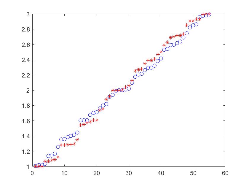
Figure 1: Generalized eigenvalues (blue circles) and nodal values of $r(x,y)$ (red asterisks) computed with the coarse mesh displayed in Fig. 2.

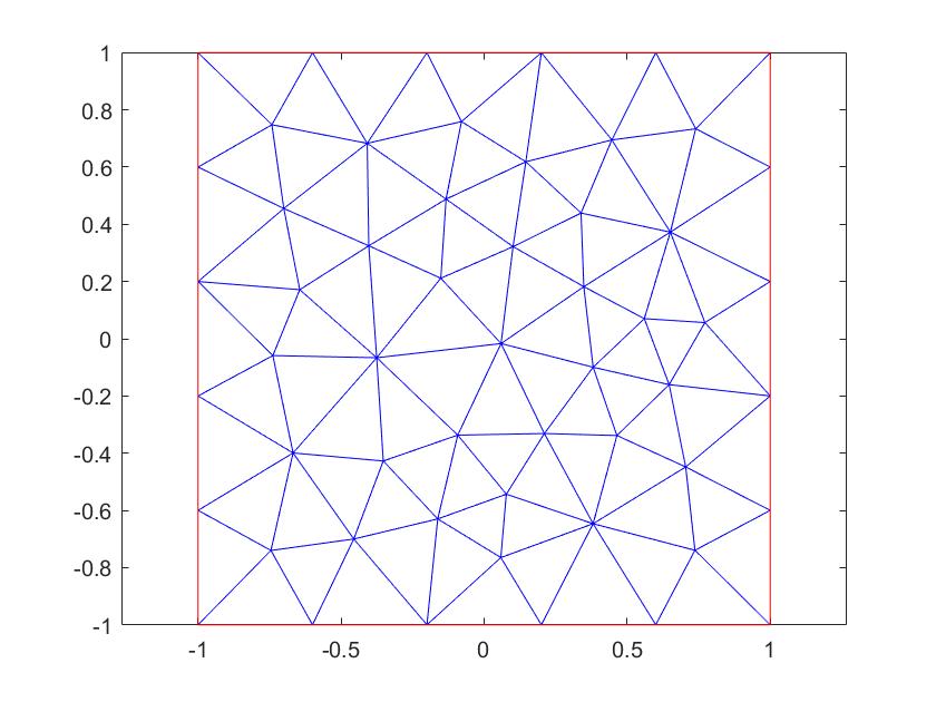
Figure 2: Matlab’s grid, coarse case.

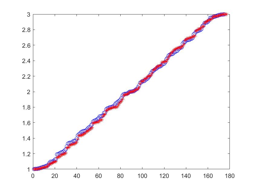
Figure 3: Generalized eigenvalues (blue circles) and nodal values of $r(x,y)$ (red asterisks) computed with the “fine” mesh displayed in Fig. 4.

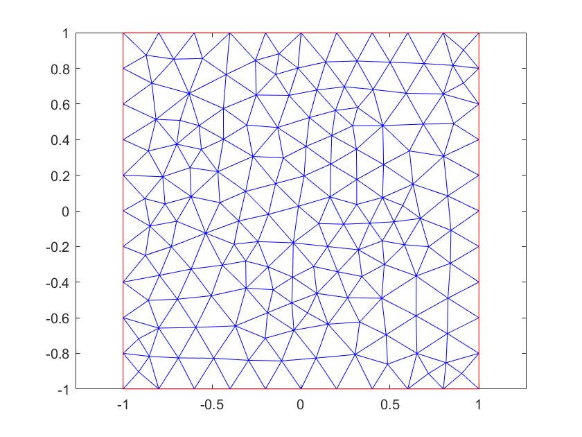
Figure 4: Matlab’s grid, “fine” case.

6 Conclusions and further work.

We have not only extended our earlier results [14, 7, 8], addressing Laplacian preconditioning, to preconditioners defined in terms of more general elliptic differential operators, but we have also proved that the entire spectrum of any operator in the form ${\mathcal{B}}^{-1}{\mathcal{A}}$ can be approximated with arbitrary accuracy by the eigenvalues of the associated discretized mappings. Here, ${\mathcal{A},B}:V\mapsto V^{\#}$ are linear, bounded, coercive and self-adoint operators defined on an infinite dimensional Hilbert space $V$, and $V^{\#}$ denotes the dual space. Our analysis differs significantly from the classical investigations of the point spectrum of second order differential operators, which is typically done within the framework of compact (solution) operators.

In our opinion, these results yield a new perspective on the continuous spectrum of preconditioned elliptic differential operators, and there are several unanswered questions: For example, are the results presented in section 3 also valid if the coefficient functions $k(x)$ and $g(x)$ are replaced by symmetric and uniformly positive definite conductivity tensors $K(x)$ and $G(x)$, respectively? Also, and perhaps even more interesting, do Theorem 4.2 and Corollary 4.3 also hold for more general continuously invertible operators ${\mathcal{A}}:V\mapsto V^{\#}$, e.g., for saddle point problems?

Appendix A Approximations of the spectrum of self-adjoint operators.

Using [3, Chapter 3] and [11, Chapter 8], we first recall several results concerning the convergence of linear self-adjoint operators defined on infinite dimensional Hilbert spaces. By the Hellinger-Toeplitz theorem (see [5, Theorem 5.7.2, p. 260]), any linear self-adjoint operator ${\mathcal{Z}}:V\mapsto V$ on a Hilbert space $V$ is closed and, according to the Banach closed-graph theorem, bounded (continuous).

Consider a bounded linear operator ${\mathcal{G}}:V\mapsto V$ (not necessarily self-adjoint, therefore we for the moment change the notation) and a sequence of its bounded linear approximations $\{{\mathcal{G}}_{n}\},{\mathcal{G}}_{n}:V\mapsto V$, that can converge to ${\mathcal{G}}$ in different ways:

• pointwise (strongly), i.e.,   ${\mathcal{G}}_{n}\stackrel{{\scriptstyle p}}{{\rightarrow}}{\mathcal{G}}$

  $$\mbox{iff for all}\;x\in V,\quad\lim_{n\rightarrow\infty}\|{\mathcal{G}}x-{\mathcal{G}}_{n}x\|=0\,;$$

• uniformly (in norm), iff   $\lim_{n\rightarrow\infty}\|{\mathcal{G}}-{\mathcal{G}}_{n}\|=0\,;$

• stably, i.e.   ${\mathcal{G}}_{n}\stackrel{{\scriptstyle s}}{{\rightarrow}}{\mathcal{G}}$   iff

  • ${\mathcal{G}}_{n}\stackrel{{\scriptstyle p}}{{\rightarrow}}{\mathcal{G}}$, and

  • the inverse operators   $\{{\mathcal{G}}_{n}^{-1}\}$   are uniformly bounded, i.e., for some $C>0$, $\|{\mathcal{G}}_{n}^{-1}\|\leq C$ for all $n$.

Clearly, uniform convergence implies pointwise convergence, but the converse implication does not hold. Since the class of compact operators is closed with respect to uniform convergence, the uniform convergence concept can not be used to investigate the convergence of compact to non-compact operators, such as to bounded continuously invertible operators defined on infinite dimensional Hilbert spaces.

The spectral theory for bounded linear operators is based on the concept of the operator resolvent

$${\mathcal{R}}(\mu):=(\mu\mathcal{I}-\mathcal{G})^{-1}$$

and on the resolvent set

$$\rho({\mathcal{G}}):=\left\{\mu\in\mathbb{C};\,\mu\mathcal{I}-\mathcal{G}\;\mbox{has a bounded inverse}\right\}.$$ (42)

It is interesting to notice that, for any $\mu\in\rho({\mathcal{G}})$, a sequence of shifted operators $\{\mu\mathcal{I}-\mathcal{G}_{n}\}$ converge to $\mu\mathcal{I}-\mathcal{G}$ stably if, and only if, $\{\mathcal{G}_{n}\}$ and the resolvents $\{{\mathcal{R}}_{n}(\mu)\},{\mathcal{R}}_{n}(\mu):=(\mu\mathcal{I}-\mathcal{G}_{n})^{-1}$, converge to $\mathcal{G}$ and ${\mathcal{R}}(\mu)$ pointwise, respectively, i.e.,

$$\mu\mathcal{I}-\mathcal{G}_{n}\stackrel{{\scriptstyle s}}{{\rightarrow}}\mu\mathcal{I}-\mathcal{G}\quad\mbox{iff}\quad\mathcal{G}_{n}\stackrel{{\scriptstyle p}}{{\rightarrow}}\mathcal{G}\;\mbox{and}\;{\mathcal{R}}_{n}(\mu)\stackrel{{\scriptstyle p}}{{\rightarrow}}{\mathcal{R}}(\mu).$$ (43)

Indeed, using the resolvent identity

$${\mathcal{R}}_{n}(\mu)-{\mathcal{R}}(\mu)={\mathcal{R}}_{n}(\mu)\,({\mathcal{G}}_{n}-{\mathcal{G}})\,{\mathcal{R}}(\mu),$$

the right implication follows immediately from the definition of stable convergence. Conversely, from the pointwise convergence of ${\mathcal{R}}_{n}(\mu)$ and the uniform boundedness principle (Banach–Steinhaus theorem) we conclude that $\{{\mathcal{R}}_{n}(\mu)\}=\{(\mu\mathcal{I}-\mathcal{G}_{n})^{-1}\}$ is uniformly bounded and the result follows.

We will now present the proof of Theorem 4.1; cf. also [11, chapter VIII, § 1.2, Theorem 1.14, p. 431] and [3, chapter 5, section 4, Theorem 5.12, p. 239-240].

Theorem A.1 (Approximation of the spectrum of self-adjoint operators).

Let ${\mathcal{Z}}$ be a linear self-adjoint operator on a Hilbert space $V$ and let $\{{\mathcal{Z}}_{n}\}$ be a sequence of linear self-adjoint operators on $V$ converging to ${\mathcal{Z}}$ pointwise (strongly). Then, for any point $\lambda\in\mathrm{sp}({\mathcal{Z}})$ in the spectrum of ${\mathcal{Z}}$, and for any of its neighbourhoods, there exists ${\mathcal{Z}}_{j}$ such that the intersection of its spectrum $\mathrm{sp}({\mathcal{Z}}_{j})$ with this neighbourhood is nonempty.

Proof.

Consider any point $\lambda\in\mathrm{sp}({\mathcal{Z}})\subset\mathbb{R}$ in the spectrum of ${\mathcal{Z}}$. Then, for any $\varepsilon>0$, the point $\mu:=\lambda+\iota\varepsilon$, where $\iota$ is the complex unit, belongs to the resolvent set $\rho({\mathcal{Z}})$ (because ${\mathcal{Z}}$ is self-adjoint). For self-adjoint operators, the norm of the resolvent at any point in the resolvent set is equal to the inverse of the distance of the given point to the spectrum (see, e.g., [3, Proposition 2.32]). Therefore, for all $n$,

$$\|{\mathcal{R}}(\mu)\| :=\|(\mu\mathcal{I}-\mathcal{Z})^{-1}\|=\frac{1}{\mathrm{dist}(\mu,\mathrm{sp}({\mathcal{Z}}))}=\frac{1}{\varepsilon}\,,$$ (44)

$$\|{\mathcal{R}}_{n}(\mu)\| :=\|(\mu\mathcal{I}-\mathcal{Z}_{n})^{-1}\|=\frac{1}{\mathrm{dist}(\mu,\mathrm{sp}({\mathcal{Z}}_{n}))}\leq\frac{1}{\varepsilon}\,.$$ (45)

The inequality in (45) follows from the assumption that $\{{\mathcal{Z}}_{n}\}$ is a sequence of self-adjoint operators, i.e., $\mathrm{sp}({\mathcal{Z}}_{n})\subset\mathbb{R}$. Note that inequality (45) provides the uniform boundedness of $\{{\mathcal{R}}_{n}(\mu)\}$, which, together with the pointwise convergence of $\{{\mathcal{Z}}_{n}\}$, yields that

$$\mu{\mathcal{I}}-{\mathcal{Z}}_{n}\stackrel{{\scriptstyle s}}{{\rightarrow}}\mu{\mathcal{I}}-{\mathcal{Z}}.$$

Using (43), we thus have the pointwise convergence of $\{{\mathcal{R}}_{n}(\mu)\}$, i.e., for any $x\in V,||x\|=1,$

$$\|{\mathcal{R}}(\mu)x\|=\lim_{n\rightarrow\infty}\|{\mathcal{R}}_{n}(\mu)x\|.$$

Consider a fixed $x\in V,||x\|=1,$ such that

$$\frac{1}{2\varepsilon}\leq\|{\mathcal{R}}(\mu)x\|\leq\frac{1}{\varepsilon}.$$

(The existence of such a $x\in V$ follows from (44).) Then, from the pointwise convergence, there must exist $n$ such that

$$\|{\mathcal{R}}_{n}(\mu)\|\geq\|{\mathcal{R}}_{n}(\mu)x\|\geq\frac{1}{3\varepsilon}.$$

Recall that $\|{\mathcal{R}}_{n}(\mu)\|=\mathrm{[dist}(\mu,\mathrm{sp}({\mathcal{Z}}_{n}))]^{-1}$. Therefore there exists a point $\lambda_{n}\in\mathrm{sp}({\mathcal{Z}}_{n})$ such that

$$|\lambda_{n}-\mu|\leq 3\varepsilon\quad\mbox{and, consequently,}\quad|\lambda_{n}-\lambda|\leq 4\varepsilon,$$

which finishes the proof. ∎

References

• [1] D. N. Arnold, R. S. Falk, and R. Winther. Finite element exterior calculus: from Hodge theory to numerical stability. Bull. Amer. Math. Soc. (N.S.), 47:281–354, 2010.
• [2] J. A. Bondy and U. S. R. Murty. Graph theory with applications. American Elsevier Publishing Co., Inc., New York, 1976.
• [3] Françoise Chatelin. Spectral approximation of linear operators. Academic Press, New York, 1983.
• [4] Philippe G. Ciarlet. The finite element method for elliptic problems, volume 40 of Classics in Applied Mathematics. Society for Industrial and Applied Mathematics (SIAM), Philadelphia, PA, 2002. Reprint of the 1978 original [North-Holland, Amsterdam; MR0520174 (58 #25001)].
• [5] Philippe G. Ciarlet. Linear and nonlinear functional analysis with applications. Society for Industrial and Applied Mathematics, Philadelphia, PA, 2013.
• [6] J. Descloux, N. Nassif, and J. Rappaz. On spectral approximation. part 1. the problem of convergence. RAIRO - Analyse numérique, 12:97–112, 1978.
• [7] T. Gergelits, K. A. Mardal, B. F. Nielsen, and Z. Strakoš. Laplacian preconditioning of elliptic PDEs: Localization of the eigenvalues of the discretized operator. SIAM Journal on Numerical Analysis, 57(3):1369–1394, 2019.
• [8] T. Gergelits, B. F. Nielsen, and Z. Strakoš. Generalized spectrum of second order differential operators. SIAM Journal on Numerical Analysis, 58(4):2193–2211, 2020.
• [9] Tomáš Gergelits. Krylov Subspace Methods: Analysis and Applications. PhD thesis, Charles University, 2020.
• [10] I. Pultarová J. Hrnčíř and Z. Strakoš. Decomposition of subspaces preconditioning: abstract framework. Numerical Algorithms, 83:57–98, 2020.
• [11] Tosio Kato. Perturbation Theory for Linear Operators. Springer-Verlag, Berlin Heidelberg, 1980.
• [12] I. Pultarová M. Ladecký and J. Zeman. Guaranteed two-sided bounds on all eigenvalues of preconditioned diffusion and elasticity problems solved by the finite element method. Applications of Mathematics, 2020.
• [13] Josef Málek and Zdeněk Strakoš. Preconditioning and the conjugate gradient method in the context of solving pdes. SIAM Spotlight Series, December 2014.
• [14] B. F. Nielsen, A. Tveito, and W. Hackbusch. Preconditioning by inverting the Laplacian; an analysis of the eigenvalues. IMA Journal of Numerical Analysis, 29(1):24–42, 2009.
• [15] G. W. Stewart and Ji Guang Sun. Matrix perturbation theory. Computer Science and Scientific Computing. Academic Press, Inc., Boston, MA, 1990.
• [16] Yu. V. Vorobyev. Methods of Moments in Applied Mathematics. Translated from the Russian by Bernard Seckler. Gordon and Breach Science Publishers, New York, 1965.