A new minimizing-movements scheme
for curves of maximal slope

Abstract.

Curves of maximal slope are a reference gradient-evolution notion in metric spaces and arise as variational formulation of a vast class of nonlinear diffusion equations. Existence theories for curves of maximal slope are often based on minimizing-movements schemes, most notably on the Euler scheme. We present here an alternative minimizing-movements approach, yielding more regular discretizations, serving as a-posteriori convergence estimator, and allowing for a simple convergence proof.

1. Introduction

Gradient-flow evolution in metric spaces has been the subject of intense research in the last years. Starting from the pioneering remarks in [18], the theory has been boosted by the monograph by Ambrosio, Gigli, & Savaré [5] and now encompasses existence and approximation results, as well as long-time behavior, decay to equilibrium, and regularity [37].

The applicative interest in evolution equations in metric spaces has been revived by the seminal observations in [22] and the work by Otto [30] that a remarkably large class of diffusion equations can be variationally reinterpreted as gradient flows in Wasserstein spaces. More precisely, consider the nonlinear diffusion equation

$$\partial_{t}\rho-{\rm div}\big{(}\rho\nabla(V+F^{\prime}(\rho)+W\ast\rho)\big{)}=0\quad\text{in}\ \mathbb{R}^{d}\times(0,T).$$ (1.1)

Here, $\rho=\rho(x,t)\geq 0$ is a time-dependent density with fixed total mass $\int_{\mathbb{R}^{d}}\rho(x,t)\,{\rm d}x=1$ and finite second moment $\int_{\mathbb{R}^{d}}|x|^{2}\rho(x,t)\,{\rm d}x<\infty$. Finally, $V:\mathbb{R}^{d}\to\mathbb{R}$ is a confinement potential, $F:[0,\infty)\to\mathbb{R}$ is an internal-energy density, $W:\mathbb{R}^{d}\to\mathbb{R}$ is an interaction potential, and $\ast$ stands for the standard convolution in $\mathbb{R}^{d}$.

Equation (1.1) can be variationally reformulated in terms of the gradient flow in the metric space $(\mathcal{P}_{2}(\mathbb{R}^{d}),W_{2})$ of probability measures with finite second moment endowed with the $2$-Wasserstein distance $W_{2}$ of the functional $\phi$ defined as

$$\phi(u)=\int_{\mathbb{R}^{d}}V(x)\,{\rm d}u(x)+\int_{\mathbb{R}^{d}}F(\rho(x))\,{\rm d}x+\frac{1}{2}\int_{\mathbb{R}^{d}\times\mathbb{R}^{d}}W(x{-}y)\,{\rm d}(u\otimes u)(x,y)$$ (1.2)

if $u=\rho{\mathcal{L}}^{d}$ and $\phi(u)=\infty$ if $u$ is not absolutely continuous with respect to the Lebesgue measure ${\mathcal{L}}^{d}$ in $\mathbb{R}^{d}$ see [5] and Section 8.

The reference notion of solution to gradient flows in metric spaces is that of curves of maximal slope [18], see Definition 2.1 below. This is based on a specific reformulation of (1.1) in form of a single scalar relation, featuring specific scalar quantities playing the role of the norm of time derivative of the trajectory and of the gradient of the energy, in the spirit of (1.4) below. Existence and decay to equilibrium of curves of maximal slope for $\phi$ in $(\mathcal{P}_{2}(\mathbb{R}^{d}),W_{2})$ are available, see [5, 11, 12], for instance.

In this paper, we focus on a novel time-discretization scheme for gradient flows in metric spaces, falling within the class of Minimizing Movements in the sense of De Giorgi [4, 17]. Our theory is framed in abstract metric spaces, see Sections 2-5, and applied in linear and Wasserstein spaces in Sections 7 and 8, respectively. To keep this introductory discussion as simple as possible, we present here the idea in the case of the doubly nonlinear ODE system driven by a smooth potential $\phi$ on $\mathbb{R}^{d}$, namely

$$|u^{\prime}|^{p-2}u^{\prime}+\nabla\phi(u)=0\quad\text{in}\ \times(0,T)$$ (1.3)

for $p>1$, where the prime denotes time differentiation. This equation can be equivalently rewritten as

$$\phi(u(t))+\frac{1}{p}\int_{0}^{t}|u^{\prime}(r)|^{p}{\rm d}r+\frac{1}{q}\int_{0}^{t}|\nabla\phi(u(r))|^{q}{\rm d}r-\phi(u(0))=0\quad\forall t\in(0,T)$$ (1.4)

where now $q=p/(p-1)$ is conjugate to $p$. Note that the left-hand side above is always nonnegative, so that (1.4) corresponds indeed to a so-called null-minimization principle: the left-hand side is minimized and one checks that the minimum value is $0$. This approach has been lately referred to as De Giorgi’s Energy-Dissipation principle and has already been applied in a variety of different contexts, including generalized gradient flows [8, 34], rate-independent [27, 32] and GENERIC systems [19, 24], and optimal control [31].

We complement equation (1.3) by specifying the initial condition $u(0)=u^{0}$ for some $u^{0}\in\mathbb{R}^{d}$. By introducing a time partition of $(0,T)$ with uniform steps $\tau=T/N>0$, $N\in\mathbb{N}$ (note however that we consider nonuniform partitions below), and letting $u_{0}=u^{0}$, the new minimizing-movements scheme reads

$$u_{i}\in{\rm arg\,min}_{u}\left(\phi(u)+\frac{\tau^{1-p}}{p}\left|{u-u_{i-1}}\right|^{p}+\frac{\tau}{q}|\nabla\phi(u)|^{q}-\phi(u_{i-1})\right)$$ (1.5)

for $i=1,\dots,N$. With respect to the classical implicit Euler method, scheme (1.5) includes an extra term featuring the norm of the gradient. This modification with respect to Euler makes the function to be minimized in (1.5) a discrete and localized version of the left-hand side in (1.4). As such, scheme (1.5) is nothing by the canonical variational integrator scheme [21] associated with the De Giorgi’s Energy-Dissipation principle.

Compared to Euler, the new minimizing-movements scheme (1.5) shows some distinguishing features. First of all, the direct occurrence of the gradient in (1.5) entails additional regularity of discrete solutions, see (3.11). As a matter of illustration, in the case of the linear heat equation ($p=2$) with homogeneous Dirichlet boundary conditions scheme (1.5) corresponds to solving the problem

$$\frac{u_{i}-u_{i}}{\tau}-\Delta u_{i}+\tau\Delta^{2}u_{i}=0,$$

which is reminiscent of a singular perturbation of the Euler scheme, see Section 3.3.

Secondly, the exact correspondence of (1.5) to the left-hand side of (1.4) allows to check convergence of discrete solutions without the need of introducing the so-called De Giorgi’s variational interpolation function [5, Def. 3.2.1].

Thirdly, in using a time discretization to detect a minimum point of $\phi$ by iterating on the time steps, the new scheme shows enhanced performance with respect to Euler for large time steps, see [24] and (3.20) below.

Finally, the functional under minimization in (1.5) may serve as an a-posteriori estimator for the convergence of any discrete solution, regardless of the specific method used to obtain it. In particular, one can resort to approximate minimizers instead of true minimizers.

The minimizing-movements scheme (1.5) was already analyzed in [24] in the case of gradient flows in Hilbert spaces. In particular, convergence of the scheme for $\phi$ being a $C^{1,\alpha}$ perturbation of a convex function and sharp, order-one error estimates in finite dimensions can be found there. The case of curves of maximal slope in metric spaces is also mentioned in [24], where nevertheless the analysis is limited to $p=2$ and geodesically convex potentials.

In this note, we extend the analysis of [24] to the case $p>1$ and to potentials $\phi$ being $(\lambda,p)$-generalized-geodesically convex for $\lambda\in\mathbb{R}$. More precisely, the combination of our main results, Theorems 3.1-3.2, entails that solutions to the new minimizing-movements scheme (1.5) in metric spaces, see (3.2), converge to curves of maximal slope for all $p>1$, if $\lambda\geq 0$, and for $p>2$, if $\lambda<0$.

In addition, in Theorem 3.3 we are able to provide a convergence result for not geodesically convex functionals, provided that some weak differentiability of its slope in form of a generalized one-sided Taylor expansion condition holds, see (3.13).

Before closing this introduction let us mention that alternative time-discrete scheme with respect to Euler are available, also in the nonlinear setting of metric spaces [15, 26, 25, 38]. We postpone an account on the literature to Subsection 3.4, for some preliminary material is needed to put these contributions in perspective.

This is the plan of the paper. We introduce some notation and preliminaries in Section 2 and present our main convergence results in Section 3. In particular, assumptions are collected in Subsection 3.1 and statements are given in Subsection 3.2. Some illustration of the theory on two linear equations, both in finite and infinite dimensions, is in Subsection 3.3. The convergence results are then proved in Sections 4-6. Eventually, we comment on the application of the abstract theory in linear spaces in Section 7 and in Wasserstein spaces in Section 8.

2. Preliminaries

We briefly collect here some classical notation and preliminaries on evolution in metric spaces, for completeness. The reader familiar with the classical reference [5] may consider moving directly to Section 3.

In all of the following, $(U,d)$ denotes a complete metric space and $\phi:U\to(-\infty,\infty]$ is a proper functional, i.e., the effective domain $D(\phi):=\{u\in U\ :\ \phi(u)<\infty\}$ is assumed to be nonempty.

Let $p,\,q>1$ be given with $1/p+1/q=1$. A curve $u:[0,T]\to U$ is said to belong to $AC^{p}([0,T];U)$ if there exists $m\in L^{p}(0,T)$ with

$$d(u(s),u(t))\leq\int_{s}^{t}m(r)\,{\rm d}r\quad\text{for all \ $0\leq s\leq t<T.$}$$ (2.1)

If $u\in AC^{p}([0,T];U)$, the limit

$$|u^{\prime}|(t):=\lim_{s\to t}\frac{d(u(s),u(t))}{|t-s|}$$

exists for almost everywhere $t\in(0,T)$, see [5, Thm. 1.1.2], and is referred to as metric derivative of $u$ at $t$. Moreover, the map $t\mapsto|u^{\prime}|(t)$ is in $L^{p}(0,T)$ and is minimal within the class of functions $m\in L^{p}(0,T)$ fulfilling (2.1).

The local slope [5, 13, 18] of $\phi$ at $u\in D(\phi)$ is defined via

$$|\partial\phi|(u):=\limsup_{v\to u}\frac{(\phi(u)-\phi(v))^{+}}{d(u,v)}.$$

If $U$ is a Banach space and $\phi$ is Fréchet differentiable, we have that $|\partial\phi|(u)=\|{\rm D}\phi(u)\|_{*}$ (dual norm).

In the following, we will make use of the notion of geodesic convexity for $\phi$. More precisely, we call (constant-speed) geodesic any curve $\gamma:[0,1]\to U$ such that $d(\gamma(t),\gamma(s))=(t-s)d(\gamma(0),\gamma(1))$ for all $0\leq s\leq t\leq T$ and we say that $\phi$ is $(\kappa,p)$-geodesically convex for $\kappa\in\mathbb{R}$ if for all $v_{0},\,v_{1}\in D(\phi)$ there exists a geodesic with $\gamma(0)=v_{0}$ and $\gamma(1)=v_{1}$ such that

$$\phi(\gamma(\theta))\leq\theta\phi(v_{1})+(1-\theta)\phi(v_{0})-\frac{\kappa}{p}\theta(1-\theta)d^{p}(v_{0},v_{1})\ \ \forall\theta\in[0,1]$$ (2.2)

The definition is classical for $p=2$. For this $p$-extension see [5, Remark. 2.4.7] or [1]. Note that geodesic convexity in particular implies that $U$ is a geodesic space, for each pair $v_{0}$, $v_{1}$ is connected by a geodesic. More generally, we say that $\phi$ is $(\kappa,p)$-generalized-geodesically convex if (2.2) holds for some curve $\gamma$ connecting $v_{0}$ and $v_{1}$, not necessarily being a geodesic. In this case, $U$ is implicitly assumed to be path-connected.

From [35, Prop. 2.7] we have that if $\phi$ is $(\kappa,p)$-geodesically convex and $d$-lower semicontinuous, the local slope $|\partial\phi|$ is $d$-lower semicontinuous as well. In addition, $|\partial\phi|$ admits the representation

$$|\partial\phi|(u)=\sup_{v\neq u}\left(\frac{\phi(u)-\phi(v)}{d(u,v)}+\frac{\kappa}{p}d^{p-1}(u,v)\right)^{+}\quad\forall u\in D(\phi).$$ (2.3)

We denote by $D(|\partial\phi|)$ the effective domain of $|\partial\phi|$, namely, $D(|\partial\phi|)=\{u\in D(\phi)\ :\ |\partial\phi|(u)<\infty\}$. Under the above-mentioned geodesic convexity assumption, the local slope $|\partial\phi|$ is a strong upper gradient [5, Def. 1.3.2]. Namely, for all $u\in AC^{p}([0,T];U)$, the map $r\mapsto|\partial\phi|(r)$ is Borel and

$$|\phi(u(t))-\phi(u(s))|\leq\int_{s}^{t}|\partial\phi|(u(r))\,|u^{\prime}|(r)\,{\rm d}r\quad\forall 0\leq s\leq t\leq T.$$

Note that, if $r\mapsto|\partial\phi|(u(r))|u^{\prime}|(r)\in L^{1}(0,T)$ the latter entails that $\phi\circ u\in W^{1,1}(0,T)$ and $(\phi\circ u)^{\prime}=|\partial\phi|(u)|u^{\prime}|$ almost everywhere in $(0,T)$.

Along with the above provisions, we specify the notion of gradient-driven evolution as follows.

Definition 2.1 (Curve of maximal slope).

The trajectory $u\in AC^{p}([0,T];U)$ is said to be a curve of maximal slope if $\phi\circ u\in W^{1,1}(0,T)$ and

$$\phi(u(t))+\frac{1}{p}\int_{0}^{t}|u^{\prime}|^{p}(r)\,{\rm d}r+\frac{1}{q}\int_{0}^{t}|\partial\phi|^{q}(u(r))\,{\rm d}r=\phi(u(0))\quad\forall t\in[0,T].$$ (2.4)

3. Main results

To each time partition $0=t_{0}<t_{1}<\dots<t_{N}=T$ we associate the time steps $\tau_{i}=t_{i}-t_{i-1}$ and the diameter $\tau=\max\tau_{i}$. Given the vector $\{u_{i}\}_{i=0}^{N}\in U^{N+1}$ we define its backward piecewise constant interpolant $\overline{u}:[0,T]\to U$ on the time partition to be

$$\overline{u}(0)=u_{0}\quad\text{and}\quad\overline{u}(t)=u_{i}\quad\forall t\in(t_{i-1},t_{i}],\ i=1,\dots,N.$$

Moreover, we define the piecewise constant function $|\widehat{u}^{\prime}|:[0,T]\setminus\{t_{0},\dots,t_{N}\}\to[0,\infty)$ as

$$|\widehat{u}^{\prime}|(t):=\frac{d(u_{i-1},u_{i})}{\tau_{i}}\quad\forall t\in(t_{i-1},t_{i}),\ i=1,\dots,N.$$

The notation $|\widehat{u}^{\prime}|(t)$ alludes to the fact that in the Hilbert-space case the latter is nothing but the norm of the time derivative of the piecewise affine interpolant of the values $\{u_{i}\}_{i=0}^{N}$ on the time partition.

Our new minimizing-movements scheme is specified by means of the incremental functional $G:(0,\infty)\times D(\phi)\times D(|\partial\phi|)$ given by

$$\boxed{G(\tau,v,u):=\phi(u)+\frac{\tau^{1-p}}{p}d^{p}(v,u)+\frac{\tau}{q}|\partial\phi|^{q}(u)-\phi(v).}$$ (3.1)

In the setting of the assumptions specified later in Subsection 3.1, for all $(\tau,v)\in(0,\infty)\times D(\phi)$ the functional $u\in D(|\partial\phi|)\mapsto G(\tau,v,u)$ admits a minimizer, possibly being not unique. We indicate the set of such minimizers by $M_{G}(\tau,v)$ and the minimum value of $G(\tau,v,\cdot)$ by $\widehat{G}(\tau,v)$, namely,

$$M_{G}(\tau,v):={\rm arg\,min}_{u\in D(|\partial\phi|)}G(\tau,v,u),\quad\widehat{G}(\tau,v):=\min_{u\in D(|\partial\phi|)}G(\tau,v,u).$$

With this notation, the new minimizing-movements scheme reads

$$\boxed{u_{0}=u^{0}\ \ \text{and}\ \ u_{i}\in M_{G}(\tau_{i},u_{i-1})\quad\text{for}\ i=1,\dots,N,}$$ (3.2)

for some given initial datum $u^{0}\in D(\phi)$.

For later purposes, we introduce also the incremental functional $E:(0,\infty)\times D(\phi)\times D(\phi)$ associated with the classical backward Euler method

$$E(\tau,v,u):=\phi(u)+\frac{\tau^{1-p}}{p}d^{p}(v,u)-\phi(v),$$ (3.3)

as well as the corresponding notation

$$M_{E}(\tau,v):={\rm arg\,min}_{u\in D(\phi)}E(\tau,v,u),\quad\widehat{E}(\tau,v):=\min_{u\in D(\phi)}E(\tau,v,u).$$

In particular, the Euler method corresponds to the incremental problem

$$u_{0}=u^{0}\ \ \text{and}\ \ u_{i}\in M_{E}(\tau_{i},u_{i-1})\quad\text{for}\ i=1,\dots,N.$$ (3.4)

In the context of Wasserstein spaces, see Section 8, the latter is often referred to as Jordan-Kinderlehrer-Otto scheme [22].

3.1. Assumptions

In this subsection, we fix our assumptions and collect some comment. We start by asking that

$$(U,d)\ \ \text{is a complete metric space}.$$ (3.5)

In addition to the metric topology, $(U,d)$ is assumed to be endowed with

$$\text{a Hausdorff topology}\ \sigma,\ \text{compatible with the metric $d$}.$$ (3.6)

The latter compatibility is intended in the following sense

$$u_{n}\stackrel{{\scriptstyle\sigma}}{{\to}}u,\ v_{n}\stackrel{{\scriptstyle\sigma}}{{\to}}v\ \ \Rightarrow\ \ d(u,v)\leq\liminf_{n\to\infty}d(u_{n},v_{n})$$ (3.7)

and, in essence, means that $\sigma$ is weaker than the topology induced by $d$. An early example for $\sigma$ complying with (3.6) is the topology induced by $d$. In applications it may however be useful to keep the two topologies separate. In particular, if $U$ is a Banach space $\sigma$ is often chosen to be some weak topology whereas $d$ usually corresponds to the strong one.

The initial datum is assumed to satisfy

$$u^{0}\in D(\phi).$$ (3.8)

We assume the proper potential $\phi:U\to(-\infty,\infty]$ to be such that

$$\text{the sublevels of $\phi$ are sequentially $\sigma$-compact}.$$ (3.9)

The latter in particular entails that $\phi$ is sequentially $\sigma$-lower semicontinuous and bounded from below. In the following, we hence assume with no loss of generality that $\phi$ is nonnegative. Note however that assumption (3.9) could be weakened by asking compactness on $d$-bounded sublevels of $\phi$ only.

In addition, we ask that

$$|\partial\phi|\ \text{is a strong upper gradient for $\phi$ and it is sequentially}$$

$$\sigma d \phi$$-lower semicontinuous on -bounded sublevels of . (3.10)

The latter assumption could be weakened by developing the theory for some relaxation of $|\partial\phi|$. Still, [35, Prop. 2.7] ensures that (3.10) hold, as soon as $\phi$ is $(\lambda,p)$-geodesically convex and $\sigma$ is the metric topology induced by $d$.

In the setting of assumptions (3.5)-(3.10), the solvability of the incremental minimization problem (3.2) follows from the Direct Method. Indeed, for all $\tau>0$ and $v\in D(\phi)$ the incremental functional $u\in D(|\partial\phi|)\mapsto G(\tau,v,u)$ is coercive and lower semicontinuous by (3.9)-(3.10). We will later check in (6.7) that indeed

$$u\in M_{G}(\tau,v)\ \ \Rightarrow\ \ |\partial(\phi+\tau|\partial\phi|^{q}/q)|(u)<\infty.$$ (3.11)

In particular, minimizers of $G(\tau,v,\cdot)$ show additional regularity. This extra regularity may be not preserved by the time-continuous limit.

Under the sole (3.9) the incremental Euler minimization problem (3.4) is solvable as well. In particular, for all $\tau>0$ and $v\in D(\phi)$ the functional $u\in D(\phi)\mapsto E(\tau,v,u)$ admits a minimizer.

Along the analysis, we will make reference to specific generalized geodesically convex cases. In particular, we may ask for

$$\exists\tau_{*}>0,\ \lambda\in\mathbb{R}\ \ \text{such that}\ \ \forall\tau\in(0,\tau_{*}),\ \forall v\in D(\phi)$$

$$u\mapsto E(\tau,v,u)\ \ \text{is $(\kappa,p)$-generalized-geodesically convex}$$

$$\text{with $\kappa=(p-1)\tau^{1-p}+\lambda$}.$$ (3.12)

Note that (3.12) holds if $\phi$ is $(\lambda,p)$-geodesically convex and the $p$-power of the distance is $(p-1,p)$-geodesically convex. In case $p=2$, the $(1,2)$-geodesic convexity of $u\mapsto d^{2}(u,v)/2$ qualifies nonpositively curved spaces in the Alexsandrov sense [3, 23]. In particular, Euclidean and Hilbert spaces, as well as Riemannian manifolds of nonpositive sectional curvature [5, Rem. 4.0.2] fall into this class.

Condition (3.12) is more demanding for $p\not=2$. In fact, by letting $\tau\to 0$ it implies that the $p$-power of the distance is $(p-1,p)$-geodesically convex. This is actually not the case in linear spaces, as one can check already in $\mathbb{R}$, but see also [2, Lem. 3.1]. Indeed, let $\theta=1/2$ and $v_{0}=-1$, $v_{1}=1$, $\theta=1/2$ for $p>2$ and $v_{0}=0$, $v_{1}=1$ for $p<2$ in order to get

$$\frac{1}{p}|\theta v_{1}+(1-\theta)v_{0}|^{p}>\frac{\theta}{p}|v_{1}|^{p}+\frac{1-\theta}{p}|v_{0}|^{p}-\theta(1-\theta)\frac{p-1}{p}|v_{1}-v_{0}|^{p}$$

contradicting $(p-1,p)$-geodesic convexity. See [23, Ex. 1, p. 55] for some similar argument, proving the failure of $(1,2)$-geodesic convexity of $(x_{1},x_{1})\in\mathbb{R}^{2}\mapsto(x_{1}^{p}+x_{2}^{p})^{1/p}$. In fact, condition (3.12) for $p\not=2$ is actually meaningful only in spaces of qualified negative curvature. This is not the case for the Wasserstein space $(\mathcal{P}_{2}(\mathbb{R}^{d}),W_{2})$, which is actually of positive curvature, see Section 8. As we deal in Sections 7-8 with applications in linear and Wasserstein spaces, condition (3.12) is used there only for $p=2$.

In case of not geodesically convex potentials, we are still in the position of providing a convergence result under the following generalized one-sided Taylor-expansion condition on $|\partial\phi|$

$$\exists\tau_{*}>0,\,\forall C>0,\,\exists g:(0,\tau_{*})\to[0,\infty]\ \text{with}\ \frac{1}{\tau}\int_{0}^{\tau}g(r)\,{\rm d}r\searrow 0\ \text{as}\ \tau\to 0\ \text{such that}$$

$$\forall\tau\in(0,\tau_{*}),\ \forall v\in D(|\partial\phi|)\ \text{with}\ \max\{\phi(v),\tau|\partial\phi|^{q}(v)\}\leq C,\ \forall u\in M_{G}(\tau,v)$$

$$\text{we have that}\ \ |\partial\phi|^{q}(u)-|\partial(\phi+\tau|\partial\phi|^{q}/q)|^{q}(u)\leq g(\tau).$$ (3.13)

Notice that the last inequality makes sense, for we have the additional regularity (3.11). We discuss some applications fulfilling condition (3.13) in Sections 7 and 8.

A caveat on notation: In the following we use the same symbol $C$ in order to indicate a generic positive constant, possibly depending on data and changing from line to line. Where needed, dependencies are indicated by subscripts.

3.2. Convergence results

We are now ready to state our main results.

Theorem 3.1 (Conditional convergence).

Under (3.5)-(3.10) let $\{0=t_{0}^{n}<t_{1}^{n}<\dots<t^{n}_{N^{n}}=T\}$ be a sequence of partitions with $\tau^{n}:=\max(t^{n}_{i}-t^{n}_{i-1})\to 0$ as $n\to\infty$. Moreover, let $\{u_{i}^{n}\}_{i=0}^{N^{n}}$ be such that $u_{0}^{n}$ are $d$-bounded, $u_{0}^{n}\stackrel{{\scriptstyle\sigma}}{{\to}}u^{0}$, $\phi(u_{0}^{n})\to\phi(u^{0})$, and

$$\sum_{i=1}^{N^{n}}(G(\tau_{i}^{n},u_{i-1}^{n},u_{i}^{n}))^{+}\to 0\ \ \text{as}\ \ n\to\infty.$$ (3.14)

Then, up to a not relabeled subsequence, we have that $\overline{u}^{n}(t)\stackrel{{\scriptstyle\sigma}}{{\to}}u(t)$, where $u$ is a curve of maximal slope with $u(0)=u^{0}$.

Note that the statement of Theorem 3.1 does not require that $u^{n}_{i}\in M_{G}(\tau^{n}_{i},u^{n}_{i-1})$, namely that $\{u^{n}_{i}\}_{i=0}^{N^{n}}$ is a solution of the new minimizing-movements scheme (3.2). In particular, Theorem 3.1 can serve as an a-posteriori tool to check the convergence of time-discrete approximations, regardless of the method used to generate them. In particular, the above conditional convergence result directly applies to approximate minimizers, namely solutions of

$$u_{0}^{n}=u^{0}\quad\text{and}\quad G(\tau_{i},u^{n}_{i-1},u^{n}_{i})\leq\inf G(\tau_{i}^{n},u^{n}_{i-1},\cdot)+g^{n}_{i}\quad\text{for}\ i=1,\dots,N^{n}$$

(compare with (3.2)) as long as $\sum_{i=1}^{N^{n}}g^{n}_{i}\to 0$ as $n\to\infty$. See [20] for a result on approximate minimizers of $E(\tau_{i}^{n},u^{n}_{i-1},\cdot)$ instead.

The conditional convergence result of Theorem 3.1 thus relies on the possibility of solving the inequality $G(\tau_{i}^{n},u_{i-1}^{n},u_{i}^{n})\leq 0$ up to a small, controllable error, and establishing some a priori bounds on the discrete solution. The validity of condition (3.14) is to be checked on the specific problem at hand. In the specific case of $(\lambda,p)$-generalized-geodesically convex functionals $\phi$ on a properly nonpositively curved space, condition (3.14) actually holds for solutions of the new minimizing-movements scheme (3.2). This is the content of our second main result.

Theorem 3.2 (Convergence in the geodesically convex case).

Under assump- tions (3.5)-(3.10) and (3.12), let $\{0=t_{0}^{n}<t_{1}^{n}<\dots<t^{n}_{N^{n}}=T\}$ be a sequence of partitions with $\tau^{n}:=\max(t^{n}_{i}-t^{n}_{i-1})<\tau_{*}$ and $\tau^{n}\to 0$ as $n\to\infty$. Moreover, assume that either $\lambda\geq 0$ or $p>2$ in (3.12). Then, solutions $\{u_{i}^{n}\}_{i=0}^{N^{n}}$ of (3.2) fulfill condition (3.14). Hence, $\overline{u}^{n}$ converges pointwise to a curve of maximal slope up to subsequences.

We now turn to a convergence result in the not geodesically convex case. Here, some stronger topological assumption, an approximation of the initial datum, and the generalized one-sided Taylor-expansion assumption (3.13) for $|\partial\phi|$ are necessary.

Theorem 3.3 (Convergence without geodesic convexity).

Under assumptions (3.5)-(3.10), let $\sigma$ be the metric topology induced by $d$, $U$ be separable, and $\phi$ fulfill (3.13). Moreover, let $\{0=t_{0}^{n}<t_{1}^{n}<\dots<t^{n}_{N^{n}}=T\}$ be a sequence of partitions with $\tau^{n}:=\max(t^{n}_{i}-t^{n}_{i-1})<\tau_{*}$, $(\tau_{i}^{n}-\tau_{i-1}^{n})^{+}/\tau^{n}_{i-1}\leq C\tau^{n}$ for $i=2,\dots,N^{n}$, and $\tau^{n}\to 0$ as $n\to\infty$. Choose $u^{0n}\in M_{E}(\tau^{n},u^{0})$. Then, solutions $\{u_{i}^{n}\}_{i=0}^{N^{n}}$ of (3.2) with $u_{0}^{n}=u^{0n}$ fulfill condition (3.14). Hence, $\overline{u}^{n}$ converges pointwise to a curve of maximal slope up to subsequences.

Note that the one-sided nondegeneracy condition $(\tau_{i}^{n}-\tau_{i-1}^{n})^{+}/\tau^{n}_{i-1}\leq C\tau^{n}$ in the statement is fulfilled if $i\mapsto\tau^{n}_{i}$ in nonincreasing. In particular, it holds for uniform partitions. In case $u^{0}\in D(|\partial\phi|)$ no approximation of the initial datum as in Theorem 3.3 is actually needed.

Theorems 3.1, 3.2, and 3.3 are proved in Sections 4, 5, and 6, respectively.

3.3. An illustration on linear equations

The focus of our theory is on nonlinear problems. Still, as a way of illustrating the results, we present here two linear ODE and PDE examples. Nonlinear applications are then discussed in Sections 7-8 below.

Let us start from the finite-dimensional example of the gradient flow in $(\mathbb{R}^{d},|\cdot|)$ of $\phi(u)=\lambda|u|^{2}/2$ with $\lambda\in\mathbb{R}$ and take $p=2$. In this case, the incremental functional $G$ reads

$$G(\tau,v,u)=\frac{\lambda}{2}|u|^{2}+\frac{1}{2\tau}|u-v|^{2}+\frac{\tau\lambda^{2}}{2}|u|^{2}-\frac{\lambda}{2}|v|^{2}.$$

For all $v\in\mathbb{R}^{d}$ given, the latter can be readily minimized, giving the only minimum point $u=v/(1+\lambda\tau+\lambda^{2}\tau^{2})$. Correspondingly, the minimal value $\widehat{G}(t,v)$ can be checked to be

$$\widehat{G}(t,v)={}-\frac{|v|^{2}\lambda^{3}\tau^{2}}{2(1+\lambda\tau+\lambda^{2}\tau^{2})}.$$ (3.15)

If $\lambda\geq 0$ the minimal value is nonpositive and condition (3.14) trivially holds. If $\lambda<0$, the minimal value scales as $\tau^{2}$ and condition (3.14) still holds. Indeed, by letting

$$r^{n}:=\sum_{i=1}^{N^{n}}\big{(}G(\tau_{i}^{n},u_{i-1}^{n},u_{i}^{n})\big{)}^{+}$$ (3.16)

we have that

$$r^{n}=\sum_{i=1}^{N^{n}}\frac{|u_{i-1}^{n}|^{2}(\lambda^{-})^{3}(\tau_{i}^{n})^{2}}{2(1+\lambda\tau_{i}^{n}+\lambda^{2}(\tau_{i}^{n})^{2})}\leq C\max_{i}|u_{i}^{n}|^{2}\tau^{n}$$ (3.17)

where we tacitly assumed that $\lambda^{-}\tau^{n}\leq\lambda^{-}\tau_{*}<1$ and we used the standard notation for the negative part $\lambda^{-}=\max\{0,-\lambda\}$. Condition (3.14) hence follows as soon as $\max_{i}|u_{i}^{n}|$ stays bounded with respect to $n$, which happens to be the case as the evolution takes place in the finite time interval $[0,T]$.

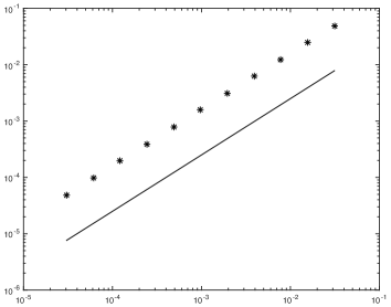
In fact, the order of convergence in (3.17) is sharp, as illustrated in Figure 1 for the choice $d=1$, $\lambda=-1$, $u^{0}=1$, $T=1$. Here, $r_{n}$ in computed for the uniform partition $\tau^{n}_{i}=\tau^{n}=2^{-n}$, $n=1,\dots,12$ or, equivalently, for $N^{n}=2^{n}$.

Figure 1. Values $r^{n}$ from (3.16) against $\tau^{n}$ (stars) with respect to order $1$ (solid) in log-log scale.

On a uniform partition of time step $\tau>0$, the solution of the new minimizing movement scheme $\{u_{i}\}$ and the solution $\{u_{i}^{e}\}$ of the Euler scheme read

$$u_{i}=\frac{u_{0}}{(1+\lambda\tau+\lambda^{2}\tau^{2})^{i}}\quad\text{and}\quad u_{i}^{e}=\frac{u_{0}}{(1+\lambda\tau)^{i}},$$ (3.18)

respectively. It is hence a standard matter to compute

$$|u_{i}-u^{e}_{i}|=|u_{0}|\left|\frac{(1+\lambda\tau)^{i}-(1+\lambda\tau+\lambda^{2}\tau^{2})^{i}}{(1+\lambda\tau+\lambda^{2}\tau^{2})^{i}(1+\lambda\tau)^{i}}\right|$$ (3.19)

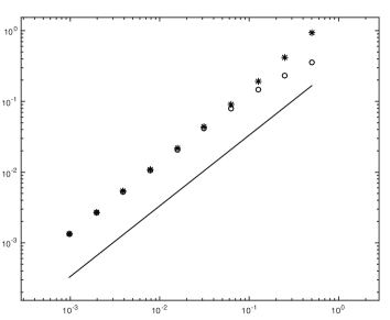
which scales like $\tau^{2}$ as $\tau\to 0$. As the Euler scheme is of first order, the same holds true for the new minimizing-movements scheme, see Figure 2 for $d=1$, $\lambda=-1$, $u_{0}=1$. Indeed, Figure 2 shows that this order is sharp. Note in fact that the new minimizing-movements scheme is proved in [24, Prop. 4.3] to be of first order for all nonnegative potentials $\phi$ in $C^{2}$ in finite dimensions.

Figure 2. $L^{\infty}$ error with respect to $\tau^{n}$ for the new minimizing-movements scheme (stars) and the Euler scheme (dots) in log-log scale. The solid line represents order $1$.

Assume now to be interested in computing the minimum of $\phi$ by following the discrete scheme for a fixed number $m$ of iterations, a classical strategy in optimization [10, 33]. In the specific case of our ODE example we compute from (3.18)

$$\phi(u_{m})=\frac{\lambda}{2(1+\lambda\tau+\lambda^{2}\tau^{2})^{2m}}\quad\text{and}\quad\phi(u_{m}^{e})=\frac{\lambda}{2(1+\lambda\tau)^{2m}}.$$ (3.20)

Due to the presence of the extra term $\lambda^{2}\tau^{2}$ in the denominator, the new scheme is advantageous with respect to Euler as for reduction of the potential after a fixed number of iterations. Note that this effect is enhanced by choosing large time steps.

Let us move to an infinite-dimensional example by considering the standard heat equation on the space time cylinder $\Omega\times(0,T)$ where $\Omega\subset\mathbb{R}^{d}$ is a smooth, open, and bounded set and homogeneous Dirichlet conditions are imposed (other choices being of course possible). We classically reformulate this as the gradient flow in $(L^{2}(\Omega),\|\cdot\|)$, of the Dirichlet energy

$$\phi(u)=\left\{\begin{array}[]{ll}\displaystyle\frac{1}{2}\int_{\Omega}|\nabla u(x)|^{2}\,{\rm d}x&\text{for}\ \ u\in H^{1}_{0}(\Omega)\\ \infty&\text{elsewhere in}\ L^{2}(\Omega).\end{array}\right.$$

where $\|\cdot\|$ is the norm corresponding to the natural $L^{2}$ scalar product $(\cdot,\cdot)$. In this case, we have that $\partial\phi(u)=-\Delta u$ with $D(\partial\phi)=H^{2}(\Omega)\cap H^{1}_{0}(\Omega)$. The symbol $\partial$ indicates the subdifferential in the sense of convex analysis [9]. In particular, $\partial\phi$ is single-valued and $|\partial\phi|(u)=\|\Delta u\|$ for all $u\in D(\partial\phi)$. The incremental functional $G:(0,\infty)\times H^{1}_{0}(\Omega)\times H^{2}(\Omega)\cap H^{1}_{0}(\Omega)$ hence reads

$$G(\tau,v,u)=\int_{\Omega}\left(\frac{1}{2}|\nabla u|^{2}+\frac{1}{2\tau}|u-v|^{2}+\frac{\tau}{2}|\Delta u|^{2}-\frac{1}{2}|\nabla v|^{2}\right){\rm d}x.$$

For all $v\in H^{1}_{0}(\Omega)$ given, the latter can be readily minimized in $H^{2}(\Omega)\cap H^{1}_{0}(\Omega)$. Given linearity one can easily identify the subgradient of $u\mapsto G(\tau,v,u)$ as

$$(\partial G(\tau,v,\cdot))(u)=-\Delta u+\frac{u-v}{\tau}+\tau\Delta^{2}u$$

and $D(\partial G(\tau,v,\cdot))=\{u\in H^{4}(\Omega)\cap H^{1}_{0}(\Omega)\,:\,\Delta u=0\ \text{on}\ \partial\Omega\}$. Hence, the minimizer $u$ of $G(\tau,v,\cdot)$ solves

$$u-\tau\Delta u+\tau^{2}\Delta^{2}u=v\ \ \text{a.e. in}\ \ \Omega,\quad u=\Delta u=0\ \ \text{on}\ \ \partial\Omega.$$ (3.21)

The latter is reminiscent of a singular perturbation of

$$u^{e}-\tau\Delta u^{e}=v\ \ \text{a.e. in}\ \ \Omega,\quad u^{e}=0\ \ \text{on}\ \ \partial\Omega,$$ (3.22)

corresponding instead to the incremental step of the Euler scheme.

Let now $\{w^{k}\}$ be a complete orthonormal basis of $L^{2}$ of eigenfunctions of $-\Delta$ with homogeneous Dirichlet boundary conditions, namely, $w^{k}\in H^{2}(\Omega)\cap H^{1}_{0}(\Omega)$ with $w^{k}\not=0$ and $-\Delta w^{k}=\lambda^{k}w^{k}$ for some $\lambda^{k}>0$. By inserting in (3.21)-(3.22) $u=\sum_{k}u^{k}w^{k}$, $u^{e}=\sum_{k}(u^{e})^{k}w^{k}$, and $v=\sum_{k}v^{k}w^{k}$ for $u^{k}:=(u,w^{k})$, $(u^{e})^{k}:=(u^{e},w^{k})$, and $v^{k}:=(v,w^{k})$, respectively, we get that

$$u^{k}=\frac{v^{k}}{1+\tau\lambda^{k}+(\tau\lambda^{k})^{2}}\quad\text{and}\quad(u^{e})^{k}=\frac{v^{k}}{1+\tau\lambda^{k}}.$$

In particular, by arguing as in (3.15) one readily checks that

$$\widehat{G}(\tau,v)=-\sum_{k}\frac{|v^{k}|^{2}(\lambda^{k})^{3}\tau^{2}}{2(1+\tau\lambda^{k}+(\tau\lambda^{k})^{2})}\leq 0$$

and condition (3.14) holds. By iterating on the time steps, the solution $\{u_{i}\}$ of the new minimizing movement scheme and that $\{u^{e}_{i}\}$ of the Euler scheme read $u_{i}=\sum_{k}u^{k}_{i}w^{k}$ and $u^{e}_{i}=\sum_{k}(u^{e})^{k}_{i}w^{k}$ where

$$u^{k}_{i}=\frac{(u^{0})^{k}}{(1+\tau\lambda^{k}+(\tau\lambda^{k})^{2})^{i}}\quad\text{and}\quad(u^{e}_{i})^{k}=\frac{(u^{0})^{k}}{(1+\tau\lambda^{k})^{i}}$$

and $(u^{0})^{k}:=(u^{0},w^{k})$. Proceeding as in (3.20) one computes

$$\phi(u_{m})=\frac{1}{2}\sum_{k}\lambda^{k}(u^{k}_{m})^{2}=\frac{1}{2}\sum_{k}\frac{\lambda^{k}((u^{0})^{k})^{2}}{(1+\tau\lambda^{k}+(\tau\lambda^{k}))^{2m}},$$

$$\phi(u_{m})=\frac{1}{2}\sum_{k}\lambda^{k}((u^{e}_{m})^{k}_{m})^{2}=\frac{1}{2}\sum_{k}\frac{\lambda^{k}((u^{0})^{k})^{2}}{(1+\tau\lambda^{k})^{2m}}$$

and the same observations as in the ODE case on the effectiveness of the reduction of the potential for a fixed number of iterations apply.

3.4. Literature

Before moving on, let us record here some other alternatives to the Euler scheme, specifically focusing on the case $p=2$.

Legendre and Turinici advance in [25] the midpoint scheme

$$u_{i}\in{\rm arg\,min}_{u}\Bigg{(}\inf\Bigg{(}2\phi(w)+\frac{1}{2\tau}d(u,u_{i-1})\ :\ w\in\Gamma(u,u_{i-1})\Bigg{)}\Bigg{)}$$

where

$$\Gamma(u,u_{i-1})=\{\gamma(1/2)\ :\ \gamma:[0,1]\to U\ \text{geodesic with}\ \gamma(0)=u_{i-1}\ \text{and}\ \gamma(1)=u\}.$$

By assuming (3.9)-(3.10), as well as some additional closure property relating to the specific structure of the set $\Gamma$, they prove that this midpoint scheme is solvable and convergent.

A variant of this scheme is also proposed in [25] in the specific case of nonbranching geodesic spaces, namely, spaces where any two points are connected by a unique geodesic. In these spaces, for all $w$ and $u_{i-1}$ there exists a unique $u$ such that $w\in\Gamma(u,u_{i-1})$. An extrapolated version of the Euler scheme is hence defined by the relations

$$u^{e}_{1/2}\in\Gamma(u_{i},u_{i-1})\ \ \text{where}\ \ u^{e}_{1/2}\in M_{E}(\tau/2,u_{i-1}).$$

Albeit not purely variational, this scheme is based on the solution of the Euler scheme with halved time step.

Matthes and Plazotta [26] address a variational version of the Backward Differentiation Formula (BDF2) method, namely,

$$u_{i}\in{\rm arg\,min}_{u\in D(\phi)}\left(\frac{1}{\tau}d^{2}(u,u_{i-1})-\frac{1}{4\tau}d^{2}(u,u_{i-2})+\phi(u)\right)\quad\text{for}\ i=2,\dots,N$$

where now both $u_{0}$ and $u_{1}$ are given. Under some lower semicontinuity and convexity conditions, it is proved in [26] that the scheme admits a solution, whose piecewise-in-time interpolant converges to a curve of maximal slope with rate $\tau^{1/2}$. It also shown that under natural regularity assumptions on the limiting time-continuous curve of maximal slope, the convergence rate can be $\tau$ at best.

Perturbations of the Euler method of the form

$$u_{i}\in{\rm arg\,min}_{u\in D(\phi)}\left(\frac{a_{i}^{\tau}}{2\tau}d^{2}(u,u_{i-1})+\phi(u)\right)\quad\text{for}\ i=2,\dots,N,$$

are considered by Tribuzio in [38]. Here, one is given the sequence of positive weights defined as $a_{i}^{\tau}=a^{\tau}(i\tau)$ for some functions $a^{\tau}:(0,\infty)\to(0,\infty)$. This generalization with respect to the classical Euler scheme yields a modification of the metric as time evolves. By asking $1/a^{\tau}$ to be locally equiintegrable with respect to $\tau$, one can prove that minimizers converge to curves of maximal slope according to a specific time-dependent limiting metric. Under some more general assumptions on $a^{\tau}$, discontinuous evolutions can also be obtained. These can be proved to be capable of exploring the different wells of a multiwell potential $\phi$.

Let us also mention the approach à la Crandall-Liggett by Clément and Desch [14, 15], see also [16], who recursively define $u^{n}_{0}=u^{0}$ and $u^{n}_{i}=J(u^{n}_{i-1})$ for $i=1,\dots,N=T/\tau$, where $J(u^{n}_{i-1})$ is the set of points $u\in D(\phi)$ fulfilling the inequality

$$\frac{1}{2\tau}d^{2}(u,w)-\frac{1}{2\tau}d^{2}(u_{i-1}^{n},w)+\frac{1}{2\tau}d^{2}(u,u_{i-1}^{n})+\phi(u)\leq\phi(w)\quad\forall w\in D(\phi).$$

Such points exist for $\phi$ geodesically convex and the corresponding interpolants $\overline{u}^{n}$ converge to evolutionary variational inequality solutions [28], a specific class of curves of maximal slope.

4. Conditional convergence

This section is devoted to the proof of Theorem 3.1. The ingredients of the argument are quite classical. Still, as already mentioned, the current minimizing-movement setting of (3.2) expedites the proof, for there is no need to resort to the De Giorgi variational interpolant [5, Def. 3.2.1].

Let $\{u_{0}^{n}\}$ be $d$-bounded with $u_{0}^{n}\stackrel{{\scriptstyle\sigma}}{{\to}}u^{0}$ and $\phi(u_{0}^{n})\to\phi(u^{0})$ fulfill (3.14). We have that

$$\phi(\overline{u}^{n}(t_{m}^{n}))+\frac{1}{p}\int_{0}^{t^{n}_{m}}|(\widehat{u}^{n})^{\prime}|^{p}(r)\,{\rm d}r+\frac{1}{q}\int_{0}^{t^{n}_{m}}|\partial\phi|^{q}(\overline{u}^{n}(r))\,{\rm d}r$$

$$\quad=\phi(u_{m}^{n})+\frac{1}{p}\sum_{i=1}^{m}(\tau_{i}^{n})^{1-p}d^{p}(u_{i-1}^{n},u_{i}^{n})+\frac{1}{q}\sum_{i=1}^{m}\tau_{i}^{n}|\partial\phi|^{q}(u_{i}^{n})$$

$$\quad=\sum_{i=1}^{m}G(\tau_{i}^{n},u_{i-1}^{n},u_{i}^{n})+\phi(u_{0}^{n}).$$ (4.23)

Condition (3.14) ensures that the above right-hand is bounded independently of $m=1,\dots,N^{n}$ and $n$. A first consequence of estimate (4.23) is that $\{u_{m}^{n}\}$ is $d$-bounded independently of $m=1,\dots,N^{n}$ and $n$. Indeed, one has that

$$d^{p}(u^{n}_{0},u^{n}_{m})\leq 2^{p-1}\sum_{i=1}^{m}d^{p}(u^{n}_{i-1},u^{n}_{i})\leq 2^{p-1}(\tau^{n})^{p-1}\sum_{i=1}^{m}(\tau_{i}^{n})^{1-p}d^{p}(u^{n}_{i-1},u^{n}_{i})$$

$$\leq\quad 2^{p-1}(\tau^{n})^{p-1}p\left(\sum_{i=1}^{m}G(\tau_{i}^{n},u_{i-1}^{n},u_{i}^{n})+\phi(u_{0}^{n})\right).$$

The right-hand side is bounded independently of $m=1,\dots,N^{n}$ and $n$. Since $\{u_{0}^{n}\}$ are $d$-bounded, the $d$-boundedness of $\{u_{m}^{n}\}$ follows.

As the sublevels of $\phi$ are sequentially $\sigma$-compact, one can apply the extended Ascoli-Arzelà Theorem from [5, Prop. 3.3.1] and find a not relabeled subsequence $\{\overline{u}^{n}\}$ such that $\overline{u}^{n}\stackrel{{\scriptstyle\sigma}}{{\to}}u$ pointwise, where $u:[0,T]\to U$, and $|(\widehat{u}^{n})^{\prime}|\to m$ weakly in $L^{p}(0,T)$. In particular, we have that $u(0)=\lim_{n\to\infty}u^{n}(0)=\lim_{n\to\infty}u^{n}_{0}=u^{0}$. For all $0<s\leq t<T$, define $s^{n}=\max\{t^{n}_{i}\,:\,t_{i}^{n}<s\}$ and $t^{n}=\min\{t^{n}_{i}\,:\,t<t^{n}_{i}\}$. Then,

$$d(u(s),u(t))\stackrel{{\scriptstyle\eqref{eq:compat}}}{{\leq}}\liminf_{n\to\infty}d(\overline{u}^{n}(s),\overline{u}^{n}(t))\leq\liminf_{n\to\infty}\int_{s^{n}}^{t^{n}}|(\widehat{u}^{n})^{\prime}|(r)\,{\rm d}r=\int_{s}^{t}m(r)\,{\rm d}r.$$

This entails that $u\in AC^{p}([0,T];U)$ since we just checked that the function $m\in L^{p}(0,T)$ fulfills (2.1). As $|u^{\prime}|$ is the minimal function in $L^{p}(0,T)$ fulfilling (2.1), we also have that $|u|\leq m$ almost everywhere and

$$\int_{0}^{t}|u^{\prime}|^{p}(r)\,{\rm d}r\leq\int_{0}^{t}m^{p}(r)\,{\rm d}r\leq\liminf_{\tau\to 0}\int_{0}^{t}|(\widehat{u}^{n})^{\prime}|^{p}(r)\,{\rm d}r\quad\forall t>0.$$

For all fixed $t\in(0,T]$, choose $t^{n}_{m}=t^{n}$ in (4.23) in order to get that

$$\phi(\overline{u}^{n}(t))+\frac{1}{p}\int_{0}^{\overline{t}^{n}(t)}|(\widehat{u}^{n})^{\prime}|^{p}(r)\,{\rm d}r+\frac{1}{q}\int_{0}^{\overline{t}^{n}(t)}|\partial\phi|^{q}(\overline{u}^{n}(r))\,{\rm d}r$$

$$\quad\stackrel{{\scriptstyle\eqref{eq:pass}}}{{\leq}}\sum_{i=1}^{N^{n}}(G(\tau_{i}^{n},u_{i-1}^{n},u_{i}^{n}))^{+}+\phi(u_{0}^{n}).$$

Owing to the sequential $\sigma$-lower semicontinuity of $\phi$ and $|\partial\phi|$, see (3.9)-(3.10), we can pass to the $\liminf$ in the latter and, using again condition (3.14) and the fact that $\phi(u^{n}_{0})\to\phi(u^{0})$, we obtain

$$\phi(u(t))+\frac{1}{p}\int_{0}^{t}|u^{\prime}|^{p}(r)\,{\rm d}r+\frac{1}{q}\int_{0}^{t}|\partial\phi|^{q}(u(r))\,{\rm d}r\leq\phi(u(0))\quad\forall t\in[0,T].$$ (4.24)

As $|\partial\phi|$ is a strong upper gradient for $\phi$ by (3.10), we have that

$$\phi(u(0))\leq\phi(u(t))+\int_{0}^{t}|\partial\phi|(u(r))\,|u^{\prime}|(r)\,{\rm d}r$$

$$\quad\leq\phi(u(t))+\frac{1}{p}\int_{0}^{t}|u^{\prime}|^{p}(r)\,{\rm d}r+\frac{1}{q}\int_{0}^{t}|\partial\phi|^{q}(u(r))\,{\rm d}r$$

so that (4.24) is actually an equality and $u$ is a curve of maximal slope in the sense of Definition 2.1.

5. Convergence in the geodesically convex case

We now turn to the proof of Theorem 3.2.

Recall that for all $\tau^{n}_{i}>0$ and $v\in D(\phi)$ the functional $u\in D(\phi)\mapsto E(\tau_{i}^{n},v,u)$ admits a minimizer. We first prove a $p$-variant for $p>1$ of the slope estimate [5, Lem. 3.1.3, p. 61], which was originally proved for $p=2$. In particular, we aim at the following

$$|\partial\phi|(u)\leq(\tau_{i}^{n})^{1-p}d^{p-1}(v,u)\quad\forall u\in M_{E}(\tau_{i}^{n},v).$$ (5.1)

Note that this estimate is already mentioned in [5, Rem. 3.1.7] without proof. We give an argument here. Let $w\in D(\phi)$ be given. From the minimality $E(\tau_{i}^{n},v,u)\leq E(\tau_{i}^{n},v,w)$ we deduce that

$$\phi(u)-\phi(w)\leq\frac{(\tau^{n}_{i})^{1-p}}{p}\Big{(}d^{p}(v,w)-d^{p}(v,u)\Big{)}$$

$$\quad\leq\frac{(\tau^{n}_{i})^{1-p}}{p}\Big{(}\big{(}d(u,w)+d(v,u)\big{)}^{p}-d^{p}(v,u)\Big{)}$$

$$\quad=\frac{(\tau^{n}_{i})^{1-p}}{p}\left(\sum_{k=0}^{\infty}\binom{p}{k}d^{k}(u,w)\,d^{p-k}(v,u)-d^{p}(v,u)\right)$$

$$\quad=d(u,w)\frac{(\tau^{n}_{i})^{1-p}}{p}\sum_{k=1}^{\infty}\binom{p}{k}d^{k-1}(u,w)\,d^{p-k}(v,u)$$

where we have made use of the generalized binomial formula and the generalized binomial coefficients

$$\binom{p}{k}=\frac{p(p-1)\dots(p-k+1)}{k!}.$$

Assume now that $w\not=u$, divide by $d(u,w)$, and compute the $\limsup$ as $w\to u$ in order to get

$$|\partial\phi|(u)=\limsup_{w\to u}\frac{\big{(}\phi(u)-\phi(w)\big{)}^{+}}{d(u,w)}\leq\limsup_{w\to u}\frac{(\tau^{n}_{i})^{1-p}}{p}\sum_{k=1}^{\infty}\binom{p}{k}d^{k-1}(u,w)\,d^{p-k}(v,u)$$

$$\quad=\frac{(\tau^{n}_{i})^{1-p}}{p}\binom{p}{1}d^{p-1}(v,u)={(\tau^{n}_{i})^{1-p}}d^{p-1}(v,u)$$

so that (5.1) holds. Above, we have used the fact that

$$0\leq\lim_{w\to u}\sum_{k=2}^{\infty}\binom{p}{k}d^{k-1}(u,w)\,d^{p-k}(v,u)\leq\lim_{w\to u}d(u,w)\sum_{k=2}^{\infty}\binom{p}{k}d^{p-k}(v,u)$$

$$\quad=\lim_{w\to u}d(u,w)\left((1+d(v,u))^{p}-\binom{p}{1}d^{p-1}(v,u)-\binom{p}{0}d^{p}(v,u)\right)=0.$$

Let now $u^{e}\in D(\phi)$ be a minimizer of $u\mapsto E(\tau_{i}^{n},u_{i-1}^{n},u)$. Taking into account the convexity assumption (3.12), let $\gamma:[0,1]\to U$ be a curve with $\gamma(0)=u_{i-1}^{n}$ and $\gamma(1)=u^{e}$, so that

$$E(\tau_{i}^{n},u_{i-1}^{n},u^{e})\leq E(\tau_{i}^{n},u_{i-1}^{n},\gamma(\theta))$$

$$\quad\stackrel{{\scriptstyle\eqref{eq:F2}}}{{\leq}}\theta E(\tau_{i}^{n},u_{i-1}^{n},u^{e})+(1-\theta)E(\tau_{i}^{n},u_{i-1}^{n},u_{i-1}^{n})$$

$$\quad-\theta(1-\theta)\frac{(p-1)(\tau_{i}^{n})^{1-p}+\lambda}{p}d^{p}(u_{i-1}^{n},u^{e})$$

where in the first inequality we have again used minimality. Let $\theta\in[0,1)$, divide by $1-\theta$, and take $\theta\to 1$ in order to get

$$E(\tau_{i}^{n},u_{i-1}^{n},u^{e})+\frac{(\tau_{i}^{n})^{1-p}}{q}d^{p}(u_{i-1}^{n},u^{e})$$

$$\quad\leq E(\tau_{i}^{n},u_{i-1}^{n},u_{i-1}^{n})-\frac{\lambda}{p}d^{p}(u_{i-1}^{n},u^{e}).$$ (5.2)

By taking the $q$-power of the slope estimate (5.1) with $v=u^{n}_{i-1}$ we get

$$|\partial\phi|^{q}(u^{e})\leq(\tau_{i}^{n})^{-p}d^{p}(u_{i-1}^{n},u^{e}).$$

We use this to estimate from below the second term on the left-hand side of (5.2) obtaining

$$E(\tau_{i}^{n},u_{i-1}^{n},u^{e})+\frac{\tau_{i}^{n}}{q}|\partial\phi|^{q}(u^{e})\leq E(\tau_{i}^{n},u_{i-1}^{n},u_{i-1}^{n})-\frac{\lambda}{p}d^{p}(u_{i-1}^{n},u^{e}).$$

As $E(\tau_{i}^{n},u_{i-1}^{n},u_{i-1}^{n})=0$, given any $u_{i}^{n}\in M_{G}(\tau_{i}^{n},u^{n}_{i-1})$ the latter entails that

$$G(\tau_{i}^{n},u_{i-1}^{n},u_{i}^{n})\leq G(\tau_{i}^{n},u_{i-1}^{n},u^{e})$$

$$\quad=E(\tau_{i}^{n},u_{i-1}^{n},u^{e})+\frac{\tau_{i}^{n}}{q}|\partial\phi|^{q}(u^{e})\leq-\frac{\lambda}{p}d^{p}(u_{i-1}^{n},u^{e}).$$ (5.3)

Recall now that the minimality $u^{e}\in M_{E}(\tau_{i}^{n},u^{n}_{i-1})$ and the nonnegativity of $\phi$ ensure that

$$\frac{(\tau_{i}^{n})^{1-p}}{p}d^{p}(u_{i-1}^{n},u^{e})\leq\phi(u_{i-1}^{n}).$$

Hence, inequality (5.3) yields

$$G(\tau_{i}^{n},u_{i-1}^{n},u_{i}^{n})\leq\lambda^{-}(\tau_{i}^{n})^{p-1}\phi(u_{i-1}^{n}).$$ (5.4)

Taking the sum on $i=1,\dots,m$ for $m\leq N^{n}$ we get

$$\phi(u_{m}^{n})+\frac{1}{p}\sum_{i=1}^{m}(\tau_{i}^{n})^{1-p}d^{p}(u_{i-1}^{n},u_{i}^{n})+\frac{1}{q}\sum_{i=1}^{m}\tau^{n}_{i}|\partial\phi|^{q}(u_{i}^{n})-\phi(u^{0})$$

$$\quad=\sum_{i=1}^{m}G(\tau^{n}_{i},u^{n}_{i-1},u^{n}_{i})\leq\lambda^{-}(\tau^{n})^{p-2}\sum_{i=0}^{m-1}\tau^{n}_{i}\phi(u_{i}^{n}).$$

We can hence use the discrete Gronwall Lemma and deduce that

$$\phi(u_{m}^{n})+\frac{1}{p}\sum_{i=1}^{m}(\tau_{i}^{n})^{1-p}d^{p}(u_{i-1}^{n},u_{i}^{n})+\frac{1}{q}\sum_{i=1}^{m}\tau^{n}_{i}|\partial\phi|^{q}(u_{i}^{n})$$

$$\quad\leq\phi(u^{0})\,{\rm exp}\left(\lambda^{-}(\tau^{n})^{p-2}t^{n}_{m}\right).$$

Going back to (5.4), this entails that

$$(G(\tau_{i}^{n},u_{i-1}^{n},u_{i}^{n}))^{+}\leq\lambda^{-}(\tau_{i}^{n})^{p-1}\phi(u^{0})\,{\rm exp}\left(\lambda^{-}(\tau^{n})^{p-2}T\right).$$

Adding up for $i=1,\dots,N^{n}$ we get

$$\sum_{i=1}^{N^{n}}\big{(}G(\tau_{i}^{n},u_{i-1}^{n},u_{i}^{n})\big{)}^{+}\leq\lambda^{-}(\tau^{n})^{p-2}T\,\phi(u^{0})\,{\rm exp}\left(\lambda^{-}(\tau^{n})^{p-2}T\right)=:R^{n}.$$

If $\lambda\geq 0$, we have that $R^{n}=0$ and condition (3.14) trivially holds. If $\lambda<0$ and $p>2$, one can readily check that $R^{n}\to 0$ as $n\to\infty$ and (3.14) again holds.

6. Convergence without geodesic convexity

We now turn to the proof of Theorem 3.3, where the convexity assumption is replaced by the generalized one-sided Taylor-expansion assumption (3.13). The argument follows the general strategy of [5, Chap. 3], by revisiting the theory and adapting it to the incremental functional $G$ and to the case $p>1$. In particular, it is fairly different with respect to that of Section 5 and does not rely on the existence of solutions of the Euler scheme. We prepare some preliminary arguments in Subsections 6.1-6.4, deduce an a priori estimate in Subsection 6.5 and eventually present the proof of Theorem 3.3 in Subsection 6.6.

6.1. A measurable selection in $\tau\mapsto M_{G}(\tau,v)$

Let us recall that for all $\tau\in(0,\tau_{*}]$ and $v\in D(\phi)$ the set of minimizers $M_{G}(\tau,v)$ is not empty. By additionally defining $M_{G}(0,v)=\{v\}$, the set-valued function $\tau\in[0,\tau_{*}]\mapsto M_{G}(\tau,v)$ has nonempty values. The aim of this section is to check that it admits a measurable selection, namely,

$$\exists\,\tau\in[0,\tau_{*}]\mapsto u_{\tau}\in M_{G}(\tau,v)\ \ \text{measurable}.$$ (6.1)

To this aim, we firstly check that $M_{G}(\tau,v)$ is closed for all $\tau\in[0,\tau_{*}]$. Indeed, assume $\tau>0$ (the case $\tau=0$ being trivial) and let $u_{k}\in M_{G}(\tau,v)$ with $u_{k}\to u_{\infty}$. In particular, we have that

$$\phi(u_{k})+\frac{\tau^{1-p}}{p}d^{p}(v,u_{k})+\frac{\tau}{q}|\partial\phi|^{q}(u_{k})-\phi(v)=G(\tau,v,u_{k})\leq G(\tau,v,w)$$

for any $w\in D(|\partial\phi|).$ Owing to the lower semicontinuity (3.9)-(3.10) we can pass to the lower limit and check that $G(\tau,v,u_{\infty})\leq G(\tau,v,w)$, so that $u_{\infty}\in M_{G}(\tau,v)$ as well.

Secondly, we check that $\tau\mapsto M_{G}(\tau,v)$ is measurable in the sense of set-valued functions [39]. In particular, we have to check that, for all $C\subset U$ closed, the set

$$A=\{\tau\in[0,\tau_{*}]\ :\ M_{G}(\tau,v)\cap C\not=\emptyset\}$$

is measurable. Indeed, one can prove that $A$ is closed: Take $\tau_{k}\in A$ such that $\tau_{k}\to\tau_{\infty}$ and let $u_{k}\in M_{G}(\tau_{k},v)\cap C$. We have that

$$\phi(u_{k})+\frac{\tau^{1-p}_{k}}{p}d^{p}(v,u_{k})+\frac{\tau_{k}}{q}|\partial\phi|^{q}(u_{k})-\phi(v)=G(\tau_{k},v,u_{k})$$

$$\quad\leq G(\tau_{k},v,v)=\frac{\tau_{k}}{q}|\partial\phi|^{q}(v)<\infty.$$ (6.2)

One can hence deduce uniform estimates for $u_{k}$ and from compactness (3.9) one extracts a not relabeled subsequence such that $u_{k}\to u_{\infty}$. If $\tau_{\infty}>0$, by passing to the liminf in the minimality condition for $u_{k}$ one gets

$$G(\tau_{\infty},v,u_{\infty})\leq\liminf_{k\to\infty}G(\tau_{k},v,u_{k})\leq\liminf_{k\to\infty}G(\tau_{k},v,w)=G(\tau_{\infty},v,w)$$

for any $w\in D(|\partial\phi|)$. This implies that $u_{\infty}\in M_{G}(\tau_{\infty},v)$. On the other hand, if $\tau_{\infty}=0$ we obtain from (6.2) that

$$d^{p}(v,u_{k})\leq p\tau_{k}^{p-1}\phi(v)+\frac{p\tau_{k}^{p}}{q}|\partial\phi|^{q}(v)\to 0,$$

so that $u_{\infty}=v\in M_{G}(0,v)$. Since $C$ is closed, $u_{\infty}\in C$ as well and we have proved that $M_{G}(\tau_{\infty},v)\cap C$ is not empty. In particular, $\tau_{\infty}\in A$ which is hence closed.

As the metric space $(U,d)$ is complete and separable and $\tau\mapsto M_{G}(\tau,v)$ has nonempty and closed values, the Ryll-Nardzewski Theorem [36] applies and (6.1) holds.

6.2. Continuity of $\tau\mapsto\widehat{G}(\tau,v)$

We now turn our attention to the real map $\tau\in[0,\tau_{*}]\mapsto\widehat{G}(\tau,v)$ for some given $v\in D(\phi)$, where we define $\widehat{G}(0,v)=0$. In order to check that this function is continuous on $[0,\tau_{*}]$, take $\tau_{k}\in[0,\tau_{*}]\to\tau_{\infty}$ and $u_{k}\in M_{G}(\tau_{k},v)$. Following the argument of Subsection 6.1, we can extract a not relabeled subsequence such that $u_{k}\to u_{\infty}\in M_{G}(\tau_{\infty},v)$.

If $\tau_{\infty}>0$ the lower semicontinuity (3.9)-(3.10) implies that

$$G(\tau_{\infty},v,u_{\infty})\leq\liminf_{k\to\infty}G(\tau_{k},v,u_{k})\leq\limsup_{k\to\infty}G(\tau_{k},v,u_{k})$$

$$\quad\leq\limsup_{k\to\infty}G(\tau_{k},v,u_{\infty})=G(\tau_{\infty},v,u_{\infty}).$$

The case $\tau_{\infty}=0$ is even simpler as $u_{\infty}=v$ and we can compute

$$0=\widehat{G}(0,v)=\phi(u_{\infty})-\phi(v)\leq\liminf_{k\to\infty}\phi(u_{k})-\phi(v)\leq\liminf_{k\to\infty}G(\tau_{k},v,u_{k})$$

$$\quad\leq\limsup_{k\to\infty}G(\tau_{k},v,u_{k})\leq\limsup_{k\to\infty}G(\tau_{k},v,v)=\lim_{k\to\infty}\frac{\tau_{k}}{q}|\partial\phi|^{q}(v)=0.$$ (6.3)

In both cases, we have proved that $\widehat{G}(\tau_{k},v)\to\widehat{G}(\tau_{\infty},v)$.

6.3. Differentiability of $\tau\mapsto\widehat{G}(\tau,v)$

The aim of the subsection is to show that $\tau\mapsto\widehat{G}(\tau,v)$ is even locally Lipschitz continuous and to compute its almost-everywhere derivative, see equation (6.6) below.

Take $0<\tau_{0}<\tau_{1}<\tau_{*}$, $u_{0}\in M_{G}(\tau_{0},v)$, and $u_{1}\in M_{G}(\tau_{1},v)$ where $v\in D(\phi)$ is fixed. From minimality we deduce

$$\widehat{G}(\tau_{1},v)\leq G(\tau_{1},v,u_{0})=\widehat{G}(\tau_{0},v)+\frac{\tau_{1}^{1-p}-\tau_{0}^{1-p}}{p}d^{p}(v,u_{0})+\frac{\tau_{1}-\tau_{0}}{q}|\partial\phi|^{q}(u_{0})$$

so that one has

$$\widehat{G}(\tau_{1},v)-\widehat{G}(\tau_{0},v)\leq\frac{\tau_{1}^{1-p}-\tau_{0}^{1-p}}{p}d^{p}(v,u_{0})+\frac{\tau_{1}-\tau_{0}}{q}|\partial\phi|^{q}(u_{0}).$$

By exchanging the roles of $\tau_{0}$ and $\tau_{1}$ we also get

$$\widehat{G}(\tau_{0},v)-\widehat{G}(\tau_{1},v)\leq\frac{\tau_{0}^{1-p}-\tau_{1}^{1-p}}{p}d^{p}(v,u_{1})+\frac{\tau_{0}-\tau_{1}}{q}|\partial\phi|^{q}(u_{1}).$$

By dividing by $\tau_{1}-\tau_{0}$ we hence obtain

$$\frac{\tau_{1}^{1-p}-\tau_{0}^{1-p}}{p(\tau_{1}-\tau_{0})}d^{p}(v,u_{1})\leq\frac{\tau_{1}^{1-p}-\tau_{0}^{1-p}}{p(\tau_{1}-\tau_{0})}d^{p}(v,u_{1})+\frac{1}{q}|\partial\phi|^{q}(u_{1})$$

$$\quad\leq\frac{\widehat{G}(\tau_{1},v)-\widehat{G}(\tau_{0},v)}{\tau_{1}-\tau_{0}}$$

$$\quad\leq\frac{\tau_{1}^{1-p}-\tau_{0}^{1-p}}{p(\tau_{1}-\tau_{0})}d^{p}(v,u_{0})+\frac{1}{q}|\partial\phi|^{q}(u_{0})\leq\frac{1}{q}|\partial\phi|^{q}(u_{0}).$$ (6.4)

The latter implies that $\tau\mapsto\widehat{G}(\tau,v)$ is locally Lipschitz continuous on $(0,\tau_{*}]$. Indeed, take $0<\underline{\tau}<\tau_{*}$ and $\tau\in[\underline{\tau},\tau_{*}]$. Given $u_{\tau}\in M_{G}(\tau,v)$, we readily deduce that

$$d^{p}(v,u_{\tau})\leq p\tau^{p-1}_{*}\phi(v)+\frac{p\tau^{p}_{*}}{q}|\partial\phi|^{q}(v),$$

$$\frac{1}{q}|\partial\phi|^{q}(u_{\tau})\leq\frac{1}{\underline{\tau}}\phi(v)+\frac{1}{q}|\partial\phi|^{q}(v),$$

$${}-\frac{\tau_{1}^{1-p}-\tau_{0}^{1-p}}{p(\tau_{1}-\tau_{0})}\leq\frac{1}{q\tau_{0}^{p}}\leq\frac{1}{q\underline{\tau}^{p}}.$$

In particular, moving from (6.4), for all $\underline{\tau}\in(0,\tau_{*}]$ we find $C_{\underline{\tau}}$ depending on $\underline{\tau}$, $\phi(v)$, and $|\partial\phi|(v)$ such that

$$\left|\frac{\widehat{G}(\tau_{1},v)-\widehat{G}(\tau_{0},v)}{\tau_{1}-\tau_{0}}\right|\leq C_{\underline{\tau}}\quad\forall\underline{\tau}<\tau_{0}<\tau_{1}<\tau_{*}.$$

Hence, $\tau\in(0,\tau_{*}]\mapsto\widehat{G}(\tau,v)$ is locally Lipschitz continuous and therefore almost everywhere differentiable in $(0,\tau_{*})$.

Define now

$$\overline{f}(\tau_{0},\tau_{1})=\sup\left\{\frac{\tau_{1}^{1-p}-\tau_{0}^{1-p}}{p(\tau_{1}-\tau_{0})}d^{p}(v,u_{1})+\frac{1}{q}|\partial\phi|^{q}(u_{1})\ :\ u_{1}\in M_{G}(\tau_{1},v)\right\},$$

$$\underline{f}(\tau_{0},\tau_{1})=\inf\left\{\frac{\tau_{1}^{1-p}-\tau_{0}^{1-p}}{p(\tau_{1}-\tau_{0})}d^{p}(v,u_{0})+\frac{1}{q}|\partial\phi|^{q}(u_{0})\ :\ u_{0}\in M_{G}(\tau_{0},v)\right\}.$$

By using again relation (6.4) one has

$$\overline{f}(\tau_{0},\tau_{1})\leq\frac{\widehat{G}(\tau_{1},v)-\widehat{G}(\tau_{0},v)}{\tau_{1}-\tau_{0}}\leq\underline{f}(\tau_{0},\tau_{1}).$$ (6.5)

Let $\tau\in(0,\tau_{*})$ be such that $\tau\mapsto\widehat{G}(\tau,v)$ is differentiable at $\tau$, take $h\in(0,\tau_{*}-\tau)$ and any $u_{\tau+h}\in M_{G}(\tau+h,v)$. By arguing as in Subsection 6.1, one can extract a not relabeled subsequence $u_{\tau+h}\to u_{\tau}$ as $h\to 0$ and check that $u_{\tau}\in M_{G}(\tau,v)$. Moreover, going back to (6.5) and choosing $\tau_{0}=\tau$ and $\tau_{1}=\tau+h$ we deduce that

$$-\frac{\tau^{-p}}{q}d^{p}(v,u_{\tau})+\frac{1}{q}|\partial\phi|^{q}(u_{\tau})\leq\liminf_{h\to 0}\overline{f}(\tau,\tau+h)$$

$$\quad=\frac{\rm d}{{\rm d}\tau}\widehat{G}(\tau,v)\leq\liminf_{h\to 0}\underline{f}(\tau,\tau+h)\leq-\frac{\tau^{-p}}{q}d^{p}(v,\tilde{u}_{\tau})+\frac{1}{q}|\partial\phi|^{q}(\tilde{u}_{\tau})$$

where $\tilde{u}_{\tau}$ is any element of $M_{G}(\tau,v)$. Passing to the infimum in $M_{G}(\tau,v)$ left and right we get

$$\frac{\rm d}{{\rm d}\tau}\widehat{G}(\tau,v)=\inf\left\{-\frac{\tau^{-p}}{q}d^{p}(v,u_{\tau})+\frac{1}{q}|\partial\phi|^{q}(u_{\tau})\ :\ u_{\tau}\in M_{G}(\tau,v)\right\}$$ (6.6)

almost everywhere in $(0,\tau_{*})$.

6.4. Slope estimate

Let us prepare a version of the slope estimate (5.1) adapted to our setting, namely for points in $u\in M_{G}(\tau,v)$ for $v\in D(\phi)$ instead of $M_{E}(\tau,v)$. Let $w\in D(|\partial\phi|)$ be given. From minimality we deduce that

$$\phi(u)-\phi(w)+\frac{\tau}{q}|\partial\phi|^{q}(u)-\frac{\tau}{q}|\partial\phi|^{q}(w)\leq\frac{\tau^{1-p}}{p}\left(d^{p}(v,w)-d^{p}(v,u)\right)$$

$$\leq d(u,w)\frac{\tau^{1-p}}{p}\sum_{k=1}^{\infty}\binom{p}{k}d^{k-1}(u,w)d^{p-k}(v,u).$$

By assuming that $w\not=u$, dividing by $d(u,w)$, and taking $w\to u$ we get

$$|\partial(\phi+\tau|\partial\phi|^{q}/q)|(u)\leq\tau^{1-p}d^{p-1}(v,u)\quad\forall u\in M_{G}(\tau,v).$$ (6.7)

This proves in particular the additional regularity

$$M_{G}(\tau,v)\subset D(\partial(\phi+\tau|\partial\phi|^{q}/q))$$

for minimizers of $G$.

6.5. A priori estimate

Let now $\{u_{i}^{n}\}_{i=0}^{N^{n}}$ solve the incremental minimization problem (3.2) with $u^{0}$ replaced by the approximating $u^{0n}\in M_{E}(\tau^{n},u^{0})$. From minimality we obtain that

$$\phi(u^{n}_{i})+\frac{\tau^{n}_{i}}{q}|\partial\phi|^{q}(u^{n}_{i})+\frac{1}{p}(\tau^{n}_{i})^{1-p}d^{p}(u^{n}_{i-1},u^{n}_{i})\leq\phi(u^{n}_{i-1})+\frac{\tau^{n}_{i}}{q}|\partial\phi|^{q}(u^{n}_{i-1}).$$ (6.8)

Taking into account the one-sided nondegeneracy of the time partition

$$(\tau^{n}_{i}-\tau^{n}_{i-1})^{+}/\tau^{n}_{i-1}\leq C\tau^{n}$$

we can control the above right-hand side of (6.8) as follows

$$\phi(u^{n}_{i-1})+\frac{\tau^{n}_{i}}{q}|\partial\phi|^{q}(u^{n}_{i-1})=\phi(u^{n}_{i-1})+\frac{\tau^{n}_{i-1}}{q}|\partial\phi|^{q}(u^{n}_{i-1})+\frac{\tau_{i}^{n}-\tau^{n}_{i-1}}{q}|\partial\phi|^{q}(u^{n}_{i-1})$$

$$\quad\leq\phi(u^{n}_{i-1})+\frac{\tau^{n}_{i-1}}{q}|\partial\phi|^{q}(u^{n}_{i-1})+C\tau^{n}\frac{\tau^{n}_{i-1}}{q}|\partial\phi|^{q}(u^{n}_{i-1}).$$

Owing to this bound, we can take the sum in (6.8) for $i=2,\dots,m$ and get

$$\phi(u_{m}^{n})+\frac{\tau^{n}_{m}}{q}|\partial\phi|^{q}(u^{n}_{m})+\frac{1}{p}\sum_{i=1}^{m}(\tau^{n}_{i})^{1-p}d^{p}(u_{i-1}^{n},u_{i}^{n})$$

$$\quad\leq\phi(u^{n}_{1})+\frac{\tau^{n}_{1}}{q}|\partial\phi|^{q}(u^{n}_{1})+C\sum_{i=2}^{m}\tau^{n}\frac{\tau^{n}_{i-1}}{q}|\partial\phi|^{q}(u^{n}_{i-1})$$

$$\quad\stackrel{{\scriptstyle\eqref{eq:3}}}{{\leq}}\phi(u^{0n})+\frac{\tau^{n}}{q}|\partial\phi|^{q}(u^{0n})+C\sum_{j=1}^{m-1}\tau^{n}\frac{\tau^{n}_{j}}{q}|\partial\phi|^{q}(u^{n}_{j}).$$

By applying the discrete Gronwall Lemma we hence obtain

$$\phi(u_{m}^{n})+\frac{\tau^{n}_{m}}{q}|\partial\phi|^{q}(u^{n}_{m})+\frac{1}{p}\sum_{i=1}^{m}(\tau^{n}_{i})^{1-p}d^{p}(u_{i-1}^{n},u_{i}^{n})$$

$$\quad\leq C\left(\phi(u^{0n})+\frac{\tau^{n}}{q}|\partial\phi|^{q}(u^{0n})\right).$$ (6.9)

Recall now that $u^{0n}\in M_{E}(\tau^{n},u^{0})$ and use the slope estimate (5.1) to get that

$$\frac{\tau^{n}}{q}|\partial\phi|^{q}(u^{0n})\leq\frac{1}{q}(\tau^{n})^{1-p}d^{p}(u^{0},u^{0n})\leq\frac{p}{q}\phi(u^{0}).$$

Hence, $\{u^{0n}\}$ are in particular $d$-bounded and the bound (6.9) entails the estimate

$$\phi(u_{m}^{n})+\frac{\tau^{n}_{m}}{q}|\partial\phi|^{q}(u^{n}_{m})+\frac{1}{p}\sum_{i=1}^{m}\tau^{1-p}d^{p}(u_{i-1}^{n},u_{i}^{n})\leq C\left(1+\frac{p}{q}\right)\phi(u^{0})$$

$$\quad\forall m=1,\dots,N^{n},\ \forall n.$$ (6.10)

6.6. Conclusion of the proof

For all $i=1,\dots,N^{n}$ and $\tau_{0}\in(0,\tau^{n}_{i}]$ we use the Lipschitz continuity of $\tau\in(0,\tau^{n}_{i}]\mapsto\widehat{G}(\tau,u^{n}_{i-1})$ and write

$$\widehat{G}(\tau_{i}^{n},u_{i-1}^{n})=\widehat{G}(\tau_{0},u_{i-1}^{n})+\int_{\tau_{0}}^{\tau_{i}^{n}}\frac{\rm d}{\rm d\tau}\widehat{G}(\tau,u^{n}_{i-1})\,{\rm d}\tau.$$ (6.11)

Let now $\tau\in[\tau_{0},\tau^{n}_{i}]\mapsto u_{\tau}$ be a measurable selection in $M_{G}(\tau,u^{n}_{i-1})$. The existence of such a selection is ascertained in Subsection 6.1. Take $\tau_{0}\to 0$ in (6.11), use $\widehat{G}(\tau_{0},u^{n}_{i-1})\to 0$ from (6.3) and (6.6) to get

$$G(\tau^{n}_{i},u^{n}_{i-1},u^{n}_{i})\leq\int_{0}^{\tau^{n}_{i}}\left(-\frac{\tau^{-p}}{q}d^{p}(u^{n}_{i-1},u_{\tau})+\frac{1}{q}|\partial\phi|^{q}(u_{\tau})\right){\rm d}\tau.$$ (6.12)

In order to conclude the proof of Theorem 3.2, one has to check that condition (3.14) holds, so that Theorem 3.1 applies. This calls for controlling the right-hand side of (6.12). By means of the slope estimate (6.7) for $v=u^{n}_{i-1}$ and $u=u_{\tau}$ we can control the right-hand of (6.12) as

$$G(\tau^{n}_{i},u^{n}_{i-1},u^{n}_{i})\leq\int_{0}^{\tau^{n}_{i}}\left(\frac{1}{q}|\partial\phi|^{q}(u_{\tau})-\frac{1}{q}|\partial(\phi+\tau|\partial\phi|^{q}/q)|^{q}(u_{\tau})\right){\rm d}\tau.$$

We now use estimate (6.10) and the generalized one-sided Taylor expansion condition (3.13) in order to conclude that

$$\sum_{i=1}^{N^{n}}\left(G(\tau^{n}_{i},u^{n}_{i-1},u^{n}_{i})\right)^{+}\leq\frac{1}{q}\sum_{i=1}^{N^{n}}\int_{0}^{\tau^{n}_{i}}g(\tau)\,{\rm d}\tau$$

$$\quad=\frac{1}{q}\sum_{i=1}^{N^{n}}\tau^{n}_{i}\left(\frac{1}{\tau^{n}_{i}}\int_{0}^{\tau^{n}_{i}}g(\tau)\,{\rm d}\tau\right)\leq\frac{T}{q}\frac{1}{\tau^{n}}\int_{0}^{\tau^{n}}g(\tau)\,{\rm d}\tau.$$

As $(1/\tau^{n})\int_{0}^{r}g(\tau^{n})\,{\rm d}\tau\searrow 0$ as $\tau^{n}\to 0$ condition (3.14) holds. The statement hence follows from Theorem 3.1.

7. Applications in linear spaces

We collect in this section some comments on the application of the abstract convergence results of Theorem 3.1-3.3 in linear finite and infinite-dimensional spaces.

Let us start from the convex case of Theorem 3.2. We hence restrict to $p=2$, for assumption (3.12) cannot hold for $p\not=2$ in linear spaces, as commented in Subsection 3.1. Correspondingly, the potential $\phi$ is requires to be convex ($\lambda\geq 0$).

In the finite-dimensional ODE case, let the proper, convex potential $\phi:\mathbb{R}^{d}\to[0,\infty]$ and the initial datum $u^{0}\in D(\phi)$ be given. In this case, we have that $|\partial\phi|(u)=|(\partial\phi(u))^{\circ}|$, where $(\partial\phi(u))^{\circ}$ is the element of minimal norm in the convex and closed set $\partial\phi(u)$. In particular, $|\partial\phi|(u)$ is lower semicontinuous. As such, the new minimizing-movements scheme (3.2) has a solution $\{u_{i}^{n}\}$ for any partition and the corresponding interpolants converge to a solution of $u^{\prime}+\partial\phi(u)\ni 0$, up to subsequences.

In order to give an application of Theorem 3.2 in infinite dimensions, we consider

$$\partial_{t}u-\nabla{\cdot}\beta(\nabla u)+\alpha(u)\ni 0\quad\text{in}\ \ \Omega\times(0,T).$$ (7.13)

Here, $\Omega\subset\mathbb{R}^{d}$ is open, bounded, and smooth, $u:\Omega\times(0,T)\to\mathbb{R}$ is scalar-valued, and $\partial_{t}$ and $\nabla$ indicate partial derivatives in time and space, respectively. We assume that $\beta=\partial\widehat{\beta}$ and $\alpha=\partial\alpha$ where the potentials $\widehat{\beta}:\mathbb{R}^{d}\to[0,\infty]$ and $\widehat{\alpha}:\mathbb{R}\to[0,\infty]$ are proper and convex. In addition, we assume $\widehat{\beta}$ to be coercive in the following sense

$$\exists\,c_{\beta}>0,\ m>\frac{2d}{d+2}:\quad\widehat{\beta}(\xi)\geq c_{\beta}|\xi|^{m}-\frac{1}{c_{\beta}}\quad\forall\xi\in\mathbb{R}^{d}.$$ (7.14)

Equation (7.13) is intended to be complemented with homogeneous Dirichlet boundary conditions (other choices being of course possible) hence corresponding to the gradient flow in $U=L^{2}(\Omega)$ of the functional

$$\phi(u)=\left\{\begin{array}[]{ll}\displaystyle\int_{\Omega}\big{(}\widehat{\beta}(\nabla u)+\widehat{\alpha}(u)\big{)}\,{\rm d}x&\text{for}\ \ u\in W^{1,m}_{0}(\Omega),\\ &\quad\text{with}\ \widehat{\beta}(\nabla u)+\widehat{\alpha}(u)\in L^{1}(\Omega)\\[5.69054pt] \infty&\text{elsewhere in}\ \ L^{2}(\Omega).\end{array}\right.$$ (7.15)

As $\phi:U\to[0,\infty]$ is convex, proper, and lower semicontinuous, we have that $u\mapsto\partial\phi(u)$ is strongly-weakly closed and $|\partial\phi|(u)=\|(\partial\phi(u))^{\circ}\|$ (norm in $L^{2}(\Omega)$) is lower semicontinuous. Moreover, $\partial\phi$ fulfills the chain rule [9, Lem. 3.3], so that $|\partial\phi|$ is a strong upper gradient. Note that the sublevels of $\phi$ are bounded in $W^{1,m}_{0}(\Omega)$, which embeds compactly into $L^{2}(\Omega)$. We can hence apply Theorem 3.2. In particular, the new minimizing-movements scheme (3.2) has a solution, which converges to a solution of (7.13), up to subsequences.

Let us now turn to some application of Theorem 3.3 to nonconvex problems. In the finite-dimensional case, assume $\phi$ to be twice differentiable and coercive with $\nabla\phi$ and ${\rm D}^{2}\phi$ locally bounded. Then, one computes

$$|\nabla\phi(u)|^{q}-|\nabla(\phi(u)+\tau|\nabla\phi(u)|^{q}/q)|^{q}$$

$$\quad=|\nabla\phi(u)|^{q}-|\nabla\phi(u)+\tau|\nabla\phi(u)|^{q-2}{\rm D}^{2}\phi(u)\,\nabla\phi(u)|^{q}$$

$$\quad\leq\left(\big{|}\nabla\phi(u)+\tau|\nabla\phi(u)|^{q-2}{\rm D}^{2}\phi(u)\,\nabla\phi(u)\big{|}+\big{|}\tau|\nabla\phi(u)|^{q-2}{\rm D}^{2}\phi(u)\,\nabla\phi(u)\big{|}\right)^{q}$$

$$\qquad-\big{|}\nabla\phi(u)+\tau|\nabla\phi(u)|^{q-2}{\rm D}^{2}\phi(u)\,\nabla\phi(u)\big{|}^{q}$$

$$\quad\leq\tau\sum_{k=1}^{\infty}\binom{q}{k}\big{|}\nabla\phi(u)+\tau|\nabla\phi(u)|^{q-2}{\rm D}^{2}\phi(u)\,\nabla\phi(u)\big{|}^{q-k}\big{|}\nabla\phi(u)|^{q-2}{\rm D}^{2}\phi(u)\,\nabla\phi(u)\big{|}^{k}$$

$$\quad\leq\tau\left(\big{|}\nabla\phi(u)+\tau|\nabla\phi(u)|^{q-2}{\rm D}^{2}\phi(u)\,\nabla\phi(u)\big{|}+\big{|}|\nabla\phi(u)|^{q-2}{\rm D}^{2}\phi(u)\,\nabla\phi(u)\big{|}\right)^{q}.$$

Hence, the one-sided Taylor-expansion condition (3.13) holds for the choice

$$g(\tau)=\tau\sup_{\phi(v)\leq C}\left(|\nabla\phi(v)|+2|\nabla\phi(v)|^{q-1}|{\rm D}^{2}\phi(v)|\right)^{q}.$$

Note that the above computation simplifies in case $p=2$, for we have

$$|\nabla\phi(u)|^{2}-|\nabla(\phi(u)+\tau|\nabla\phi(u)|^{2}/2)|^{2}=|\nabla\phi(u)|^{2}-|\nabla\phi(u)+\tau{\rm D}^{2}\phi(u)\,\nabla\phi(u)|^{2}$$

$$\quad-\tau^{2}|{\rm D}^{2}\phi(u)\,\nabla\phi(u)|^{2}-2\tau\nabla\phi(u){\cdot}({\rm D}^{2}\phi(u)\,\nabla\phi(u)).$$

In particular, if $\phi$ is convex condition (3.13) holds with the trivial choice $g(\tau)=0$. In all cases, if ${\rm D}^{2}\phi(u)$ is bounded below on sublevels of $\phi$ in the following sense

$$\forall C>0,\,\exists c>0,\,\forall v,\,\xi\in\mathbb{R}^{d}\ \text{with}\ \phi(v)\leq C:\quad\xi{\cdot}{\rm D}^{2}\phi(v)\xi\geq-\frac{c}{2}|\xi|^{2}$$ (7.16)

and $\nabla\phi(u)$ is bounded on the sublevels of $\phi$, namely, $|\nabla\phi(u)|\leq\ell(\phi(u))$ for some $\ell$ increasing, we can choose $g(\tau)=2\tau c(\ell(C))^{2}$ in order to get again condition (3.13). This in particular applies to $\phi\in C^{2}$ and coercive. In all cases, we can apply Theorem 3.3 and deduce that the solution of the new minimizing-movements scheme converges up to subsequences to a solution of (1.3).

Let us now turn to the infinite-dimensional case. To simplify notation, let again $p=2$ and $U=L^{2}(\Omega)$ (the case $p\not=2$ and $U=L^{p}(\Omega)$ can also be treated) and define $\phi$ as in (7.15) by dropping the convexity requirement on $\widehat{\alpha}$. More precisely, we ask $\beta={\rm D}\widehat{\beta}\in C^{2}(\mathbb{R}^{d};\mathbb{R}^{d})$ and $\alpha=\widehat{\alpha}^{\prime}\in C^{2}(\mathbb{R})$ and $\widehat{\beta}$ fulfill the coercivity (7.14). In this case, we have that

$$\partial\phi(u)=-\nabla{\cdot}\beta(\nabla u)+\alpha(u),$$

$$\quad\text{with}\ \ D(\partial\phi)=\{u\in L^{2}(\Omega)\ :\ -\nabla{\cdot}\beta(\nabla u)+\alpha(u)\in L^{2}(\Omega)\}.$$

Recall that the Fréchet subdifferential [33] of $\psi:U\to[0,\infty]$ at $u\in D(\psi)$ is the set

$$\partial\psi(u)=\left\{\xi\in U\ :\ \liminf_{v\to u}\frac{\psi(v)-\psi(u)-(\xi,v-u)}{\|v-u\|}\geq 0\right\}$$

and $D(\partial\psi)=\{u\in D(\psi)\ :\ \partial\psi(u)\not=\emptyset\}$. In case of $\psi(u)=\|\partial\phi(u)\|^{2}/2$ we obtain that the Fréchet subdifferential is single-valued and

$$\partial\frac{1}{2}\|\partial\phi(u)\|^{2}=\nabla{\cdot}\left({\rm D}\beta(\nabla u)\nabla\left(\nabla{\cdot}\beta(\nabla u)-\alpha(u)\right)\right)-\left(\nabla{\cdot}\beta(\nabla u)-\alpha(u)\right)\alpha^{\prime}(u)$$

with domain given by

$$D\left(\partial\frac{1}{2}\|\partial\phi(u)\|^{2}\right) =\Big{\{}u\in D(\partial\phi)\ :\ \partial\|\partial\phi(u)\|^{2}\in L^{2}(\Omega),$$

$$\quad\text{with}\ \ \left(\nabla{\cdot}\beta(\nabla u)-\alpha(u)\right){\rm D}\beta(\nabla u)\nu=0\ \ \text{on}\ \ \partial\Omega\Big{\}}.$$ (7.17)

In particular, an extra natural boundary condition arises, where $\nu$ denotes the outer normal vector to $\partial\Omega$. In the linear case of $\beta(\xi)=\xi$ (see Subsection 3.3), we have that ${\rm D}\beta=I$ (identity matrix) and we deduce again

$$\partial\phi(u)=-\Delta u,\quad D(\partial\phi)=\{u\in H^{1}_{0}(\Omega)\ :\ -\Delta u\in L^{2}(\Omega)\}=H^{2}(\Omega)\cap H^{1}_{0}(\Omega),$$

$$\partial\frac{1}{2}\|\Delta u\|^{2}=\Delta^{2}u,$$

$$D\left(\partial\frac{1}{2}\|\Delta u\|^{2}\right)=\{u\in H^{2}(\Omega)\cap H^{1}_{0}(\Omega)\ :\ \Delta^{2}u\in L^{2}(\Omega)\ \text{and}\ \Delta u=0\ \text{on}\ \partial\Omega\}$$

$$\quad=\{u\in H^{4}(\Omega)\cap H^{1}_{0}(\Omega)\ :\ \Delta u\in H^{2}(\Omega)\cap H^{1}_{0}(\Omega)\}.$$

In order to assess the one-sided Taylor-expansion condition 3.13 we argue as follows

$$|\partial\phi|^{2}(u)-|\partial(\phi+\tau\partial|\partial\phi|^{2}/2)|^{2}(u)$$

$$\quad=\|\partial\phi(u)\|^{2}-\|\partial\phi(u)+\tau\partial\|\partial\phi(u)\|^{2}/2\|^{2}$$

$$\quad=-\tau^{2}\|\nabla{\cdot}\left({\rm D}\beta(\nabla u)\nabla\left(\nabla{\cdot}\beta(\nabla u)-\alpha(u)\right)\right)-\left(\nabla{\cdot}\beta(\nabla u)-\alpha(u)\right)\alpha^{\prime}(u)\|^{2}$$

$$\qquad+2\tau\int_{\Omega}\Bigg{(}\nabla{\cdot}\left({\rm D}\beta(\nabla u)\nabla\left(\nabla{\cdot}\beta(\nabla u)-\alpha(u)\right)\right)-\left(\nabla{\cdot}\beta(\nabla u)-\alpha(u)\right)\alpha^{\prime}(u)\Bigg{)}{\cdot}$$

$$\qquad\qquad\qquad\qquad{\cdot}\left(\nabla{\cdot}\beta(\nabla u)-\alpha(u)\right)\,{\rm d}x$$

$$\quad\leq-2\tau\int_{\Omega}\nabla\left(\nabla{\cdot}\beta(\nabla u)-\alpha(u)\right){\cdot}{\rm D}\beta(\nabla u)\nabla\left(\nabla{\cdot}\beta(\nabla u)-\alpha(u)\right)\,{\rm d}x$$

$$\qquad-2\tau\int_{\Omega}\alpha^{\prime}(u)\left(\nabla{\cdot}\beta(\nabla u)-\alpha(u)\right)^{2}\,{\rm d}x$$ (7.18)

where we have used also the additional natural condition from (7.17) in the last inequality. The one-sided Taylor-expansion condition (3.13) then holds if $\widehat{\beta}$ and $\widehat{\alpha}$ are convex.

In addition, some nonconvex $\widehat{\alpha}$ can be considered as well. Assume $m>d$. Due to the coercivity of $\beta$, one has that the sublevels of $\phi$ are bounded in $W^{1,m}$ hence in $L^{\infty}$. In particular, $\phi(u)\leq c\ \Rightarrow\ \|u\|_{L^{\infty}}\leq\ell(c)$ for some $\ell:(0,\infty)\to(0,\infty)$ increasing. Assume $u^{0}$ to be given and use (6.10) to bound $\phi(u)$. Owing to the above discussion we hence have that $\|u\|_{L^{\infty}}\leq\ell(2C\phi(u^{0}))$ along the discrete evolution, where $C$ is the constant in (6.10). Let now $C_{\rm P}>0$ be the Poincaré constant giving $\|w\|_{L^{2}}^{2}\leq C_{\rm P}\|\nabla w\|_{L^{2}}^{2}$ for all $w\in H^{1}_{0}(\Omega)$. Assume $\widehat{\alpha}$ to be such that $\alpha^{\prime}$ locally bounded from below. Under the following smallness assumption

$$\inf\big{\{}\alpha^{\prime}(r)\ :\ |r|\leq\ell(2C\phi(u^{0}))\big{\}}\geq-\frac{c_{\beta}}{C_{\rm P}}$$

one has that the right hand side of (7.18) can be controlled from above as

$$-2\tau c_{\beta}\|\nabla\left(\nabla{\cdot}\beta(\nabla u)-\alpha(u)\right)\|^{2}_{L^{2}}+2\tau c_{\beta}|\Omega|+2\tau\frac{c_{\beta}}{C_{\rm P}}\|\nabla{\cdot}\beta(\nabla u)-\alpha(u)\|^{2}_{L^{2}}$$

and the one-sided Taylor-expansion condition (3.13) follows with $g(\tau)=2\tau c_{\beta}|\Omega|$, at least on the relevant energy sublevel. In this case, Theorem 3.3 again ensures that the solution of the new minimizing-movement scheme converges to a solution of (7.13), up to subsequences.

8. Applications in Wasserstein spaces

Let us now give some detail in the direction of the application of the above theory to the case of the nonlinear diffusion equation (1.1). To start with, let us specify the space of probability measures of finite $p$-moment as

$$U=\mathcal{P}_{p}(\mathbb{R}^{d})=\left\{u\in\mathcal{P}(\mathbb{R}^{d})\ :\ \int_{\mathbb{R}^{d}}|x|^{p}{\rm d}u(x)<+\infty\right\}$$

where $\mathcal{P}(\mathbb{R}^{d})$ denotes probability measures on $\mathbb{R}^{d}$, and endow it with the $p$-Wasserstein distance

$$W_{p}^{p}(u_{1},u_{2})=\inf\left\{\int_{\mathbb{R}^{d}\times\mathbb{R}^{d}}|x-y|^{p}{\rm d}\mu(x,y)\ :\ \mu\in\mathcal{P}(\mathbb{R}^{d}{\times}\mathbb{R}^{d}),\ \pi^{1}_{\#}\mu=u_{1},\pi^{2}_{\#}\mu=u_{2}\right\}$$

where $u_{1},\,u_{2}\in\mathcal{P}_{p}(\mathbb{R}^{d})$ and $\pi^{i}_{\#}$ denotes the push-forward of the projection $\pi^{i}$ on the $i$-th component. Let $\sigma$ indicate the narrow topology, namely, $u_{n}\stackrel{{\scriptstyle\sigma}}{{\to}}u$ iff

$$\lim_{n\to\infty}\int_{\mathbb{R}^{d}}f(x)\,{\rm d}u_{n}(x)\to\int_{\mathbb{R}^{d}}f(x)\,{\rm d}u(x)\quad\forall f:\mathbb{R}^{d}\to\mathbb{R}\ \text{continuous and bounded}.$$

Note that $(\mathcal{P}_{p}(\mathbb{R}^{d}),W_{p})$ is a complete metric space [5, Prop. 7.1.5] and that $\sigma$ is compatible with $W_{p}$ [5, Lemma 7.1.4], namely, assumptions (3.5)-(3.7) hold.

Let su now fix some assumptions on potentials $V$, $F$, and $W$. We follow the setting of [5, Sec. 10.4.7], also referring to [35, Sec. 7] for some additional discussion. In particular, we assume

$$V:\mathbb{R}^{d}\to[0,\infty)\ \ \text{$(\lambda,2)$-convex with}\ \limsup_{|x|\to\infty}\frac{V(x)}{|x|^{2}}=\infty,$$ (8.19)

$$F:[0,\infty)\to\mathbb{R}\ \ \text{convex, differentiable, superlinear for $|x|\to\infty$, $F(0)=0$, and}\$$

$$\quad\exists C_{F}>0:\quad F(x+y)\leq C_{F}(1+F(x)+F(y))\quad\forall x,\,y\in\mathbb{R}^{d},$$

$$\quad r\in(0,\infty)\mapsto r^{d}F(r^{-d})\ \ \text{is convex and nonincreasing},$$ (8.20)

$$W:\mathbb{R}^{d}\to[0,\infty)\ \ \text{convex, differentiable, even, such that}\$$

$$\quad\exists C_{W}>0:\quad W(x+y)\leq C_{W}(1+W(x)+W(y))\quad\forall x,\,y\in\mathbb{R}^{d}.$$ (8.21)

Note that the assumptions on $F$ cover the classical cases $F(r)=r\ln r$ and $F(r)=r^{m}$ for $m>1$, respectively related to Fokker-Planck and porous media equations.

Under assumptions (8.19)-(8.21) we have that the potential $\phi$ from (1.2) is $(\lambda,2)$-geodesically convex. Combining this with the $(1,2)$-generalized-geodesic convexity of $u\mapsto W_{2}^{2}(v,u)$ [5, Lemma 9.2.1] one has that condition (3.12) holds. Note that resorting to generalized-geodesic convexity is here crucial, for the Wasserstein space $({\mathcal{P}}_{2}(\mathbb{R}^{d}),W_{2})$ is positively curved [29, Prop. 3.1], namely, $u\mapsto W_{2}^{2}(v,u)$ is actually $(1,2)$-geodesically concave. In addition, $\phi$ has $\sigma$-sequentially compact sublevels and its local slope $|\partial\phi|$ is a strong upper gradient and is $\sigma$-sequentially lower semicontinuous [5, Prop. 10.4.14]. In particular, (3.9)-(3.10) holds and we have the following.

Proposition 8.1.

Assume (8.19)-(8.21) and $u^{0}\in\mathcal{P}_{2}(\mathbb{R}^{d})$ with $\phi(u^{0})<\infty$. Let $\{0=t_{0}^{n}<t_{1}^{n}<\dots<t^{n}_{N^{n}}=T\}$ be a sequence of partitions with $\tau^{n}:=\max(t^{n}_{i}-t^{n}_{i-1})\to 0$ as $n\to\infty$. Moreover, let $u^{n}_{i}\in M_{G}(\tau^{n}_{i},u^{n}_{i-1})$ for $i=1,\dots,N^{n}$. Then, up to a not relabeled subsequence, we have that $\overline{u}^{n}(t)\stackrel{{\scriptstyle\sigma}}{{\to}}u(t)$, where $u\in AC^{2}([0,T];\mathcal{P}_{2}(\mathbb{R}^{d}))$ and there exists a density $\rho:t\in[0,T]\to L^{1}(\mathbb{R}^{d})$ such that $u(t)=\rho(t)\mathcal{L}^{d}$, $\int_{\mathbb{R}^{d}}\rho(x,t)\,{\rm d}\mathcal{L}^{d}(x)=1$, and $\int_{\mathbb{R}^{d}}|x|^{2}\rho(x,t)\,{\rm d}\mathcal{L}^{d}(x)<\infty$ for all $t\in[0,T]$, satisfying $u^{0}=\rho(\cdot,0)\mathcal{L}^{d}$ and the nonlinear diffusion equation

$$\partial_{t}\rho-{\rm div}\big{(}\rho\nabla(V+F^{\prime}(\rho)+W\ast\rho)\big{)}=0\quad\text{in}\ \ \mathcal{D}^{\prime}(\mathbb{R}^{d}\times(0,T)).$$

Let us now turn to an application of the one-sided Taylor-expansion condition (3.13) for general $p$. In the metric situation of (1.2), one can use such condition in the purely trasport case $F=0$ and $W=0$. By assuming periodic boundary conditions, we formulate the problem on the torus $\mathbb{T}^{d}=\mathbb{R}^{d}/\mathbb{Z}^{d}$. Let $V\in C^{3}(\mathbb{T}^{d})$ and define

$$\phi(u)=\int_{\mathbb{T}^{d}}V(x)\,{\rm d}u(x)\quad\forall u\in\mathcal{P}(\mathbb{T}^{d}).$$ (8.22)

From [5, Prop. 10.4.2] we have that

$$|\partial\phi|^{q}(u)=\int_{\mathbb{T}^{d}}|\nabla V(x)|^{q}{\rm d}u(x).$$

In case $p=2$ we obtain

$$\phi(u)+\frac{\tau}{2}|\partial\phi|^{2}(u)=\int_{\mathbb{T}^{d}}\left(V(x)+\frac{\tau}{2}|\nabla V(x)|^{2}\right){\rm d}u(x)=:\int_{\mathbb{T}^{d}}\tilde{V}(x)\,{\rm d}u(x).$$

One readily checks that ${\rm D}^{2}\tilde{V}={\rm D}^{2}V+\tau{\rm D}^{3}V\,\nabla V+\tau{\rm D}^{2}V\,{\rm D}^{2}V$ is bounded below. We can hence apply [5, Prop. 10.4.2] once more and deduce that

$$\quad|\partial\phi|^{2}(u)-|\partial(\phi+\tau|\partial\phi|^{2}/2)|^{2}(u)=\int_{\mathbb{T}^{d}}\left(|\nabla V(x)|^{2}-|\nabla\tilde{V}(x)|^{2}\right){\rm d}u(x)$$

$$\quad=\int_{\mathbb{T}^{d}}\left(|\nabla V(x)|^{2}-|\nabla V(x)+\tau{\rm D}^{2}V(x)\nabla V(x)|^{2}\right){\rm d}u(x)$$

$$\quad=-\int_{\mathbb{T}^{d}}\tau^{2}|{\rm D}^{2}V(x)\nabla V(x)|^{2}\,{\rm d}u(x)-2\int_{\mathbb{T}^{d}}\tau\nabla V(x){\cdot}{\rm D}^{2}V(x)\nabla V(x)\,{\rm d}u(x)$$

$$\quad\leq 2\tau\lambda^{-}\int_{\mathbb{T}^{d}}|\nabla V(x)|^{2}\,{\rm d}u(x)\leq 2\tau\lambda^{-}\|\nabla V\|_{L^{\infty}(\mathbb{T}^{d})}^{2}$$

where we have defined $\lambda=\min\{\xi{\cdot}{\rm D}^{2}V(x)\xi\ :\ x\in\mathbb{T}^{d},\,\xi\in\mathbb{R}^{d},\,|\xi|=1\}$. Hence, condition (3.13) holds with $g(\tau):=2\tau\lambda^{-}\|\nabla V\|_{L^{\infty}(\mathbb{T}^{d})}^{2}$ (and, in particular, $g(\tau)=0$ if $V$ is convex).

In fact, the above computation can be adapted to the case $p\not=2$ by letting $\tilde{V}=V+\tau|\nabla V|^{q}/q$. Let us shorten notation by denoting by $\xi(x)=\nabla V(x)$ and by $A(x)={\rm D}^{2}V(x)$. Then, $\nabla\tilde{V}(x)=\xi(x)+\tau|\xi(x)|^{q-2}A(x)\xi(x)$. We compute

$$\quad|\partial\phi|^{q}(u)-|\partial(\phi+\tau|\partial\phi|^{q}/q)|^{q}(u)=\int_{\mathbb{T}^{d}}\left(|\nabla V|^{q}-|\nabla\tilde{V}|^{q}\right){\rm d}u$$

$$\quad=\int_{\mathbb{T}^{d}}\left(|\xi|^{q}-|\xi+\tau|\xi|^{q-2}A\xi|^{q}\right){\rm d}u$$

$$\quad\leq\int_{\mathbb{T}^{d}}\left(\left(\big{|}\xi+\tau|\xi|^{q-2}A\xi\big{|}+\big{|}\tau|\xi|^{q-2}A\xi\big{|}\right)^{q}-|\xi+\tau|\xi|^{q-2}A\xi|^{q}\right){\rm d}u$$

$$\quad=\int_{\mathbb{T}^{d}}\sum_{k=1}^{\infty}\binom{q}{k}\big{|}\xi+\tau|\xi|^{q-2}A\xi\big{|}^{q-k}\big{|}\tau|\xi|^{q-2}A\xi\big{|}^{k}{\rm d}u$$

$$\quad\leq\tau\sum_{k=1}^{\infty}\binom{q}{k}\|\xi+\tau|\xi|^{q-2}A\xi\|_{L^{\infty}(\mathbb{T}^{d})}^{q-k}\||\xi|^{q-2}A\xi\|^{k}_{L^{\infty}(\mathbb{T}^{d})}$$

$$\quad\leq\tau\left(\|\xi+\tau|\xi|^{q-2}A\xi\|_{L^{\infty}(\mathbb{T}^{d})}+\||\xi|^{q-2}A\xi\|_{L^{\infty}(\mathbb{T}^{d})}\right)^{q}.$$

The one-sided Taylor-expansion condition (3.13) hence follows with the choice

$$g(\tau)=\tau\left(\|\nabla V\|_{L^{\infty}(\mathbb{T}^{d})}+2\|\nabla V\|^{q-1}_{L^{\infty}(\mathbb{T}^{d})}\|{\rm D}^{2}V\|_{L^{\infty}(\mathbb{T}^{d})}\right)^{q}.$$

By applying Theorem 3.3 we obtain the following.

Proposition 8.2.

Assume $V\in C^{3}(\mathbb{T}^{d})$ and $u^{0}\in\mathcal{P}(\mathbb{T}^{d})$. Let $\{0=t_{0}^{n}<t_{1}^{n}<\dots<t^{n}_{N^{n}}=T\}$ be a sequence of partitions with $\tau^{n}:=\max(t^{n}_{i}-t^{n}_{i-1})\to 0$ as $n\to\infty$ and $(\tau^{n}_{i}-\tau^{n}_{i-1})^{+}/\tau^{n}_{i-1}\leq\widehat{C}\tau^{n}$ for $i=1,\dots,N^{n}$ . Moreover, let $u^{n}_{i}\in M_{G}(\tau^{n}_{i},u^{n}_{i-1})$ for $i=1,\dots,N^{n}$ and $\phi$ defined in (8.22). Then, up to a not relabeled subsequence, we have that $\overline{u}^{n}(t)\stackrel{{\scriptstyle\sigma}}{{\to}}u(t)$, where $u\in AC^{p}([0,T];\mathcal{P}(\mathbb{T}^{d}))$ satisfies $u(0)=u_{0}$ and the nonlinear transport equation

$$\partial_{t}u-{\rm div}\left(u|\nabla V|^{q-2}\nabla V\right)=0\quad\text{in}\ \ \mathcal{D}^{\prime}(\mathbb{T}^{d}\times(0,T)).$$