DeepSets and their derivative networks
for solving symmetric PDEs thanks: This work was supported by FiME (Finance for Energy Market Research Centre) and the “Finance et Développement Durable - Approches Quantitatives” EDF - CACIB Chair.

Maximilien Germain111EDF R&D, and LPSM, Université de Paris mgermain at lpsm.paris    Mathieu Laurière 222ORFE, Princeton University lauriere at princeton.edu    Huyên Pham 333LPSM, Université de Paris, and FiME, and CREST ENSAE pham at lpsm.paris    Xavier Warin 444EDF R&D, and FiME xavier.warin at edf.fr
(
to appear in Journal of Scientific Computing)
Abstract

Machine learning methods for solving nonlinear partial differential equations (PDEs) are hot topical issues, and different algorithms proposed in the literature show efficient numerical approximation in high dimension. In this paper, we introduce a class of PDEs that are invariant to permutations, and called symmetric PDEs. Such problems are widespread, ranging from cosmology to quantum mechanics, and option pricing/hedging in multi-asset market with exchangeable payoff. Our main application comes actually from the particles approximation of mean-field control problems. We design deep learning algorithms based on certain types of neural networks, named PointNet and DeepSet (and their associated derivative networks), for computing simultaneously an approximation of the solution and its gradient to symmetric PDEs. We illustrate the performance and accuracy of the PointNet/DeepSet networks compared to classical feedforward ones, and provide several numerical results of our algorithm for the examples of a mean-field systemic risk, mean-variance problem and a min/max linear quadratic McKean-Vlasov control problem.

Keywords: Permutation-invariant PDEs, symmetric neural networks, exchangeability, deep backward scheme, mean-field control.

1 Introduction

The numerical resolution of partial differential equations (PDEs) in high dimension is a major challenge in various areas of science, engineering, and finance. PDEs that appear in the applications are often non linear and of very high dimension (number of particles in physics, number of agents in large population control problems, number of assets and factors in financial markets, etc), and are subject to the so-called curse of dimensionality, which makes infeasible the implementation of classical grid methods and Monte-Carlo approaches.

A breakthrough with deep learning based-algorithms has been made in the last five years towards this computational challenge, and we mention the recent survey papers by [Bec+20] and [GPW22a]. The main interest in the use of machine learning techniques for PDEs is the ability of deep neural networks to efficiently represent high dimensional functions without using spatial grids, and with no curse of dimensionality (see e.g. [Hut+20]). Although the use of neural networks for solving PDEs is not new, the approach has been successfully revived with new ideas and directions. Moreover, recently developed open source libraries like Tensorflow and Pytorch offer an accessible framework to implement these algorithms.

In this paper, we introduce a class of PDEs that are invariant by permutation, and called here symmetric PDEs. Such PDEs occur naturally in the modelling of systems dealing with sets that are invariant by permutation of their elements. Applications range from models in general relativity and cosmology, to quantum mechanics and chemistry, see e.g. [Wyk08], [Smu11]. Symmetric PDEs also appear in the pricing/hedging of basket option and options on the maximum of multiple assets. Our main motivation for introducing this general class of symmetric PDEs comes from the control of large population of interacting indistinguishable agents, which leads in the asymptotic regime of infinite population to the theory of mean-field games (MFG) and mean-field type control, also called McKean-Vlasov (MKV) control. These topics have attracted an increasing and large interest since the seminal papers [LL07] and [HCM06] with important mathematical developments and numerous applications in various fields over the last decade. We refer to the two-volume monographs [CD18]-[CD18a] for an exhaustive exposition of this research domain, where it is known that the solution to MFG or MKV control problem are characterized in terms of a Master equation or a Bellman equation, which are PDEs in the Wasserstein space of probability measures. It turns out that the finite-dimensional approximation of these equations are formulated as symmetric non linear PDEs, and the convergence of this approximation has been recently obtained in [GMS21], and [GPW22] (for a rate of convergence), see also [Lac17] and [Dje20].

Symmetric PDEs are often in very high dimension, typically of the order of one thousand in the case of particles approximation of Master and Bellman equations, and it is tempting to apply machine learning algorithms in this framework. For that purpose, we shall furthermore exploit the symmetric structure of the PDEs in order to design deep learning-based algorithms with a suitable class of neural networks. We first observe that the solution to symmetric PDEs is invariant by permutation (also called exchangeable), and we shall then consider a class of symmetric neural networks, named PointNet and DeepSets, aiming to approximate our solution. Such class of neural networks has been recently introduced in the machine learning community, see [RQ+17], [Zah+17], [BRT20], for dealing with tasks involving some invariant data sets, and it turns out that they provide much better accuracy than classical feedforward neural networks (NN in short) in the approximation of symmetric functions. Indeed, feedforward NN have too many degrees of freedom, and the optimization over parameters in (stochastic) gradient descent algorithm may be trapped away in the approximation of a symmetric function, as illustrated in several examples and comparison tests presented in this paper. We shall also introduce different classes of derivative symmetric network, named DeepDerSet and AD-DeepSet, for the approximation of the gradient of the solution to symmetric PDEs.

By relying on the class of symmetric NN, and their derivative networks, we next adapt the deep backward dynamic programming scheme [HPW20], [PWG21] for numerically solving symmetric PDEs, i.e., finding approximations of the solution and its gradient. We also explain in the case of mean-field control problem how our scheme provides an approximation for the solution to a Bellman equation in the Wasserstein space of probability measures. This yields alternative deep learning schemes for mean-field control problems to the ones recently designed in [GMW19], [CL19], [FZ20], or [Rut+20]. We test our algorithms on several examples arising from different McKean-Vlasov control problem, for which we have explicit or benchmarked solutions: a systemic risk model as in [CFS15], the classical mean-variance, i.e., Markowitz portfolio allocation problem, and a min/max linear quadratic mean-field control problem as in [SMLN15].

Outline of the paper. The rest of the paper is organized as follows. We introduce in Section 2 the class of symmetric PDEs with some examples, and show exchangeability properties of the solution and its gradient to such PDEs. Section 3 is devoted to the exposition of the class of symmetric neural networks, as well as its derivative networks, and we provide several comparison tests with respect to classical feedforward NN. We describe in Section 4 the deep learning schemes for solving symmetric PDEs, and finally provide several numerical examples in Section 5.

Notations. Given N𝑁N \in superscript\mathbb{N}^{*}, 𝒳Nsuperscript𝒳𝑁{\cal X}^{N} denotes the set of all elements 𝒙𝒙{\boldsymbol{x}} == (xi)i1,Nsubscriptsubscript𝑥𝑖𝑖1𝑁(x_{i})_{i\in\llbracket 1,N\rrbracket} with coefficients xisubscript𝑥𝑖x_{i} valued in 𝒳𝒳{\cal X} and 1,N={1,,N}1𝑁1𝑁\llbracket 1,N\rrbracket=\{1,\cdots,N\}. When 𝒳𝒳{\cal X} == dsuperscript𝑑\operatorname{\mathbb{R}}^{d}, one usually identifies (d)Nsuperscriptsuperscript𝑑𝑁(\operatorname{\mathbb{R}}^{d})^{N} with d×Nsuperscript𝑑𝑁\operatorname{\mathbb{R}}^{d\times N} the set of d×N𝑑𝑁d\times N-matrices with real-valued coefficients. 𝕊N(𝒳)superscript𝕊𝑁𝒳\mathbb{S}^{N}({\cal X}) is the set of N×N𝑁𝑁N\times N-symmetric matrices with coefficients valued in 𝒳𝒳{\cal X}, and is simply denoted by 𝕊Nsuperscript𝕊𝑁\mathbb{S}^{N} when 𝒳𝒳{\cal X} == \operatorname{\mathbb{R}}. For a real-valued C2superscript𝐶2C^{2} function φ𝜑\varphi defined on (d)Nsuperscriptsuperscript𝑑𝑁(\operatorname{\mathbb{R}}^{d})^{N}, its gradient Dφ(𝒙)𝐷𝜑𝒙D\varphi({\boldsymbol{x}}) == (Dxiφ(𝒙))i1,Nsubscriptsubscript𝐷subscript𝑥𝑖𝜑𝒙𝑖1𝑁(D_{x_{i}}\varphi({\boldsymbol{x}}))_{i\in\llbracket 1,N\rrbracket} is valued in (d)Nsuperscriptsuperscript𝑑𝑁(\operatorname{\mathbb{R}}^{d})^{N}, while its Hessian D2φ(𝒙)superscript𝐷2𝜑𝒙D^{2}\varphi({\boldsymbol{x}}) == (Dxixj2φ(𝒙))i,j1,Nsubscriptsuperscriptsubscript𝐷subscript𝑥𝑖subscript𝑥𝑗2𝜑𝒙𝑖𝑗1𝑁(D_{x_{i}x_{j}}^{2}\varphi({\boldsymbol{x}}))_{i,j\in\llbracket 1,N\rrbracket} is valued in 𝕊N(𝕊d)superscript𝕊𝑁superscript𝕊𝑑\mathbb{S}^{N}(\mathbb{S}^{d}).

We denote by 𝔖Nsubscript𝔖𝑁\mathfrak{S}_{N} the set of permutations on {1,,N}1𝑁\{1,\ldots,N\}. For any 𝒙𝒙{\boldsymbol{x}} == (xi)i1,subscriptsubscript𝑥𝑖𝑖1(x_{i})_{i\in\llbracket 1,\mathbb{N}\rrbracket} \in 𝒳Nsuperscript𝒳𝑁{\cal X}^{N}, π𝜋\pi \in 𝔖Nsubscript𝔖𝑁\mathfrak{S}_{N}, we denote by π[𝒙]𝜋delimited-[]𝒙\pi[{\boldsymbol{x}}] == (xπ(i))i1,subscriptsubscript𝑥𝜋𝑖𝑖1(x_{\pi(i)})_{i\in\llbracket 1,\mathbb{N}\rrbracket} \in 𝒳Nsuperscript𝒳𝑁{\cal X}^{N}. For any 𝚪𝚪{\boldsymbol{\Gamma}} == (Γij)i,j1,subscriptsubscriptΓ𝑖𝑗𝑖𝑗1(\Gamma_{ij})_{i,j\in\llbracket 1,\mathbb{N}\rrbracket} \in 𝕊N(𝒳)superscript𝕊𝑁𝒳\mathbb{S}^{N}({\cal X}), we denote by π[𝚪]𝜋delimited-[]𝚪\pi[{\boldsymbol{\Gamma}}] == (Γπ(i)π(j))i,j1,NsubscriptsubscriptΓ𝜋𝑖𝜋𝑗𝑖𝑗1𝑁(\Gamma_{\pi(i)\pi(j)})_{i,j\in\llbracket 1,N\rrbracket} \in 𝕊N(𝒳)superscript𝕊𝑁𝒳\mathbb{S}^{N}({\cal X}).

We say that a function φ𝜑\varphi defined on 𝒳Nsuperscript𝒳𝑁{\cal X}^{N} is exchangeable to the order N𝑁N on 𝒳𝒳{\cal X} if it is invariant by permutation, i.e., φ(𝒙)𝜑𝒙\varphi({\boldsymbol{x}}) == φ(π[𝒙])𝜑𝜋delimited-[]𝒙\varphi(\pi[{\boldsymbol{x}}]), for any 𝒙𝒙{\boldsymbol{x}} \in 𝒳Nsuperscript𝒳𝑁{\cal X}^{N}, and π𝜋\pi \in 𝔖Nsubscript𝔖𝑁\mathfrak{S}_{N}. We may simply say exchangeable when it is clear from the context. The notations 0d,1dsubscript0𝑑subscript1𝑑0_{d},1_{d} refer respectively to d𝑑d-dimensional vectors full of 00 and 111. With two vectors a,bd𝑎𝑏superscript𝑑a,b\in\operatorname{\mathbb{R}}^{d}, the notation a.b=i=1daibiformulae-sequence𝑎𝑏superscriptsubscript𝑖1𝑑subscript𝑎𝑖subscript𝑏𝑖a.b=\sum_{i=1}^{d}a_{i}b_{i} refers to the canonical scalar product.

2 Symmetric PDEs

We consider a so-called symmetric class of parabolic second-order partial differential equations (PDEs):

{tv+F(t,𝒙,v,D𝒙v,D𝒙2v)=0,(t,𝒙)[0,T)×(d)Nv(T,𝒙)=G(𝒙),𝒙(d)N,casessubscript𝑡𝑣𝐹𝑡𝒙𝑣subscript𝐷𝒙𝑣superscriptsubscript𝐷𝒙2𝑣0𝑡𝒙0𝑇superscriptsuperscript𝑑𝑁𝑣𝑇𝒙𝐺𝒙𝒙superscriptsuperscript𝑑𝑁\left\{\begin{array}[]{rcl}\partial_{t}v+F(t,{\boldsymbol{x}},v,D_{{\boldsymbol{x}}}v,D_{\boldsymbol{x}}^{2}v)&=&0,\quad\quad(t,{\boldsymbol{x}})\in[0,T)\times(\operatorname{\mathbb{R}}^{d})^{N}\\ v(T,{\boldsymbol{x}})&=&G({\boldsymbol{x}}),\quad{\boldsymbol{x}}\in(\operatorname{\mathbb{R}}^{d})^{N},\end{array}\right. (2.1)

where F𝐹F is a real-valued function defined on [0,T]×(d)N××(d)N×𝕊N(𝕊d)0𝑇superscriptsuperscript𝑑𝑁superscriptsuperscript𝑑𝑁superscript𝕊𝑁superscript𝕊𝑑[0,T]\times(\operatorname{\mathbb{R}}^{d})^{N}\times\operatorname{\mathbb{R}}\times(\operatorname{\mathbb{R}}^{d})^{N}\times\mathbb{S}^{N}(\mathbb{S}^{d}), G𝐺G is defined on (d)Nsuperscriptsuperscript𝑑𝑁(\operatorname{\mathbb{R}}^{d})^{N}, and satisfying the permutation-invariance condition:

(HI)  For any t𝑡t \in [0,T]0𝑇[0,T], 𝒙𝒙{\boldsymbol{x}} \in (d)Nsuperscriptsuperscript𝑑𝑁(\operatorname{\mathbb{R}}^{d})^{N}, y𝑦y \in \operatorname{\mathbb{R}}, 𝒛𝒛{\boldsymbol{z}} \in (d)Nsuperscriptsuperscript𝑑𝑁(\operatorname{\mathbb{R}}^{d})^{N}, 𝜸𝜸{\boldsymbol{\gamma}} \in 𝕊N(𝕊d)superscript𝕊𝑁superscript𝕊𝑑\mathbb{S}^{N}(\mathbb{S}^{d}),

F(t,𝒙,y,𝒛,𝜸)𝐹𝑡𝒙𝑦𝒛𝜸\displaystyle F(t,{\boldsymbol{x}},y,{\boldsymbol{z}},{\boldsymbol{\gamma}}) =\displaystyle= F(t,π[𝒙],y,π[𝒛],π[𝜸])𝐹𝑡𝜋delimited-[]𝒙𝑦𝜋delimited-[]𝒛𝜋delimited-[]𝜸\displaystyle F(t,\pi[{\boldsymbol{x}}],y,\pi[{\boldsymbol{z}}],\pi[{\boldsymbol{\gamma}}])
G(𝒙)𝐺𝒙\displaystyle G({\boldsymbol{x}}) =\displaystyle= G(π[𝒙]),π𝔖N.𝐺𝜋delimited-[]𝒙for-all𝜋subscript𝔖𝑁\displaystyle G(\pi[{\boldsymbol{x}}]),\quad\forall\pi\in\mathfrak{S}_{N}.

We assume that PDE (2.1) is well-posed in the sense that there exists a unique classical solution satisfying a suitable growth condition.

We list below some examples of symmetric PDEs in the form (2.1). We start with an example of pricing in a “symmetric” multi-asset model.

Example 2.1 (Multi-asset pricing).

Let us consider a model with N𝑁N risky assets of price process 𝑿𝑿{\boldsymbol{X}} == (X1,,XN)superscript𝑋1superscript𝑋𝑁(X^{1},\ldots,X^{N}) governed by

dXti𝑑superscriptsubscript𝑋𝑡𝑖\displaystyle dX_{t}^{i} =\displaystyle= b~i(𝑿t)dt+j=1Nσij(𝑿t)dWtj,subscript~𝑏𝑖subscript𝑿𝑡𝑑𝑡superscriptsubscript𝑗1𝑁subscript𝜎𝑖𝑗subscript𝑿𝑡𝑑superscriptsubscript𝑊𝑡𝑗\displaystyle\tilde{b}_{i}({\boldsymbol{X}}_{t})dt+\sum_{j=1}^{N}\sigma_{ij}({\boldsymbol{X}}_{t})dW_{t}^{j},

where the diffusion coefficients satisfy the property: for all π𝜋\pi \in 𝔖Nsubscript𝔖𝑁\mathfrak{S}_{N},

σij(π[𝒙])=σπ(i)π(j)(𝒙),𝒙=(xi)i1,N,i,j=1,,N.formulae-sequencesubscript𝜎𝑖𝑗𝜋delimited-[]𝒙subscript𝜎𝜋𝑖𝜋𝑗𝒙formulae-sequence𝒙subscriptsubscript𝑥𝑖𝑖1𝑁𝑖𝑗1𝑁\sigma_{ij}(\pi[{\boldsymbol{x}}])\;=\;\sigma_{\pi(i)\pi(j)}({\boldsymbol{x}}),\quad{\boldsymbol{x}}=(x_{i})_{i\in\llbracket 1,N\rrbracket},\;i,j=1,\ldots,N. (2.2)

Notice that b~isubscript~𝑏𝑖\tilde{b}_{i} is the drift of the asset price under the historical probability measure, and does not appear in the pricing equations below. The symmetry condition (2.2) is satisfied for example when σii(𝒙)subscript𝜎𝑖𝑖𝒙\sigma_{ii}({\boldsymbol{x}}) == σ(𝒙)𝜎𝒙\sigma({\boldsymbol{x}}), and σij(𝒙)subscript𝜎𝑖𝑗𝒙\sigma_{ij}({\boldsymbol{x}}) == σ~(𝒙)~𝜎𝒙\tilde{\sigma}({\boldsymbol{x}}), i,j=1,,Nformulae-sequence𝑖𝑗1𝑁i,j=1,\ldots,N, ij𝑖𝑗i\neq j, with σ,σ~𝜎~𝜎\sigma,\tilde{\sigma} exchangeable functions. Another example is when σii(𝒙)subscript𝜎𝑖𝑖𝒙\sigma_{ii}({\boldsymbol{x}}) == σ(xi)𝜎subscript𝑥𝑖\sigma(x_{i}), and σij(𝒙)subscript𝜎𝑖𝑗𝒙\sigma_{ij}({\boldsymbol{x}}) == ϑ~(xi)ϑ¯(xj)~italic-ϑsubscript𝑥𝑖¯italic-ϑsubscript𝑥𝑗\tilde{\vartheta}(x_{i})\bar{\vartheta}(x_{j}), i,j=1,,Nformulae-sequence𝑖𝑗1𝑁i,j=1,\ldots,N, ij𝑖𝑗i\neq j, for some functions σ𝜎\sigma, ϑ~~italic-ϑ\tilde{\vartheta}, ϑ¯¯italic-ϑ\bar{\vartheta} defined on \operatorname{\mathbb{R}}, which means that all the assets have the same marginal volatility coefficient, and the correlation function between any pair of assets is identical. We consider an option of maturity T𝑇T with payoff G(XT1,,XTN)𝐺superscriptsubscript𝑋𝑇1superscriptsubscript𝑋𝑇𝑁G(X_{T}^{1},\ldots,X_{T}^{N}), where G𝐺G is an exchangeable function, for example:

G(𝒙)𝐺𝒙\displaystyle G({\boldsymbol{x}}) =\displaystyle= {(max(x1,,xN)K)+, (call on max) (i=1NxiK)+, (call on sum),i=1N1xiK, (sum of binary options),casessubscriptsubscript𝑥1subscript𝑥𝑁𝐾 (call on max) subscriptsuperscriptsubscript𝑖1𝑁subscript𝑥𝑖𝐾 (call on sum)superscriptsubscript𝑖1𝑁subscript1subscript𝑥𝑖𝐾 (sum of binary options)\displaystyle\left\{\begin{array}[]{ll}\big{(}\max(x_{1},\ldots,x_{N})-K\big{)}_{+},&\mbox{ (call on max) }\\ \big{(}\sum_{i=1}^{N}x_{i}-K\big{)}_{+},&\mbox{ (call on sum)},\\ \sum_{i=1}^{N}1_{x_{i}\geq K},&\mbox{ (sum of binary options)},\end{array}\right.

for 𝒙𝒙{\boldsymbol{x}} == (x1,,xN)Nsubscript𝑥1subscript𝑥𝑁superscript𝑁(x_{1},\ldots,x_{N})\in\operatorname{\mathbb{R}}^{N}. In a frictionless market with constant interest rate r𝑟r, the option price (t,𝒙)𝑡𝒙(t,{\boldsymbol{x}}) \in [0,T]×N0𝑇superscript𝑁[0,T]\times\operatorname{\mathbb{R}}^{N} maps-to\mapsto v(t,𝒙)𝑣𝑡𝒙v(t,{\boldsymbol{x}}) satisfies a linear PDE (2.1) with terminal condition given by the exchangeable function G𝐺G and

F(t,𝒙,y,𝒛,𝜸)𝐹𝑡𝒙𝑦𝒛𝜸\displaystyle F(t,{\boldsymbol{x}},y,{\boldsymbol{z}},{\boldsymbol{\gamma}}) =\displaystyle= ry+ri=1Nxizi+12i,j=1Nσij2(𝒙)γij,𝑟𝑦𝑟superscriptsubscript𝑖1𝑁subscript𝑥𝑖subscript𝑧𝑖12superscriptsubscript𝑖𝑗1𝑁superscriptsubscript𝜎𝑖𝑗2𝒙subscript𝛾𝑖𝑗\displaystyle-ry+r\sum_{i=1}^{N}x_{i}z_{i}+\frac{1}{2}\sum_{i,j=1}^{N}\sigma_{ij}^{2}({\boldsymbol{x}})\gamma_{ij},

for t𝑡t \in [0,T]0𝑇[0,T], 𝒙𝒙{\boldsymbol{x}} == (xi)i1,Nsubscriptsubscript𝑥𝑖𝑖1𝑁(x_{i})_{i\in\llbracket 1,N\rrbracket} \in Nsuperscript𝑁\operatorname{\mathbb{R}}^{N}, y𝑦y \in \operatorname{\mathbb{R}}, 𝒛𝒛{\boldsymbol{z}} == (zi)i1,subscriptsubscript𝑧𝑖𝑖1(z_{i})_{i\in\llbracket 1,\mathbb{N}\rrbracket} \in Nsuperscript𝑁\operatorname{\mathbb{R}}^{N}, and 𝜸𝜸{\boldsymbol{\gamma}} == (γij)i,j1,Nsubscriptsubscript𝛾𝑖𝑗𝑖𝑗1𝑁(\gamma_{ij})_{i,j\in\llbracket 1,N\rrbracket} \in 𝕊Nsuperscript𝕊𝑁\mathbb{S}^{N}. In the case of counterparty risk, the pricing of CVA leads to a quasi-linear PDE (2.1) with F𝐹F in the form (see [Lab12] for the details of the PDE derivation):

F(t,𝒙,y,𝒛,𝜸)𝐹𝑡𝒙𝑦𝒛𝜸\displaystyle F(t,{\boldsymbol{x}},y,{\boldsymbol{z}},{\boldsymbol{\gamma}}) =\displaystyle= β(y+y)+ri=1Nxizi+12i,j=1Nσij2(𝒙)γij,𝛽superscript𝑦𝑦𝑟superscriptsubscript𝑖1𝑁subscript𝑥𝑖subscript𝑧𝑖12superscriptsubscript𝑖𝑗1𝑁superscriptsubscript𝜎𝑖𝑗2𝒙subscript𝛾𝑖𝑗\displaystyle\beta(y^{+}-y)+r\sum_{i=1}^{N}x_{i}z_{i}+\frac{1}{2}\sum_{i,j=1}^{N}\sigma_{ij}^{2}({\boldsymbol{x}})\gamma_{ij},

where β𝛽\beta >> 00 is the intensity of default. Another case of non-linearity occurs when lending rate r>0𝑟0r>0 is smaller than borrowing rate R>0𝑅0R>0, which leads to a super-replication price solution to (2.1) with F𝐹F given by

F(t,𝒙,y,𝒛,𝜸)𝐹𝑡𝒙𝑦𝒛𝜸\displaystyle F(t,{\boldsymbol{x}},y,{\boldsymbol{z}},{\boldsymbol{\gamma}}) =\displaystyle= supb[r,R][by+bi=1Nxizi]+12i,j=1Nσij2(𝒙)γij.subscriptsupremum𝑏𝑟𝑅delimited-[]𝑏𝑦𝑏superscriptsubscript𝑖1𝑁subscript𝑥𝑖subscript𝑧𝑖12superscriptsubscript𝑖𝑗1𝑁superscriptsubscript𝜎𝑖𝑗2𝒙subscript𝛾𝑖𝑗\displaystyle\sup_{b\in[r,R]}\big{[}-by+b\sum_{i=1}^{N}x_{i}z_{i}\big{]}+\frac{1}{2}\sum_{i,j=1}^{N}\sigma_{ij}^{2}({\boldsymbol{x}})\gamma_{ij}.

In the above three cases, and under (2.2), the generator function F𝐹F clearly satisfies the permutation-invariance condition in (HI). \Box

The second example is actually our main motivation for considering symmetric PDEs, and comes from mean-field models.

Example 2.2 (McKean-Vlasov control problem with common noise).

Let us consider N𝑁N interacting indistinguishable agents with controlled state process 𝑿𝑿{\boldsymbol{X}} == (X1,,XN)superscript𝑋1superscript𝑋𝑁(X^{1},\ldots,X^{N}) valued in (d)Nsuperscriptsuperscript𝑑𝑁(\operatorname{\mathbb{R}}^{d})^{N}, and driven by

dXti𝑑superscriptsubscript𝑋𝑡𝑖\displaystyle dX_{t}^{i} =β(t,Xti,μ¯(𝑿t),αti)dt+σ(t,Xti,μ¯(𝑿t),αti)dWtiabsent𝛽𝑡superscriptsubscript𝑋𝑡𝑖¯𝜇subscript𝑿𝑡superscriptsubscript𝛼𝑡𝑖𝑑𝑡𝜎𝑡superscriptsubscript𝑋𝑡𝑖¯𝜇subscript𝑿𝑡superscriptsubscript𝛼𝑡𝑖𝑑superscriptsubscript𝑊𝑡𝑖\displaystyle=\;\beta(t,X_{t}^{i},\bar{\mu}({\boldsymbol{X}}_{t}),\alpha_{t}^{i})dt+\sigma(t,X_{t}^{i},\bar{\mu}({\boldsymbol{X}}_{t}),\alpha_{t}^{i})dW_{t}^{i}
+σ0(t,Xti,μ¯(𝑿t))dWt0,0tT,i=1,,N,formulae-sequencesubscript𝜎0𝑡superscriptsubscript𝑋𝑡𝑖¯𝜇subscript𝑿𝑡𝑑superscriptsubscript𝑊𝑡00𝑡𝑇𝑖1𝑁\displaystyle\quad\quad+\;\sigma_{0}(t,X_{t}^{i},\bar{\mu}({\boldsymbol{X}}_{t}))dW_{t}^{0},\quad\quad 0\leq t\leq T,\;i=1,\ldots,N,

where 𝒙𝒙{\boldsymbol{x}} == (xi)i1,Nsubscriptsubscript𝑥𝑖𝑖1𝑁(x_{i})_{i\in\llbracket 1,N\rrbracket} maps-to\mapsto μ¯(𝒙)¯𝜇𝒙\bar{\mu}({\boldsymbol{x}}) == 1Ni=1Nδxi1𝑁superscriptsubscript𝑖1𝑁subscript𝛿subscript𝑥𝑖\frac{1}{N}\sum_{i=1}^{N}\delta_{x_{i}} is the empirical measure (exchangeable) function, Wisuperscript𝑊𝑖W^{i}, i𝑖i == 1,,N1𝑁1,\ldots,N, are independent Brownian motions representing idiosyncratic noises, and W0superscript𝑊0W^{0} is a Brownian motion independent of 𝑾𝑾{\boldsymbol{W}} == (Wi)i1,Nsubscriptsuperscript𝑊𝑖𝑖1𝑁(W^{i})_{i\in\llbracket 1,N\rrbracket}, representing a common noise. Moreover, αisuperscript𝛼𝑖\alpha^{i} is a control process (valued in some Polish space A𝐴A) applied by the agent i𝑖i who follows in a cooperative equilibrium a social planner aiming to minimize a social cost in the form

J(α1,,αN)𝐽superscript𝛼1superscript𝛼𝑁\displaystyle J(\alpha^{1},\ldots,\alpha^{N}) =\displaystyle= 1Ni=1N𝔼[0Tertf(Xti,μ¯(𝑿t),αti)𝑑t+erTg(XTi,μ¯(𝑿T))].1𝑁superscriptsubscript𝑖1𝑁𝔼delimited-[]superscriptsubscript0𝑇superscript𝑒𝑟𝑡𝑓superscriptsubscript𝑋𝑡𝑖¯𝜇subscript𝑿𝑡superscriptsubscript𝛼𝑡𝑖differential-d𝑡superscript𝑒𝑟𝑇𝑔superscriptsubscript𝑋𝑇𝑖¯𝜇subscript𝑿𝑇\displaystyle\frac{1}{N}\sum_{i=1}^{N}\mathbb{E}\Big{[}\int_{0}^{T}e^{-rt}f(X_{t}^{i},\bar{\mu}({\boldsymbol{X}}_{t}),\alpha_{t}^{i})dt+e^{-rT}g(X_{T}^{i},\bar{\mu}({\boldsymbol{X}}_{T}))\Big{]}.

The Bellman equation to this N𝑁N-cooperative agents control problem is in the form (2.1) with a Hamiltonian function F𝐹F given by

F(t,𝒙,y,𝒛,𝜸)𝐹𝑡𝒙𝑦𝒛𝜸\displaystyle F(t,{\boldsymbol{x}},y,{\boldsymbol{z}},{\boldsymbol{\gamma}}) =\displaystyle= i=1NinfaA[β(t,xi,μ¯(𝒙),a).zi+12tr(Σ(t,xi,μ¯(𝒙),a)γii)+1Nf(xi,μ¯(𝒙),a)]\displaystyle\sum_{i=1}^{N}\inf_{a\in A}\big{[}\beta(t,x_{i},\bar{\mu}({\boldsymbol{x}}),a).z_{i}+\frac{1}{2}{\rm tr}\big{(}\Sigma(t,x_{i},\bar{\mu}({\boldsymbol{x}}),a)\gamma_{ii}\big{)}+\frac{1}{N}f(x_{i},\bar{\mu}({\boldsymbol{x}}),a)\big{]}
+12ijtr(σ0(t,xi,μ¯(𝒙))σ0(t,xj,μ¯(𝒙))γij)ry,12subscript𝑖𝑗trsubscript𝜎0𝑡subscript𝑥𝑖¯𝜇𝒙superscriptsubscript𝜎0𝑡subscript𝑥𝑗¯𝜇𝒙subscript𝛾𝑖𝑗𝑟𝑦\displaystyle\quad\quad\quad\quad+\;\frac{1}{2}\sum_{i\neq j}{\rm tr}\big{(}\sigma_{0}(t,x_{i},\bar{\mu}({\boldsymbol{x}}))\sigma_{0}^{\scriptscriptstyle{\intercal}}(t,x_{j},\bar{\mu}({\boldsymbol{x}}))\gamma_{ij}\big{)}\;-ry,

where ΣΣ\Sigma == σσ+σ0σ0𝜎superscript𝜎subscript𝜎0superscriptsubscript𝜎0\sigma\sigma^{\scriptscriptstyle{\intercal}}+\sigma_{0}\sigma_{0}^{\scriptscriptstyle{\intercal}}, and a terminal condition given by

G(𝒙)𝐺𝒙\displaystyle G({\boldsymbol{x}}) =\displaystyle= 1Ni=1Ng(xi,μ¯(𝒙)).1𝑁superscriptsubscript𝑖1𝑁𝑔subscript𝑥𝑖¯𝜇𝒙\displaystyle\frac{1}{N}\sum_{i=1}^{N}g(x_{i},\bar{\mu}({\boldsymbol{x}})).

Such functions F𝐹F and G𝐺G clearly satisfy condition (HI). Let us point out that in the limiting regime when the number N𝑁N of agents goes to infinity, it is proved in [Lac17], [Dje20], [GMS21] that the solution to this cooperative-agents problem converges to the McKean-Vlasov control problem with state process X𝑋X == Xαsuperscript𝑋𝛼X^{\alpha} of dynamics

dXt𝑑subscript𝑋𝑡\displaystyle dX_{t} =β(t,Xt,Xt0,αt)dt+σ(t,Xt,Xt0,αt)dWt+σ0(t,Xt,Xt0)dWt0,absent𝛽𝑡subscript𝑋𝑡subscriptsuperscript0subscript𝑋𝑡subscript𝛼𝑡𝑑𝑡𝜎𝑡subscript𝑋𝑡subscriptsuperscript0subscript𝑋𝑡subscript𝛼𝑡𝑑subscript𝑊𝑡subscript𝜎0𝑡subscript𝑋𝑡subscriptsuperscript0subscript𝑋𝑡𝑑superscriptsubscript𝑊𝑡0\displaystyle=\beta(t,X_{t},\mathbb{P}^{0}_{X_{t}},\alpha_{t})dt+\sigma(t,X_{t},\mathbb{P}^{0}_{X_{t}},\alpha_{t})dW_{t}+\sigma_{0}(t,X_{t},\mathbb{P}^{0}_{X_{t}})dW_{t}^{0}, (2.4)

and cost functional

JMKV(α)subscript𝐽𝑀𝐾𝑉𝛼\displaystyle J_{{}_{MKV}}(\alpha) =\displaystyle= 𝔼[0Tertf(Xt,Xt0,αt)𝑑t+erTg(XT,XT0)].𝔼delimited-[]superscriptsubscript0𝑇superscript𝑒𝑟𝑡𝑓subscript𝑋𝑡subscriptsuperscript0subscript𝑋𝑡subscript𝛼𝑡differential-d𝑡superscript𝑒𝑟𝑇𝑔subscript𝑋𝑇subscriptsuperscript0subscript𝑋𝑇\displaystyle\mathbb{E}\Big{[}\int_{0}^{T}e^{-rt}f(X_{t},\mathbb{P}^{0}_{X_{t}},\alpha_{t})dt+e^{-rT}g(X_{T},\mathbb{P}^{0}_{X_{T}})\Big{]}.

(Here Xt0subscriptsuperscript0subscript𝑋𝑡\mathbb{P}^{0}_{X_{t}} denotes the conditional law of Xtsubscript𝑋𝑡X_{t} given the common noise W0superscript𝑊0W^{0}). Moreover, the corresponding Bellman equation in the Wasserstein space of square-integrable probability measures 𝒫2(d)subscript𝒫2superscript𝑑{\cal P}_{2}(\operatorname{\mathbb{R}}^{d}) is given by (see [PW17])

{tv+(t,μ,v,μv,xμv,μ2v)=0,(t,μ)[0,T)×𝒫2(d)v(T,μ)=𝒢(μ),μ𝒫2(d),casessubscript𝑡𝑣𝑡𝜇𝑣subscript𝜇𝑣subscript𝑥subscript𝜇𝑣superscriptsubscript𝜇2𝑣0𝑡𝜇0𝑇subscript𝒫2superscript𝑑𝑣𝑇𝜇𝒢𝜇𝜇subscript𝒫2superscript𝑑\left\{\begin{array}[]{rcl}\partial_{t}v+{\cal F}(t,\mu,v,\partial_{\mu}v,\partial_{x}\partial_{\mu}v,\partial_{\mu}^{2}v)&=&0,\quad\quad(t,\mu)\in[0,T)\times{\cal P}_{2}(\operatorname{\mathbb{R}}^{d})\\ v(T,\mu)&=&{\cal G}(\mu),\quad\mu\in{\cal P}_{2}(\operatorname{\mathbb{R}}^{d}),\end{array}\right. (2.5)

where μφ(μ)(.)\partial_{\mu}\varphi(\mu)(.) ::: dsuperscript𝑑\operatorname{\mathbb{R}}^{d} \rightarrow dsuperscript𝑑\operatorname{\mathbb{R}}^{d}, xμφ(μ)(.)\partial_{x}\partial_{\mu}\varphi(\mu)(.) ::: dsuperscript𝑑\operatorname{\mathbb{R}}^{d} \rightarrow 𝕊dsuperscript𝕊𝑑\mathbb{S}^{d}, μ2φ(μ)(.,.)\partial_{\mu}^{2}\varphi(\mu)(.,.) ::: d×dsuperscript𝑑superscript𝑑\operatorname{\mathbb{R}}^{d}\times\operatorname{\mathbb{R}}^{d} \rightarrow 𝕊dsuperscript𝕊𝑑\mathbb{S}^{d}, are the L𝐿L-derivatives of a function φ𝜑\varphi on 𝒫2(d)subscript𝒫2superscript𝑑{\cal P}_{2}(\operatorname{\mathbb{R}}^{d}) (see [CD18]) and

(t,μ,y,Z(.),Γ(.),Γ0(.,.))\displaystyle{\cal F}(t,\mu,y,Z(.),\Gamma(.),\Gamma_{0}(.,.)) =\displaystyle= ry+dh(t,x,μ,Z(x),Γ(x))μ(dx)𝑟𝑦subscriptsuperscript𝑑𝑡𝑥𝜇𝑍𝑥Γ𝑥𝜇𝑑𝑥\displaystyle-ry+\int_{\operatorname{\mathbb{R}}^{d}}h(t,x,\mu,Z(x),\Gamma(x))\mu(dx)
+d×d12tr(σ0(t,x,μ)σ0(t,x,μ)Γ0(x,x))μ(dx)μ(dx),subscriptsuperscript𝑑superscript𝑑12trsubscript𝜎0𝑡𝑥𝜇superscriptsubscript𝜎0𝑡superscript𝑥𝜇subscriptΓ0𝑥superscript𝑥𝜇𝑑𝑥𝜇𝑑superscript𝑥\displaystyle\;+\;\int_{\operatorname{\mathbb{R}}^{d}\times\operatorname{\mathbb{R}}^{d}}\frac{1}{2}{\rm tr}\big{(}\sigma_{0}(t,x,\mu)\sigma_{0}^{\scriptscriptstyle{\intercal}}(t,x^{\prime},\mu)\Gamma_{0}(x,x^{\prime})\big{)}\mu(dx)\mu(dx^{\prime}),
𝒢(μ)𝒢𝜇\displaystyle{\cal G}(\mu) =\displaystyle= dg(x,μ)μ(dx),subscriptsuperscript𝑑𝑔𝑥𝜇𝜇𝑑𝑥\displaystyle\int_{\operatorname{\mathbb{R}}^{d}}g(x,\mu)\mu(dx),

with

h(t,x,μ,z,γ)𝑡𝑥𝜇𝑧𝛾\displaystyle h(t,x,\mu,z,\gamma) =\displaystyle= infaA[β(t,x,μ,a).z+12tr(Σ(t,x,μ,a)γ)+f(x,μ,a)].\displaystyle\inf_{a\in A}\Big{[}\beta(t,x,\mu,a).z+\frac{1}{2}{\rm tr}\big{(}\Sigma(t,x,\mu,a)\gamma\big{)}+\;f(x,\mu,a)\Big{]}.

\Box

We end this section by showing some exchangeability properties of the solution to the symmetric PDE (2.1). Let us introduce the notion of D𝐷D-exchangeability where D𝐷D stands for derivative.

Definition 2.3.

A function (𝐱,x)𝐱𝑥({\boldsymbol{x}},x) \in (d)N×dsuperscriptsuperscript𝑑𝑁superscript𝑑(\operatorname{\mathbb{R}}^{d})^{N}\times\operatorname{\mathbb{R}}^{d} maps-to\mapsto z(𝐱,x)z𝐱𝑥\mathrm{z}({\boldsymbol{x}},x) \in 𝒳𝒳{\cal X} is D𝐷D-exchangeable if for any fixed x𝑥x \in dsuperscript𝑑\operatorname{\mathbb{R}}^{d}, z(.,x)\mathrm{z}(.,x) is exchangeable. Given a D𝐷D-exchangeable function zz\mathrm{z}, we denote by 𝐳𝐳{\boldsymbol{\mathrm{z}}} the function defined on (d)Nsuperscriptsuperscript𝑑𝑁(\operatorname{\mathbb{R}}^{d})^{N} by 𝐳(𝐱)𝐳𝐱{\boldsymbol{\mathrm{z}}}({\boldsymbol{x}}) == (z(𝐱,xi))i1,Nsubscriptz𝐱subscript𝑥𝑖𝑖1𝑁(\mathrm{z}({\boldsymbol{x}},x_{i}))_{i\in\llbracket 1,N\rrbracket} \in 𝒳Nsuperscript𝒳𝑁{\cal X}^{N}.

This definition is actually motivated by the exchangeability property of the solution to the PDE (2.1), and by a structural property on the gradient of an exchangeable function that is differentiable.

Lemma 2.4.

The solution v𝑣v to the PDE (2.1) with F𝐹F and G satisfying (HI) is exchangeable, i.e., for all π𝜋\pi \in 𝔖Nsubscript𝔖𝑁\mathfrak{S}_{N},

v(t,𝒙)𝑣𝑡𝒙\displaystyle v(t,{\boldsymbol{x}}) =\displaystyle= v(t,π[𝒙]),(t,𝒙)[0,T]×(d)N.𝑣𝑡𝜋delimited-[]𝒙𝑡𝒙0𝑇superscriptsuperscript𝑑𝑁\displaystyle v(t,\pi[{\boldsymbol{x}}]),\quad(t,{\boldsymbol{x}})\in[0,T]\times(\operatorname{\mathbb{R}}^{d})^{N}.

Proof. Let π𝜋\pi \in 𝔖Nsubscript𝔖𝑁\mathfrak{S}_{N}. We set vπ(t,𝒙)subscript𝑣𝜋𝑡𝒙v_{\pi}(t,{\boldsymbol{x}}) == v(t,π[𝒙])𝑣𝑡𝜋delimited-[]𝒙v(t,\pi[{\boldsymbol{x}}]), and observe that tv(t,π[𝒙])subscript𝑡𝑣𝑡𝜋delimited-[]𝒙\partial_{t}v(t,\pi[{\boldsymbol{x}}]) == tvπ(t,𝒙)subscript𝑡subscript𝑣𝜋𝑡𝒙\partial_{t}v_{\pi}(t,{\boldsymbol{x}}), while

D𝒙v(t,π[𝒙])=π[D𝒙vπ(t,𝒙)],D𝒙2v(t,π[𝒙])=π[D𝒙2vπ(t,𝒙)].formulae-sequencesubscript𝐷𝒙𝑣𝑡𝜋delimited-[]𝒙𝜋delimited-[]subscript𝐷𝒙subscript𝑣𝜋𝑡𝒙subscriptsuperscript𝐷2𝒙𝑣𝑡𝜋delimited-[]𝒙𝜋delimited-[]superscriptsubscript𝐷𝒙2subscript𝑣𝜋𝑡𝒙\displaystyle D_{{\boldsymbol{x}}}v(t,\pi[{\boldsymbol{x}}])\;=\;\pi[D_{\boldsymbol{x}}v_{\pi}(t,{\boldsymbol{x}})],\quad D^{2}_{{\boldsymbol{x}}}v(t,\pi[{\boldsymbol{x}}])\;=\;\pi[D_{\boldsymbol{x}}^{2}v_{\pi}(t,{\boldsymbol{x}})].

By writing the PDE (2.1) at (t,π[𝒙])𝑡𝜋delimited-[]𝒙(t,\pi[{\boldsymbol{x}}]), it follows under (HI) that vπsubscript𝑣𝜋v_{\pi} satisfies

{tvπ+F(t,𝒙,vπ,D𝒙vπ,D𝒙2vπ)=0,(t,𝒙)[0,T)(d)Nvπ(T,𝒙)=G(𝒙),𝒙(d)N.casessubscript𝑡subscript𝑣𝜋𝐹𝑡𝒙subscript𝑣𝜋subscript𝐷𝒙subscript𝑣𝜋superscriptsubscript𝐷𝒙2subscript𝑣𝜋0𝑡𝒙0𝑇superscriptsuperscript𝑑𝑁subscript𝑣𝜋𝑇𝒙𝐺𝒙𝒙superscriptsuperscript𝑑𝑁\left\{\begin{array}[]{rcl}\partial_{t}v_{\pi}+F(t,{\boldsymbol{x}},v_{\pi},D_{{\boldsymbol{x}}}v_{\pi},D_{\boldsymbol{x}}^{2}v_{\pi})&=&0,\quad\quad(t,{\boldsymbol{x}})\in[0,T)\in(\operatorname{\mathbb{R}}^{d})^{N}\\ v_{\pi}(T,{\boldsymbol{x}})&=&G({\boldsymbol{x}}),\quad{\boldsymbol{x}}\in(\operatorname{\mathbb{R}}^{d})^{N}.\end{array}\right. (2.6)

By uniqueness of the solution to PDE (2.1), we conclude that vπsubscript𝑣𝜋v_{\pi} == v𝑣v, i.e., the exchangeability property of v𝑣v. \Box

Lemma 2.5.

Let w𝑤w be an exchangeable, and differentiable function on (d)Nsuperscriptsuperscript𝑑𝑁(\operatorname{\mathbb{R}}^{d})^{N}. Then there exists a D𝐷D-exchangeable function zz\mathrm{z} such that

Dxiw(𝒙)subscript𝐷subscript𝑥𝑖𝑤𝒙\displaystyle D_{x_{i}}w({\boldsymbol{x}}) =z(𝒙,xi),i=1,,N,formulae-sequenceabsentz𝒙subscript𝑥𝑖𝑖1𝑁\displaystyle=\;\mathrm{z}({\boldsymbol{x}},x_{i}),\quad i=1,\ldots,N, (2.7)

for all 𝐱𝐱{\boldsymbol{x}} == (xi)1,Nsubscriptsubscript𝑥𝑖absent1𝑁(x_{i})_{\in\llbracket 1,N\rrbracket} \in (d)Nsuperscriptsuperscript𝑑𝑁(\operatorname{\mathbb{R}}^{d})^{N}, i.e., Dw𝐷𝑤Dw == 𝐳𝐳{\boldsymbol{\mathrm{z}}}.

Proof. Since w𝑤w is exchangeable, it is clear that for fixed i𝑖i \in 1,N1𝑁\llbracket 1,N\rrbracket, and xisubscript𝑥𝑖x_{i} \in dsuperscript𝑑\operatorname{\mathbb{R}}^{d},

𝒙i:=(xj)ji(d)N1assignsubscript𝒙𝑖subscriptsubscript𝑥𝑗𝑗𝑖superscriptsuperscript𝑑𝑁1\displaystyle{\boldsymbol{x}}_{-i}:=(x_{j})_{j\neq i}\in(\operatorname{\mathbb{R}}^{d})^{N-1} Dxiw(x1,,xi1,xi,xi+1,,xN) is exchangeable,maps-toabsentsubscript𝐷subscript𝑥𝑖𝑤subscript𝑥1subscript𝑥𝑖1subscript𝑥𝑖subscript𝑥𝑖1subscript𝑥𝑁 is exchangeable\displaystyle\mapsto\;D_{x_{i}}w(x_{1},\ldots,x_{i-1},x_{i},x_{i+1},\ldots,x_{N})\quad\mbox{ is exchangeable}, (2.8)

and we shall then write:

zi(𝒙i,x)superscriptz𝑖subscript𝒙𝑖𝑥\displaystyle\mathrm{z}^{i}({\boldsymbol{x}}_{-i},x) :=Dxiw(x1,,xi1,x,xi+1,,xN),xd.formulae-sequenceassignabsentsubscript𝐷subscript𝑥𝑖𝑤subscript𝑥1subscript𝑥𝑖1𝑥subscript𝑥𝑖1subscript𝑥𝑁𝑥superscript𝑑\displaystyle:=\;D_{x_{i}}w(x_{1},\ldots,x_{i-1},x,x_{i+1},\ldots,x_{N}),\quad x\in\operatorname{\mathbb{R}}^{d}. (2.9)

By exchangeability of w𝑤w, we also note that

zi(𝒙i,x)superscriptz𝑖subscript𝒙𝑖𝑥\displaystyle\mathrm{z}^{i}({\boldsymbol{x}}_{-i},x) =z(𝒙i,x),i,1,N.formulae-sequenceabsentsuperscriptzsubscript𝒙𝑖𝑥for-all𝑖1𝑁\displaystyle=\;\mathrm{z}^{\ell}({\boldsymbol{x}}_{-i},x),\quad\forall i,\ell\in\llbracket 1,N\rrbracket. (2.10)

Let us now define the function zz\mathrm{z} on (d)N×dsuperscriptsuperscript𝑑𝑁superscript𝑑(\operatorname{\mathbb{R}}^{d})^{N}\times\operatorname{\mathbb{R}}^{d} by:

z(𝒙,x)z𝒙𝑥\displaystyle\mathrm{z}({\boldsymbol{x}},x) :=1Np=0N1(1)p1i1<<ip+1N=1Nz((x,,xptimes,xj)ji1,,ip+1,x).assignabsent1𝑁superscriptsubscript𝑝0𝑁1superscript1𝑝subscript1subscript𝑖1subscript𝑖𝑝1𝑁superscriptsubscript1𝑁superscriptzsubscriptsubscript𝑥𝑥𝑝timessubscript𝑥𝑗𝑗subscript𝑖1subscript𝑖𝑝1𝑥\displaystyle:=\;\frac{1}{N}\sum_{p=0}^{N-1}(-1)^{p}\sum_{1\leq i_{1}<\ldots<i_{p+1}\leq N}\sum_{\ell=1}^{N}\mathrm{z}^{\ell}((\underbrace{x,\ldots,x}_{p\;\mbox{\scriptsize{times}}},x_{j})_{j\neq i_{1},\ldots,i_{p+1}},x). (2.11)

for 𝒙𝒙{\boldsymbol{x}} == (x1,,xN)subscript𝑥1subscript𝑥𝑁(x_{1},\ldots,x_{N}) \in (d)Nsuperscriptsuperscript𝑑𝑁(\operatorname{\mathbb{R}}^{d})^{N}, and x𝑥x \in dsuperscript𝑑\operatorname{\mathbb{R}}^{d}, (x,,xptimes,(xj)ji1,,ip+1)subscript𝑥𝑥𝑝timessubscriptsubscript𝑥𝑗𝑗subscript𝑖1subscript𝑖𝑝1(\underbrace{x,\ldots,x}_{p\;\mbox{\scriptsize{times}}},(x_{j})_{j\neq i_{1},\ldots,i_{p+1}}) is the vector in (d)N1superscriptsuperscript𝑑𝑁1(\operatorname{\mathbb{R}}^{d})^{N-1} consisting of p𝑝p components x𝑥x, and the Np1𝑁𝑝1N-p-1 components xjsubscript𝑥𝑗x_{j}, for j𝑗j \neq i1,,ip+1subscript𝑖1subscript𝑖𝑝1i_{1},\ldots,i_{p+1}. By construction, it is clear that for fixed x𝑥x \in dsuperscript𝑑\operatorname{\mathbb{R}}^{d}, z(.,x)\mathrm{z}(.,x) is exchangeable, i.e., zz\mathrm{z} is a D𝐷D-exchangeable function. Let us now show (2.7), i.e., that for fixed 𝒙𝒙{\boldsymbol{x}} == (xi)i1,Nsubscriptsubscript𝑥𝑖𝑖1𝑁(x_{i})_{i\in\llbracket 1,N\rrbracket} \in (d)Nsuperscriptsuperscript𝑑𝑁(\operatorname{\mathbb{R}}^{d})^{N},

z(𝒙,xi)z𝒙subscript𝑥𝑖\displaystyle\mathrm{z}({\boldsymbol{x}},x_{i}) =zi(𝒙i,xi),i1,N.formulae-sequenceabsentsuperscriptz𝑖subscript𝒙𝑖subscript𝑥𝑖𝑖1𝑁\displaystyle=\mathrm{z}^{i}({\boldsymbol{x}}_{-i},x_{i}),\quad i\in\llbracket 1,N\rrbracket. (2.12)

It suffices to check this property for i𝑖i == 111. We set for p𝑝p == 0,,N10𝑁10,\ldots,N-1:

Spsuperscript𝑆𝑝\displaystyle S^{p} :=1i1<<ip+1N=1Nz(x1,(x1,,x1ptimes,xj)ji1,,ip+1).assignabsentsubscript1subscript𝑖1subscript𝑖𝑝1𝑁superscriptsubscript1𝑁superscriptzsubscript𝑥1subscriptsubscriptsubscript𝑥1subscript𝑥1𝑝timessubscript𝑥𝑗𝑗subscript𝑖1subscript𝑖𝑝1\displaystyle:=\;\sum_{1\leq i_{1}<\ldots<i_{p+1}\leq N}\sum_{\ell=1}^{N}\mathrm{z}^{\ell}(x_{1},(\underbrace{x_{1},\ldots,x_{1}}_{p\;\mbox{\scriptsize{times}}},x_{j})_{j\neq i_{1},\ldots,i_{p+1}}). (2.13)

and see that

{S0==1Nz(𝒙1,x1)+i1=2N=1Nz((x1,xj)j1,i1,x1)S1=i2=2N=1Nz((x1,xj)j1,i2,x1)+2i1<i2N=1Nz((x1,xj)ji1,i2,x1)SN2=2i2<<iN1N=1Nz((x1,,x1N2times,xj)j1,i2,,iN1,x1)+=1Nz((x1,,x1),x1)SN1==1Nz((x1,,x1),x1).casessuperscript𝑆0absentsuperscriptsubscript1𝑁superscriptzsubscript𝒙1subscript𝑥1superscriptsubscriptsubscript𝑖12𝑁superscriptsubscript1𝑁superscriptzsubscriptsubscript𝑥1subscript𝑥𝑗𝑗1subscript𝑖1subscript𝑥1superscript𝑆1absentsuperscriptsubscriptsubscript𝑖22𝑁superscriptsubscript1𝑁superscriptzsubscriptsubscript𝑥1subscript𝑥𝑗𝑗1subscript𝑖2subscript𝑥1subscript2subscript𝑖1subscript𝑖2𝑁superscriptsubscript1𝑁superscriptzsubscriptsubscript𝑥1subscript𝑥𝑗𝑗subscript𝑖1subscript𝑖2subscript𝑥1otherwisesuperscript𝑆𝑁2absentsubscript2subscript𝑖2subscript𝑖𝑁1𝑁superscriptsubscript1𝑁superscriptzsubscriptsubscriptsubscript𝑥1subscript𝑥1𝑁2timessubscript𝑥𝑗𝑗1subscript𝑖2subscript𝑖𝑁1subscript𝑥1superscriptsubscript1𝑁superscriptzsubscript𝑥1subscript𝑥1subscript𝑥1superscript𝑆𝑁1absentsuperscriptsubscript1𝑁superscriptzsubscript𝑥1subscript𝑥1subscript𝑥1\begin{cases}S^{0}&=\;\displaystyle\sum_{\ell=1}^{N}\mathrm{z}^{\ell}({\boldsymbol{x}}_{-1},x_{1})+\displaystyle\sum_{i_{1}=2}^{N}\sum_{\ell=1}^{N}\mathrm{z}^{\ell}((x_{1},x_{j})_{j\neq 1,i_{1}},x_{1})\\ S^{1}&=\;\displaystyle\sum_{i_{2}=2}^{N}\displaystyle\sum_{\ell=1}^{N}\mathrm{z}^{\ell}((x_{1},x_{j})_{j\neq 1,i_{2}},x_{1})+\displaystyle\sum_{2\leq i_{1}<i_{2}\leq N}\displaystyle\sum_{\ell=1}^{N}\mathrm{z}^{\ell}((x_{1},x_{j})_{j\neq i_{1},i_{2}},x_{1})\\ &\vdots\\ S^{N-2}&=\;\displaystyle\sum_{2\leq i_{2}<\ldots<i_{N-1}\leq N}\displaystyle\sum_{\ell=1}^{N}\mathrm{z}^{\ell}((\underbrace{x_{1},\ldots,x_{1}}_{N-2\;\mbox{\scriptsize{times}}},x_{j})_{j\neq 1,i_{2},\ldots,i_{N-1}},x_{1})+\displaystyle\sum_{\ell=1}^{N}\mathrm{z}^{\ell}((x_{1},\ldots,x_{1}),x_{1})\\ S^{N-1}&=\;\displaystyle\sum_{\ell=1}^{N}\mathrm{z}^{\ell}((x_{1},\ldots,x_{1}),x_{1}).\end{cases} (2.14)

The telescopic sum then yields

z((x1,,xN),x1)zsubscript𝑥1subscript𝑥𝑁subscript𝑥1\displaystyle\mathrm{z}((x_{1},\ldots,x_{N}),x_{1}) =1Np=0N1(1)pSp=1N=1Nz((xj)j1,x1)=z1((xj)j1,x1),absent1𝑁superscriptsubscript𝑝0𝑁1superscript1𝑝superscript𝑆𝑝1𝑁superscriptsubscript1𝑁superscriptzsubscriptsubscript𝑥𝑗𝑗1subscript𝑥1superscriptz1subscriptsubscript𝑥𝑗𝑗1subscript𝑥1\displaystyle=\;\frac{1}{N}\sum_{p=0}^{N-1}(-1)^{p}S^{p}\;=\;\frac{1}{N}\sum_{\ell=1}^{N}\mathrm{z}^{\ell}((x_{j})_{j\neq 1},x_{1})\;=\;\mathrm{z}^{1}((x_{j})_{j\neq 1},x_{1}), (2.15)

where the last equality follows from (2.10). This shows the property (2.7). \Box

3 Symmetric neural networks

3.1 DeepSets and variants

In view of Lemma 2.4 and 2.5, we shall consider a class of neural networks (NN in short) that satisfy the exchangeability and D𝐷D-exchangeability properties for approximating the solution (and its gradient) to the PDE (2.1).

We denote by

d1,d2ρsuperscriptsubscriptsubscript𝑑1subscript𝑑2𝜌\displaystyle{\cal L}_{d_{1},d_{2}}^{\rho} ={ϕ:d1d2:(𝒲,β)d2×d1×d2,ϕ(x)=ρ(𝒲x+β)},absentconditional-setitalic-ϕ:superscriptsubscript𝑑1superscriptsubscript𝑑2formulae-sequence𝒲𝛽superscriptsubscript𝑑2subscript𝑑1superscriptsubscript𝑑2italic-ϕ𝑥𝜌𝒲𝑥𝛽\displaystyle=\;\Big{\{}\phi:\operatorname{\mathbb{R}}^{d_{1}}\rightarrow\operatorname{\mathbb{R}}^{d_{2}}:\exists\;({\cal W},\beta)\in\operatorname{\mathbb{R}}^{d_{2}\times d_{1}}\times\operatorname{\mathbb{R}}^{d_{2}},\;\phi(x)\;=\>\rho({\cal W}x+\beta)\;\Big{\}}, (3.1)

the set of layer functions with input dimension d1subscript𝑑1d_{1}, output dimension d2subscript𝑑2d_{2}, and activation function ρ𝜌\rho ::: \operatorname{\mathbb{R}} \rightarrow \operatorname{\mathbb{R}}. Here, the activation is applied component-wise, i.e., ρ(x1,,xd2)𝜌subscript𝑥1subscript𝑥subscript𝑑2\rho(x_{1},\ldots,x_{d_{2}}) == (ρ(x1),,ρ(xd2))𝜌subscript𝑥1𝜌subscript𝑥subscript𝑑2\big{(}\rho(x_{1}),\ldots,\rho(x_{d_{2}})\big{)}, to the result of the affine map x𝑥x \in d1superscriptsubscript𝑑1\operatorname{\mathbb{R}}^{d_{1}} maps-to\mapsto 𝒲x+β𝒲𝑥𝛽{\cal W}x+\beta \in d2superscriptsubscript𝑑2\operatorname{\mathbb{R}}^{d_{2}}, with a matrix 𝒲𝒲{\cal W} called weight, and vector β𝛽\beta called bias. Standard examples of activation functions are the sigmoid, the ReLU, the Elu (see [CUH16]), or tanh\tanh. When ρ𝜌\rho is the identity function, we simply write d1,d2subscriptsubscript𝑑1subscript𝑑2{\cal L}_{d_{1},d_{2}}.

We then define

𝒩d0,,m,kρsubscriptsuperscript𝒩𝜌subscript𝑑0𝑚𝑘\displaystyle{\cal N}^{\rho}_{d_{0},\ell,m,k} ={φ:d0k:ϕ0d0,mρ,ϕim,mρ,i=1,,1,ϕm,k,\displaystyle=\;\Big{\{}\varphi:\operatorname{\mathbb{R}}^{d_{0}}\rightarrow\operatorname{\mathbb{R}}^{k}:\exists\phi_{0}\in{\cal L}^{\rho}_{d_{0},m},\;\exists\phi_{i}\in{\cal L}^{\rho}_{m,m},i=1,\ldots,\ell-1,\;\exists\phi_{\ell}\in{\cal L}_{m,k}, (3.2)
φ=ϕϕ1ϕ0},\displaystyle\hskip 113.81102pt\varphi\;=\;\phi_{\ell}\circ\phi_{\ell-1}\circ\cdots\circ\phi_{0}\Big{\}}, (3.3)

as the set of feedforward (or artificial) neural networks with input layer dimension d0subscript𝑑0d_{0}, output layer dimension k𝑘k, and \ell hidden layers with m𝑚m neurons (or units). These numbers d0,,msubscript𝑑0𝑚d_{0},\ell,m, and the activation function ρ𝜌\rho, form the architecture of the network. When \ell == 111, one usually refers to shallow neural networks, as opposed to deep neural networks which have several hidden layers.

A symmetric neural network function, denoted 𝒰𝒰{\cal U} \in 𝒮d,,m,k,d𝔰,N,ρsuperscriptsubscript𝒮𝑑𝑚𝑘superscript𝑑𝔰𝑁𝜌{\cal S}_{d,\ell,m,k,d^{\prime}}^{\mathfrak{s},N,\rho}, is an dsuperscriptsuperscript𝑑\operatorname{\mathbb{R}}^{d^{\prime}}-valued exchangeable function to the order N𝑁N on dsuperscript𝑑\operatorname{\mathbb{R}}^{d}, in the form:

𝒰(𝒙)𝒰𝒙\displaystyle{\cal U}({\boldsymbol{x}}) =ψ(𝔰((φ(xi))i1,N)), for 𝒙=(xi)i1,N(d)N,formulae-sequenceabsent𝜓𝔰subscript𝜑subscript𝑥𝑖𝑖1𝑁 for 𝒙subscriptsubscript𝑥𝑖𝑖1𝑁superscriptsuperscript𝑑𝑁\displaystyle=\;\psi\big{(}\mathfrak{s}((\varphi(x_{i}))_{i\in\llbracket 1,N\rrbracket})\big{)},\quad\mbox{ for }{\boldsymbol{x}}=(x_{i})_{i\in\llbracket 1,N\rrbracket}\in(\operatorname{\mathbb{R}}^{d})^{N}, (3.4)

where φ𝜑\varphi \in 𝒩d,,m,kρsuperscriptsubscript𝒩𝑑𝑚𝑘𝜌{\cal N}_{d,\ell,m,k}^{\rho}, ψ𝜓\psi \in 𝒩k,,m,dρsuperscriptsubscript𝒩𝑘𝑚superscript𝑑𝜌{\cal N}_{k,\ell,m,d^{\prime}}^{\rho} (here, for simplicity of notations, we assume that the number of hidden layers and neurons of φ𝜑\varphi and ψ𝜓\psi are the same but in practical implementation, they may be different), and 𝔰𝔰\mathfrak{s} is a given ksuperscript𝑘\operatorname{\mathbb{R}}^{k}-valued exchangeable function to the order N𝑁N on ksuperscript𝑘\operatorname{\mathbb{R}}^{k}, typically:

  • Max-pooling (component-wise): 𝔰(𝒚)𝔰𝒚\mathfrak{s}({\boldsymbol{y}}) == max(yi)i1,N\max(y_{i})_{i\in\llbracket 1,N\rrbracket},

  • Sum: 𝔰(𝒚)𝔰𝒚\mathfrak{s}({\boldsymbol{y}}) == i=1Nyisuperscriptsubscript𝑖1𝑁subscript𝑦𝑖\sum_{i=1}^{N}y_{i}, or average: 𝔰(𝒚)𝔰𝒚\mathfrak{s}({\boldsymbol{y}}) == 1Ni=1Nyi1𝑁superscriptsubscript𝑖1𝑁subscript𝑦𝑖\frac{1}{N}\sum_{i=1}^{N}y_{i},

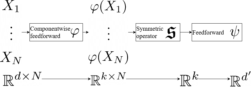
for 𝒚𝒚{\boldsymbol{y}} == (yi)i1,Nsubscriptsubscript𝑦𝑖𝑖1𝑁(y_{i})_{i\in\llbracket 1,N\rrbracket} \in (k)Nsuperscriptsuperscript𝑘𝑁(\operatorname{\mathbb{R}}^{k})^{N}. When 𝔰𝔰\mathfrak{s} is the max-pooling function, 𝒮d,,m,k,d𝔰,N,ρsuperscriptsubscript𝒮𝑑𝑚𝑘superscript𝑑𝔰𝑁𝜌{\cal S}_{d,\ell,m,k,d^{\prime}}^{\mathfrak{s},N,\rho} is called PointNet, as introduced in [RQ+17], while for 𝔰𝔰\mathfrak{s} equals to the sum/average function, it is called DeepSet, see [Zah+17]. The architecture is described in Figure 1, and k𝑘k can be interpreted as a number of features describing the geometry of the set of points {xi}i1,Nsubscriptsubscript𝑥𝑖𝑖1𝑁\{x_{i}\}_{i\in\llbracket 1,N\rrbracket}. For example in the context of mean-field control problem, k𝑘k will be related to the moments for describing the law of the McKean-Vlasov SDE.

A given symmetric network function 𝒰𝒰{\cal U} \in 𝒮d,,m,k,d𝔰,N,ρsubscriptsuperscript𝒮𝔰𝑁𝜌𝑑𝑚𝑘superscript𝑑{\cal S}^{\mathfrak{s},N,\rho}_{d,\ell,m,k,d^{\prime}} is determined by the weight/bias parameters θ𝜃\theta == (θ(1),θ(2))superscript𝜃1superscript𝜃2(\theta^{(1)},\theta^{(2)}) with θ(1)superscript𝜃1\theta^{(1)} == (𝒲0(1),β0(1),,𝒲(1),β(1))superscriptsubscript𝒲01superscriptsubscript𝛽01superscriptsubscript𝒲1superscriptsubscript𝛽1({\cal W}_{0}^{(1)},\beta_{0}^{(1)},\ldots,{\cal W}_{\ell}^{(1)},\beta_{\ell}^{(1)}) defining the layer functions ϕ0,ϕsubscriptitalic-ϕ0subscriptitalic-ϕ\phi_{0}\ldots,\phi_{\ell} of φ𝜑\varphi, and θ(2)superscript𝜃2\theta^{(2)} == (𝒲0(2),β0(2),,𝒲(2),β(2))superscriptsubscript𝒲02superscriptsubscript𝛽02superscriptsubscript𝒲2superscriptsubscript𝛽2({\cal W}_{0}^{(2)},\beta_{0}^{(2)},\ldots,{\cal W}_{\ell}^{(2)},\beta_{\ell}^{(2)}) defining the layer functions ψ0,ψsubscript𝜓0subscript𝜓\psi_{0}\ldots,\psi_{\ell} of ψ𝜓\psi. The number of parameters is M𝑀M == M1+M2subscript𝑀1subscript𝑀2M_{1}+M_{2}, with M1subscript𝑀1M_{1} == m(d+1)+m(m+1)(1)+(m+1)k𝑚𝑑1𝑚𝑚11𝑚1𝑘m(d+1)+m(m+1)(\ell-1)+(m+1)k, M2subscript𝑀2M_{2} == (k+1)m+m(m+1)(1)+(m+1)d𝑘1𝑚𝑚𝑚11𝑚1superscript𝑑(k+1)m+m(m+1)(\ell-1)+(m+1)d^{\prime}, and we observe that it does not depend on the number N𝑁N of inputs.

Refer to caption
Figure 1: Architecture of a symmetric neural network.
Remark 3.1 (Time dependent symmetric network).

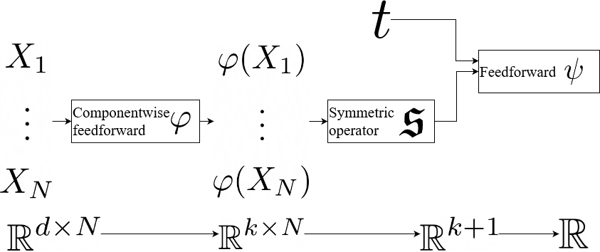
A time-dependent symmetric in space neural network can be constructed as

𝒰(t,𝒙)𝒰𝑡𝒙\displaystyle{\cal U}(t,{\boldsymbol{x}}) =\displaystyle= ψ(t,𝔰((φ(xi))i1,N)), for t+,𝒙=(xi)iI(d)N,formulae-sequence𝜓𝑡𝔰subscript𝜑subscript𝑥𝑖𝑖1𝑁 for 𝑡subscript𝒙subscriptsubscript𝑥𝑖𝑖𝐼superscriptsuperscript𝑑𝑁\displaystyle\psi\big{(}t,\mathfrak{s}((\varphi(x_{i}))_{i\in\llbracket 1,N\rrbracket})\big{)},\quad\mbox{ for }t\in\operatorname{\mathbb{R}}_{+},\;{\boldsymbol{x}}=(x_{i})_{i\in I}\in(\operatorname{\mathbb{R}}^{d})^{N}, (3.5)

with φ𝜑\varphi a feedforward network from dsuperscript𝑑\operatorname{\mathbb{R}}^{d} into ksuperscript𝑘\operatorname{\mathbb{R}}^{k}, and ψ𝜓\psi is a feedforward from k+1superscript𝑘1\operatorname{\mathbb{R}}^{k+1} into dsuperscriptsuperscript𝑑\operatorname{\mathbb{R}}^{d^{\prime}}, where we add time as an additional feature, see architecture in Figure 2.
Refer to caption
Figure 2: Architecture of time dependent symmetric network.

\Box

A D𝐷D-symmetric neural network function, denoted 𝒵𝒵{\cal Z} \in D𝒮d,,m,k,d𝔰,N,ρ𝐷subscriptsuperscript𝒮𝔰𝑁𝜌𝑑𝑚𝑘superscript𝑑D{\cal S}^{\mathfrak{s},N,\rho}_{d,\ell,m,k,d^{\prime}}, is an dsuperscriptsuperscript𝑑\operatorname{\mathbb{R}}^{d^{\prime}}-valued D𝐷D-exchangeable function in the form

𝒵(𝒙,x)𝒵𝒙𝑥\displaystyle{\cal Z}({\boldsymbol{x}},x) =ψ(𝔰((φ(xi))i1,N),x), for 𝒙=(xi)i1,N(d)N,xd,formulae-sequenceformulae-sequenceabsent𝜓𝔰subscript𝜑subscript𝑥𝑖𝑖1𝑁𝑥 for 𝒙subscriptsubscript𝑥𝑖𝑖1𝑁superscriptsuperscript𝑑𝑁𝑥superscript𝑑\displaystyle=\;\psi\big{(}\mathfrak{s}((\varphi(x_{i}))_{i\in\llbracket 1,N\rrbracket}),x\big{)},\quad\mbox{ for }{\boldsymbol{x}}=(x_{i})_{i\in\llbracket 1,N\rrbracket}\in(\operatorname{\mathbb{R}}^{d})^{N},x\in\operatorname{\mathbb{R}}^{d}, (3.6)

where φ𝜑\varphi \in 𝒩d,,m,kρsuperscriptsubscript𝒩𝑑𝑚𝑘𝜌{\cal N}_{d,\ell,m,k}^{\rho}, ψ𝜓\psi \in 𝒩k+d,,m,dρsuperscriptsubscript𝒩𝑘𝑑𝑚superscript𝑑𝜌{\cal N}_{k+d,\ell,m,d^{\prime}}^{\rho}, and 𝔰𝔰\mathfrak{s} is a given ksuperscript𝑘\operatorname{\mathbb{R}}^{k}-valued N𝑁N-exchangeable function on ksuperscript𝑘\operatorname{\mathbb{R}}^{k}. The number of parameters of a given 𝒵𝒵{\cal Z} \in D𝒮d,,m,k,d𝔰,ρ𝐷subscriptsuperscript𝒮𝔰𝜌𝑑𝑚𝑘superscript𝑑D{\cal S}^{\mathfrak{s},\rho}_{d,\ell,m,k,d^{\prime}} is Msuperscript𝑀M^{\prime} == M1+M2subscriptsuperscript𝑀1subscriptsuperscript𝑀2M^{\prime}_{1}+M^{\prime}_{2}, with M1subscriptsuperscript𝑀1M^{\prime}_{1} == m(d+1)+m(m+1)(1)+(m+1)k𝑚𝑑1𝑚𝑚11𝑚1𝑘m(d+1)+m(m+1)(\ell-1)+(m+1)k, M2subscriptsuperscript𝑀2M^{\prime}_{2} == m(k+d+1)+m(m+1)(1)+(m+1)d𝑚𝑘𝑑1𝑚𝑚11𝑚1superscript𝑑m(k+d+1)+m(m+1)(\ell-1)+(m+1)d^{\prime}. We shall often take for 𝔰𝔰\mathfrak{s} the average function, and call D𝒮d,,m,k,d𝔰,N,ρ𝐷subscriptsuperscript𝒮𝔰𝑁𝜌𝑑𝑚𝑘superscript𝑑D{\cal S}^{\mathfrak{s},N,\rho}_{d,\ell,m,k,d^{\prime}} as DeepDerSet. Its architecture is given in Figure 3. Given a D𝐷D-symmetric neural network 𝒵𝒵{\cal Z}, we denote by 𝓩𝓩{\boldsymbol{{\cal Z}}} the function defined on (d)Nsuperscriptsuperscript𝑑𝑁(\operatorname{\mathbb{R}}^{d})^{N} by 𝓩(𝒙)𝓩𝒙{\boldsymbol{{\cal Z}}}({\boldsymbol{x}}) == (𝒵(𝒙,xi))1,Nsubscript𝒵𝒙subscript𝑥𝑖absent1𝑁({\cal Z}({\boldsymbol{x}},x_{i}))_{\in\llbracket 1,N\rrbracket} \in (d)Nsuperscriptsuperscript𝑑𝑁(\operatorname{\mathbb{R}}^{d})^{N}, and by misuse of notation, we may also call 𝓩𝓩{\boldsymbol{{\cal Z}}} as a D𝐷D-symmetric NN. By construction, these networks respect the representation given by Lemma 2.5, by being defined as a D𝐷D-exchangeable function applied component by component. In that way we are able to enforce the correct symmetries for representing both a symmetric function and its derivative, which will be useful in Section 4 and Section 5 when looking for the gradient of PDE solutions.

Refer to caption
Figure 3: Architecture of DeepDerSet network

Alternatively, one can generate D𝐷D-exchangeable functions as follows. Starting from a DeepSet element 𝒰𝒰{\cal U} \in 𝒮d,,m,k,d𝔰,N,ρsuperscriptsubscript𝒮𝑑𝑚𝑘superscript𝑑𝔰𝑁𝜌{\cal S}_{d,\ell,m,k,d^{\prime}}^{\mathfrak{s},N,\rho} as in (3.4) with 𝔰𝔰\mathfrak{s} the sum function, and network functions φ,ψ𝜑𝜓\varphi,\psi with smooth activation functions

Dxi𝒰(𝒙)subscript𝐷subscript𝑥𝑖𝒰𝒙\displaystyle D_{x_{i}}{\cal U}({\boldsymbol{x}}) =D𝒰(𝒙,xi),𝒙=(xi)1,N(d)N,formulae-sequenceabsentD𝒰𝒙subscript𝑥𝑖𝒙subscriptsubscript𝑥𝑖absent1𝑁superscriptsuperscript𝑑𝑁\displaystyle={\rm D}{\cal U}({\boldsymbol{x}},x_{i}),\quad{\boldsymbol{x}}=(x_{i})_{\in\llbracket 1,N\rrbracket}\in(\operatorname{\mathbb{R}}^{d})^{N}, (3.7)

with

D𝒰(𝒙,x)D𝒰𝒙𝑥\displaystyle{\rm D}{\cal U}({\boldsymbol{x}},x) :=Dφ(x)Dψ(𝔰((φ(xi))iI)),xd.formulae-sequenceassignabsent𝐷𝜑𝑥𝐷𝜓𝔰subscript𝜑subscript𝑥𝑖𝑖𝐼𝑥superscript𝑑\displaystyle:=\;D\varphi(x)D\psi\big{(}\mathfrak{s}((\varphi(x_{i}))_{i\in I})\big{)},\quad x\in\operatorname{\mathbb{R}}^{d}. (3.8)

The set of D𝐷D-exchangeable functions obtained from differentiation of DeepSet network functions is called AD-DeepSet, where AD stands for automatic differentiation, and Automatic refers to the implementation of the differentiation in software library, e.g. in TensorFlow. This alternative network for approximating the derivative of a differentiable symmetric function naturally respects the structure given by Lemma 2.5, by construction as the derivative of a symmetric DeepSet neural network.

Given a D𝐷D-symmetric NN 𝓩𝓩{\boldsymbol{{\cal Z}}} in DeepDerSet or in AD-DeepSet with smooth activation functions, we denote by D𝓩𝐷𝓩D{\boldsymbol{{\cal Z}}} its differentiation.

As for the well-known universal approximation theorem [Hor91] for neural networks, we have a similar result for symmetric neural networks, which states that any exchangeable function can be arbitrarily approximated by a PointNet or DeepSet given enough neurons. More precisely, by combining Theorem 2.9 of [Wag+19] with Theorem 2 of [Hor91], we obtain the following approximation theorem for DeepSets.

Universal approximation for DeepSets networks. Let 𝔰𝔰\mathfrak{s} be the sum function. The set m=1𝒮d,,m,N+1,d𝔰,N,ρsuperscriptsubscript𝑚1subscriptsuperscript𝒮𝔰𝑁𝜌𝑑𝑚𝑁1superscript𝑑\cup_{m=1}^{\infty}{\cal S}^{\mathfrak{s},N,\rho}_{d,\ell,m,N+1,d^{\prime}} approximates any N𝑁N-exchangeable continuous function w𝑤w arbitrary well on any compact set of K𝐾K \subset dsuperscript𝑑\operatorname{\mathbb{R}}^{d}, once ρ𝜌\rho is continuous, bounded and non-constant: for all ε𝜀\varepsilon >> 00, N𝑁N \in superscript\mathbb{N}^{*}, there exists 𝒰𝒰{\cal U} \in m=1𝒮d,,m,N+1,d𝔰,N,ρsuperscriptsubscript𝑚1subscriptsuperscript𝒮𝔰𝑁𝜌𝑑𝑚𝑁1superscript𝑑\cup_{m=1}^{\infty}{\cal S}^{\mathfrak{s},N,\rho}_{d,\ell,m,N+1,d^{\prime}} such that

|w(𝒙)𝒰(𝒙)|𝑤𝒙𝒰𝒙\displaystyle\big{|}w({\boldsymbol{x}})-{\cal U}({\boldsymbol{x}})\big{|} ε𝒙KN.formulae-sequenceabsent𝜀for-all𝒙superscript𝐾𝑁\displaystyle\leq\;\varepsilon\quad\forall{\boldsymbol{x}}\in K^{N}. (3.9)

Note that a priori the latent space dimension k𝑘k has to be chosen equal to N+1𝑁1N+1.

Alternatively, by combining Theorem 1 of [RQ+17] with Theorem 2 of [Hor91], we obtain the following one-dimensional approximation theorem for PointNet.

Universal approximation for PointNet networks. Let 𝔰𝔰\mathfrak{s} be the max\max function. The set m=1k=1𝒮1,,m,k,d𝔰,N,ρ\cup_{m=1}^{\infty}\cup_{k=1}^{\infty}{\cal S}^{\mathfrak{s},N,\rho}_{1,\ell,m,k,d^{\prime}} approximates any N𝑁N-exchangeable Hausdorff continuous function w𝑤w (seen as a function on sets) arbitrary well on any compact set of K𝐾K \subset \operatorname{\mathbb{R}} , once ρ𝜌\rho is continuous, bounded, and non-constant: for all ε𝜀\varepsilon >> 00, N𝑁N \in superscript\mathbb{N}^{*}, there exists 𝒰𝒰{\cal U} \in m=1k=1𝒮1,,m,k,d𝔰,N,ρ\cup_{m=1}^{\infty}\cup_{k=1}^{\infty}{\cal S}^{\mathfrak{s},N,\rho}_{1,\ell,m,k,d^{\prime}} such that

|w(S)𝒰(𝒙)|𝑤𝑆𝒰𝒙\displaystyle\big{|}w(S)-{\cal U}({\boldsymbol{x}})\big{|} ε,SK,S={x1,,xN}.formulae-sequenceabsent𝜀formulae-sequencefor-all𝑆𝐾𝑆subscript𝑥1subscript𝑥𝑁\displaystyle\leq\;\varepsilon,\quad\forall S\subset K,\ S=\{x_{1},\cdots,x_{N}\}. (3.10)

Note here that a priori the latent space dimension k𝑘k has to be chosen as large as needed.

3.2 Comparison tests

In this paragraph, we test the accuracy of the approximation of exchangeable functions by DeepSet or PointNet, and also the approximation of D𝐷D-exchangeable functions by DeepDerSet or AD-DeepSet, and compare numerically with classical feedforward approximations.

3.2.1 Approximation of some simple functions

We first test the approximation of the following simple symmetric functions:

  1. 1.

    f(x)𝑓𝑥f(x) == exp(2x¯+3x¯3)2¯𝑥3superscript¯𝑥3\exp{(2\bar{x}+3\bar{x}^{3})}, with x¯¯𝑥\bar{x} == 1Ni=1Nxi1𝑁superscriptsubscript𝑖1𝑁subscript𝑥𝑖\displaystyle{\frac{1}{N}\sum_{i=1}^{N}x_{i}} (case 1)

  2. 2.

    f(x)𝑓𝑥f(x) == 1Ni=1N[sin(xi)1xi<0+xi1xi0]1𝑁superscriptsubscript𝑖1𝑁delimited-[]subscript𝑥𝑖subscript1subscript𝑥𝑖0subscript𝑥𝑖subscript1subscript𝑥𝑖0\displaystyle{\frac{1}{N}\sum_{i=1}^{N}}\big{[}\sin(x_{i})1_{x_{i}<0}+x_{i}1_{x_{i}\geq 0}\big{]} (case 2)

  3. 3.

    f(x)𝑓𝑥f(x) == x¯+2x¯2+3x¯3¯𝑥2superscript¯𝑥23superscript¯𝑥3\bar{x}+2\bar{x}^{2}+3\bar{x}^{3}, with x¯¯𝑥\bar{x} == max{xi,i=1,,N}subscript𝑥𝑖𝑖1𝑁\max\{x_{i},i=1,\dots,N\} (case 3)

  4. 4.

    f(x)𝑓𝑥f(x) == cos(2x¯+3x¯2)2¯𝑥3superscript¯𝑥2\cos(2\bar{x}+3\bar{x}^{2}), with x¯¯𝑥\bar{x} == i=1Nxisuperscriptsubscript𝑖1𝑁subscript𝑥𝑖\sum_{i=1}^{N}x_{i} (case 4)

We use a symmetric neural network architecture as proposed in [RQ+17], [Zah+17]:

  • First, a feedforward network φ𝜑\varphi with \ell == 555 hidden layers, and respectively 64,64,64,12864646412864,64,64,128 and 102410241024 neurons such that each dimension i𝑖i, i=1,,N𝑖1𝑁i=1,\dots,N, is treated with the same network in one dimension avoiding to break the symmetry.

  • Two possible symmetric functions 𝔰𝔰\mathfrak{s} to the order N𝑁N on ksuperscript𝑘\operatorname{\mathbb{R}}^{k} with k𝑘k == 102410241024, the max-pooling (PointNet) and the sum function (DeepSet).

  • At last, a feedforward network ψ𝜓\psi from 1024superscript1024\operatorname{\mathbb{R}}^{1024} to \operatorname{\mathbb{R}} with \ell == 222 hidden layers, and respectively 512512512 and 256256256 neurons.

For the approximation with classical feedforward networks, we used three or four layers and a number of neurons constant per layer equal to 10+d10𝑑10+d, or 10+2d102𝑑10+2d neurons.

We use the ADAM optimizer ([KB14]), with a batch size equal to 300300300 for solving the approximation problem with quadratic loss function:

minθ𝔼[|f(X)𝒰θ(X)|2],subscript𝜃𝔼delimited-[]superscript𝑓𝑋superscript𝒰𝜃𝑋2\displaystyle\min_{\theta}\mathbb{E}[|f(X)-{\cal U}^{\theta}(X)|^{2}], (3.11)

with training simulations from X𝑋X similar-to\sim 𝒩(0N,1N)𝒩subscript0𝑁subscript1𝑁{\cal N}(0_{N},1_{N}), and θ𝜃\theta are the parameters of the network function 𝒰θsuperscript𝒰𝜃{\cal U}^{\theta}. The number of epochs (corresponding to the number of gradient descent iterations) used is equal to 100100100. After epoch iterations of the stochastic gradient, the error (3.11) is estimated with 200002000020000 simulations. If the error is below a threshold equal to 1e51E-5110-5 the optimization is stopped, otherwise a counter for outer iterations is incremented. The number of outer iterations is blocked at epochExt =1000absent1000=1000 (meaning a maximal total number of stochastic gradient iterations equal to epoch ×\times epochExt =100000absent100000=100000).

In Tables 1, 2, 3, we report the accuracy reached (Error) and the number of iterations (Iter.) used to obtain this given accuracy: then a threshold equal to 1e51E-5110-5 means that the optimization has been successful and the relevant parameter is the number of iterations used. A number of iterations equal to expochExt == 100010001000 means that the optimization has not been successful and the error reached indicates how far we are from optimality. For the feedforward case, we report the best result (“minimum” in table) and the worse result (“maximum” in table) obtained changing the number of layers and the number of neurons used.

The initial learning rate is taken equal to 1e31E-3110-3 for first outer simulation in cases 1 and 2 with a linear decay to 1e51E-5110-5 for a number of outer iterations equal to 100010001000. For test case 3, the initial learning rate is taken equal to 1e41E-4110-4 with a linear decay to 1e51E-5110-5. The result obtained in Table 1 is similarly obtained with a large number of functions tested in dimension between N𝑁N == 101010 to 100010001000. It shows the following results:

  • The classical feedforward, with dense layers, often permits to obtain optimally without forcing symmetry of the solution,

  • Classical feedforward results do not depend a lot on the number of layers, the number of neurons tested and the activation function used,

  • For symmetric approximations, DeepSets generally permits to get the best results and the ReLU activation function is the best out of the three tested.

Symmetric Feedforward
PointNet DeepSet Minimum Maximum
Activation Error Iter. Error Iter. Error Iter. Error Iter.
ReLU 0.0080.0080.008 100010001000 1e51E-5110-5 101010 1e51E-5110-5 125125125 1e51E-5110-5 166166166
tanh 0.0160.0160.016 100010001000 1e51E-5110-5 288288288 1e51E-5110-5 180180180 1e51E-5110-5 308308308
ELU 0.0150.0150.015 100010001000 1e51E-5110-5 176176176 1e51E-5110-5 108108108 1e51E-5110-5 130130130
Table 1: Approximation error (3.11) obtained for different networks on one run and number of iterations used depending on activation functions for approximation of the function f𝑓f in case 1, dimension N𝑁N == 100100100.

In the sequel, we drop the ELU activation function on other cases as shown in Tables 2 for cases 2 and 3. Notice that case 3, involving a max function is the only one where PointNet approximation gives the best result among the other tested networks. On cases 2 and 3 in dimension 100, the DeepSets approximation outperforms the classical feedforward network for all the number of layers and neurons tested. However, results on case 3 are not very good for the PointNet approximation even with the ReLU activation function.

Case activ Symmetric Feedforward
PointNet DeepSets Minimum Maximum
Error Iter. Error Iter. Error Iter. Error Iter.
2 ReLU 0.0010.0010.001 100010001000 1e51E-5110-5 555 1e51E-5110-5 992992992 0.0020.0020.002 100010001000
2 tanh 0.030.030.03 100010001000 1e51E-5110-5 342342342 0.00180.00180.0018 100010001000 6×6\times 1e51E-5110-5 100010001000
3 ReLU 0.0010.0010.001 100010001000 0.230.230.23 100010001000 888888 100010001000 432432432 100010001000
3 tanh 0.0020.0020.002 100010001000 656565 100010001000 933933933 100010001000 969969969 100010001000
Table 2: Approximation error (3.11) obtained for different networks on one run and number of iterations used for approximation of the function f𝑓f in cases 2 and 3, dimension N𝑁N == 100100100, activation function ReLU.

Results for test case 4 are given on Table 3 using an initial learning rate equal to 5e55E-5510-5 and a decay linear to 5e65E-6510-6 with the number of outer iterations.

Symmetric Feedforward
PointNet DeepSets Minimum Maximum
activ Error Iter. Error Iter. Error Iter. Error Iter.
ReLU 0.19100.19100.1910 100010001000 8.9e58.9E-58.910-5 100010001000 0.00450.00450.0045 100010001000 0.010.010.01 100010001000
tanh 0.190.190.19 100010001000 4e54E-5410-5 100010001000 0.00060.00060.0006 100010001000 0.00120.00120.0012 100010001000
Table 3: Approximation error (3.11) obtained for different networks, activation functions for approximation of the function f𝑓f in case 4 dimension 1000.

At last, considering case 4 in dimension N𝑁N == 100010001000, when the function is quickly changing, we see that the classical feedforward network functions have difficulty to converge while the DeepSets network approximation converges. The latter turns out to be a very good candidate to some very high dimensional PDEs when there is symmetry in the solution.

3.2.2 Approximation of a function of t𝑡t and x𝑥x with symmetry in x𝑥x

We test the accuracy of our time dependent symmetric neural network by considering the following two cases of functions:

  1. 1.

    f(x)=exp(x¯(t+2t2)+3tx¯3)𝑓𝑥¯𝑥𝑡2superscript𝑡23𝑡superscript¯𝑥3f(x)=\exp\big{(}\bar{x}(t+2t^{2})+3t\bar{x}^{3}\big{)} with x¯¯𝑥\bar{x} == 1Ni=1Nxi1𝑁superscriptsubscript𝑖1𝑁subscript𝑥𝑖\displaystyle{\frac{1}{N}\sum_{i=1}^{N}x_{i}} (case 1)

  2. 2.

    f(x)=t+cos(tx¯)𝑓𝑥𝑡𝑡¯𝑥f(x)=t+\cos(t\bar{x}), with x¯¯𝑥\bar{x} == 1Ni=1Nxi1𝑁superscriptsubscript𝑖1𝑁subscript𝑥𝑖\frac{1}{\sqrt{N}}\sum_{i=1}^{N}x_{i} (case 2)

The approximation is performed through the minimization problem

minθ𝔼[|f(τ,X)𝒰θ(τ,X)|2],subscript𝜃𝔼delimited-[]superscript𝑓𝜏𝑋superscript𝒰𝜃𝜏𝑋2\displaystyle\min_{\theta}\mathbb{E}[|f(\tau,X)-{\cal U}^{\theta}(\tau,X)|^{2}], (3.12)

with training simulations from X𝒩(0N,1N)similar-to𝑋𝒩subscript0𝑁subscript1𝑁X\sim{\cal N}(0_{N},1_{N}), and an independent uniform law for τ𝜏\tau on [0,1]01[0,1], and where 𝒰θsuperscript𝒰𝜃{\cal U}^{\theta} is a time-dependent DeepSet with parameters θ𝜃\theta. We keep the same number of neurons and layers as in the previous section, and compare with a classical feedforward network composed of 333 layers of d+10𝑑10d+10 neurons. In all experiments, we use a ReLU activation function.

Case DeepSets Feedforward
Error Iter. Error Iter.
1 1e51E-5110-5 676767 0.0080.0080.008 100010001000
2 1e51E-5110-5 344344344 0.0480.0480.048 100010001000
Table 4: Approximation error (3.12) obtained for different networks on one run and number of iterations used for approximation of the function f𝑓f in case 1 and 2, dimension N𝑁N == 100100100.

In Table 4, we give the results obtained in dimension 100. Surprisingly, the feedforward approximation seems to have difficulties to approximate the case 1 although it is quite similar to case one in the previous section. As for the second case, the result is not so surprising as the case is quite similar to case 4 in previous section, where the feedforward network has difficulties to converge.

3.2.3 Gradient approximation

We now focus on the approximation of the derivative of an exchangeable function by means of 𝒰θsuperscript𝒰𝜃{\cal U}^{\theta} a DeepDerSet, a AD-DeepSet, or a classical feedforward network .

The minimization problem is now:

minθ𝔼[Df(X)𝒰θ(X)2],subscript𝜃𝔼delimited-[]superscriptnorm𝐷𝑓𝑋superscript𝒰𝜃𝑋2\displaystyle\min_{\theta}\mathbb{E}[\|Df(X)-{\cal U}^{\theta}(X)\|^{2}], (3.13)

where the norm \|\cdot\| is the Euclidean norm.

The comparison is performed on the following test functions:

  1. 1.

    f(x)𝑓𝑥f(x) == exp(x¯+x¯3)(1N+3x2)¯𝑥superscript¯𝑥3subscript1𝑁3superscript𝑥2\exp{(\bar{x}+\bar{x}^{3})}(1_{N}+3x^{2}) where x¯¯𝑥\bar{x} == 1Ni=1Nxi1𝑁superscriptsubscript𝑖1𝑁subscript𝑥𝑖\displaystyle{\frac{1}{N}\sum_{i=1}^{N}x_{i}} (case 1)

  2. 2.

    f(x)𝑓𝑥f(x) == y𝑦y where yi=1xi>0+cos(xi)1xi<0,i=1,,Nformulae-sequencesubscript𝑦𝑖subscript1subscript𝑥𝑖0𝑐𝑜𝑠subscript𝑥𝑖subscript1subscript𝑥𝑖0𝑖1𝑁y_{i}=1_{x_{i}>0}+cos(x_{i})1_{x_{i}<0},\quad i=1,\dots,N (case 2)

  3. 3.

    f(x)𝑓𝑥f(x) == 1Nsin(x¯)1N1𝑁¯𝑥subscript1𝑁\frac{1}{\sqrt{N}}\sin(\bar{x})1_{N}, where x¯¯𝑥\bar{x} == 1Ni=1Nxi1𝑁superscriptsubscript𝑖1𝑁subscript𝑥𝑖\frac{1}{\sqrt{N}}\sum_{i=1}^{N}x_{i} (case 3)

We compare the classical feedforward approximation to our network approximation in Tables 5 and 6, using a maximal number of iterations equal to 500050005000. Clearly using a ReLU activation function is superior to the tanh activation function and the DeepDerSet gives the best approximation while the AD-DeepSet or the feedforward may have difficulties to approximate the functions accurately.

Case N𝑁N Feedforward DeepDerSet AD-DeepSet
Error Iter. Error Iter. Error Iter.
1 10 5e45E-4510-4 5000 5e45E-4510-4 5000 7e37E-3710-3 5000
1 100 1e51E-5110-5 300 1e51E-5110-5 250 1e51E-5110-5 50
2 10 0.030.030.03 5000 1e51E-5110-5 550 2e42E-4210-4 5000
2 100 0.120.120.12 5000 1e51E-5110-5 450 1e41E-4110-4 5000
3 10 1e51E-5110-5 3800 1e51E-5110-5 850 0.030.030.03 5000
3 100 1e51E-5110-5 1850 1e51E-5110-5 700 3e33E-3310-3 5000
Table 5: Approximation error (3.13) with ReLU activation function obtained for different networks on one run and number of iterations used for approximation of the derivative of an exchangeable function.
Case N𝑁N Feedforward DeepDerSet AD-DeepSet
Error Iter. Error Iter. Error Iter.
1 10 5e45E-4510-4 5000 1.7e41.7E-41.710-4 5000 3e33E-3310-3 5000
1 100 1e51E-5110-5 500 1e51E-5110-5 100 1e51E-5110-5 50
2 10 0.030.030.03 5000 1e51E-5110-5 950 0.0280.0280.028 5000
2 100 0.120.120.12 5000 1e51E-5110-5 700 0.560.560.56 5000
3 10 1.5e51.5E-51.510-5 5000 1e51E-5110-5 1850 0.020.020.02 5000
3 100 1e51E-5110-5 2100 1e51E-5110-5 1350 4e34E-3410-3 5000
Table 6: Approximation error (3.13) with tanh activation function obtained for different networks on one run and number of iterations used for approximation of the derivative of an exchangeable function.

4 Numerical schemes

We now adapt the deep backward dynamic programming (DBDP) schemes developed in [HPW20] and [PWG21] for solving nonlinear PDEs, by using symmetric neural networks and D𝐷D-symmetric neural networks (instead of feedforward neural networks) for approximating the exchangeable solution v𝑣v and its gradient D𝒙vsubscript𝐷𝒙𝑣D_{{\boldsymbol{x}}}v. We recall the main steps of the DBDP scheme, and distinguish the case of semi-linear and fully non-linear PDEs.

4.1 Semi-linear PDE

We first consider the case where the generator F𝐹F in (2.1) may be decomposed into the form

F(t,𝒙,y,𝒛,𝜸)𝐹𝑡𝒙𝑦𝒛𝜸\displaystyle F(t,{\boldsymbol{x}},y,{\boldsymbol{z}},{\boldsymbol{\gamma}}) =\displaystyle= H(t,𝒙,y,𝒛)+i=1Nbi(t,𝒙).zi+12i,j=1Ntr(Σij(t,𝒙)γij),formulae-sequence𝐻𝑡𝒙𝑦𝒛superscriptsubscript𝑖1𝑁subscript𝑏𝑖𝑡𝒙subscript𝑧𝑖12superscriptsubscript𝑖𝑗1𝑁trsubscriptΣ𝑖𝑗𝑡𝒙subscript𝛾𝑖𝑗\displaystyle H(t,{\boldsymbol{x}},y,{\boldsymbol{z}})+\sum_{i=1}^{N}b_{i}(t,{\boldsymbol{x}}).z_{i}+\frac{1}{2}\sum_{i,j=1}^{N}{\rm tr}\big{(}\Sigma_{ij}(t,{\boldsymbol{x}})\gamma_{ij}\big{)}, (4.1)

for t𝑡t \in [0,T]0𝑇[0,T], 𝒙𝒙{\boldsymbol{x}} == (xi)i1,Nsubscriptsubscript𝑥𝑖𝑖1𝑁(x_{i})_{i\in\llbracket 1,N\rrbracket} \in (d)Nsuperscriptsuperscript𝑑𝑁(\operatorname{\mathbb{R}}^{d})^{N}, y𝑦y \in \operatorname{\mathbb{R}}, 𝒛𝒛{\boldsymbol{z}} == (zi)i1,Nsubscriptsubscript𝑧𝑖𝑖1𝑁(z_{i})_{i\in\llbracket 1,N\rrbracket} \in (d)Nsuperscriptsuperscript𝑑𝑁(\operatorname{\mathbb{R}}^{d})^{N}, and 𝜸𝜸{\boldsymbol{\gamma}} == (γij)i,j1,Nsubscriptsubscript𝛾𝑖𝑗𝑖𝑗1𝑁(\gamma_{ij})_{i,j\in\llbracket 1,N\rrbracket} \in 𝕊N(𝕊d)superscript𝕊𝑁superscript𝕊𝑑\mathbb{S}^{N}(\mathbb{S}^{d}). Here, H𝐻H is a function on [0,T]×(d)N××(d)N0𝑇superscriptsuperscript𝑑𝑁superscriptsuperscript𝑑𝑁[0,T]\times(\operatorname{\mathbb{R}}^{d})^{N}\times\operatorname{\mathbb{R}}\times(\operatorname{\mathbb{R}}^{d})^{N} satisfying the permutation-invariance condition:

H(t,𝒙,y,𝒛)𝐻𝑡𝒙𝑦𝒛\displaystyle H(t,{\boldsymbol{x}},y,{\boldsymbol{z}}) =\displaystyle= H(t,π[𝒙],y,π[𝒛]),π𝔖N,𝐻𝑡𝜋delimited-[]𝒙𝑦𝜋delimited-[]𝒛for-all𝜋subscript𝔖𝑁\displaystyle H(t,\pi[{\boldsymbol{x}}],y,\pi[{\boldsymbol{z}}]),\quad\forall\pi\in\mathfrak{S}_{N},

the coefficients bisubscript𝑏𝑖b_{i}, i𝑖i == 1,,N1𝑁1,\ldots,N, are dsuperscript𝑑\operatorname{\mathbb{R}}^{d}-valued functions on [0,T]×(d)N0𝑇superscriptsuperscript𝑑𝑁[0,T]\times(\operatorname{\mathbb{R}}^{d})^{N} satisfying the condition

bi(t,π[𝒙])subscript𝑏𝑖𝑡𝜋delimited-[]𝒙\displaystyle b_{i}(t,\pi[{\boldsymbol{x}}]) =bπ(i)(t,𝒙),π𝔖N,formulae-sequenceabsentsubscript𝑏𝜋𝑖𝑡𝒙for-all𝜋subscript𝔖𝑁\displaystyle=\;b_{\pi(i)}(t,{\boldsymbol{x}}),\quad\forall\pi\in\mathfrak{S}_{N}, (4.2)

and the coefficients ΣijsubscriptΣ𝑖𝑗\Sigma_{ij}, i,j𝑖𝑗i,j == 1,,N1𝑁1,\ldots,N, are d×d𝑑𝑑d\times d-matrix valued functions on [0,T]×(d)N0𝑇superscriptsuperscript𝑑𝑁[0,T]\times(\operatorname{\mathbb{R}}^{d})^{N} in the form

Σij(t,𝒙)subscriptΣ𝑖𝑗𝑡𝒙\displaystyle\Sigma_{ij}(t,{\boldsymbol{x}}) =σijσij(t,𝒙)+σi0σj0(t,𝒙),absentsubscript𝜎𝑖𝑗superscriptsubscript𝜎𝑖𝑗𝑡𝒙subscript𝜎𝑖0subscriptsuperscript𝜎𝑗0𝑡𝒙\displaystyle=\;\sigma_{ij}\sigma_{ij}^{\scriptscriptstyle{\intercal}}(t,{\boldsymbol{x}})+\sigma_{i0}\sigma^{\scriptscriptstyle{\intercal}}_{j0}(t,{\boldsymbol{x}}), (4.3)

for some d×d𝑑𝑑d\times d-matrix valued functions σijsubscript𝜎𝑖𝑗\sigma_{ij}, and d×q𝑑𝑞d\times q-matrix valued functions σi0subscript𝜎𝑖0\sigma_{i0}, satisfying the invariance property: for all π𝜋\pi \in 𝔖Nsubscript𝔖𝑁\mathfrak{S}_{N},

σij(t,π[𝒙])=σπ(i)π(j)(t,𝒙),σi0(t,π[𝒙])=σπ(i)0(t,𝒙).formulae-sequencesubscript𝜎𝑖𝑗𝑡𝜋delimited-[]𝒙subscript𝜎𝜋𝑖𝜋𝑗𝑡𝒙subscript𝜎𝑖0𝑡𝜋delimited-[]𝒙subscript𝜎𝜋𝑖0𝑡𝒙\sigma_{ij}(t,\pi[{\boldsymbol{x}}])\;=\;\sigma_{\pi(i)\pi(j)}(t,{\boldsymbol{x}}),\quad\quad\sigma_{i0}(t,\pi[{\boldsymbol{x}}])\;=\;\sigma_{\pi(i)0}(t,{\boldsymbol{x}}). (4.4)

In this case, the permutation-invariance condition (HI) on F𝐹F is satisfied, and we observe that it includes Example 2.1 of multi-asset pricing with H(t,𝒙,y,𝒛)𝐻𝑡𝒙𝑦𝒛H(t,{\boldsymbol{x}},y,{\boldsymbol{z}}) == β(y+y)𝛽superscript𝑦𝑦\beta(y^{+}-y) (in the case of the CVA pricing), bisubscript𝑏𝑖b_{i} \equiv r𝑟r and σi0subscript𝜎𝑖0\sigma_{i0} \equiv 00. This also includes Example 2.2 of the McKean-Vlasov control problem under common noise with uncontrolled diffusion coefficient, where σij(t,𝒙)subscript𝜎𝑖𝑗𝑡𝒙\sigma_{ij}(t,{\boldsymbol{x}}) == σ(t,xi,μ¯(𝒙))δij𝜎𝑡subscript𝑥𝑖¯𝜇𝒙subscript𝛿𝑖𝑗\sigma(t,x_{i},\bar{\mu}({\boldsymbol{x}}))\delta_{ij}, σi0(t,𝒙)subscript𝜎𝑖0𝑡𝒙\sigma_{i0}(t,{\boldsymbol{x}}) == σ0(t,xi,μ¯(𝒙))subscript𝜎0𝑡subscript𝑥𝑖¯𝜇𝒙\sigma_{0}(t,x_{i},\bar{\mu}({\boldsymbol{x}})), and

H(t,𝒙,y,𝒛)𝐻𝑡𝒙𝑦𝒛\displaystyle H(t,{\boldsymbol{x}},y,{\boldsymbol{z}}) =ry+i=1NinfaA[β(t,xi,μ¯(𝒙),a).zi+1Nf(xi,μ¯(𝒙),a)]\displaystyle=-ry+\sum_{i=1}^{N}\inf_{a\in A}\big{[}\beta(t,x_{i},\bar{\mu}({\boldsymbol{x}}),a).z_{i}+\frac{1}{N}f(x_{i},\bar{\mu}({\boldsymbol{x}}),a)\big{]} (4.5)
i=1Nbi(t,𝒙).zi,formulae-sequencesuperscriptsubscript𝑖1𝑁subscript𝑏𝑖𝑡𝒙subscript𝑧𝑖\displaystyle\quad\quad\quad-\sum_{i=1}^{N}b_{i}(t,{\boldsymbol{x}}).z_{i}, (4.6)

for any function bisubscript𝑏𝑖b_{i} satisfying (4.2). We shall discuss more in detail the relevant choice of the drift coefficient bisubscript𝑏𝑖b_{i} in Section 4.3.

The starting point of the numerical scheme is the probabilistic representation of the PDE (2.1) with F𝐹F as in (4.1) in terms of a forward backward stochastic differential equation (FBSDE), as in [PP90]. In our context, the forward system is described by the process 𝑿𝑿{\boldsymbol{X}} == (X1,,XN)superscript𝑋1superscript𝑋𝑁(X^{1},\ldots,X^{N}) valued in (d)Nsuperscriptsuperscript𝑑𝑁(\operatorname{\mathbb{R}}^{d})^{N} governed by the diffusion dynamics:

dXti𝑑superscriptsubscript𝑋𝑡𝑖\displaystyle dX_{t}^{i} =bi(t,𝑿t)dt+j=0Nσij(t,𝑿t)dWtj,absentsubscript𝑏𝑖𝑡subscript𝑿𝑡𝑑𝑡superscriptsubscript𝑗0𝑁subscript𝜎𝑖𝑗𝑡subscript𝑿𝑡𝑑superscriptsubscript𝑊𝑡𝑗\displaystyle=\;b_{i}(t,{\boldsymbol{X}}_{t})dt+\sum_{j=0}^{N}\sigma_{ij}(t,{\boldsymbol{X}}_{t})dW_{t}^{j}, (4.7)

where Wisuperscript𝑊𝑖W^{i}, i𝑖i == 1,,N1𝑁1,\ldots,N, are independent d𝑑d-dimensional Brownian motions, independent of the q𝑞q-dimensional Brownian motion W0superscript𝑊0W^{0}. Given this forward diffusion process, we then consider the pair process (Y,𝒁=(Zi)i1,N)𝑌𝒁subscriptsuperscript𝑍𝑖𝑖1𝑁(Y,{\boldsymbol{Z}}=(Z^{i})_{i\in\llbracket 1,N\rrbracket}) valued in ×(d)Nsuperscriptsuperscript𝑑𝑁\operatorname{\mathbb{R}}\times(\operatorname{\mathbb{R}}^{d})^{N} solution to the BSDE

G(𝑿T)Yt+tTH(s,𝑿s,Ys,𝒁s)𝑑s𝐺subscript𝑿𝑇subscript𝑌𝑡superscriptsubscript𝑡𝑇𝐻𝑠subscript𝑿𝑠subscript𝑌𝑠subscript𝒁𝑠differential-d𝑠\displaystyle G({\boldsymbol{X}}_{T})-Y_{t}+\int_{t}^{T}H(s,{\boldsymbol{X}}_{s},Y_{s},{\boldsymbol{Z}}_{s})ds (4.8)
i=1Nj=0NtT(Zsi)σij(s,𝑿s)𝑑Wsjsuperscriptsubscript𝑖1𝑁superscriptsubscript𝑗0𝑁superscriptsubscript𝑡𝑇superscriptsuperscriptsubscript𝑍𝑠𝑖subscript𝜎𝑖𝑗𝑠subscript𝑿𝑠differential-dsuperscriptsubscript𝑊𝑠𝑗\displaystyle-\sum_{i=1}^{N}\sum_{j=0}^{N}\int_{t}^{T}(Z_{s}^{i})^{\scriptscriptstyle{\intercal}}\sigma_{ij}(s,{\boldsymbol{X}}_{s})dW_{s}^{j} = 0,0tT,formulae-sequenceabsent 00𝑡𝑇\displaystyle\;=\;0,\quad\quad 0\leq t\leq T, (4.9)

which is connected by Itô’s formula to the solution of the PDE (2.1) via:

Yt=v(t,𝑿t),subscript𝑌𝑡𝑣𝑡subscript𝑿𝑡\displaystyle Y_{t}\;=\;v(t,{\boldsymbol{X}}_{t}), Zti=Dxiv(t,𝑿t),i=1,,N,0tT.formulae-sequencesuperscriptsubscript𝑍𝑡𝑖subscript𝐷subscript𝑥𝑖𝑣𝑡subscript𝑿𝑡formulae-sequence𝑖1𝑁0𝑡𝑇\displaystyle Z_{t}^{i}\;=\;D_{x_{i}}v(t,{\boldsymbol{X}}_{t}),\;i=1,\ldots,N,\quad 0\leq t\leq T.

We next consider a time discretization of this FBSDE on a time grid {tk,k=0,,NT}formulae-sequencesubscript𝑡𝑘𝑘0subscript𝑁𝑇\{t_{k},k=0,\ldots,N_{T}\}, with t0subscript𝑡0t_{0} == 00, tNTsubscript𝑡subscript𝑁𝑇t_{N_{T}} == T𝑇T, ΔtkΔsubscript𝑡𝑘\Delta t_{k} :=assign:= tk+1tksubscript𝑡𝑘1subscript𝑡𝑘t_{k+1}-t_{k} >> 00, by defining the Euler scheme {𝑿kNT=(Xki,NT)i1,N\{{\boldsymbol{X}}_{k}^{N_{T}}=(X_{k}^{i,N_{T}})_{i\in\llbracket 1,N\rrbracket}, k=0,,NT}k=0,\ldots,N_{T}\} associated to the forward diffusion process {𝑿t=(Xti)i1,N\{{\boldsymbol{X}}_{t}=(X_{t}^{i})_{i\in\llbracket 1,N\rrbracket}, 0tT}0\leq t\leq T\}, which is used for the training simulations, together with the increments of the Brownian motions: ΔWkjΔsuperscriptsubscript𝑊𝑘𝑗\Delta W_{k}^{j} :=assign:= Wtk+1jWtkjsuperscriptsubscript𝑊subscript𝑡𝑘1𝑗superscriptsubscript𝑊subscript𝑡𝑘𝑗W_{t_{k+1}}^{j}-W_{t_{k}}^{j}, k𝑘k == 0,,NT10subscript𝑁𝑇10,\ldots,N_{T}-1, j𝑗j == 0,,N0𝑁0,\ldots,N, of our numerical backward scheme. The DBDP algorithm reads then as follows:

Initialization: Initialize from the exchangeable function: 𝒰^NT()subscript^𝒰subscript𝑁𝑇\widehat{\cal U}_{N_{T}}(\cdot) == G()𝐺G(\cdot)
for  k𝑘k == NT1,,0subscript𝑁𝑇10N_{T}-1,\ldots,0 do
      minimize over symmetric NN 𝒰ksubscript𝒰𝑘{\cal U}_{k}, and D𝐷D-symmetric NN 𝒵ksubscript𝒵𝑘{\cal Z}_{k}, the quadratic loss function
J1(𝒰k,𝒵k)subscript𝐽1subscript𝒰𝑘subscript𝒵𝑘\displaystyle J_{1}({\cal U}_{k},{\cal Z}_{k}) =𝔼|𝒰^k+1(𝑿k+1NT)𝒰k(𝑿kNT)absentconditional𝔼subscript^𝒰𝑘1superscriptsubscript𝑿𝑘1subscript𝑁𝑇subscript𝒰𝑘superscriptsubscript𝑿𝑘subscript𝑁𝑇\displaystyle=\;\mathbb{E}\Big{|}\widehat{\cal U}_{k+1}({\boldsymbol{X}}_{k+1}^{N_{T}})-{\cal U}_{k}({\boldsymbol{X}}_{k}^{N_{T}}) (4.10)
+H(tk,𝑿kNT,𝒰k(𝑿kNT),𝓩k(𝑿kNT))Δtk𝐻subscript𝑡𝑘superscriptsubscript𝑿𝑘subscript𝑁𝑇subscript𝒰𝑘superscriptsubscript𝑿𝑘subscript𝑁𝑇subscript𝓩𝑘superscriptsubscript𝑿𝑘subscript𝑁𝑇Δsubscript𝑡𝑘\displaystyle\quad\quad\quad+\;H\big{(}t_{k},{\boldsymbol{X}}_{k}^{N_{T}},{\cal U}_{k}({\boldsymbol{X}}_{k}^{N_{T}}),{\boldsymbol{{\cal Z}}}_{k}({\boldsymbol{X}}_{k}^{N_{T}})\big{)}\Delta t_{k} (4.11)
i=1Nj=0N(𝒵k(𝑿kNT,Xki,NT))σij(tk,𝑿kNT)ΔWkj|2,\displaystyle\quad\quad\quad-\;\sum_{i=1}^{N}\sum_{j=0}^{N}\big{(}{\cal Z}_{k}({\boldsymbol{X}}_{k}^{N_{T}},X_{k}^{i,N_{T}})\big{)}^{\scriptscriptstyle{\intercal}}\sigma_{ij}\big{(}t_{k},{\boldsymbol{X}}_{k}^{N_{T}}\big{)}\Delta W_{k}^{j}\Big{|}^{2}, (4.12)
and update (𝒰^k,𝒵^k)subscript^𝒰𝑘subscript^𝒵𝑘(\widehat{\cal U}_{k},\widehat{\cal Z}_{k}) as the solution to this minimization problem.
end for
Algorithm 1 DBDP scheme with symmetric NN

The output of the DBDP scheme provides approximations 𝒰^k(𝒙)subscript^𝒰𝑘𝒙\widehat{\cal U}_{k}({\boldsymbol{x}}) of v(tk,𝒙)𝑣subscript𝑡𝑘𝒙v(t_{k},{\boldsymbol{x}}), and 𝓩^k(𝒙)subscript^𝓩𝑘𝒙\widehat{\boldsymbol{{\cal Z}}}_{k}({\boldsymbol{x}}) of D𝒙v(tk,𝒙)subscript𝐷𝒙𝑣subscript𝑡𝑘𝒙D_{{\boldsymbol{x}}}v(t_{k},{\boldsymbol{x}}), k𝑘k == 0,,NT10subscript𝑁𝑇10,\ldots,N_{T}-1, for values of 𝒙𝒙{\boldsymbol{x}} \in (d)Nsuperscriptsuperscript𝑑𝑁(\operatorname{\mathbb{R}}^{d})^{N} that are well-explored by the training simulations of 𝑿kNTsuperscriptsubscript𝑿𝑘subscript𝑁𝑇{\boldsymbol{X}}_{k}^{N_{T}}. We refer to [PWG21] (see their section 3.1) for a discussion on the choice of the algorithm hyperparameters.

Remark 4.1.

We stress that the neural networks do not take time as an input. Adding time would not make any difference because the training is done locally, time step per time step. So the neural networks approximating 𝒰ksubscript𝒰𝑘{\cal U}_{k} and 𝒵ksubscript𝒵𝑘{\cal Z}_{k} would be trained with only tksubscript𝑡𝑘t_{k} as an input and hence they would not be able to learn the dependence on time. However, at time k<NT𝑘subscript𝑁𝑇k<N_{T}, we initialize the parameters of 𝒰ksubscript𝒰𝑘{\cal U}_{k} and 𝒵ksubscript𝒵𝑘{\cal Z}_{k} respectively with the parameters of the neural networks for 𝒰k+1subscript𝒰𝑘1{\cal U}_{k+1} and 𝒵k+1subscript𝒵𝑘1{\cal Z}_{k+1}, which have been trained at the previous iteration. This gives a good initial guess for the neural networks at time tksubscript𝑡𝑘t_{k} and leads to more efficient training.

4.2 Fully nonlinear PDE

We consider more generally the fully non-linear PDE (2.1) with a symmetric generator F𝐹F satisfying (HI). We adapt the machine learning scheme in [PWG21] for solving fully nonlinear PDEs by exploiting furthermore the exchangeability property of the solution by using again symmetric neural networks as in the semi-linear case.

We fix some arbitrary drift and diffusion coefficients bisubscript𝑏𝑖b_{i}, σijsubscript𝜎𝑖𝑗\sigma_{ij}, i𝑖i == 1,,N1𝑁1,\ldots,N, j𝑗j == 0,,N0𝑁0,\ldots,N, satisfying invariance properties as in (4.2)-(4.4) (in practice, they should be chosen depending on the studied problem as for the semi-linear case, see a general discussion in Section 3.1 in [PWG21], and an application in Section 5.3), and introduce the forward diffusion system 𝑿𝑿{\boldsymbol{X}} as in (4.7) and its discrete-time Euler scheme 𝑿NTsuperscript𝑿subscript𝑁𝑇{\boldsymbol{X}}^{N_{T}}. We then consider the triple process (Y,𝒁=(Zi)i1,N,𝚪=(Γij)i,j1,N)formulae-sequence𝑌𝒁subscriptsuperscript𝑍𝑖𝑖1𝑁𝚪subscriptsuperscriptΓ𝑖𝑗𝑖𝑗1𝑁(Y,{\boldsymbol{Z}}=(Z^{i})_{i\in\llbracket 1,N\rrbracket},{\boldsymbol{\Gamma}}=(\Gamma^{ij})_{i,j\in\llbracket 1,N\rrbracket}) valued in ×(d)N×𝕊N(𝕊d)superscriptsuperscript𝑑𝑁superscript𝕊𝑁superscript𝕊𝑑\operatorname{\mathbb{R}}\times(\operatorname{\mathbb{R}}^{d})^{N}\times\mathbb{S}^{N}(\mathbb{S}^{d}) solution to the BSDE

G(𝑿T)Yt+tTFb,σ(s,𝑿s,Ys,𝒁s,𝚪s)𝑑s𝐺subscript𝑿𝑇subscript𝑌𝑡superscriptsubscript𝑡𝑇subscript𝐹𝑏𝜎𝑠subscript𝑿𝑠subscript𝑌𝑠subscript𝒁𝑠subscript𝚪𝑠differential-d𝑠\displaystyle G({\boldsymbol{X}}_{T})-Y_{t}+\int_{t}^{T}F_{b,\sigma}(s,{\boldsymbol{X}}_{s},Y_{s},{\boldsymbol{Z}}_{s},{\boldsymbol{\Gamma}}_{s})ds (4.13)
i=1Nj=0NtT(Zsi)σij(s,𝑿s)𝑑Wsjsuperscriptsubscript𝑖1𝑁superscriptsubscript𝑗0𝑁superscriptsubscript𝑡𝑇superscriptsuperscriptsubscript𝑍𝑠𝑖subscript𝜎𝑖𝑗𝑠subscript𝑿𝑠differential-dsuperscriptsubscript𝑊𝑠𝑗\displaystyle-\sum_{i=1}^{N}\sum_{j=0}^{N}\int_{t}^{T}(Z_{s}^{i})^{\scriptscriptstyle{\intercal}}\sigma_{ij}(s,{\boldsymbol{X}}_{s})dW_{s}^{j} = 0,0tT,formulae-sequenceabsent 00𝑡𝑇\displaystyle=\;0,\quad 0\leq t\leq T, (4.14)

with

Fb,σ(t,𝒙,y,𝒛,𝜸)subscript𝐹𝑏𝜎𝑡𝒙𝑦𝒛𝜸\displaystyle F_{b,\sigma}(t,{\boldsymbol{x}},y,{\boldsymbol{z}},{\boldsymbol{\gamma}}) :=F(t,𝒙,y,𝒛,𝜸)i=1Nbi(t,𝒙).zi12i,j=1Ntr(Σij(t,𝒙)γij),formulae-sequenceassignabsent𝐹𝑡𝒙𝑦𝒛𝜸superscriptsubscript𝑖1𝑁subscript𝑏𝑖𝑡𝒙subscript𝑧𝑖12superscriptsubscript𝑖𝑗1𝑁trsubscriptΣ𝑖𝑗𝑡𝒙subscript𝛾𝑖𝑗\displaystyle:=\;F(t,{\boldsymbol{x}},y,{\boldsymbol{z}},{\boldsymbol{\gamma}})-\sum_{i=1}^{N}b_{i}(t,{\boldsymbol{x}}).z_{i}-\frac{1}{2}\sum_{i,j=1}^{N}{\rm tr}\big{(}\Sigma_{ij}(t,{\boldsymbol{x}})\gamma_{ij}\big{)}, (4.15)

and ΣijsubscriptΣ𝑖𝑗\Sigma_{ij} as in (4.3). It is connected by Itô’s formula to the fully non-linear PDE (2.1) via the representation: Ytsubscript𝑌𝑡Y_{t} == v(t,𝑿t)𝑣𝑡subscript𝑿𝑡v(t,{\boldsymbol{X}}_{t}), 𝒁tsubscript𝒁𝑡{\boldsymbol{Z}}_{t} == D𝒙v(t,𝑿t)subscript𝐷𝒙𝑣𝑡subscript𝑿𝑡D_{{\boldsymbol{x}}}v(t,{\boldsymbol{X}}_{t}), 𝚪tsubscript𝚪𝑡{\boldsymbol{\Gamma}}_{t} == D𝒙2v(t,𝑿t)superscriptsubscript𝐷𝒙2𝑣𝑡subscript𝑿𝑡D_{{\boldsymbol{x}}}^{2}v(t,{\boldsymbol{X}}_{t}), 0tT0𝑡𝑇0\leq t\leq T.

Assuming that G𝐺G is smooth, the algorithm is designed in Algorithm 2.

Initialization: Initialize from the exchangeable function: 𝒰^NT()subscript^𝒰subscript𝑁𝑇\widehat{\cal U}_{N_{T}}(\cdot) == G()𝐺G(\cdot) and the D𝐷D-exchangeable function 𝓩^NT()subscript^𝓩subscript𝑁𝑇\widehat{\boldsymbol{{\cal Z}}}_{N_{T}}(\cdot) == DG()𝐷𝐺DG(\cdot).
for  k𝑘k == NT1,,0subscript𝑁𝑇10N_{T}-1,\ldots,0 do
      minimize over symmetric NN 𝒰ksubscript𝒰𝑘{\cal U}_{k}, and D𝐷D-symmetric NN 𝒵ksubscript𝒵𝑘{\cal Z}_{k}, the quadratic loss function
J2(𝒰k,𝒵k)subscript𝐽2subscript𝒰𝑘subscript𝒵𝑘\displaystyle J_{2}({\cal U}_{k},{\cal Z}_{k}) =𝔼|𝒰^k+1(𝑿k+1NT)𝒰k(𝑿kNT)absentconditional𝔼subscript^𝒰𝑘1superscriptsubscript𝑿𝑘1subscript𝑁𝑇subscript𝒰𝑘superscriptsubscript𝑿𝑘subscript𝑁𝑇\displaystyle=\;\mathbb{E}\Big{|}\widehat{\cal U}_{k+1}({\boldsymbol{X}}_{k+1}^{N_{T}})-{\cal U}_{k}({\boldsymbol{X}}_{k}^{N_{T}}) (4.16)
+Fb,σ(tk,𝑿kNT,𝒰k(𝑿kNT),𝓩k(𝑿kNT),D𝓩^k+1(𝑿k+1NT))Δtksubscript𝐹𝑏𝜎subscript𝑡𝑘superscriptsubscript𝑿𝑘subscript𝑁𝑇subscript𝒰𝑘superscriptsubscript𝑿𝑘subscript𝑁𝑇subscript𝓩𝑘superscriptsubscript𝑿𝑘subscript𝑁𝑇𝐷subscript^𝓩𝑘1superscriptsubscript𝑿𝑘1subscript𝑁𝑇Δsubscript𝑡𝑘\displaystyle\quad\quad\quad+\;F_{b,\sigma}\big{(}t_{k},{\boldsymbol{X}}_{k}^{N_{T}},{\cal U}_{k}({\boldsymbol{X}}_{k}^{N_{T}}),{\boldsymbol{{\cal Z}}}_{k}({\boldsymbol{X}}_{k}^{N_{T}}),D\widehat{\boldsymbol{{\cal Z}}}_{k+1}({\boldsymbol{X}}_{k+1}^{N_{T}})\big{)}\Delta t_{k} (4.17)
i=1Nj=0N(𝒵k(𝑿kNT,Xki,NT))σij(tk,𝑿kNT)ΔWkj|2,\displaystyle\quad\quad\quad-\;\sum_{i=1}^{N}\sum_{j=0}^{N}\big{(}{\cal Z}_{k}({\boldsymbol{X}}_{k}^{N_{T}},X_{k}^{i,N_{T}})\big{)}^{\scriptscriptstyle{\intercal}}\sigma_{ij}\big{(}t_{k},{\boldsymbol{X}}_{k}^{N_{T}}\big{)}\Delta W_{k}^{j}\Big{|}^{2}, (4.18)
and update (𝒰^k,𝒵^k)subscript^𝒰𝑘subscript^𝒵𝑘(\widehat{\cal U}_{k},\widehat{\cal Z}_{k}) as the solution to this minimization problem. Here D𝓩^k+1Dsubscript^𝓩𝑘1{\rm D}\widehat{\boldsymbol{{\cal Z}}}_{k+1} is the automatic differentiation of the D𝐷D-symmetric NN 𝓩^k+1subscript^𝓩𝑘1\widehat{\boldsymbol{{\cal Z}}}_{k+1} computed previously at the time step k+1𝑘1k+1.
end for
Algorithm 2 Fully nonlinear DPBD scheme with symmetric NN

4.3 The case of mean-field PDEs

We consider in this section the case where the PDE (2.1) is the particles approximation of a McKean-Vlasov control problem with a Bellman equation (2.5) in the Wasserstein space of probability measures as described in Example 2.2. To simplify the presentation, we consider that there is only control on the drift coefficient β(t,x,μ,a)𝛽𝑡𝑥𝜇𝑎\beta(t,x,\mu,a) but no control on the diffusion coefficient σ(t,x,μ)𝜎𝑡𝑥𝜇\sigma(t,x,\mu) and σ0(t,x,μ)subscript𝜎0𝑡𝑥𝜇\sigma_{0}(t,x,\mu) of the McKean-Vlasov equation (2.4). In this case, recall that when the solution v(t,μ)𝑣𝑡𝜇v(t,\mu) to this Bellman equation is smooth, an optimal control is given in feedback form by (see [PW17]):

αtsuperscriptsubscript𝛼𝑡\displaystyle\alpha_{t}^{*} =\displaystyle= a^(t,Xt,Xt0,μv(t,Xt0)(Xt)),^𝑎𝑡superscriptsubscript𝑋𝑡subscriptsuperscript0superscriptsubscript𝑋𝑡subscript𝜇𝑣𝑡subscriptsuperscript0superscriptsubscript𝑋𝑡superscriptsubscript𝑋𝑡\displaystyle\hat{a}(t,X_{t}^{*},\mathbb{P}^{0}_{{}_{X_{t}^{*}}},\partial_{\mu}v(t,\mathbb{P}^{0}_{{}_{X_{t}^{*}}})(X_{t}^{*})),

where a^(t,x,μ,z)^𝑎𝑡𝑥𝜇𝑧\hat{a}(t,x,\mu,z) is an argmin\min of a𝑎a \in A𝐴A maps-to\mapsto β(t,x,μ,a).z+f(x,μ,a)formulae-sequence𝛽𝑡𝑥𝜇𝑎𝑧𝑓𝑥𝜇𝑎\beta(t,x,\mu,a).z+f(x,\mu,a), and Xsuperscript𝑋X^{*} == Xαsuperscript𝑋superscript𝛼X^{\alpha^{*}} is the optimal McKean-Vlasov state process.

Approximation of the optimal control by forward induction of the scheme. As proven in [GPW22], the solution (𝑿,Y,𝒁)𝑿𝑌𝒁({\boldsymbol{X}},Y,{\boldsymbol{Z}}) to the FBSDE (4.7)-(4.8) provides an approximation with a rate of convergence 1/N1𝑁1/N, when N𝑁N goes to infinity, of the solution v𝑣v to (2.5), and its L𝐿L-derivative: Ytsubscript𝑌𝑡Y_{t} similar-to-or-equals\simeq v(t,μ¯(𝑿t))𝑣𝑡¯𝜇subscript𝑿𝑡v(t,\bar{\mu}({\boldsymbol{X}}_{t})), NZti𝑁superscriptsubscript𝑍𝑡𝑖NZ_{t}^{i} similar-to-or-equals\simeq μv(t,μ¯(𝑿t))(Xti)subscript𝜇𝑣𝑡¯𝜇subscript𝑿𝑡superscriptsubscript𝑋𝑡𝑖\partial_{\mu}v(t,\bar{\mu}({\boldsymbol{X}}_{t}))(X_{t}^{i}). The drift coefficients bisubscript𝑏𝑖b_{i} of the forward particles system 𝑿𝑿{\boldsymbol{X}} should be chosen in order to generate from training simulations a suitable exploration of the state space for getting a good approximation of the optimal feedback control. In practice, in a first step, one can choose bi(t,𝒙)subscript𝑏𝑖𝑡𝒙b_{i}(t,{\boldsymbol{x}}) == β(t,xi,μ¯(𝒙),a0)𝛽𝑡subscript𝑥𝑖¯𝜇𝒙subscript𝑎0\beta(t,x_{i},\bar{\mu}({\boldsymbol{x}}),a_{0}), for some arbitrary value a0subscript𝑎0a_{0} \in A𝐴A of the control. After a first implementation of Algorithm 1, we thus have an approximation of μv(t,μ)(x)subscript𝜇𝑣𝑡𝜇𝑥\partial_{\mu}v(t,\mu)(x) at time t𝑡t == tksubscript𝑡𝑘t_{k}, and μ𝜇\mu == μ¯(𝒙)¯𝜇𝒙\bar{\mu}({\boldsymbol{x}}), by N𝒵^k(𝒙,x)𝑁subscript^𝒵𝑘𝒙𝑥N\widehat{\cal Z}_{k}({\boldsymbol{x}},x). Notice however that we solved the PDE along the law of the forward training process, which is different from the optimally controlled process law, except at the initial time t0subscript𝑡0t_{0}, where we then get an approximation of the optimal feedback control with

(x,μ¯(𝒙))𝑥¯𝜇𝒙\displaystyle(x,\bar{\mu}({\boldsymbol{x}})) a^(t0,x,μ¯(𝒙),N𝒵^0(𝒙,x)).absent^𝑎subscript𝑡0𝑥¯𝜇𝒙𝑁subscript^𝒵0𝒙𝑥\displaystyle\longmapsto\;\hat{a}(t_{0},x,\bar{\mu}({\boldsymbol{x}}),N\widehat{\cal Z}_{0}({\boldsymbol{x}},x)). (4.19)

Next, by defining an updated initial drift coefficient as

b^i(t0,𝒙)subscript^𝑏𝑖subscript𝑡0𝒙\displaystyle\hat{b}_{i}(t_{0},{\boldsymbol{x}}) :=β(t0,xi,μ¯(𝒙),a^(t0,xi,μ¯(𝒙),N𝒵^0(𝒙,xi))), for 𝒙=(xi)i1,N,i=1,,N,formulae-sequenceassignabsent𝛽subscript𝑡0subscript𝑥𝑖¯𝜇𝒙^𝑎subscript𝑡0subscript𝑥𝑖¯𝜇𝒙𝑁subscript^𝒵0𝒙subscript𝑥𝑖formulae-sequence for 𝒙subscriptsubscript𝑥𝑖𝑖1𝑁𝑖1𝑁\displaystyle:=\;\beta\big{(}t_{0},x_{i},\bar{\mu}({\boldsymbol{x}}),\hat{a}(t_{0},x_{i},\bar{\mu}({\boldsymbol{x}}),N\widehat{\cal Z}_{0}({\boldsymbol{x}},x_{i}))\big{)},\;\mbox{ for }{\boldsymbol{x}}=(x_{i})_{i\in\llbracket 1,N\rrbracket},\;i=1,\ldots,N, (4.20)

and considering the N𝑁N-particle discrete-time system {𝑿^kNT=(X^ki,NT)i1,N,k=0,,NT}formulae-sequencesuperscriptsubscript^𝑿𝑘subscript𝑁𝑇subscriptsuperscriptsubscript^𝑋𝑘𝑖subscript𝑁𝑇𝑖1𝑁𝑘0subscript𝑁𝑇\{\hat{\boldsymbol{X}}_{k}^{N_{T}}=(\hat{X}_{k}^{i,N_{T}})_{i\in\llbracket 1,N\rrbracket},k=0,\ldots,N_{T}\}, starting from i.i.d. samples X0isuperscriptsubscript𝑋0𝑖X_{0}^{i}, i𝑖i == 1,,N1𝑁1,\ldots,N distributed according to some distribution μ0subscript𝜇0\mu_{0} on dsuperscript𝑑\operatorname{\mathbb{R}}^{d}, and with dynamics

X^1i,NTsubscriptsuperscript^𝑋𝑖subscript𝑁𝑇1\displaystyle\hat{X}^{i,N_{T}}_{1} =X0i+b^i(t0,𝑿0)Δt0+σ(t0,X0i,μ¯(𝑿0))ΔW0i,absentsubscriptsuperscript𝑋𝑖0subscript^𝑏𝑖subscript𝑡0subscript𝑿0Δsubscript𝑡0𝜎subscript𝑡0superscriptsubscript𝑋0𝑖¯𝜇subscript𝑿0Δsuperscriptsubscript𝑊0𝑖\displaystyle=\;X^{i}_{0}+\hat{b}_{i}(t_{0},{\boldsymbol{X}}_{0})\Delta t_{0}+\sigma(t_{0},X_{0}^{i},\bar{\mu}({\boldsymbol{X}}_{0}))\Delta W_{0}^{i}, (4.21)
X^k+1i,NTsubscriptsuperscript^𝑋𝑖subscript𝑁𝑇𝑘1\displaystyle\hat{X}^{i,N_{T}}_{k+1} =X^ki,NT+bi(tk,𝑿kNT)Δtk+σ(tk,X^ki,NT,μ¯(𝑿^kNT))ΔWki,absentsubscriptsuperscript^𝑋𝑖subscript𝑁𝑇𝑘subscript𝑏𝑖subscript𝑡𝑘superscriptsubscript𝑿𝑘subscript𝑁𝑇Δsubscript𝑡𝑘𝜎subscript𝑡𝑘subscriptsuperscript^𝑋𝑖subscript𝑁𝑇𝑘¯𝜇superscriptsubscript^𝑿𝑘subscript𝑁𝑇Δsuperscriptsubscript𝑊𝑘𝑖\displaystyle=\;\hat{X}^{i,N_{T}}_{k}+b_{i}(t_{k},{\boldsymbol{X}}_{k}^{N_{T}})\Delta t_{k}+\sigma(t_{k},\hat{X}^{i,N_{T}}_{k},\bar{\mu}(\hat{{\boldsymbol{X}}}_{k}^{N_{T}}))\Delta W_{k}^{i}, (4.22)

for k𝑘k == 1,,NT11subscript𝑁𝑇11,\ldots,N_{T}-1, we obtain an approximation of the distribution of the optimal particle mean-field process at time t1subscript𝑡1t_{1}. Applying the algorithm again between t1subscript𝑡1t_{1} and tNTsubscript𝑡subscript𝑁𝑇t_{N_{T}} then allows to compute an approximation of the optimal feedback control a^(t1,x,μ¯(𝒙),𝒵^1(𝒙,x))^𝑎subscript𝑡1𝑥¯𝜇𝒙subscript^𝒵1𝒙𝑥\hat{a}(t_{1},x,\bar{\mu}({\boldsymbol{x}}),\widehat{\cal Z}_{1}({\boldsymbol{x}},x)) at time t1subscript𝑡1t_{1} and to update the simulation of X^2i,NTsubscriptsuperscript^𝑋𝑖subscript𝑁𝑇2\hat{X}^{i,N_{T}}_{2}. By induction, we can compute the optimal feedback control at every time step through NTsubscript𝑁𝑇N_{T} executions of the scheme.

Approximation of the solution by randomization of the training simulations. Algorithm 1 provides actually an approximation of v(t,μ)𝑣𝑡𝜇v(t,\mu) (resp. μv(t,μ)(x)subscript𝜇𝑣𝑡𝜇𝑥\partial_{\mu}v(t,\mu)(x)) at time tksubscript𝑡𝑘t_{k}, and for empirical measures μ𝜇\mu == μ¯(𝒙)¯𝜇𝒙\bar{\mu}({\boldsymbol{x}}), by 𝒰^k(𝒙)subscript^𝒰𝑘𝒙\widehat{\cal U}_{k}({\boldsymbol{x}}) (resp. N𝒵^k(𝒙,x)𝑁subscript^𝒵𝑘𝒙𝑥N\widehat{\cal Z}_{k}({\boldsymbol{x}},x)). Thus, in order to get an approximation of v(tk,.)v(t_{k},.) (resp. μv(tk,.)(x)\partial_{\mu}v(t_{k},.)(x)) on the whole Wasserstein space 𝒫2(d)subscript𝒫2superscript𝑑{\cal P}_{2}(\operatorname{\mathbb{R}}^{d}), we need a suitable exploration of μ¯(𝑿kNT)¯𝜇superscriptsubscript𝑿𝑘subscript𝑁𝑇\bar{\mu}({\boldsymbol{X}}_{k}^{N_{T}}) when using the training simulations 𝑿kNTsuperscriptsubscript𝑿𝑘subscript𝑁𝑇{\boldsymbol{X}}_{k}^{N_{T}}, k𝑘k == 0,,NT0subscript𝑁𝑇0,\ldots,N_{T}. For that purpose, some randomization can first be implemented by randomizing the initial law μ0subscript𝜇0\mu_{0} of the forward process. By sampling μ0subscript𝜇0\mu_{0} in a compact set K𝐾K of 𝒫2(d)subscript𝒫2superscript𝑑{\cal P}_{2}(\operatorname{\mathbb{R}}^{d}) for each batch element, such as a family of Gaussian measures for instance, our algorithm will be able to learn the value function v(0,μ)𝑣0𝜇v(0,\mu) and its Lions derivative μv(0,μ)subscript𝜇𝑣0𝜇\partial_{\mu}v(0,\mu) on K𝐾K. Therefore, instead of solving the PDE several times for each initial law we can run the algorithm only once. This can be useful if we have an uncertainty in the initial law of the problem we aim to solve. It corresponds to learning the solution v(tk,μk,¯)𝑣subscript𝑡𝑘¯subscript𝜇𝑘v(t_{k},\overline{\mu_{k,\ell}}) on a family of empirical measures corresponding to forward processes Xi,(),NTsuperscript𝑋𝑖subscript𝑁𝑇X^{i,(\ell),N_{T}}, i𝑖i == 1,,N1𝑁1,\ldots,N, with initial laws μ0Ksuperscriptsubscript𝜇0𝐾\mu_{0}^{\ell}\in K. Relying on the generalization properties of neural networks, we expect to approximate the value function at time t0subscript𝑡0t_{0} == 00 on K𝐾K. Furthermore, if the goal is to obtain an approximation of the PDE solution at any time step tksubscript𝑡𝑘t_{k}, the task is more complex. A randomization needs to be performed at each time step tksubscript𝑡𝑘t_{k} by sampling 𝑿kNTsubscriptsuperscript𝑿subscript𝑁𝑇𝑘{\boldsymbol{X}}^{N_{T}}_{k} according to a Gaussian mixture νksubscript𝜈𝑘\nu_{k} with random parameters. We then apply Algorithm 1, and expect to learn the solution over measures with regular densities. The updated method is presented in Algorithm 3. If the state space exploration is efficient, the feedback control will be directly available with only one execution of the algorithm, contrarily to the previously described procedure with NTsubscript𝑁𝑇N_{T} executions. We should explore the Wasserstein space well enough to learn the value function and its derivative on the unknown law of the optimal process.

Initialization: Initialize from the exchangeable function: 𝒰^NT()subscript^𝒰subscript𝑁𝑇\widehat{\cal U}_{N_{T}}(\cdot) == G()𝐺G(\cdot)
for  k𝑘k == NT1,,0subscript𝑁𝑇10N_{T}-1,\ldots,0 do
      define random variables
LU(1,Lmax),φlU(0,1),μiU(μmax,μmax),(θi)2U(0,σmax2)formulae-sequencesimilar-to𝐿𝑈1subscript𝐿𝑚𝑎𝑥formulae-sequencesimilar-tosubscript𝜑𝑙𝑈01formulae-sequencesimilar-tosubscript𝜇𝑖𝑈subscript𝜇𝑚𝑎𝑥subscript𝜇𝑚𝑎𝑥similar-tosuperscriptsubscript𝜃𝑖2𝑈0superscriptsubscript𝜎𝑚𝑎𝑥2L\sim U(1,L_{max}),\ \varphi_{l}\sim U(0,1),\ \mu_{i}\sim U(-\mu_{max},\mu_{max}),\ (\theta_{i})^{2}\sim U(0,\sigma_{max}^{2})
       define a random Gaussian mixture νksubscript𝜈𝑘\nu_{k} of random density
l=1Lφl𝒩(μi,θi2)l=1Lφlsuperscriptsubscript𝑙1𝐿subscript𝜑𝑙𝒩subscript𝜇𝑖superscriptsubscript𝜃𝑖2superscriptsubscript𝑙1𝐿subscript𝜑𝑙\frac{\sum_{l=1}^{L}\varphi_{l}{\cal N}(\mu_{i},\theta_{i}^{2})}{\sum_{l=1}^{L}\varphi_{l}}
       define N𝑁N i.i.d. particles Xki,NTsubscriptsuperscript𝑋𝑖subscript𝑁𝑇𝑘X^{i,N_{T}}_{k} with law νksubscript𝜈𝑘\nu_{k} for i=1,,N𝑖1𝑁i=1,\cdots,N,
       perform one Euler-Maruyama scheme step
Xk+1i,NTsubscriptsuperscript𝑋𝑖subscript𝑁𝑇𝑘1\displaystyle X^{i,N_{T}}_{k+1} =Xki,NT+bi(tk,𝑿kNT)Δtk+σ(tk,Xki,NT,μ¯(𝑿kNT))ΔWki,absentsubscriptsuperscript𝑋𝑖subscript𝑁𝑇𝑘subscript𝑏𝑖subscript𝑡𝑘superscriptsubscript𝑿𝑘subscript𝑁𝑇Δsubscript𝑡𝑘𝜎subscript𝑡𝑘subscriptsuperscript𝑋𝑖subscript𝑁𝑇𝑘¯𝜇superscriptsubscript𝑿𝑘subscript𝑁𝑇Δsuperscriptsubscript𝑊𝑘𝑖\displaystyle=\;X^{i,N_{T}}_{k}+b_{i}(t_{k},{\boldsymbol{X}}_{k}^{N_{T}})\Delta t_{k}+\sigma\big{(}t_{k},X^{i,N_{T}}_{k},\bar{\mu}({\boldsymbol{X}}_{k}^{N_{T}})\big{)}\Delta W_{k}^{i}, (4.23)
minimize over symmetric NN 𝒰ksubscript𝒰𝑘{\cal U}_{k}, and D𝐷D-symmetric NN 𝒵ksubscript𝒵𝑘{\cal Z}_{k}, the quadratic loss function (with H𝐻H as in (4.5)):
J1(𝒰k,𝒵k)subscript𝐽1subscript𝒰𝑘subscript𝒵𝑘\displaystyle J_{1}({\cal U}_{k},{\cal Z}_{k}) =𝔼|𝒰^k+1(𝑿k+1NT)𝒰k(𝑿kNT)absentconditional𝔼subscript^𝒰𝑘1superscriptsubscript𝑿𝑘1subscript𝑁𝑇subscript𝒰𝑘superscriptsubscript𝑿𝑘subscript𝑁𝑇\displaystyle=\;\mathbb{E}\Big{|}\widehat{\cal U}_{k+1}({\boldsymbol{X}}_{k+1}^{N_{T}})-{\cal U}_{k}({\boldsymbol{X}}_{k}^{N_{T}}) (4.24)
+H(tk,𝑿kNT,𝒰k(𝑿kNT),𝓩k(𝑿kNT))Δtk𝐻subscript𝑡𝑘superscriptsubscript𝑿𝑘subscript𝑁𝑇subscript𝒰𝑘superscriptsubscript𝑿𝑘subscript𝑁𝑇subscript𝓩𝑘superscriptsubscript𝑿𝑘subscript𝑁𝑇Δsubscript𝑡𝑘\displaystyle\quad\quad\quad+\;H\big{(}t_{k},{\boldsymbol{X}}_{k}^{N_{T}},{\cal U}_{k}({\boldsymbol{X}}_{k}^{N_{T}}),{\boldsymbol{{\cal Z}}}_{k}({\boldsymbol{X}}_{k}^{N_{T}})\big{)}\Delta t_{k} (4.25)
i=1N(𝒵k(𝑿kNT,Xki,NT))σ(tk,Xki,NT,μ¯(𝑿kNT))ΔWkisuperscriptsubscript𝑖1𝑁superscriptsubscript𝒵𝑘superscriptsubscript𝑿𝑘subscript𝑁𝑇superscriptsubscript𝑋𝑘𝑖subscript𝑁𝑇𝜎subscript𝑡𝑘subscriptsuperscript𝑋𝑖subscript𝑁𝑇𝑘¯𝜇superscriptsubscript𝑿𝑘subscript𝑁𝑇Δsuperscriptsubscript𝑊𝑘𝑖\displaystyle\quad\quad\quad-\;\sum_{i=1}^{N}\big{(}{\cal Z}_{k}({\boldsymbol{X}}_{k}^{N_{T}},X_{k}^{i,N_{T}})\big{)}^{\scriptscriptstyle{\intercal}}\sigma\big{(}t_{k},X^{i,N_{T}}_{k},\bar{\mu}({\boldsymbol{X}}_{k}^{N_{T}})\big{)}\Delta W_{k}^{i} (4.26)
i=1N(𝒵k(𝑿kNT,Xki,NT))σ0(tk,Xki,NT,μ¯(𝑿kNT))ΔWk0|2,\displaystyle\quad\quad\quad-\;\sum_{i=1}^{N}\big{(}{\cal Z}_{k}({\boldsymbol{X}}_{k}^{N_{T}},X_{k}^{i,N_{T}})\big{)}^{\scriptscriptstyle{\intercal}}\sigma_{0}\big{(}t_{k},X^{i,N_{T}}_{k},\bar{\mu}({\boldsymbol{X}}_{k}^{N_{T}})\big{)}\Delta W_{k}^{0}\Big{|}^{2}, (4.27)
and update (𝒰^k,𝒵^k)subscript^𝒰𝑘subscript^𝒵𝑘(\widehat{\cal U}_{k},\widehat{\cal Z}_{k}) as the solution to this minimization problem.
end for
Algorithm 3 DBDP scheme with symmetric NN and exploration of Wasserstein space

5 Numerical results

In the different test cases, for the approximation of the solution v𝑣v by means of symmetric neutral networks, we used DeepSets.

5.1 A toy example of symmetric PDE in very high dimension

We consider a symmetric semi-linear PDE:

{tv+b.D𝒙v+12tr(σσD𝒙2v)+f(𝒙,v,σD𝒙v)= 0,(t,𝒙)[0,T)×Nv(T,𝒙)=cos(x¯), with x¯=i=1Nxi, for 𝒙=(x1,,xN)N,casesformulae-sequencesubscript𝑡𝑣𝑏formulae-sequencesubscript𝐷𝒙𝑣12tr𝜎superscript𝜎superscriptsubscript𝐷𝒙2𝑣𝑓𝒙𝑣superscript𝜎subscript𝐷𝒙𝑣 0𝑡𝒙0𝑇superscript𝑁otherwiseformulae-sequence𝑣𝑇𝒙¯𝑥formulae-sequence with ¯𝑥superscriptsubscript𝑖1𝑁subscript𝑥𝑖 for 𝒙subscript𝑥1subscript𝑥𝑁superscript𝑁otherwise\displaystyle\begin{cases}\partial_{t}v+b.D_{\boldsymbol{x}}v+\frac{1}{2}{\rm tr}(\sigma\sigma^{\scriptscriptstyle{\intercal}}D_{\boldsymbol{x}}^{2}v)+f({\boldsymbol{x}},v,\sigma^{\scriptscriptstyle{\intercal}}D_{\boldsymbol{x}}v)\;=\;0,\quad(t,{\boldsymbol{x}})\in[0,T)\times\operatorname{\mathbb{R}}^{N}\\ v(T,{\boldsymbol{x}})\;=\;\cos(\bar{x}),\quad\mbox{ with }\bar{x}=\sum_{i=1}^{N}x_{i},\mbox{ for }{\boldsymbol{x}}=(x_{1},\ldots,x_{N})\in\operatorname{\mathbb{R}}^{N},\end{cases} (5.1)

with b𝑏b == 0.2/N0.2𝑁0.2/N, σ𝜎\sigma == INNsubscript𝐼𝑁𝑁\frac{I_{N}}{\sqrt{N}},

f(𝒙,y,𝒛)=(cos(x¯)+0.2sin(x¯))eTt212(sin(x¯)cos(x¯)eTt)2+12N(y(1N𝒛))2.𝑓𝒙𝑦𝒛¯𝑥0.2¯𝑥superscript𝑒𝑇𝑡212superscript¯𝑥¯𝑥superscript𝑒𝑇𝑡212𝑁superscript𝑦subscript1𝑁𝒛2\displaystyle f({\boldsymbol{x}},y,{\boldsymbol{z}})=\left(\cos(\overline{x})+0.2\sin(\overline{x})\right)e^{\frac{T-t}{2}}-\frac{1}{2}(\sin(\overline{x})\cos(\overline{x})e^{T-t})^{2}+\frac{1}{2N}(y(1_{N}\cdot{\boldsymbol{z}}))^{2}. (5.2)

so that the PDE solution is exchangeable and given by

v(t,𝒙)𝑣𝑡𝒙\displaystyle v(t,{\boldsymbol{x}}) =cos(x¯)exp(Tt2).absent¯𝑥𝑇𝑡2\displaystyle=\;\cos\left(\overline{x}\right)\exp\big{(}\frac{T-t}{2}\big{)}. (5.3)

We solve this PDE in dimension N𝑁N == 100010001000 by using the deep backward scheme (DBDP) in [HPW20] with 606060 time steps, and estimate U0subscript𝑈0U_{0} == v(0,1N)𝑣0subscript1𝑁v(0,1_{N}) and Z0subscript𝑍0Z_{0} == D𝒙v(0,1N)subscript𝐷𝒙𝑣0subscript1𝑁D_{\boldsymbol{x}}v(0,1_{N}). For the approximation of v𝑣v, and its gradient D𝒙vsubscript𝐷𝒙𝑣D_{\boldsymbol{x}}v, we test with three classes of networks:

  • (i)

    DeepSet 𝒰𝒰{\cal U} for v𝑣v, and AD-DeepSet D𝒰D𝒰{\rm D}{\cal U} for D𝒙vsubscript𝐷𝒙𝑣D_{\boldsymbol{x}}v (DeepSets derivative case).

  • (ii)

    DeepSet for v𝑣v, and DeepDerSet for D𝒙vsubscript𝐷𝒙𝑣D_{\boldsymbol{x}}v (DeepDerSet case)

  • (iii)

    Feedforward for v𝑣v and D𝒙vsubscript𝐷𝒙𝑣D_{\boldsymbol{x}}v (Feedforward case)

For each of theses case, we use ReLU activation functions for all the networks, and for the feedforward network, we choose 3 layers of 101010101010 neurons.

Remark 5.1.

An alternative to Case (i) is to consider an AD-DeepSet D𝒰1Dsubscript𝒰1{\rm D}{\cal U}_{1} for D𝒙vsubscript𝐷𝒙𝑣D_{\boldsymbol{x}}v with 𝒰1subscript𝒰1{\cal U}_{1} another DeepSet independent of the one 𝒰𝒰{\cal U} used for v𝑣v. \Box

We report the solution in Table 7.

Analytical (i) AD-DeepSets (ii) DeepDerSet (iii) Feedforward
U0subscript𝑈0U_{0} Z0subscript𝑍0Z_{0} U0subscript𝑈0U_{0} Z0subscript𝑍0Z_{0} U0subscript𝑈0U_{0} Z0subscript𝑍0Z_{0} U0subscript𝑈0U_{0} Z0subscript𝑍0Z_{0}
0.9272 -1.3632 0.9289 -1.2973 0.90140 -1.304 0.6896 -1e-7
Table 7: PDE resolution in dimension 1000 with DBDP scheme [HPW20].

We observe that the results with the feedforward network are not good. This is due to the fact that the feedforward network is not able to approximate correctly the final condition whatever the initial learning rate and the number of epochExt are taken, as already shown in Table 3. In contrast, we see that the AD-DeepSets and DeepDerSet networks give good results but only when the initial learning rate is taken small enough (here we took 1e51E-5110-5). Finally, we have tested the Deep BSDE method in [HJW18] with the variation proposed in [CWNMW19] using a network reported in section 3.2.2. The results are unstable and so we do not report them. A direct use of [HJW18] method with a network per time step is impossible to test due the size of the problem but results in lower dimension also indicate some instability directly linked to the initialization of the network.

5.2 A mean-field control problem of systemic risk

We consider a mean-field model of systemic risk introduced in [CFS15]. This model was introduced in the context of mean field games but here we consider a cooperative version. The limiting problem (when the number of banks is large) of the social planner (central bank) is formulated as follows. The log-monetary reserve of the representative bank is governed by the mean-reverting controlled McKean-Vlasov dynamics

dXt𝑑subscript𝑋𝑡\displaystyle dX_{t} =[κ(𝔼[Xt]Xt)+αt]dt+σdWt,X0μ0,formulae-sequenceabsentdelimited-[]𝜅𝔼delimited-[]subscript𝑋𝑡subscript𝑋𝑡subscript𝛼𝑡d𝑡𝜎𝑑subscript𝑊𝑡similar-tosubscript𝑋0subscript𝜇0\displaystyle=\;\big{[}\kappa(\mathbb{E}[X_{t}]-X_{t})+\alpha_{t}]\ \mathrm{d}t+\sigma dW_{t},\quad X_{0}\sim\mu_{0}, (5.4)

where α𝛼\alpha == (αt)tsubscriptsubscript𝛼𝑡𝑡(\alpha_{t})_{t} is the control rate of borrowing/lending to a central bank that aims to minimize the functional cost

J(α)=𝔼[0Tf~(Xt,𝔼[Xt],αt)dt+g~(XT,𝔼[XT])]𝐽𝛼𝔼delimited-[]superscriptsubscript0𝑇~𝑓subscript𝑋𝑡𝔼delimited-[]subscript𝑋𝑡subscript𝛼𝑡differential-d𝑡~𝑔subscript𝑋𝑇𝔼delimited-[]subscript𝑋𝑇\displaystyle J(\alpha)\;=\;\mathbb{E}\Big{[}\int_{0}^{T}\tilde{f}(X_{t},\mathbb{E}[X_{t}],\alpha_{t})\ \mathrm{d}t+\tilde{g}(X_{T},\mathbb{E}[X_{T}])\Big{]} V0=infαJ(α),subscript𝑉0subscriptinfimum𝛼𝐽𝛼\displaystyle\;\rightarrow\quad V_{0}\;=\;\inf_{\alpha}J(\alpha), (5.5)

where the running and terminal costs are given by

f~(x,x¯,a)=12a2qa(x¯x)+η2(x¯x)2,~𝑓𝑥¯𝑥𝑎12superscript𝑎2𝑞𝑎¯𝑥𝑥𝜂2superscript¯𝑥𝑥2\displaystyle\tilde{f}(x,\bar{x},a)\;=\;\frac{1}{2}a^{2}-qa(\bar{x}-x)+\frac{\eta}{2}(\bar{x}-x)^{2}, g~(x,x¯)=c2(xx¯)2,~𝑔𝑥¯𝑥𝑐2superscript𝑥¯𝑥2\displaystyle\quad\tilde{g}(x,\bar{x})\;=\;\frac{c}{2}(x-\bar{x})^{2}, (5.6)

for some positive constants q𝑞q, η𝜂\eta, c𝑐c >> 00, with q2superscript𝑞2q^{2} \leq η𝜂\eta.

The value function v𝑣v to the mean-field type control problem (5.5) is solution to the Bellman (semi-linear PDE) equation (2.5) with σ𝜎\sigma constant, σ0subscript𝜎0\sigma_{0} \equiv 00, r𝑟r == 00, and

h(t,x,μ,z,γ)𝑡𝑥𝜇𝑧𝛾\displaystyle h(t,x,\mu,z,\gamma) =infa{[κ(𝔼μ[ξ]x)+a]z+12a2qa(𝔼μ[ξ]x)}+σ22γ+η2(𝔼μ[ξ]x)2absentsubscriptinfimum𝑎delimited-[]𝜅subscript𝔼𝜇delimited-[]𝜉𝑥𝑎𝑧12superscript𝑎2𝑞𝑎subscript𝔼𝜇delimited-[]𝜉𝑥superscript𝜎22𝛾𝜂2superscriptsubscript𝔼𝜇delimited-[]𝜉𝑥2\displaystyle=\;\inf_{a\in\operatorname{\mathbb{R}}}\big{\{}\big{[}\kappa(\mathbb{E}_{\mu}[\xi]-x)+a\big{]}z+\frac{1}{2}a^{2}-qa(\mathbb{E}_{\mu}[\xi]-x)\big{\}}+\frac{\sigma^{2}}{2}\gamma+\frac{\eta}{2}\big{(}\mathbb{E}_{\mu}[\xi]-x\big{)}^{2} (5.7)
=(κ+q)(𝔼μ[ξ]x)z+σ22γ+ηq22(𝔼μ[ξ]x)2z22,absent𝜅𝑞subscript𝔼𝜇delimited-[]𝜉𝑥𝑧superscript𝜎22𝛾𝜂superscript𝑞22superscriptsubscript𝔼𝜇delimited-[]𝜉𝑥2superscript𝑧22\displaystyle=\;(\kappa+q)(\mathbb{E}_{\mu}[\xi]-x)z+\frac{\sigma^{2}}{2}\gamma+\frac{\eta-q^{2}}{2}\big{(}\mathbb{E}_{\mu}[\xi]-x\big{)}^{2}-\frac{z^{2}}{2}, (5.8)

and 𝒢(μ)𝒢𝜇{\cal G}(\mu) == c2Var(μ)𝑐2Var𝜇\frac{c}{2}{\rm Var}(\mu) :=assign:= c2𝔼μ|ξ𝔼μ[ξ]|2𝑐2subscript𝔼𝜇superscript𝜉subscript𝔼𝜇delimited-[]𝜉2\frac{c}{2}\mathbb{E}_{\mu}|\xi-\mathbb{E}_{\mu}[\xi]|^{2} is the variance of the distribution μ𝜇\mu (up to c/2𝑐2c/2). Here, we use the notation: 𝔼μ[φ(ξ)]subscript𝔼𝜇delimited-[]𝜑𝜉\mathbb{E}_{\mu}[\varphi(\xi)] :=assign:= φ(x)μ(dx)𝜑𝑥𝜇𝑑𝑥\int\varphi(x)\mu(dx).

The finite-dimensional approximation of (5.5) with N𝑁N-bank model corresponds to the symmetric Bellman semi-linear PDE on [0,T]×N0𝑇superscript𝑁[0,T]\times\operatorname{\mathbb{R}}^{N}:

tvN+i=1N(κ+q)(x¯xi)xivN+σ22Δ𝒙vN+ηq22Ni=1N(x¯xi)2N2i=1N|xivN|2subscript𝑡superscript𝑣𝑁superscriptsubscript𝑖1𝑁𝜅𝑞¯𝑥subscript𝑥𝑖subscriptsubscript𝑥𝑖superscript𝑣𝑁superscript𝜎22subscriptΔ𝒙superscript𝑣𝑁𝜂superscript𝑞22𝑁superscriptsubscript𝑖1𝑁superscript¯𝑥subscript𝑥𝑖2𝑁2superscriptsubscript𝑖1𝑁superscriptsubscriptsubscript𝑥𝑖superscript𝑣𝑁2\displaystyle\partial_{t}v^{N}+\sum_{i=1}^{N}(\kappa+q)\big{(}\bar{x}-x_{i}\big{)}\partial_{x_{i}}v^{N}+\frac{\sigma^{2}}{2}\Delta_{\boldsymbol{x}}v^{N}+\frac{\eta-q^{2}}{2N}\sum_{i=1}^{N}\big{(}\bar{x}-x_{i}\big{)}^{2}-\frac{N}{2}\sum_{i=1}^{N}|\partial_{x_{i}}v^{N}|^{2} =0,absent0\displaystyle=0, (5.9)

for 𝒙=(x1,,xN)𝒙subscript𝑥1subscript𝑥𝑁\boldsymbol{x}=(x_{1},\ldots,x_{N}) \in Nsuperscript𝑁\operatorname{\mathbb{R}}^{N}, where we set x¯¯𝑥\bar{x} == 1Ni=1Nxi1𝑁superscriptsubscript𝑖1𝑁subscript𝑥𝑖\frac{1}{N}\sum_{i=1}^{N}x_{i}, and Δ𝒙subscriptΔ𝒙\Delta_{\boldsymbol{x}} == i=1Nxixi2superscriptsubscript𝑖1𝑁superscriptsubscriptsubscript𝑥𝑖subscript𝑥𝑖2\sum_{i=1}^{N}\partial_{x_{i}x_{i}}^{2} is the Laplacian operator. We numerically solve (5.9) with Algorithm 1 described in Section 4. The algorithm is trained with the forward process in Nsuperscript𝑁\operatorname{\mathbb{R}}^{N}:

Xk+1isuperscriptsubscript𝑋𝑘1𝑖\displaystyle X_{k+1}^{i} =Xki+σΔWki,X0iμ0,k=0,,NT1,i=1,,N.formulae-sequenceabsentsuperscriptsubscript𝑋𝑘𝑖𝜎Δsuperscriptsubscript𝑊𝑘𝑖formulae-sequencesimilar-tosuperscriptsubscript𝑋0𝑖subscript𝜇0formulae-sequence𝑘0subscript𝑁𝑇1𝑖1𝑁\displaystyle=\;X_{k}^{i}+\sigma\Delta W_{k}^{i},\quad X_{0}^{i}\sim\mu_{0},\;\;k=0,\ldots,N_{T}-1,\;\;\;i=1,\ldots,N. (5.10)

The choice of a null drift for this training process is intuitively justified by the fact that the objective in (5.5) is to incite the log-monetary reserve of the banks to be close to the average of all the other banks, hence we formally expect their drift to be close to zero.

We test our algorithm by increasing N𝑁N, and compare with the explicit solution of the limiting linear-quadratic McKean-Vlasov control problem (5.5), which is solved via the resolution of a Riccati equation (see [BP19]), and is analytically given by

v(t,μ)𝑣𝑡𝜇\displaystyle v(t,\mu) =KtVar(μ)+σ2tTKsds,absentsubscript𝐾𝑡Var𝜇superscript𝜎2superscriptsubscript𝑡𝑇subscript𝐾𝑠differential-d𝑠\displaystyle=\;K_{t}\mathrm{Var}(\mu)+\sigma^{2}\int_{t}^{T}K_{s}\ \mathrm{d}s, (5.11)

where

Ktsubscript𝐾𝑡\displaystyle K_{t} =12[κ+qΔΔsinh(Δ(Tt))+(κ+q+c)cosh(Δ(Tt))Δcosh(Δ(Tt))+(κ+q+c)sinh(Δ(Tt))],absent12delimited-[]𝜅𝑞ΔΔΔ𝑇𝑡𝜅𝑞𝑐Δ𝑇𝑡ΔΔ𝑇𝑡𝜅𝑞𝑐Δ𝑇𝑡\displaystyle=-\frac{1}{2}\Big{[}\kappa+q-\sqrt{\Delta}\frac{\sqrt{\Delta}\sinh(\sqrt{\Delta}(T-t))+(\kappa+q+c)\cosh(\sqrt{\Delta}(T-t))}{\sqrt{\Delta}\cosh(\sqrt{\Delta}(T-t))+(\kappa+q+c)\sinh(\sqrt{\Delta}(T-t))}\Big{]}, (5.12)

with ΔΔ\sqrt{\Delta} == (κ+q)2+ηq2superscript𝜅𝑞2𝜂superscript𝑞2\sqrt{(\kappa+q)^{2}+\eta-q^{2}}, and

tTKsdssuperscriptsubscript𝑡𝑇subscript𝐾𝑠differential-d𝑠\displaystyle\int_{t}^{T}K_{s}\ \mathrm{d}s =12ln[cosh(Δ(Tt))+κ+q+cΔsinh(Δ(Tt))]12(κ+q)(Tt).absent12Δ𝑇𝑡𝜅𝑞𝑐ΔΔ𝑇𝑡12𝜅𝑞𝑇𝑡\displaystyle=\;\frac{1}{2}\ln\Big{[}\cosh(\sqrt{\Delta}(T-t))+\frac{\kappa+q+c}{\sqrt{\Delta}}\sinh(\sqrt{\Delta}(T-t))\Big{]}-\frac{1}{2}(\kappa+q)(T-t). (5.13)

We have tested various approximation symmetric networks and different resolution methods. We list the methods that fail to solve the problem in high dimension:

  • First we tried the global resolution method in [EHJ17] by using the network described in paragraph 3.2.2 for v𝑣v.

    In this case, we could not obtain exploitable results.

  • Then we decided to use the local resolution method [HPW20] with a DeepDerSet approximation approach for 𝒵𝒵{\cal Z}. We found that the method give accurate results in dimension below 100 but with a variance increasing with the dimension. Results were impossible to exploit in dimension 1000. We thus decided to not report the results.

  • At last we tested the local resolution methods [HPW20] with classical feedforward networks using tanh or ReLU activation functions. Two variants were tested with N=500𝑁500N=500: the first one using a network for vNsuperscript𝑣𝑁v^{N} (we stress the dependence of the solution to the PDE on N𝑁N) and another network for DvN𝐷superscript𝑣𝑁Dv^{N} giving values not exploitable, and a second version using a single network for vNsuperscript𝑣𝑁v^{N} and using automatic differentiation to approximate DvN𝐷superscript𝑣𝑁Dv^{N} giving a very high bias and a high standard deviation.

Therefore we only report the case where we use a DeepSet network for 𝒰𝒰{\cal U} and a second AD-DeepSet network to estimate 𝒵𝒵{\cal Z} or a single DeepSet network for 𝒰𝒰{\cal U} which is differentiated to approximate 𝒵𝒵{\cal Z}.

We test the tanh and ReLU activation function on this test case using the parameters σ=1𝜎1\sigma=1, κ=0.6𝜅0.6\kappa=0.6, q=0.8𝑞0.8q=0.8, c=2𝑐2c=2, η=2𝜂2\eta=2, T=1𝑇1T=1. We report vNsuperscript𝑣𝑁v^{N} estimated with different values of NTsubscript𝑁𝑇N_{T} and N𝑁N at time t𝑡t == 00 and x=0𝑥0x=0 so using μ0=δ0subscript𝜇0subscript𝛿0\mu_{0}=\delta_{0} on the figures below. The theoretical solution obtained when N𝑁N goes to infinity is 0.292440.292440.29244.
We use a batch size equal to 200200200, a number of gradient iteration equal to 300003000030000 for the resolution to project the terminal condition on the network and 600060006000 gradient iterations for other resolutions. The initial learning rate is taken equal to 1e41𝑒41e-4 at the first resolution and 5e55𝑒55e-5 for other resolutions. The learning is taken decreasing linearly with gradient iterations to 5e65𝑒65e-6.

On figure 8, we give the results obtained with ReLU activation function using a DeepSet network for 𝒰𝒰{\cal U} and a second AD-DeepSet network to approximate 𝒵𝒵{\cal Z}. The convergence is steady as NTsubscript𝑁𝑇N_{T} grows and as the dimension grows leading to a very accurate result for NT=60subscript𝑁𝑇60N_{T}=60 and N=1000𝑁1000N=1000.

NTsubscript𝑁𝑇N_{T} Dimension N𝑁N Averaged Std Relative error
15 10 0.259 0.0029 0.11
15 100 0.2871 0.0016 0.018
15 500 0.2866 0.00179 0.019
15 1000 0.2877 0.00238 0.016
30 10 0.265 0.004 0.09
30 100 0.2892 0.2892 0.010
30 500 0.2897 0.00153 0.009
30 1000 0.2899 0.00146 0.0084
60 10 0.2655 0.0045 0.092
60 100 0.2894 0.0012 0.010
60 500 0.2894 0.0027 0.010
60 1000 0.2916 0.0014 0.0025
Table 8: Systemic risk with ReLU activation function, a DeepSet network for 𝒰𝒰{\cal U} and a second AD-DeepSet network to estimate 𝒵𝒵{\cal Z}.

Using a ReLU activation function, a single network for 𝒰𝒰{\cal U} which is differentiated to approximate 𝒵𝒵{\cal Z}, we get the results in figure 9. The convergence is still steady but results are not as good as in table 8.

NTsubscript𝑁𝑇N_{T} Dimension N𝑁N Averaged Std Relative error
15 10 0.2530 0.0074 0.1346
15 100 0.27968 0.0051 0.043
15 500 0.2938 0.0067 0.0049
15 1000 0.3084 0.0253 0.054
30 10 0.2494 0.0074 0.1471
30 100 0.2756 0.00677 0.057
30 500 0.2885 0.0127 0.013
30 1000 0.2860 0.009 0.02
60 10 0.2519 0.0037 0.138
60 100 0.28253 0.0047 0.033
60 500 0.28329 0.0108 0.03
60 1000 0.2881 0.0043 0.014
Table 9: Systemic risk with ReLU activation function, a single DeepSet network for 𝒰𝒰{\cal U} which is differentiated to approximate 𝒵𝒵{\cal Z}.

The replace the ReLU activation function by a tanh one using two networks and the results are given in table 10. The convergence is not steady and increasing to much N𝑁N or NTsubscript𝑁𝑇N_{T} worsen to results : it shows the importance of the activation function in this method.

NTsubscript𝑁𝑇N_{T} N𝑁N Averaged Std Relative error
15 10 0.2678 0.0061 0.08
15 100 0.28858 0.0144 0.013
15 500 0.2491 0.027 0.14
15 1000 0.27401 0.0127 0.063
30 10 0.2725 0.0052 0.068
30 100 0.2959 0.0161 0.012
30 500 0.2577 0.01568 0.118
30 1000 0.320 0.0030 0.096
60 10 0.2739 0.0049 0.063
60 100 0.2924 0.0309 0.0001
60 500 0.3158 0.00297 0.079
60 1000 0.2210 0.004 0.24
Table 10: Systemic with tanh activation function, a DeepSet network for 𝒰𝒰{\cal U} and a second AD-DeepSet network to estimate 𝒵𝒵{\cal Z}.

At last we do not report the test obtained using a ReLU activation function for the first network and a tanh one for the second network given results far better than in table 10 but not as good as in tables 8 and 9. We also test the accuracy of our algorithm for approximating the L𝐿L-derivative of the solution, which is here explicitly given by

μv(t,μ)(x)subscript𝜇𝑣𝑡𝜇𝑥\displaystyle\partial_{\mu}v(t,\mu)(x) =2Kt(x𝔼μ[ξ]).absent2subscript𝐾𝑡𝑥subscript𝔼𝜇delimited-[]𝜉\displaystyle=2K_{t}(x-\mathbb{E}_{\mu}[\xi]). (5.14)

For this purpose, using NTsubscript𝑁𝑇N_{T} steps, we solve the same problem on [t,T]𝑡𝑇[t,T], starting at t=T2𝑡𝑇2t=\frac{T}{2} with a distribution μ0subscript𝜇0\mu_{0} equal to real distribution of the solution of (5.5) taken at date t𝑡t. After training, we plot x𝑥x maps-to\mapsto N𝒵^(𝑿t,x)𝑁^𝒵subscript𝑿𝑡𝑥N\widehat{\cal Z}({\boldsymbol{X}}_{t},x), where 𝑿tsubscript𝑿𝑡{\boldsymbol{X}}_{t} similar-to\sim μ0Nsuperscriptsubscript𝜇0tensor-productabsent𝑁\mu_{0}^{\otimes N}, and compare to the analytic solution: x𝑥x maps-to\mapsto μv(t,μ0)(x)subscript𝜇𝑣𝑡subscript𝜇0𝑥\partial_{\mu}v(t,\mu_{0})(x). Some graphs are reported in figure 4, which shows the accuracy of the approximation.
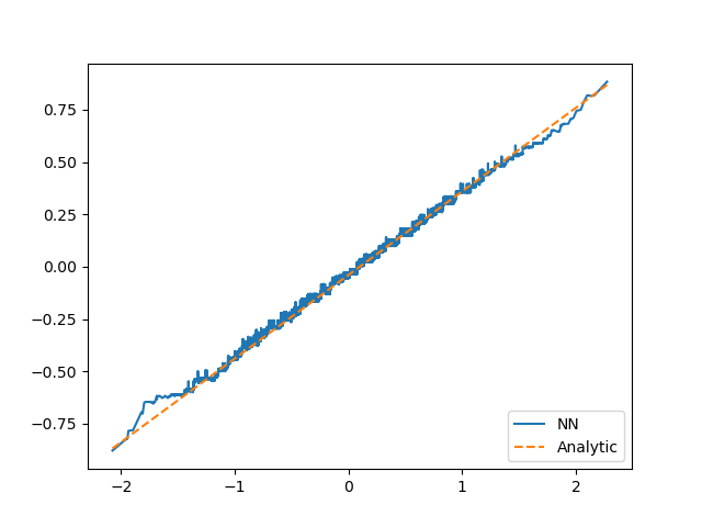
Refer to caption
NT=10subscript𝑁𝑇10N_{T}=10
Refer to caption
NT=20subscript𝑁𝑇20N_{T}=20
Refer to caption
NT=40subscript𝑁𝑇40N_{T}=40
Figure 4: Resolution on [0.5,1]0.51[0.5,1] in dimension N=500𝑁500N=500 : analytic Lions derivatives versus N𝒵𝑁𝒵N{\cal Z} estimated by the network. DeepSet network for 𝒰𝒰{\cal U}, AD-DeepSet for 𝒵𝒵{\cal Z}. ReLU activation function.

As mentioned in Section 4.3, in theory, the proposed methodology should learn the solution for any initial law μ0subscript𝜇0\mu_{0} in the space of measures so that we should be able to solve the problem in infinite dimension. We test our algorithm by sampling μ0subscript𝜇0\mu_{0} in the following way: for a sample j𝑗j, we pick up a mean M^[1,1]^𝑀11\hat{M}\in[-1,1] and a standard deviation σ[0.2,1]𝜎0.21\sigma\in[0.2,1] with an uniform law. Then X0i,j𝒩(M^,σ2)i=1,,Nformulae-sequencesimilar-tosubscriptsuperscript𝑋𝑖𝑗0𝒩^𝑀superscript𝜎2𝑖1𝑁X^{i,j}_{0}\sim{\cal N}(\hat{M},\sigma^{2})\;\;\;i=1,\ldots,N and as before we use the forward process:

Xk+1i,jsuperscriptsubscript𝑋𝑘1𝑖𝑗\displaystyle X_{k+1}^{i,j} =Xki,j+σΔWki,j,k=0,,NT1,i=1,,N.formulae-sequenceabsentsuperscriptsubscript𝑋𝑘𝑖𝑗𝜎Δsuperscriptsubscript𝑊𝑘𝑖𝑗formulae-sequence𝑘0subscript𝑁𝑇1𝑖1𝑁\displaystyle=\;X_{k}^{i,j}+\sigma\Delta W_{k}^{i,j},\;\;k=0,\ldots,N_{T}-1,\;\;\;i=1,\ldots,N. (5.15)

After the training part, we try to recover the initial solution and the initial Lions derivative for a given μ0subscript𝜇0\mu_{0} following a gaussian law. Results are given on figure 5. The Lions derivative is relatively correctly calculated but the initial value can get an error around 15%percent1515\%.

Refer to caption
Solution for μ0=𝒩(0.8,0.09)subscript𝜇0𝒩0.80.09\mu_{0}={\cal N}(-0.8,0.09)
Refer to caption
Lions derivative for μ0=𝒩(0.8,0.09)subscript𝜇0𝒩0.80.09\mu_{0}={\cal N}(-0.8,0.09)
Refer to caption
Solution for μ0=𝒩(0.,0.36)\mu_{0}={\cal N}(0.,0.36)
Refer to caption
Lions derivative for μ0=𝒩(0.,0.36)\mu_{0}={\cal N}(0.,0.36)
Refer to caption
Solution for μ0=𝒩(0.8,0.81)subscript𝜇0𝒩0.80.81\mu_{0}={\cal N}(0.8,0.81)
Refer to caption
Lions derivative for μ0=𝒩(0.8,0.81)subscript𝜇0𝒩0.80.81\mu_{0}={\cal N}(0.8,0.81)
Figure 5: Solution and Lions derivative after a single training, with N=500𝑁500N=500, NT=30subscript𝑁𝑇30N_{T}=30, with ReLU activation function, a single DeepSet network for 𝒰𝒰{\cal U} which is differentiated to approximate 𝒵𝒵{\cal Z}. For the solution, the x𝑥x-axis corresponds to the sample number and the y𝑦y-axis is the value of the estimated solution. For the Lions derivative, the x𝑥x-axis is the state space and the y𝑦y-axis is the value of the derivative.

More generally, if we want to solve the PDE at each time step in the Wasserstein space, we can use Algorithm 3. In order to illustrate the exploration of the Wasserstein space we plot in Figure 6 the graphs of (Xi,N𝒵^(𝑿,Xi))superscript𝑋𝑖𝑁^𝒵𝑿superscript𝑋𝑖(X^{i},N\hat{\cal Z}({\boldsymbol{X}},X^{i})), i𝑖i == 1,,N,1𝑁1,\ldots,N, vs Xisuperscript𝑋𝑖X^{i} maps-to\mapsto μv(t,Xi)(Xi)subscript𝜇𝑣𝑡subscriptsuperscript𝑋𝑖superscript𝑋𝑖\partial_{\mu}v(t,\mathbb{P}_{X^{i}})(X^{i}), when Xtisuperscriptsubscript𝑋𝑡𝑖X_{t}^{i} leads-to\leadsto random mixture of Gaussian laws, for N𝑁N == 300300300, NTsubscript𝑁𝑇N_{T} == 303030. We observe that we are able to estimate correctly the Lions derivative of the solution (and therefore the optimal control) on several probability measures through a randomized training. Concerning the solution itself, we observe similar behavior as in Figure 5 with an error of order 10-15% so we do not show the plots. Further numerical studies are left to future research to improve the estimation of the solution with the randomization procedure.
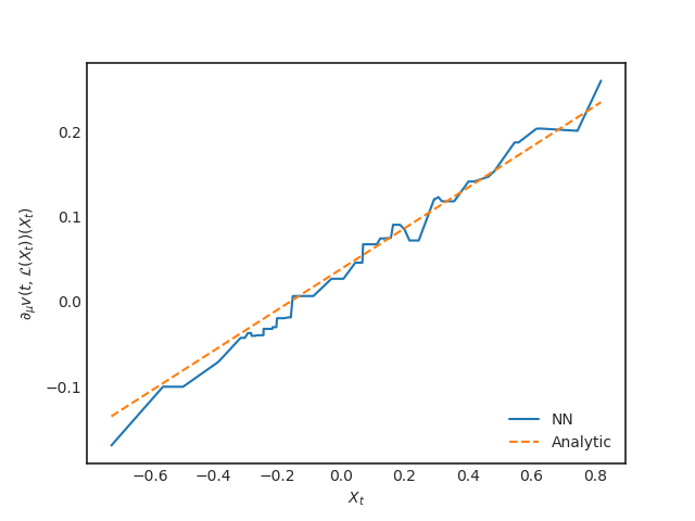
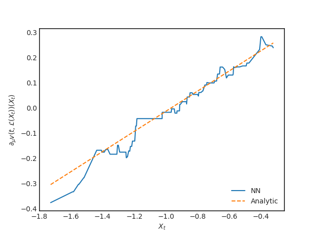
Refer to caption
t=0.2𝑡0.2t=0.2
Refer to caption
t=0.5𝑡0.5t=0.5
Refer to caption
t=0.7𝑡0.7t=0.7
Figure 6: Analytic Lions derivative versus N𝒵𝑁𝒵N{\cal Z} estimated by the network. Dimension N=300𝑁300N=300, number of time steps NT=30subscript𝑁𝑇30N_{T}=30. We use a DeepSet network for 𝒰𝒰{\cal U} with ReLU activation functions, and 𝒵𝒵{\cal Z} its automatic derivative.

5.3 Mean-variance problem

We consider the celebrated Markowitz portfolio selection problem where an investor can invest at any time t𝑡t an amount αtsubscript𝛼𝑡\alpha_{t} in a risky asset (assumed for simplicity to follow a Black-Scholes model with constant rate of return β𝛽\beta and volatility ν𝜈\nu >> 00), hence generating a wealth process X𝑋X == Xαsuperscript𝑋𝛼X^{\alpha} with dynamics

dXt𝑑subscript𝑋𝑡\displaystyle dX_{t} =αtβdt+αtνdWt,0tT,X0=x0.formulae-sequenceformulae-sequenceabsentsubscript𝛼𝑡𝛽𝑑𝑡subscript𝛼𝑡𝜈𝑑subscript𝑊𝑡0𝑡𝑇subscript𝑋0subscript𝑥0\displaystyle=\;\alpha_{t}\beta dt+\alpha_{t}\nu dW_{t},\quad 0\leq t\leq T,\;X_{0}=x_{0}\in\operatorname{\mathbb{R}}.

The goal is then to minimize over portfolio control α𝛼\alpha the mean-variance criterion:

J(α)𝐽𝛼\displaystyle J(\alpha) =λVar(XTα)𝔼[XTα],absent𝜆Varsuperscriptsubscript𝑋𝑇𝛼𝔼delimited-[]superscriptsubscript𝑋𝑇𝛼\displaystyle=\;\lambda{\rm Var}(X_{T}^{\alpha})-\mathbb{E}[X_{T}^{\alpha}],

where λ𝜆\lambda >> 00 is a parameter related to the risk aversion of the investor. Due to the presence of the variance term VarVar{\rm Var} in the criterion, the Markowitz problem falls into the class of McKean-Vlasov control problems, and the associated value function v𝑣v satisfies the Bellman equation (2.5) on [0,T]×𝒫2()0𝑇subscript𝒫2[0,T]\times{\cal P}_{2}(\operatorname{\mathbb{R}}) with r𝑟r == 00, σ0subscript𝜎0\sigma_{0} \equiv 00,

{h(x,μ,z,γ)=infa[zaβ+12γa2ν2]=R2z2γ,z,γ>0,𝒢(μ)=λ𝔼μ|ξ𝔼μ[ξ]|2𝔼μ[ξ],μ𝒫2(),casesformulae-sequence𝑥𝜇𝑧𝛾subscriptinfimum𝑎delimited-[]𝑧𝑎𝛽12𝛾superscript𝑎2superscript𝜈2𝑅2superscript𝑧2𝛾formulae-sequence𝑧𝛾0otherwiseformulae-sequence𝒢𝜇𝜆subscript𝔼𝜇superscript𝜉subscript𝔼𝜇delimited-[]𝜉2subscript𝔼𝜇delimited-[]𝜉𝜇subscript𝒫2otherwise\begin{cases}h(x,\mu,z,\gamma)\;=\;\inf_{a\in\operatorname{\mathbb{R}}}\big{[}za\beta+\frac{1}{2}\gamma a^{2}\nu^{2}\big{]}\;=\;-\frac{R}{2}\frac{z^{2}}{\gamma},\quad z\in\operatorname{\mathbb{R}},\gamma>0,\\ {\cal G}(\mu)\;=\;\lambda\mathbb{E}_{\mu}\big{|}\xi-\mathbb{E}_{\mu}[\xi]\big{|}^{2}-\mathbb{E}_{\mu}[\xi],\quad\mu\in{\cal P}_{2}(\operatorname{\mathbb{R}}),\end{cases} (5.16)

where we set R𝑅R :=assign:= β2/ν2superscript𝛽2superscript𝜈2\beta^{2}/\nu^{2}.

The associated finite-dimensional PDE with N𝑁N particles is given by

{tvNR2i=1N(DxivN)2Dxi2vN=0,t[0,T),𝒙=(x1,,xN)(d)N,vN(T,𝒙)=𝒢(μ¯(𝒙)).casesformulae-sequencesubscript𝑡superscript𝑣𝑁𝑅2superscriptsubscript𝑖1𝑁superscriptsubscript𝐷subscript𝑥𝑖superscript𝑣𝑁2superscriptsubscript𝐷subscript𝑥𝑖2superscript𝑣𝑁0formulae-sequence𝑡0𝑇𝒙subscript𝑥1subscript𝑥𝑁superscriptsuperscript𝑑𝑁otherwisesuperscript𝑣𝑁𝑇𝒙𝒢¯𝜇𝒙otherwise\begin{cases}\partial_{t}v^{N}-\frac{R}{2}\displaystyle\sum_{i=1}^{N}\frac{(D_{x_{i}}v^{N})^{2}}{D_{x_{i}}^{2}v^{N}}=0,\quad t\in[0,T),{\boldsymbol{x}}=(x_{1},\ldots,x_{N})\in(\operatorname{\mathbb{R}}^{d})^{N},\\ v^{N}(T,{\boldsymbol{x}})\;=\;{\cal G}(\bar{\mu}({\boldsymbol{x}})).\end{cases} (5.17)

We refer to [IP19] for the McKean-Vlasov approach to Markowitz mean-variance problems (in a more general context), and we recall that the solution to the Bellman equation is given by

v(t,μ)=λeR(Tt)𝔼μ|ξ𝔼μ[ξ]|2𝔼μ[ξ]14λ[eR(Tt)1]𝑣𝑡𝜇𝜆superscript𝑒𝑅𝑇𝑡subscript𝔼𝜇superscript𝜉subscript𝔼𝜇delimited-[]𝜉2subscript𝔼𝜇delimited-[]𝜉14𝜆delimited-[]superscript𝑒𝑅𝑇𝑡1\displaystyle v(t,\mu)=\;\lambda e^{-R(T-t)}\mathbb{E}_{\mu}\big{|}\xi-\mathbb{E}_{\mu}[\xi]\big{|}^{2}-\mathbb{E}_{\mu}[\xi]-\frac{1}{4\lambda}\big{[}e^{R(T-t)}-1\big{]} (5.18)
μv(t,μ)(x)= 2λeR(Tt)(x𝔼μ[ξ])1,xμv(t,μ)(x)= 2λeR(Tt)formulae-sequencesubscript𝜇𝑣𝑡𝜇𝑥2𝜆superscript𝑒𝑅𝑇𝑡𝑥subscript𝔼𝜇delimited-[]𝜉1subscript𝑥subscript𝜇𝑣𝑡𝜇𝑥2𝜆superscript𝑒𝑅𝑇𝑡\displaystyle\partial_{\mu}v(t,\mu)(x)=\;2\lambda e^{-R(T-t)}(x-\mathbb{E}_{\mu}[\xi])-1,\quad\partial_{x}\partial_{\mu}v(t,\mu)(x)=\;2\lambda e^{-R(T-t)} (5.19)

and in particular V0subscript𝑉0V_{0} :=assign:= infαJ(α)subscriptinfimum𝛼𝐽𝛼\inf_{\alpha}J(\alpha) == v(0,δx0)𝑣0subscript𝛿subscript𝑥0v(0,\delta_{x_{0}}) == x014λ[eRT1]subscript𝑥014𝜆delimited-[]superscript𝑒𝑅𝑇1-x_{0}-\frac{1}{4\lambda}[e^{RT}-1]. Moreover, the optimal portfolio strategy is given by

αt=a^(t,Xt,𝔼[Xt])superscriptsubscript𝛼𝑡^𝑎𝑡superscriptsubscript𝑋𝑡𝔼delimited-[]superscriptsubscript𝑋𝑡\displaystyle\alpha_{t}^{*}\;=\;\hat{a}(t,X_{t}^{*},\mathbb{E}[X_{t}^{*}]) :=βν2[Xt𝔼[Xt]eR(Tt)2λ]assignabsent𝛽superscript𝜈2delimited-[]superscriptsubscript𝑋𝑡𝔼delimited-[]superscriptsubscript𝑋𝑡superscript𝑒𝑅𝑇𝑡2𝜆\displaystyle:=\;-\frac{\beta}{\nu^{2}}\Big{[}X_{t}^{*}-\mathbb{E}[X_{t}^{*}]-\frac{e^{R(T-t)}}{2\lambda}\Big{]} (5.20)
=βν2[Xtx0eRT2λ],0tT,formulae-sequenceabsent𝛽superscript𝜈2delimited-[]superscriptsubscript𝑋𝑡subscript𝑥0superscript𝑒𝑅𝑇2𝜆0𝑡𝑇\displaystyle=\;-\frac{\beta}{\nu^{2}}\Big{[}X_{t}^{*}-x_{0}-\frac{e^{RT}}{2\lambda}\Big{]},\quad 0\leq t\leq T, (5.21)

where Xsuperscript𝑋X^{*} == Xαsuperscript𝑋superscript𝛼X^{\alpha^{*}} is the optimal wealth process.

We test our Algorithm 2 described in Section 4.2 with the training of the forward process

Xk+1i,N,πsuperscriptsubscript𝑋𝑘1𝑖𝑁𝜋\displaystyle X_{k+1}^{i,N,\pi} =Xki,N,π+R2λΔtk+R2λΔWki,X0i=x0,k=0,,NT1,i=1,,N,formulae-sequenceabsentsuperscriptsubscript𝑋𝑘𝑖𝑁𝜋𝑅2𝜆Δsubscript𝑡𝑘𝑅2𝜆Δsuperscriptsubscript𝑊𝑘𝑖formulae-sequencesuperscriptsubscript𝑋0𝑖subscript𝑥0formulae-sequence𝑘0subscript𝑁𝑇1𝑖1𝑁\displaystyle=\;X_{k}^{i,N,\pi}+\frac{R}{2\lambda}\Delta t_{k}+\frac{\sqrt{R}}{2\lambda}\Delta W_{k}^{i},\quad X_{0}^{i}=x_{0},\;\;k=0,\ldots,N_{T}-1,\;\;\;i=1,\ldots,N, (5.22)

which is the time discretization of the wealth process for a constant portfolio strategy αtsubscript𝛼𝑡\alpha_{t} == β/(2ν2λ)𝛽2superscript𝜈2𝜆\beta/(2\nu^{2}\lambda), which is known to be optimal for the exponential utility function U(x)𝑈𝑥U(x) == e2λxsuperscript𝑒2𝜆𝑥-e^{-2\lambda x}. This corresponds to the choice of bisubscript𝑏𝑖b_{i} == R/(2λ)𝑅2𝜆R/(2\lambda) and σijsubscript𝜎𝑖𝑗\sigma_{ij} == R/(2λ)𝑅2𝜆\sqrt{R}/(2\lambda). Here, notice that μG(μ)(x)subscript𝜇𝐺𝜇𝑥\partial_{\mu}G(\mu)(x) == 2λ(x𝔼μ[ξ])12𝜆𝑥subscript𝔼𝜇delimited-[]𝜉12\lambda(x-\mathbb{E}_{\mu}[\xi])-1, and we then use for the initialization at terminal step NTsubscript𝑁𝑇N_{T}, the DeepDerSet function 𝒵NT((xi)i,x)subscript𝒵subscript𝑁𝑇subscriptsubscript𝑥𝑖𝑖𝑥{\cal Z}_{N_{T}}((x_{i})_{i},x) == 2λ(x1Nixi)12𝜆𝑥1𝑁subscript𝑖subscript𝑥𝑖12\lambda\big{(}x-\frac{1}{N}\sum_{i}x_{i}\big{)}-1 (corresponding to the average function 𝔰((xi)i)𝔰subscriptsubscript𝑥𝑖𝑖\mathfrak{s}((x_{i})_{i}) == 1Nixi1𝑁subscript𝑖subscript𝑥𝑖\frac{1}{N}\sum_{i}x_{i}), which yields the automatic differentiation D𝒵NT((xi)i,x)Dsubscript𝒵subscript𝑁𝑇subscriptsubscript𝑥𝑖𝑖𝑥{\rm D}{\cal Z}_{N_{T}}((x_{i})_{i},x) == 2λ(11N)2𝜆11𝑁2\lambda(1-\frac{1}{N}).

We choose the parameters β=0.15𝛽0.15\beta=0.15, ν=0.35𝜈0.35\nu=0.35, λ=1𝜆1\lambda=1, and the quantile at 99.9%percent99.999.9\% for the truncation in scheme [PWG21], and report the results in Table 11. The optimization parameters are the same as in the semi linear case, except the batch size taken equal to 505050 and the number of gradient iterations after first step taken equal to 400040004000. We use a ReLU Deepset for 𝒰𝒰{\cal U} and a AD-Deepset with a tanh activation function for 𝒵𝒵{\cal Z}. Remark that in this case it is not possible to use a ReLU activation function for the second network.

NTsubscript𝑁𝑇N_{T} Dimension N𝑁N Averaged Std Relative error
10 10 -1.0561 0.001 0.005
10 100 -1.0522 0.0008 0.0017
20 10 -1.0570 0.0008 0.006
20 100 -1.0520 0.0007 0.0015
30 10 -1.0578 0.0011 0.007
30 100 -1.0535 0.0021 0.0029
Table 11: Estimate of 𝔼[vN(0,X01,,X0N)]𝔼delimited-[]superscript𝑣𝑁0superscriptsubscript𝑋01superscriptsubscript𝑋0𝑁\mathbb{E}\big{[}v^{N}(0,X_{0}^{1},\ldots,X_{0}^{N})\big{]} with a deterministic initial condition X0=1,T=1,σ=1formulae-sequencesubscript𝑋01formulae-sequence𝑇1𝜎1X_{0}=1,\ T=1,\ \sigma=1. Average and standard deviation observed over 10 independent runs are reported. The theoretical solution is 1.05040581.0504058-1.0504058 when N,NT+𝑁subscript𝑁𝑇N,N_{T}\rightarrow+\infty.

Moreover, we test the accuracy of the control approximation. We solve the PDE from T/2𝑇2T/2 to T𝑇T starting with the optimal distribution of the wealth at T/2𝑇2T/2, which is given by:

log(XT2η(T/2)x0eRT2λ)subscript𝑋𝑇2𝜂𝑇2subscript𝑥0superscript𝑒𝑅𝑇2𝜆\displaystyle\log\Big{(}\frac{X_{\frac{T}{2}}}{\eta(T/2)}-x_{0}-e^{\frac{RT}{2\lambda}}\Big{)} 𝒩(0,κ(T/2)),similar-toabsent𝒩0𝜅𝑇2\displaystyle\sim\;\mathcal{N}(0,\kappa(T/2)), (5.23)

with

η(t)𝜂𝑡\displaystyle\eta(t) =eR(Tt)2λ,κ2(t)=log(eR(Tt)(eRTeR(Tt))4λ2η(t)2+1),formulae-sequenceabsentsuperscript𝑒𝑅𝑇𝑡2𝜆superscript𝜅2𝑡superscript𝑒𝑅𝑇𝑡superscript𝑒𝑅𝑇superscript𝑒𝑅𝑇𝑡4superscript𝜆2𝜂superscript𝑡21\displaystyle=\;-e^{\frac{R(T-t)}{2\lambda}},\quad\kappa^{2}(t)\;=\;\log\Big{(}\frac{e^{R(T-t)}(e^{RT}-e^{R(T-t)})}{4\lambda^{2}\eta(t)^{2}}+1\Big{)}, (5.24)

and we calculate the solution obtained at date T/2𝑇2T/2 and the control obtained solving the PDE (5.17) that we can compare to the analytical solution given by (5.18) and (5.21). After training, using ns=50subscript𝑛𝑠50n_{s}=50 samples of X(N)ns𝑋superscriptsuperscript𝑁subscript𝑛𝑠X\in(\operatorname{\mathbb{R}}^{N})^{n_{s}} following the law of XT2subscript𝑋𝑇2X_{\frac{T}{2}}, we calculate the control obtained for each sample in each of the dimension. After sorting X𝑋X in a one dimensional array, We plot the result obtained on Figures 78. For the solution, the x𝑥x-axis corresponds to the sample number and the y𝑦y-axis is the value of the estimated solution. For the other plots, the x𝑥x-axis is the state space and the y𝑦y-axis is the value of the corresponding function.
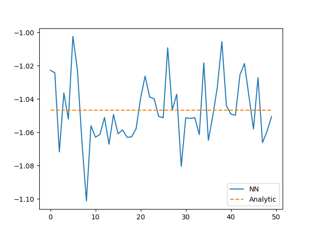
Refer to caption
Solution
Refer to caption
Control
Refer to caption
Derivative
Refer to caption
Second order derivative
Figure 7: Solution and control obtained on the mean variance case at T2𝑇2\frac{T}{2} in dimension 100100100 with 202020 time steps comparing analytic solution to the calculated one (NN). Truncation factor equal to 0.9990.9990.999.
Refer to caption
Solution
Refer to caption
Control
Refer to caption
Derivative
Refer to caption
Second order derivative
Figure 8: Solution and control obtained on the mean variance case at T2𝑇2\frac{T}{2} in dimension 300300300 with 202020 time steps comparing analytic solution to the calculated one (NN). Truncation factor: 0.9990.9990.999.

5.4 A min/max Linear quadratic mean-field control problem

We consider a mean-field model in which the dynamics is linear and the running cost is quadratic in the position, the control and the expectation of the position. The terminal cost is encourages to be close to one of two targets. This type of model is inspired by the min-LQG problem of [SMLN15]. More precisely, we consider the following controlled McKean-Vlasov dynamics

dXtdsubscript𝑋𝑡\displaystyle\mathrm{d}X_{t} =[AXt+A¯𝔼[Xt]+Bαt]dt+σdWt,X0μ0,formulae-sequenceabsentdelimited-[]𝐴subscript𝑋𝑡¯𝐴𝔼delimited-[]subscript𝑋𝑡𝐵subscript𝛼𝑡d𝑡𝜎dsubscript𝑊𝑡similar-tosubscript𝑋0subscript𝜇0\displaystyle=\;\big{[}AX_{t}+\bar{A}\mathbb{E}[X_{t}]+B\alpha_{t}\big{]}\ \mathrm{d}t+\sigma\ \mathrm{d}W_{t},\quad X_{0}\sim\mu_{0}, (5.25)

where α𝛼\alpha == (αt)tsubscriptsubscript𝛼𝑡𝑡(\alpha_{t})_{t} is the control, and the agent aims to minimize the functional cost

J(α)=𝔼[0Tf(Xt,𝔼[Xt],αt)dt+g(XT)]𝐽𝛼𝔼delimited-[]superscriptsubscript0𝑇𝑓subscript𝑋𝑡𝔼delimited-[]subscript𝑋𝑡subscript𝛼𝑡differential-d𝑡𝑔subscript𝑋𝑇\displaystyle J(\alpha)\;=\;\mathbb{E}\Big{[}\int_{0}^{T}f(X_{t},\mathbb{E}[X_{t}],\alpha_{t})\ \mathrm{d}t+g(X_{T})\Big{]} V0=infαJ(α),subscript𝑉0subscriptinfimum𝛼𝐽𝛼\displaystyle\;\rightarrow\quad V_{0}\;=\;\inf_{\alpha}J(\alpha), (5.26)

where the running and terminal costs are given by

f(x,x¯,a)=12(Qx2+Q¯(xSx¯)2+Ra2),𝑓𝑥¯𝑥𝑎12𝑄superscript𝑥2¯𝑄superscript𝑥𝑆¯𝑥2𝑅superscript𝑎2\displaystyle f(x,\bar{x},a)\;=\;\frac{1}{2}\left(Qx^{2}+\bar{Q}(x-S\bar{x})^{2}+Ra^{2}\right), g(x)=min{|xξ1|2,|xξ2|2},𝑔𝑥superscript𝑥subscript𝜉12superscript𝑥subscript𝜉22\displaystyle\quad g(x)\;=\;\min\left\{|x-\xi_{1}|^{2},|x-\xi_{2}|^{2}\right\}, (5.27)

for some non-negative constants Q𝑄Q, Q¯¯𝑄\bar{Q}, S𝑆S, R𝑅R, and two real numbers ξ1subscript𝜉1\xi_{1} and ξ2subscript𝜉2\xi_{2}.

The value function to the mean-field type control problem (5.26) is solution to the Bellman (semi-linear PDE) equation (2.5) with r𝑟r == 00, and

h(x,μ,z,γ)𝑥𝜇𝑧𝛾\displaystyle h(x,\mu,z,\gamma) =infa{[Ax+A¯𝔼μ[ξ]+Ba]z+12(Qx2+Q¯(xS𝔼μ[ξ])2+Ra2)}+σ22γabsentsubscriptinfimum𝑎delimited-[]𝐴𝑥¯𝐴subscript𝔼𝜇delimited-[]𝜉𝐵𝑎𝑧12𝑄superscript𝑥2¯𝑄superscript𝑥𝑆subscript𝔼𝜇delimited-[]𝜉2𝑅superscript𝑎2superscript𝜎22𝛾\displaystyle=\;\inf_{a\in\operatorname{\mathbb{R}}}\big{\{}\big{[}Ax+\bar{A}\mathbb{E}_{\mu}[\xi]+Ba\big{]}z+\frac{1}{2}\left(Qx^{2}+\bar{Q}(x-S\mathbb{E}_{\mu}[\xi])^{2}+Ra^{2}\right)\big{\}}+\frac{\sigma^{2}}{2}\gamma (5.28)
=[Ax+A¯𝔼μ[ξ]]zB22Rz2+12(Qx2+Q¯(xS𝔼μ[ξ])2)+σ22γ,absentdelimited-[]𝐴𝑥¯𝐴subscript𝔼𝜇delimited-[]𝜉𝑧superscript𝐵22𝑅superscript𝑧212𝑄superscript𝑥2¯𝑄superscript𝑥𝑆subscript𝔼𝜇delimited-[]𝜉2superscript𝜎22𝛾\displaystyle=\;\big{[}Ax+\bar{A}\mathbb{E}_{\mu}[\xi]\big{]}z-\frac{B^{2}}{2R}z^{2}+\frac{1}{2}\left(Qx^{2}+\bar{Q}(x-S\mathbb{E}_{\mu}[\xi])^{2}\right)+\frac{\sigma^{2}}{2}\gamma, (5.29)

where the minimizer in the above infinfimum\inf is given by a=BRz𝑎𝐵𝑅𝑧a=-\frac{B}{R}z, and the terminal condition 𝒢(μ)𝒢𝜇{\cal G}(\mu) == 𝔼μmin{|ξξ1|2,|ξξ2|2}subscript𝔼𝜇superscript𝜉subscript𝜉12superscript𝜉subscript𝜉22\mathbb{E}_{\mu}\min\left\{|\xi-\xi_{1}|^{2},|\xi-\xi_{2}|^{2}\right\} is the expected minimal distance to one of the targets ξ1,ξ2subscript𝜉1subscript𝜉2\xi_{1},\xi_{2}.

For the sake of illustration, we present several test cases.

The targets are at ξ1=0.25subscript𝜉10.25\xi_{1}=0.25 and ξ2=1.75subscript𝜉21.75\xi_{2}=1.75. Here we used A=A¯=0𝐴¯𝐴0A=\bar{A}=0, B=1𝐵1B=1, Q=0,Q¯=S=R=1formulae-sequence𝑄0¯𝑄𝑆𝑅1Q=0,\bar{Q}=S=R=1, and a time horizon T=0.5𝑇0.5T=0.5. The initial distribution μ0subscript𝜇0\mu_{0} is a Gaussian 𝒩(x0,ϑ02)𝒩subscript𝑥0superscriptsubscriptitalic-ϑ02\mathcal{N}(x_{0},\vartheta_{0}^{2}). We consider the following test cases:

  1. 1.

    σ=0.3,x0=1,ϑ0=0.2formulae-sequence𝜎0.3formulae-sequencesubscript𝑥01subscriptitalic-ϑ00.2\sigma=0.3,x_{0}=1,\vartheta_{0}=0.2,

  2. 2.

    σ=0.5,x0=0.625,ϑ0=0.2formulae-sequence𝜎0.5formulae-sequencesubscript𝑥00.625subscriptitalic-ϑ00.2\sigma=0.5,x_{0}=0.625,\vartheta_{0}=\sqrt{0.2},

  3. 3.

    σ=0.3,x0=0.625,ϑ0=0.2formulae-sequence𝜎0.3formulae-sequencesubscript𝑥00.625subscriptitalic-ϑ00.2\sigma=0.3,x_{0}=0.625,\vartheta_{0}=\sqrt{0.2},

  4. 4.

    σ=0.3,x0=0.625,ϑ0=0.4formulae-sequence𝜎0.3formulae-sequencesubscript𝑥00.625subscriptitalic-ϑ00.4\sigma=0.3,x_{0}=0.625,\vartheta_{0}=\sqrt{0.4}.

References are given in table 12: they are calculated by the PDE method in [ACD10] (in the context of mean field games; see [AL15] for the adaptation to the PDE system arising in mean field control) with step size in space and time of size 103superscript10310^{-3}, and the neural network method referred to as Algorithm 1 in [CL19] with N=10000𝑁10000N=10000 and NTsubscript𝑁𝑇N_{T} == 505050.

Case Benchmark Global
1 0.22560.22560.2256 0.2273(0.004)0.22730.0040.2273(0.004)
2 0.20850.20850.2085 0.2098(0.006)0.20980.0060.2098(0.006)
3 0.17340.17340.1734 0.1742(0.005)0.17420.0050.1742(0.005)
4 0.22760.22760.2276 0.2300(0.009)0.23000.0090.2300(0.009)
Table 12: Min-LQC example reference solutions : benchmark solution estimated by finite difference scheme and Algorithm 1 in [CL19] with N𝑁N == 100001000010000, NTsubscript𝑁𝑇N_{T} == 505050, 10 neurons and 3 hidden layers, tanh activation function, average on 10 runs.

In table 13, we give the results obtained with different time discretization and dimension for the DPBD scheme using ReLU activation functions with a DeepSet network for 𝒰𝒰{\cal U} and a second AD-DeepSet network to estimate 𝒵𝒵{\cal Z}. Results are very good except for test case 1 where a small bias appears.

Case N=100,NT=30formulae-sequence𝑁100subscript𝑁𝑇30N=100,N_{T}=30 N=100,NT=60formulae-sequence𝑁100subscript𝑁𝑇60N=100,N_{T}=60 N=500,NT=30formulae-sequence𝑁500subscript𝑁𝑇30N=500,N_{T}=30 N=500,NT=60formulae-sequence𝑁500subscript𝑁𝑇60N=500,N_{T}=60
1 0.2370(0.013)0.23700.0130.2370(0.013) 0.2382(0.012)0.23820.0120.2382(0.012) 0.2446(0.013)0.24460.0130.2446(0.013) 0.2495(0.09)0.24950.090.2495(0.09)
2 0.2088(0.002)0.20880.0020.2088(0.002) 0.2092(0.001)0.20920.0010.2092(0.001) 0.2106(0.003)0.21060.0030.2106(0.003) 0.2105(0.003)0.21050.0030.2105(0.003)
3 0.1774(0.007)0.17740.0070.1774(0.007) 0.1784(0.005)0.17840.0050.1784(0.005) 0.1819(0.005)0.18190.0050.1819(0.005) 0.1785(0.008)0.17850.0080.1785(0.008)
4 0.2279(0.005)0.22790.0050.2279(0.005) 0.2264(0.005)0.22640.0050.2264(0.005) 0.2292(0.006)0.22920.0060.2292(0.006) 0.2274(0.006)0.22740.0060.2274(0.006)
Table 13: Min-LQC example with DPBD scheme using ReLU activation functions with a DeepSet network for 𝒰𝒰{\cal U} and a second AD-DeepSet network to estimate 𝒵𝒵{\cal Z}, average on 10 runs, standard deviation in parenthesis.

In table 14, we give the same results using a single network. Here the results are very good for all test cases. Using two networks, the algorithm certainly face difficulties to approximate the derivatives near maturities which is not required using a single network.

Case N=100,NT=30formulae-sequence𝑁100subscript𝑁𝑇30N=100,N_{T}=30 N=100,NT=60formulae-sequence𝑁100subscript𝑁𝑇60N=100,N_{T}=60 N=500,NT=30formulae-sequence𝑁500subscript𝑁𝑇30N=500,N_{T}=30 N=500,NT=60formulae-sequence𝑁500subscript𝑁𝑇60N=500,N_{T}=60
1 0.2289(0.0006)0.22890.00060.2289(0.0006) 0.2271(0.001)0.22710.0010.2271(0.001) 0.2290(0.0004)0.22900.00040.2290(0.0004) 0.2271(0.0008)0.22710.00080.2271(0.0008)
2 0.2083(0.0008)0.20830.00080.2083(0.0008) 0.2086(0.0007)0.20860.00070.2086(0.0007) 0.2097(0.0008)0.20970.00080.2097(0.0008) 0.2089(0.0004)0.20890.00040.2089(0.0004)
3 0.1740(0.001)0.17400.0010.1740(0.001) 0.1740(0.001)0.17400.0010.1740(0.001) 0.1742(0.0004)0.17420.00040.1742(0.0004) 0.1729(0.0007)0.17290.00070.1729(0.0007)
4 0.2276(0.001)0.22760.0010.2276(0.001) 0.2310(0.003)0.23100.0030.2310(0.003) 0.2282(0.0008)0.22820.00080.2282(0.0008) 0.2278(0.001)0.22780.0010.2278(0.001)
Table 14: Min-LQC example with DBDP scheme using ReLU activation functions and a single DeepSet network for 𝒰𝒰{\cal U} which is differentiated to approximate 𝒵𝒵{\cal Z}, average on 10 run, standard deviation in parenthesis.
Refer to caption
Case 1
Refer to caption
Case 2
Refer to caption
Case 3
Refer to caption
Case 4
Figure 9: Control calculated at t=0𝑡0t=0 for Min-LQC examples: comparison DBDP using a single DeepSet network with NT=50subscript𝑁𝑇50N_{T}=50, N=500𝑁500N=500 and global approximation.

References

  • [ACD10] Y. Achdou and I. Capuzzo-Dolcetta “Mean field games: numerical methods” In SIAM J. Numer. Anal. 48.3, 2010, pp. 1136–1162
  • [AL15] Y. Achdou and M. Laurière “On the system of partial differential equations arising in mean field type control” In Discrete Contin. Dyn. Syst. 35.9, 2015, pp. 3879–3900
  • [Bec+20] C. Beck, M. Hutzenthaler, A. Jentzen and B. Kuckuck “An overview on deep learning-based approximation methods for partial differential equations” In arXiv:2012.12348v1, 2020
  • [BP19] M. Basei and H. Pham “A weak martingale approach to linear-quadratic McKean-Vlasov stochastic control problem” In Journal of Optimization Theory and Applications 181.2, 2019, pp. 347–382
  • [BRT20] B. Bloem-Reddy and Y.W. Teh “Probabilistic symmetries and invariant neural networks” In Journal of Machine Learning Research 21, 2020, pp. 1–61
  • [CD18] R. Carmona and F. Delarue “Probabilistic Theory of Mean Field Games: vol. I, Mean Field FBSDEs, Control, and Games,” Springer, 2018
  • [CD18a] R. Carmona and F. Delarue “Probabilistic Theory of Mean Field Games: vol. II, Mean Field FBSDEs, Control, and Games,” Springer, 2018
  • [CFS15] R. Carmona, J.-P. Fouque and L. Sun “Mean field games and systemic risk” In Commun. Math. Sci. 13.4, 2015, pp. 911–933
  • [CL19] R. Carmona and M. Laurière “Convergence analysis of machine learning algorithms for the numerical solution of mean field control and games: II- the finite horizon case” In arXiv:1908.01613, to appear in The Annals of Applied Probability, 2019
  • [CUH16] D.-A. Clevert, T. Unterthiner and S. Hochreiter “Fast and Accurate Deep Network Learning by Exponential Linear Units (ELUs)” In 4th International Conference on Learning Representations, ICLR 2016, San Juan, Puerto Rico, May 2-4, 2016, Conference Track Proceedings, 2016
  • [CWNMW19] Q. Chan-Wai-Nam, J. Mikael and X. Warin “Machine Learning for Semi Linear PDEs” In Journal of Scientific Computing 79, 2019, pp. 1667–1712
  • [Dje20] F Djete “Extended mean-field control problem: a propagation of chaos result” In arXiv:2006.12996, 2020
  • [EHJ17] W. E, J. Han and A. Jentzen “Deep learning-based numerical methods for high-dimensional parabolic partial differential equations and backward stochastic differential equations” In Communications in Mathematics and Statistics 5.4 Springer, 2017, pp. 349–380
  • [FZ20] J.-P. Fouque and Z. Zhang “Deep Learning Methods for Mean Field Control Problems with Delay” In Frontiers in Applied Mathematics and Statistics 6, 2020
  • [GMS21] W. Gangbo, S. Mayorga and A. Swiech “Finite Dimensional Approximations of Hamilton–Jacobi–Bellman Equations in Spaces of Probability Measures” In SIAM Journal on Mathematical Analysis 53.2, 2021, pp. 1320–1356
  • [GMW19] M. Germain, J. Mikael and X. Warin “Numerical resolution of McKean-Vlasov FBSDEs using neural networks” In arXiv:1909.12678, 2019
  • [GPW22] M. Germain, H. Pham and X. Warin “Convergence analysis of particles approximation of PDEs in Wasserstein space” In arXiv:2103.00837, to appear in Journal of Applied Probability 59.4, 2022
  • [GPW22a] M. Germain, H. Pham and X. Warin “Neural networks based algorithms for stochastic control and PDEs in finance” In arXiv:2101.08068 to appear in Machine Learning And Data Sciences For Financial Markets: A Guide To Contemporary Practices Cambridge University Press, 2022
  • [HCM06] M. Huang, P. Caines and R. Malhamé “Large population stochastic dynamic games: closed-loop McKean-Vlasov systems and the Nash certainty equivalence principle” In Communication in Information and Systems 3, 2006, pp. 221–252
  • [HJW18] J. Han, A. Jentzen and E Weinan “Solving high-dimensional partial differential equations using deep learning” In Proceedings of the National Academy of Sciences 115.34 National Acad Sciences, 2018, pp. 8505–8510
  • [Hor91] K. Hornik “Approximation Capabilities of Multilayer Feedforward Networks” In Neural Networks 4, 1991, pp. 251–257
  • [HPW20] C. Huré, H. Pham and X. Warin “Deep backward schemes for high-dimensional nonlinear PDEs” In Mathematics of Computation 89.324, 2020, pp. 1547–1579
  • [Hut+20] M. Hutzenthaler, A. Jentzen, T. Kruse and T.A. Nguyen “A proof that rectified deep neural networks overcome the curse of dimensionality in the numerical approximation of semilinear heat equation” In SN partial differential equations and applications 1.10, 2020, pp. 1–34
  • [IP19] A. Ismail and H. Pham “Robust Markowitz mean-variance portfolio selection under ambiguous covariance matrix” In Mathematical Finance 29.174-207, 2019
  • [KB14] D. P. Kingma and J. Ba “Adam: A method for stochastic optimization” In arXiv preprint arXiv:1412.6980, 2014
  • [Lab12] P.H. Labordère “Counterparty risk valuation: a marked branching diffusion approach” In Hal-00677348, 2012
  • [Lac17] D. Lacker “Limit theory for controlled McKean-Vlasov dynamics” In SIAM Journal on Control and Optimization 55.3, 2017, pp. 1641–1672
  • [LL07] J.M. Lasry and P.L. Lions “Mean field games” In Japanese Journal of Mathematics 2, 2007, pp. 229–260
  • [PP90] E. Pardoux and S. Peng “Adapted solution of a backward stochastic differential equation” In Systems & Control Letters 14.1 Elsevier, 1990, pp. 55–61
  • [PW17] H. Pham and X. Wei “Dynamic programming for optimal control of stochastic McKean-Vlasov dynamics” In SIAM Journal on Control and Optimization 55.2, 2017, pp. 1069–1101
  • [PWG21] H. Pham, X. Warin and M. Germain “Neural networks-based backward scheme for fully nonlinear PDEs.” In SN Partial Differential Equations and Applications 2.16, 2021
  • [RQ+17] C. R. Qi, H. Su, K. Mo and L. J. Guibas “PointNet: Deep Learning on Point Sets for 3D Classification and Segmentation” In 2017 IEEE Conference on Computer Vision and Pattern Recognition (CVPR), 2017, pp. 77–85
  • [Rut+20] L. Ruthotto, S. J. Osher, W. Li, L. Nurbekyan and S. W. Fung “A machine learning framework for solving high-dimensional mean field game and mean field control problems” In Proc. Natl. Acad. Sci. USA 117.17, 2020, pp. 9183–9193
  • [SMLN15] R. Salhab, R. P. Malhamé and J. Le Ny “A dynamic game model of collective choice in multi-agent systems” In 2015 IEEE 54th Annual Conference on Decision and Control (CDC), 2015, pp. 4444–4449
  • [Smu11] J. Smulevici “On the area of the symmetry orbits of cosmological spacetimes with toroidal or hyperbolic symmetry” In Analysis and PDE 4.2, 2011, pp. 191–245
  • [Wag+19] E. Wagstaff, F. Fuchs, M. Engelcke, I. Posner and M. A. Osborne “On the Limitations of Representing Functions on Sets” 97, Proceedings of Machine Learning Research, 2019, pp. 6487–6494
  • [Wyk08] S. Van Wyk “Partial differential equations and quantum mechanics” In Computer solution in Physics, 2008, pp. 99–139
  • [Zah+17] M. Zaheer, S. Kottur, S. Ravanbakhsh, B. Poczos, R. R Salakhutdinov and A. J Smola “Deep Sets” In Advances in Neural Information Processing Systems 30 Curran Associates, Inc., 2017, pp. 3391–3401