contrastive separative coding for Self-supervised representation learning
Abstract
To extract robust deep representations from long sequential modeling of speech data, we propose a self-supervised learning approach, namely Contrastive Separative Coding (CSC). Our key finding is to learn such representations by separating the target signal from contrastive interfering signals. First, a multi-task separative encoder is built to extract shared separable and discriminative embedding; secondly, we propose a powerful cross-attention mechanism performed over speaker representations across various interfering conditions, allowing the model to focus on and globally aggregate the most critical information to answer the “query” (current bottom-up embedding) while paying less attention to interfering, noisy, or irrelevant parts; lastly, we form a new probabilistic contrastive loss which estimates and maximizes the mutual information between the representations and the global speaker vector. While most prior unsupervised methods have focused on predicting the future, neighboring, or missing samples, we take a different perspective of predicting the interfered samples. Moreover, our contrastive separative loss is free from negative sampling. The experiment demonstrates that our approach can learn useful representations achieving a strong speaker verification performance in adverse conditions.
Index Terms— Speaker verification, speech separation, self attention, contrastive loss
1 Introduction
Learning high-level representations from labeled data has achieved marvelous successes in modern speech processing. To extract reliable speaker representations in realistic situations, however, conventional speaker verification, speaker identification, and speaker diarization (SV, SI, SD) systems generally require complicated pipelines [1, 2, 3]. One has to prepare three independent models: (i) a speech activity detection model to generate short speech segments with no interference or overlapping, (ii) a speaker embedding extraction model, and (iii) a clustering or a PLDA model including covariance matrices is needed to group the short segments to the same or different speaker. Jointly supervised modeling methods[4, 5, 6] have been studied to alleviate the long preparation process and take into account the dependencies between these models. More recently, end-to-end neural speaker diarization [7, 8, 9] has been proposed to overcome the situation that the previous systems can not deal with speaker overlap parts because each time slot is assigned to one speaker.
Despite the breakthrough seen by these supervised methods, many challenges remain, such as data robustness, efficiency, and generalization. To alleviate these issues, improving representation learning requires features that are less specialized towards solving a single supervised task. Unsupervised or self-supervised learning [10, 11, 12, 13, 14] is a promising apparatus towards generic and robust representation learning. A common strategy is to use the conditional dependency between the features of interest and the same shared high-level latent information/context. Advanced work in unsupervised or self-supervised learning has successfully used the strategy to learn deep representations by predicting neighboring or missing words [15, 16], predicting the relative position of image patches [17] or color from grey-scale [18], or most recently predicting future frames [12] or contextual information [11].
Classical predictive coding theories in neuroscience suggest that the brain predicts observations at various levels of abstraction [19, 20]. When one is listening to overlapped speakers, we infer the features of interest conditionally dependent on both low-mid levels of abstraction of the same speaker (e.g., spectrum continuity and structure, timbre, phoneme, syllable, etc.) and high levels of abstraction (E.g., speaker characterizations, spatial position, etc.). Inspired by the above, we hypothesize these different levels of abstraction have shared bottom features. We propose Contrastive Separative Coding (CSC) model as the following: first, an encoder compresses the raw input into a compact latent space of separable and discriminative embedding shared by various levels of abstraction task (Sec.3, 3.3); secondly, we propose a powerful cross-attention model in this latent space to model the high-level abstraction of speaker representations (Sec.3.1); lastly, we form a new probabilistic contrastive loss which estimates and maximizes the mutual information between the representations and the global speaker vector (Sec.3.2).
2 Related Work and our contributions
The compositional attention networks [21] decomposes machine reasoning into a series of attention-based reasoning operations that are directly inferred from the data, without resorting to any strong supervision. Interaction between its two modalities – visual and textual, or knowledge base and query – is mediated through soft-attention only. The soft attention enhances its model’s ability to perform reasoning operations that pertain to the global aggregation of information across different regions of the image. Earlier, cross-stitch strategy [22] has been proposed between text and image, on which both [21] and our proposed cross-attention approach can be regarded as new variations. To the best of our knowledge, however, we are the first to use a cross-attention strategy between high-level speaker representations and low-level speech features.
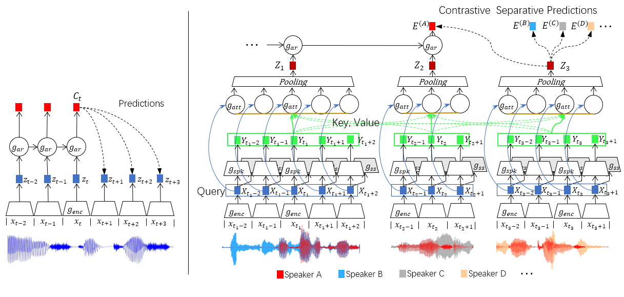
Another closely related prior work that does not resort to any strong supervision is the Contrastive Predictive Coding (CPC) [12], as shown on the left in Fig. 1. Comparing it to our proposed CSC on the right, we summarize our key contributions in four folds:
-
•
While most unsupervised prior work, including [12], has focused on predicting the future, neighboring, or missing samples, our perspective is different in that it focuses on interfered samples, i.e., learning separative representations from observations with various interference.
-
•
To learn mid-level representations by using the powerful cross-attention strategy.
-
•
To study the prediction strategy on latent global speaker features, for the first time at a much higher level of abstraction than the prior work [10, 11, 12, 14, 16]. We consider predicting the “global feature” that spans various observations more interesting, especially across various interfering conditions, thus the model needs to infer more global structure to preserve the latent shared information.
-
•
A novel contrastive separative loss is first used as a bound on mutual information. In contrast to the prior common strategy, our proposed loss models an inverse conditional dependency between the features of interest and the shared high-level latent context, which also holds for estimating the mutual information thanks to its symmetric property. This makes our conditional predictions easier to model and free from negative sampling as generally required in prior work, at the cost of weak supervision about the shared high-level latent context – here is to know the set of mixtures containing signals by the same speaker, e.g., the ones marked in red in Fig. 1.
3 Proposed Approach
On the right of Fig. 1 is the architecture of Contrastive Separative Coding (CSC) model. First, an encoder maps the encoded and segmented input mixture sequences of to sequences of latent representations . We denote them as 2D tensors , where is the feature dimension, is the sequence length. Secondly, task-specific encoders, and , map the shared latent representations to compact latent spaces of various levels of abstraction tasks, i.e., speaker embedding () and speech embedding, respectively. Next, a powerful cross-attention model in the speaker embedding space computes the high-level abstraction of speaker representations that are pooled into . Finally, an autoregressive model summarizes all the past to a global speaker vector .
3.1 Bottom-up Cross Attention
We cast the query vector onto the latent speaker space via the cross-attention model . The bottom-up queries are raised from the shared bottom features X to retrieve the most relevant speaker-dependent global characteristics from the latent speaker space of Y and filter out non-salient, noisy, or redundant information. , , and denote linear transformation functions, where the corresponding input vectors are linearly projected along the feature dimension () into query, key, and value vectors, respectively. Our detailed implementation of these functions is the same as [23].
Specifically, this is achieved by computing the inner product between and :
| (1) |
yielding a cross-attention distribution , where are the sequence lengths of either different observations or the same observation (, amount to self-attention).
Finally, we compute the sum of weighted by the cross-attention distribution , and then average over segments, to produce a separative embedding :
| (2) |
3.2 Contrastive Separative Coding Loss
Next, we introduce CSC loss, which takes the following form:
| (3) | ||||
| (4) |
We denote as the global speaker vector for speaker out of the overall speakers in the training set and the separative embedding for the -th separated signal, for , given that each audio input is a mixture of sources and the -th source is generated by one of the speakers indexed by out of the overall speakers. We assume that the training set sufficiently defined the sample space of their joint distributions. For notational simplicity, we omit the subscript and use to denote , E to denote in the following text, unless otherwise specified. First, we study the relationship between CSC loss and mutual information:
Definition 3.1.
Mutual information of the global speaker vector and the separative embedding is defined as
| (5) |
Then, we make the following assumptions:
Assumption 3.1.
With a suitable mathematical form for function , we can model a density ratio defined as
| (6) |
Assumption 3.2.
Considering the case of , since the separative embedding does not belong to speaker , should not be dependent on . Therefore, it is sensible to assume
| (7) |
Based on these assumptions, we can deduce the claims:
Claim 3.1.
Minimizing CSC loss results in maximizing mutual information between global speaker vector and the separative embedding, since CSC loss serves as an upper bound of the negative mutual information .
Proof.
Next, we study our proposed form of and its associated properties when minimizing CSC loss.
Claim 3.2.
Applying our proposed form of to corresponds to treating each global speaker vector E as a cluster centroid (Gaussian mean) of different separative embedding vectors generated by the same speaker with a learnable parameter controlling the cluster size (Gaussian variance):
| (8) | ||||
| (9) |
Proof.
Considering a density ratio :
Now, we evaluate with the above-defined :
∎
Claim 3.3.
With our proposed form of , minimizing CSC loss results in minimizing the distance between the separative embedding and the corresponding global speaker vector E meanwhile maximizing the distance between other global speaker vectors .
Proof.
By substituting Eq. (4) into Eq. (3), we have
which consists of two terms: (1) the first term is a scaled Euclidean distance with a scalar , which minimizes the Euclidean distance between any global speaker vector and its corresponding separative embedding. (2) the second term is a logarithmic sum of exponentials, with a negative sign on the Euclidean distance, which pulls the separative embedding away from all other global speaker vectors. ∎
Besides, we can also relate the proposed CSC loss with the existing prior work.
Claim 3.4.
CSC loss can be seen as a rescaled -2 normalization of InfoNCE loss proposed in [12].
Proof.
The InfoNCE loss has a different form, than our proposed , we get
∎
3.3 Permutation Invariant Training Speedup
As mentioned in Sec.3, the shared bottom features are jointly learned towards another level of abstraction tasks, i.e., speech separation (SS) to reconstruct the source signals. The joint training loss is , where is the scale-invariant signal-to-noise ratio [24] loss for training , while is for training , where is a regularization loss that avoids collapsing to a trivial solution of all zeros, and is a weighting factor for the joint loss for training . Noted that for computing either the speech loss or the speaker loss in , we need to assign the correct target source. During training, we use the utterance-level permutation invariant training (u-PIT) method [25] to solve the permutation issue. We start with using u-PIT to calculate the speech loss , which expends heavy computation at reconstructing every detail of the signals, while often ignoring the global context. We use the separative embedding to modulate the signal reconstruction in the speech-stimuli space by a FiLM [26] method so that the permutation solution for one task also applies to the other task. We switch to using u-PIT to calculate the speaker loss instead after an empirical number of epochs, thereafter, the speech reconstruction becomes PIT-free and achieves a notable training acceleration.
4 Experiments
4.1 Datasets and Model Setup
We firstly evaluated and compared the embedding learnt by CPC[12] versus our proposed CSC on a small benchmark dataset WSJ0-2mix[27] for a separation task. The separation SDR result by CPC significantly decreased by an absolute dB comparing to CSC, and therefore we continued with CSC to compare with the traditional SV methods on a larger-scale dataset, Libri-2mix, where we split the Librispeech [28] into (1) a training set containing 12055 utterances drawn from 2411 speakers, i.e., utterances per speaker111This limitation makes our corpus much more challenging than the lately released LibriMix [29], meanwhile, more realistic as it was often hard to collect numerous utterances from the user in real industrial applications., (2) a validation set containing another utterances drawn from the same speakers, and (3) a test set containing utterances evenly drawn from speakers.
To built our proposed model CSC, we inherited from DPRNN’s setup [30] for the raw waveform encoding, segmentation, and decoding for the SS task. Then, we used , , and GALR [31] blocks for , , and , respectively. Inherited from the settings in [31, 30], a 5ms (8-sample) window length and were used. We empirically set . For each training epoch, mixture signals of s were generated online by mixing each clean utterance with another random utterance in the training set in a uniform SIR of dB. For testing, mixture signals were pre-mixed in the same SIR range.
For reference systems, we built a SincNet-based SV model [3] SincNet, for it was a conventional speaker-vector-based neural network achieving reproducible and strong performance on Librispeech. Moreover, for the ablation study, we built another reference system CE by using GALR blocks for (note that here could merge into as they no longer had the distinction and that the overall model size kept unchanged for the speaker task) and ablated the proposed method by removing the and models from the graph and replacing the proposed loss with the supervised Cross-Entropy (CE) loss. All the models were implemented and trained using PyTorch.
4.2 Results and Discussion
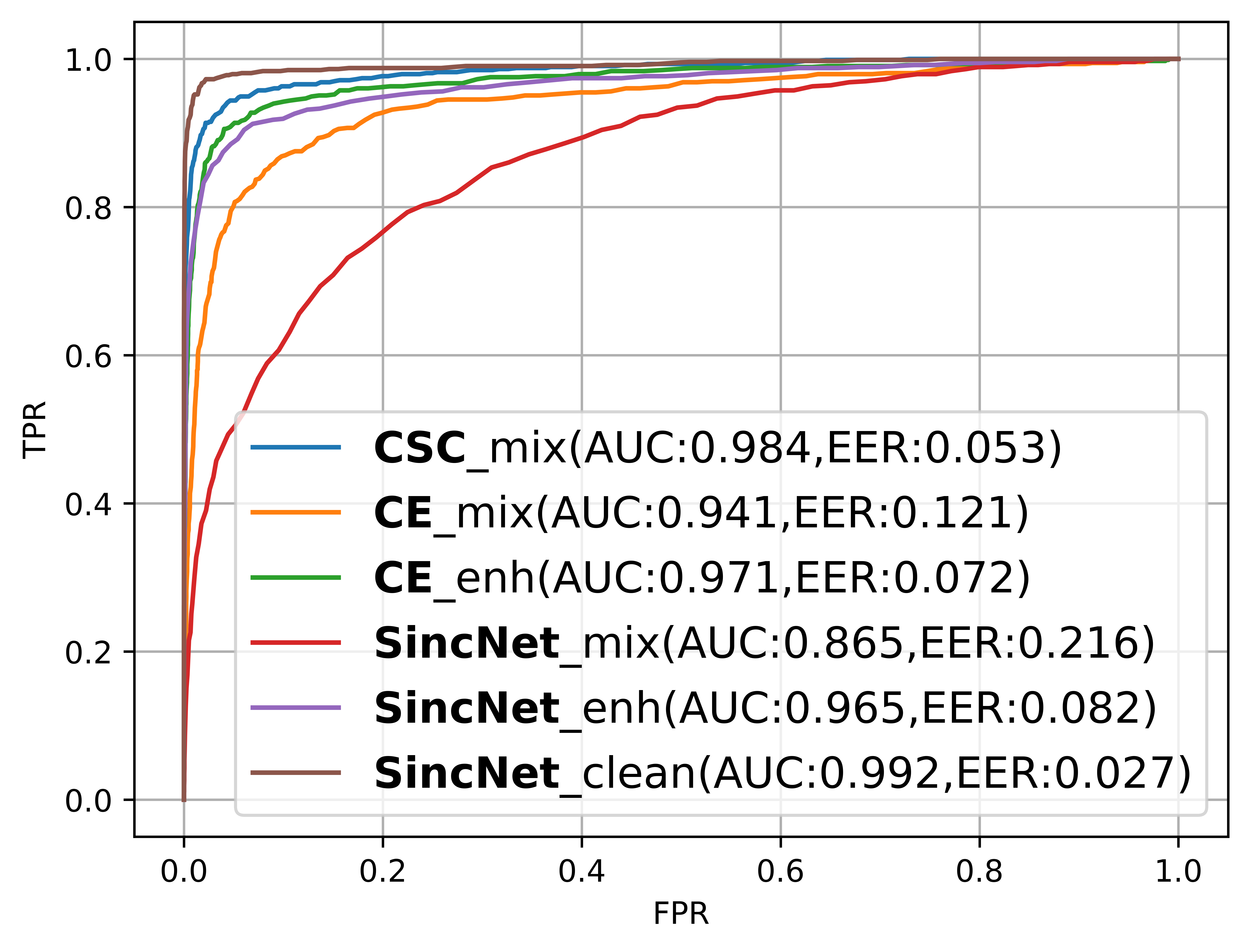
To evaluate the discriminative power of the learned representations, Fig.2(a) shows the Equal Error Rate (EER) and Area Under Curve (AUC) as the performance metrics on the SV task. “[Model]_mix”, “_enh”, and “_clean” indicate systems training and test on mixture data, enhanced/separated data (by pre-processing the mixture using a SOTA SS system [31]), and clean data (which we used as a high-bar reference), respectively. Our proposed system outperforms all reference models by a large margin, suggesting our learned representations have strong discriminative power and can achieve high performance in difficult conditions.
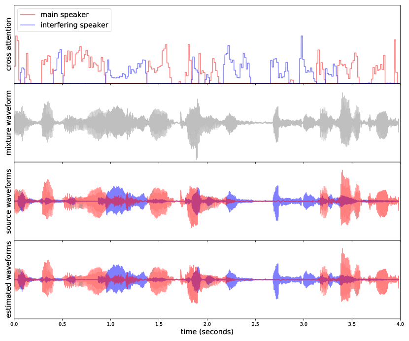
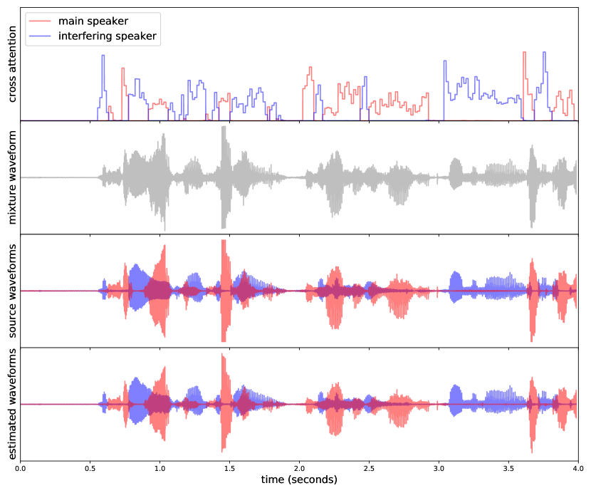
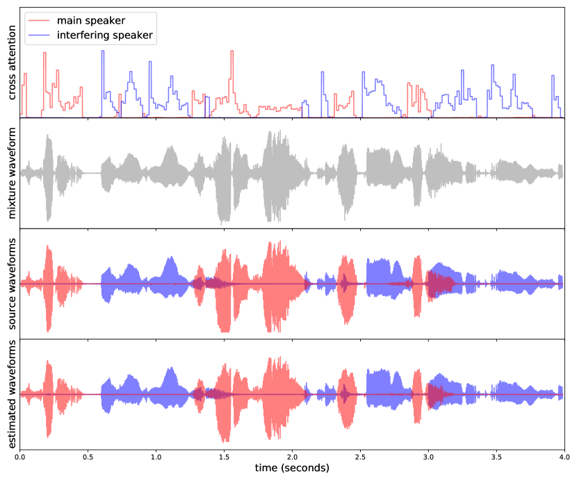
Moreover, as shown in Fig. 2(b)-2(d), the proposed cross-attention mechanism improves the model transparency, since we can easily interpret the attended content, that at any given time segment, it is generally the most salient source in the mixture that triggers the corresponding cross-attention curve. In places where both sources are soft, all cross-attention curves are low to ignore the possibly noisy and unreliable parts. Also, cross-attention curves rarely raise concurrently. These are all surprisingly similar to a human’s auditory selective attention [32, 33, 34, 35] in behavioral and cognitive neurosciences, i.e., a listener can not attend to both two concurrent speech streams, while he usually selects the attended speech and ignores other sounds in a complex auditory scene. Note that this selective cross attention property of our model was automatically learned from the mixture without resorting to any regularization or strong supervision.
5 Conclusions
This paper introduces a novel Contrastive Separative Coding method to draw useful representations directly from observations in complex auditory scenarios. It is helpful to learn low-level shared representations towards various levels of separative task. In-depth theoretical studies are provided on the proposed CSC loss regarding the mutual information estimation and maximization, as well as its connection to the existing prior work. The proposed cross-attention mechanism is shown effective in extracting the global aggregation of information across different corrupted observations in various interfering conditions. The learned representation have strong discriminability that its performance is even approaching the clean-condition performance of a conventional fully-supervised SV system. Another interesting observation is the automatically learned bottom-up cross attentions that are very similar to an auditory selective attention, and we will explore this merit on speaker diarization in our future work.
References
- [1] D. Snyder, D. Garcia-Romero, G. Sell, D. Povey, and S. Khudanpur, “X-vectors: Robust dnn embeddings for speaker recognition,” in ICASSP, 2018, p. 5329–5333.
- [2] Jia Liu Yi Liu, Liang He, “Large margin softmax loss for speaker verification,” in Proc. INTERSPEECH, 2019.
- [3] M. Ravanelli and Y. Bengio, “Speaker recognition from raw waveform with sincnet,” in In Proceedings of SLT 2018, 2018.
- [4] V. S. Narayanaswamy, J. J. Thiagarajan, H. Song, and A. Spanias, “Designing an effective metric learning pipeline for speaker diarization,” in Proc. ICASSP, 2019, p. 5806–5810.
- [5] Z. Huang, S. Watanabe, Y. Fujita, P. Garcia, Y. Shao, D. Povey, and S. Khudanpur, “Speaker diarization with region proposal network,” in ICASSP, 2020.
- [6] V. A. Miasato Filho, D. A. Silva, and L. G. Depra Cuozzo, “Joint discriminative embedding learning, speech activity and overlap detection for the dihard speaker diarization challenge,” in Proc. INTERSPEECH, 2018, p. 2818–2822.
- [7] Y. Fujita, N. Kanda, S. Horiguchi, K. Nagamatsu, and S. Watanabe, “End-to-end neural speaker diarization with permutation-free objectives,” in Proc. INTERSPEECH, 2019.
- [8] Y. Fujita, N. Kanda, S. Horiguchi, Y. Xue, K. Nagamatsu, and S. Watanabe, “End-to-end neural speaker diarization with self-attention,” in arXiv:1909.06247, 2019.
- [9] S. Horiguchi, Y. Fujita, S. Watanabe, Y. Xue, and K. Nagamatsu, “End-to-end speaker diarization for an unknown number of speakers with encoder-decoder based attractors,” in Proc. INTERSPEECH, 2020.
- [10] S. Schneider, A. Baevski, R. Collobert, and M. Auli, “Wav2vec: Unsupervised pre-training for speech recognition,” arXiv preprint arXiv:1904.05862v1, 2019.
- [11] R.D. Hjelm, A. Fedorov, S.L. Marchildon, K. Grewal, P. Bachman, A. Trischler, and Y. Bengio, “Learning deep representations by mutual information estimation and maximization,” in ICLR, 2019.
- [12] A.V.D. Oord, Y. Li, and O. Vinyals, “Representation learning with contrastive predictive coding,” arXiv preprint arXiv:1807.03748, 2018.
- [13] T. Mikolov, I. Sutskever, K. Chen, G. Corrado, and J. Dean, “Distributed representation of words and phrases and their compositionality,” in NIPS, 2013.
- [14] J. Glass Y. Chung, “Speech2vec: a sequence-to-sequence framework for learning word embeddings from speech,” in Interspeech, 2018.
- [15] T. Mikolov, K. Chen, G. Corrado, and J. Dean, “Efficient estimation of word representations in vector space,” arXiv preprint arXiv:1301.3781, 2013.
- [16] Jacob Devlin, Ming-Wei Chang, Kenton Lee, and Kristina Toutanova, “Bert: Pre-training of deep bidirectional transformers for language understanding,” in ACL, 2019, pp. 4171–4186.
- [17] C. Doersch, A. Gupta, and A. A. Efros, “Unsupervised visual representation learning by context prediction,” In ICCV, 2015.
- [18] R. Zhang, P. Isola, and A. A. Efros, “Colorful image colorization,” In European Conference on Computer Vision, p. 649–666, 2016.
- [19] K. Friston, “A theory of cortical responses,” in Philosophical transactions of the Royal Society B: Biological sciences, 2005, p. 360(1456):815–836.
- [20] R. P. Rao and D. H. Ballard, “Predictive coding in the visual cortex: a functional interpretation of some extra-classical receptive-field effects,” in Nature neuroscience, 1999, p. 2(1):79.
- [21] D. A. Hudson and C. D. Manning, “Compositional attention networks for machine reasoning,” in ICLR, 2018.
- [22] Ishan Misra, Abhinav Shrivastava, Abhinav Gupta, and Martial Hebert, “Cross-stitch networks for multi-task learning,” CVPR, 2016.
- [23] Matthias Sperber, Jan Niehues, Graham Neubig, Sebastian Stuker, and Alex Waibel, “Self-attentional acoustic models,” INTERSPEECH, 2018.
- [24] Jonathan Le Roux, Scott Wisdom, Hakan Erdogan, and John R Hershey, “Sdr–half-baked or well done?,” in ICASSP. IEEE, 2019, pp. 626–630.
- [25] Dong Yu, Morten Kolbæk, Zheng-Hua Tan, and Jesper Jensen, “Permutation invariant training of deep models for speaker-independent multi-talker speech separation,” in Proc. ICASSP. IEEE, 2017, pp. 241–245.
- [26] E. Perez, F. Strub, H. Vries, V. Dumoulin, and A. Courville, “Film: Visual reasoning with a general conditioning layer,” in arXiv preprint arXiv:1709.07871, 2017.
- [27] John R Hershey, Zhuo Chen, Jonathan Le Roux, and Shinji Watanabe, “Deep clustering: Discriminative embeddings for segmentation and separation,” in Proc. ICASSP. IEEE, 2016, pp. 31–35.
- [28] Vassil Panayotov, Guoguo Chen, Daniel Povey, and Sanjeev Khudanpur, “Librispeech: an asr corpus based on public domain audio books,” in Proc. ICASSP. IEEE, 2015, pp. 5206–5210.
- [29] J. Cosentino, M. Pariente, S. Cornell, A. Deleforge, and E. Vincent, “Librimix: An open-source dataset for generalizable speech separation,” arXiv preprint arXiv:2005.11262, 2020.
- [30] Yi Luo, Zhuo Chen, and Takuya Yoshioka, “Dual-path rnn: efficient long sequence modeling for time-domain single-channel speech separation,” arXiv preprint arXiv:1910.06379, 2019.
- [31] M. W. Y. Lam, J. Wang, D. Su, and D. Yu, “Effective low-cost time-domain audio separation usingglobally attentive locally recurrent networks,” To appear in SLT2021.
- [32] N. Mesgarani and E. F. Chang, “Selective cortical representation of attended speaker in multi-talker speech perception,” Nature, vol. 485, no. 7397, pp. 233–236, 2012.
- [33] D. S. Costa, V. D. W. Zwaag, L. M. Miller, S. Clarke, and M.Saenz, “Tuning in to sound: frequency-selective attentional filter in human primary auditory cortex,” Journal of Neuroscience, vol. 33, no. 5, pp. 1858–1863, 2013.
- [34] S. J. Lim, M. Wostmann, and J. Obleser, “Selective attention to auditory memory neurally enhances perceptual precision,” Journal of Neuroscience, vol. 35, no. 49, pp. 16094–16104, 2015.
- [35] J. A. O’sullivan, A. J. Power, N. Mesgarani, S. Rajaram, J. J. Foxe, B. G. Shinn-Cunningham, M. Slaney, S. A. Shamma, and E. C. Lalor, “Attentional selection in a cocktail party environment can be decoded from single-trial eeg,” Cerebral Cortex, vol. 25, no. 7, pp. 1697–1706, 2015.