Enhancement for Robustness of Koopman Operator-based
Data-driven Mobile Robotic Systems

Abstract

Koopman operator theory has served as the basis to extract dynamics for nonlinear system modeling and control across settings, including non-holonomic mobile robot control. There is a growing interest in research to derive robustness (and/or safety) guarantees for systems the dynamics of which are extracted via the Koopman operator. In this paper, we propose a way to quantify the prediction error because of noisy measurements when the Koopman operator is approximated via Extended Dynamic Mode Decomposition. We further develop an enhanced robot control strategy to endow robustness to a class of data-driven (robotic) systems that rely on Koopman operator theory, and we show how part of the strategy can happen offline in an effort to make our algorithm capable of real-time implementation. We perform a parametric study to evaluate the (theoretical) performance of the algorithm using a Van der Pol oscillator, and conduct a series of simulated experiments in Gazebo using a non-holonomic wheeled robot.

I Introduction

Employing models for mobile robot motion planning and control can be beneficial for integrating motion constraints in planning [1, 2] and deriving control performance guarantees (e.g., robustness guarantees [3, 4]). Yet, there exist many instances in which robots interact physically with their environment and that these interactions are uncertain. Examples include robots operating in partially-known dynamic environments [5]; legged robots traversing non-smooth terrains [6, 7]; quadrotors flying under the influence of uncertain aerodynamic effects [8, 9, 10, 11]; underwater robots affected by uncertain ocean currents [12]; and steerable needles interacting with soft tissue [13]. Thus, employing pre-selected models may restrict the capability to predict actual robot behaviors when operating under uncertainty [14, 15, 16, 17].

A different way to address uncertainties in robot-environment interactions is by extracting dynamics from data. Multiple distinct approaches have been proposed—including stochastic model extension [17], (deep) reinforcement learning [18], (deep) neural networks [19, 20], and spectral methods [21], to name a few—and deployed in robotics (e.g., [17, 22, 23, 24, 25, 11]). The advent of data-driven methods for modeling complex dynamical systems creates a need for theoretical safety and/or performance guarantees.

Deriving guarantees for methods that rely on extracting dynamics from data for mobile robots is a rapidly-growing focus area [26]. Several efforts focus on cases that involve deep neural networks, e.g., by developing spectrally-normalized margin bounds [27] or by embedding and/or extending Lyapunov stability theory in neural network-based systems for safety (e.g., [28, 29, 30, 31, 32]). Despite their high expressiveness, neural network-based systems continue to require large training data sets, and might lead to instability and unpredictable outputs because of overfitting.

Besides (deep) neural networks, dimensionality reduction and spectral approaches play an important role in data-driven algorithms [21]. Methods like Proper Orthogonal Decomposition [33, 34]), Dynamic Mode Decomposition (DMD) [35] and Extended DMD (EDMD) [36], and their various extensions [37, 38, 39, 40] have been successfully applied across areas. Most of the techniques turn out to be strongly related to the Koopman operator theory [41], which is a powerful tool to extract complex dynamics from data.

The Koopman operator theory can be used to map a finite-dimensional nonlinear system to an infinite-dimensional linear system that evolves by a linear operator. The Koopman operator has been used for model-based control of dynamical systems, including feedback stabilization [42], optimal control [43, 44], and model predictive control [45, 46, 47]. Recent research efforts have also sought to use the Koopman operator in robotics, such as in robot control [48, 44], modeling of soft robots [49, 50], and human-machine interaction [51]. There also exist some works to derive guarantees for methods employing the Koopman operator, including investigation of convergence of estimation [52, 47, 53] and global error bounds for the operator [48, 54]. However, investigating the prediction error of, or providing robustness guarantees for, the perturbed systems’ performance when the data used for modeling are noisy remains under-developed. The present paper addresses this gap.

Contrary to traditional robust control [55], noisy observations disturb not only the controller itself but also the data used to estimate a model for the system (and which is used for control). Hence, there is need for new tools that can capture the intricacies of concurrent data-driven analysis and control, and which are fundamentally different from traditional robust control theory.

In this paper, we first develop an approach to quantify the prediction error because of noisy data when approximating a model for control of a data-driven system via the Koopman operator. To estimate the Koopman operator we employ a variant of EDMD with control (EDMDc) [56] which generalizes EDMD to forced systems. The proposed formulation relies on studying the sensitivity of components of the Koopman operator to noisy data. (Table I contains some key notation used in this paper.) Further, we propose an algorithm for an enhanced robot control structure that endows robustness to the data-driven system at hand. The proposed algorithm is designed to work in unison with an existing data-driven robot control architecture to add robustness without replacing parts of the underlying architecture (Fig. 1). We address practical aspects on how to deploy the proposed algorithm across nonlinear dynamical systems and mobile robots, and show how to make (parts of) the algorithm run online to enable real-time implementation. Lastly yet importantly, the proposed approach may generalize across data-driven systems. We show evidence of generalizability via a parametric simulation study using a Van der Pol oscillator and experimentation in Gazebo with a non-holonomic wheeled robot (ROSbot2.0) under distinct noise levels.

Succinctly, the main contributions of this work include:

• Quantification of prediction error caused by noisy data for control of data-driven systems that employ the Koopman operator to approximate the systems’ model.

• Development of an algorithm to endow robustness to data-driven systems that employ the Koopman operator.

• Evaluation of the method’s efficacy and generalizability via testing with a nonlinear dynamical system and with a non-holonomic wheeled robot.

TABLE I: List of key notation used in the paper.

Notation	Description
$N_{x}$	Dimension of state $x$
$N_{u}$	Dimension of input $u$
$t$	Index for online system propagation
$\mathcal{K}$	Koopman operator
$K$	Approximated Koopman operator
$v_{q}$	$q$-th Koopman mode
$\lambda_{q}$	$q$-th Koopman eigenvalue
$\varphi_{q}$	$q$-th Koopman eigenfunction
$Q$	Dimension of observables’ dictionary;
	Size of estimated Koopman operator
$\xi_{q}$	$q$-th right eigenvector of Koopman operator
$w_{q}$	$q$-th left eigenvector of Koopman operator
$\mathbf{\Psi}$	Vector-valued observation

II Preliminary Technical Background on Koopman Operator Theory and EDMD

The Koopman operator is an infinite-dimensional linear operator that governs the evolution of observables $g(x_{t},u_{t})$ of the original states. The evolving operator $f$ of the original system can be represented by Koopman modes, eigenvalues, and eigenfunctions. In this section, we give an overview of key relevant results on Koopman operator theory and EDMD on how to extract system dynamics from data.

In its original formulation, Koopman operator theory applies to unforced systems. There are two ways to generalize to forced systems. The first is to lift states and inputs into two spaces separately, and then design controllers for the lifted system [57]. The other way is to extend the Koopman operator theory with control for systems with nonlinear input-output characteristics [56]. We adopt the second approach.

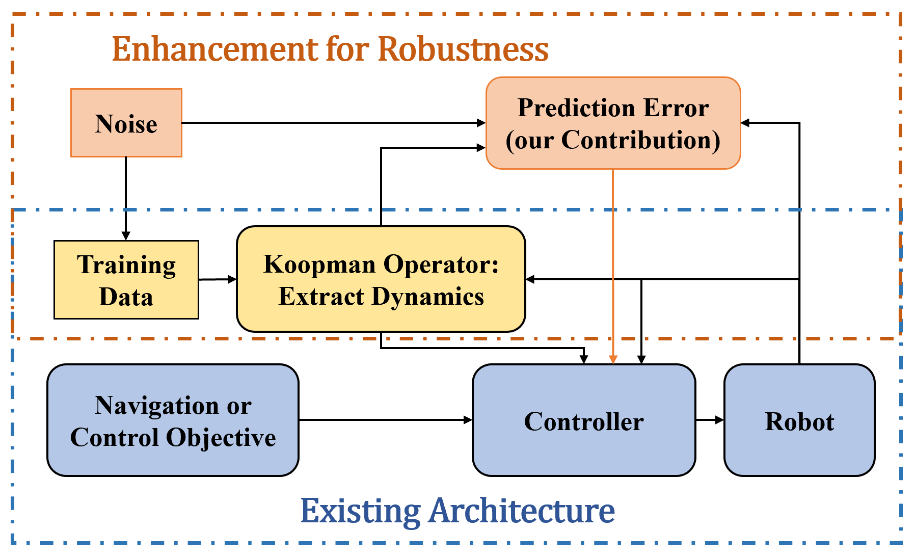
Figure 1: Overview of the enhanced robot control structure proposed in this work.

Consider the forced nonlinear dynamical system

$$x_{t+1}=f(x_{t},u_{t})\enspace,$$ (1)

where $x\in\mathbb{R}^{N_{x}}$ and $u\in\mathbb{R}^{N_{u}}$. Define a set of observables that are functions of both the states and inputs where $g:\mathbb{R}^{N_{x}}\times\mathbb{R}^{N_{u}}\to\mathbb{R}^{N_{x}+N_{u}}$. The propagation law of observables $g$ with the Koopman operator is $\mathcal{K}g(x_{t},u_{t})=g(f(x_{t},u_{t}),u_{t+1})$. Then, under the full-observability assumption such that $g(x_{t+1},u_{t+1})=[x_{t+1};u_{t+1}]$ and decomposing with $Q$ Koopman modes $v_{q}$, eigenvalues $\lambda_{q}$ and eigenfunctions $\varphi_{q}$, we obtain as in [36]:

$$[x_{t+1};u_{t+1}]=g(f(x_{t},u_{t}),u_{t+1})=\mathcal{K}g(x_{t},u_{t})$$

$$\to[x_{t+1};u_{t+1}]=\sum_{q=1}^{Q}v_{q}\lambda_{q}\varphi_{q}(x_{t},u_{t})\enspace.$$ (2)

The predicted state $x_{t+1}$ is obtained by taking the first $N_{x}$ elements of the vector in the right-hand part of (2).

Consider sets (termed snapshots) of $M+1$ state measurements and $M+1$ associated control inputs, that is $X=[x_{1},x_{2},\dots,x_{M},x_{M+1}]$, and $U=[u_{1},u_{2},\dots,u_{M},u_{M+1}]$. A way to estimate the Koopman operator $\mathcal{K}$ from $M+1$ state and control snapshots is via Extended Dynamic Mode Decomposition (EDMD). EDMD generates a finite dimensional approximation $K$ of $\mathcal{K}$. It does so by employing a dictionary of functions to lift state variables to a space where dynamics is approximately linear.

Given a dictionary of observables of size $Q$, $\mathcal{D}=\left\{\psi_{1},\psi_{2},\ldots,\psi_{Q}\right\}$, where each dictionary element $\psi_{q}$, $q=1,\ldots,Q$ is a differentiable function containing $x_{m}$ and $u_{m}$ terms, set the vector-valued dictionary as $\mathbf{\Psi}=[\psi_{1},\dots,\psi_{Q}]$.  Then the Koopman operator can be approximated by minimizing the total residual between snapshots, that is

$$J=\frac{1}{2}\sum_{m=1}^{M}\left(\mathbf{\Psi}\left(x_{m+1}\right)-\mathbf{\Psi}\left(x_{m}\right)K\right)^{2}\enspace,$$ (3)

Solving the least-square problem (3) with truncated singular value decomposition yields

$$K\triangleq\boldsymbol{G}^{\dagger}\boldsymbol{A}$$ (4)

where ^† denotes the pseudoinverse, and $G,A$ are given by

$$\begin{cases}\boldsymbol{G}=\frac{1}{M}\sum_{m=1}^{M}\mathbf{\Psi}_{m}^{*}\mathbf{\Psi}_{m}\enspace,\\ \boldsymbol{A}=\frac{1}{M}\sum_{m=1}^{M}\mathbf{\Psi}_{m}^{*}\mathbf{\Psi}_{m+1}\enspace,\end{cases}$$ (5)

with $T$ and ^∗ denoting transpose and conjugate transpose operations, respectively. (For clarity we use $\mathbf{\Psi}_{m}$ to abbreviate $\mathbf{\Psi}(x_{m},u_{m})=[\psi_{1}(x_{m},u_{m}),\ldots,\psi_{Q}(x_{m},u_{m})]$.)

Given $K$ computed via (4)–(5), the associated Koopman modes, eigenvalues and eigenfunctions are then computed as

$$\begin{cases}v_{q}=(w_{q}^{*}B)^{T}\enspace,\\ \lambda_{q}\xi_{q}=K\xi_{q}\enspace,\\ \varphi_{q}=\mathbf{\Psi}_{t}\xi_{q}\enspace,\end{cases}$$ (6)

where $\xi_{q}$ is the $q$-th eigenvector, $w_{q}$ is the $q$-th left eigenvector of $K$ scaled so $w_{q}^{T}\xi_{q}=1$, and $B$ is the matrix of appropriate weighting vectors so that $x=(\mathbf{\Psi}B)^{T}$. By plugging expressions (6) back to (2) we can then describe the evolution of the system using the estimated Koopman operator. Note that $\mathbf{\Psi}_{t}=[\psi_{1}(x_{t},u_{t}),\ldots,\psi_{Q}(x_{t},u_{t})]^{T}$, is the only term that needs (contains) information of current states. By using the Koopman operator and EDMD, all other terms can be computed from $M+1$ (training) measurements.

III Quantification of Prediction Error

The Koopman operator theory can thus be used to estimate the dynamics of a system directly from data (as described above). However, when training measurements are noisy, the prediction will be inaccurate. In this section, we present the main technical result of the paper which seeks to quantify the prediction error because of noisy measurements.

We first investigate the sensitivity of the approximated Koopman operator $K$ to noisy training measurements, followed by the sensitivity of the eigendecomposition to disturbed elements of $K$. Then, we combine them together to quantify the prediction error caused by noisy data when Koopman operator theory is employed.

III-A Sensitivity Analysis of Koopman Operator

Perturbations on an element $x_{m}^{i}$ (i.e. the $i^{th}$ state of measurement at snapshot $m$ with $i\in\{1,\ldots,N_{x}\}$), will cause an error $\Delta K^{i}$. This can be obtained by chain rule on (4) and (5) as

$$\Delta K^{i}=[\Delta k_{ab}^{i}]_{Q\times Q}=\sum_{m=1}^{M+1}\{(\frac{\partial G^{\dagger}}{\partial x_{m}^{i}}A+G^{\dagger}\frac{\partial A}{\partial x_{m}^{i}})\Delta x_{m}^{i}\}\enspace,$$ (7)

where 

$$\frac{\partial G^{\dagger}}{\partial x_{m}^{i}}=-G^{\dagger}\frac{\partial G}{\partial x_{m}^{i}}G^{\dagger} +G^{\dagger}(G^{\dagger})^{*}\left(\frac{\partial G^{*}}{\partial x_{m}^{i}}\right)\left(I-GG^{\dagger}\right)$$

$$+\left(I-G^{\dagger}G\right)\left(\frac{\partial G^{*}}{\partial x_{m}^{i}}\right)(G^{\dagger})^{*}G^{\dagger}$$

$$\frac{\partial A}{\partial x_{m}^{i}}=\begin{cases}\frac{1}{M}\mathbf{\Psi}_{m+1}^{*}\frac{\partial\mathbf{\Psi}_{m}}{\partial x_{m}}\mathbf{e_{i}},\enspace\text{if }m=1\\ \frac{1}{M}\mathbf{\Psi}_{m-1}^{*}\frac{\partial\mathbf{\Psi}_{m}}{\partial x_{m}}\mathbf{e_{i}},\enspace\text{if }m=M+1\\ \frac{1}{M}(\mathbf{\Psi}_{m+1}^{*}+\mathbf{\Psi}_{m-1}^{*})\frac{\partial\mathbf{\Psi}_{m}}{\partial x_{m}}\mathbf{e_{i}},\enspace\text{else}\end{cases}$$

and

$$\frac{\partial G}{\partial x_{m}^{i}}=\begin{cases}0,\enspace\text{if }m=M+1\\ \frac{2}{M}\mathbf{\Psi}_{m}^{*}\frac{\partial\mathbf{\Psi}_{m}}{\partial x_{m}}\mathbf{e_{i}},\enspace\text{else}\enspace.\end{cases}$$

Here $\mathbf{e_{i}}$ represents the $i^{th}$ unit vector in $\mathbb{R}^{N_{x}}$.

III-B Sensitivity Analysis of Eigendecomposition

As described in [59], if a generic element $k_{ab}$ is perturbed, the eigenvalues and eigenvectors of the matrix $K=[k_{ab}]\in\mathbb{R}^{Q\times Q}$ are affected. The sensitivity of left eigenvectors $w_{q}$, right eigenvectors $\xi_{q}$, and eigenvalues $\lambda_{q}$ can be written as

$$\begin{cases}c_{\lambda_{q}}^{ab}=\frac{\partial\lambda_{q}}{\partial k_{ab}}=w_{q}^{a}\xi_{q}^{b},\enspace(a,b,q=1,2,\dots,Q)\enspace,\\ c_{\xi_{q}}^{ab}=\frac{\partial\xi_{q}}{\partial k_{ab}}=\sum_{j=1\atop j\neq q}^{Q}h_{jq}^{ab}\xi_{j}\enspace,(a,b,q=1,2,\ldots,Q)\enspace,\\ c_{w_{q}}^{ab}=\frac{\partial w_{q}^{*}}{\partial k_{ab}}=-\sum_{j=1\atop j\neq q}^{Q}h_{qj}^{ab}w_{j}^{*}\enspace,(a,b,q=1,2,\ldots,Q)\enspace,\end{cases}$$ (8)

where $w_{q}^{a}$ denotes the $a^{th}$ element of the $q^{th}$ left-eigenvector $w_{q}$, $\xi_{q}^{b}$ is the $b^{th}$ element of the $q^{th}$ right-eigenvector $\xi_{q}$, and $h_{qj}^{ab}$ represents the $a^{th}$ row and $b^{th}$ column element of matrix $H_{qj}$ (similar for $h_{jq}^{ab}$). The matrix $H_{qj}=\left[h_{qj}^{ab}\right]_{Q\times Q}$ is computed by $\frac{w_{q}\xi_{j}^{*}}{\lambda_{j}-\lambda_{q}}$. That is, to get the eigendecomposition sensitivity of each element $k_{ab}$, we first need to obtain ($Q\times Q-Q$) $H$ matrices, and then every entry of these matrices will be used as parameters in (8).

III-C Sensitivity Analysis of Predicted Output

We are now ready to derive the perturbation in predicted outputs as a result of measurement noise. Setting $[I_{N_{x}\times N_{x}},O_{N_{x}\times N_{u}}]$ as $R$, where $I_{N_{x}\times N_{x}}$ denotes the ${N_{x}\times N_{x}}$ identity matrix and $O_{N_{x}\times N_{u}}$ denotes a ${N_{x}\times N_{x}}$ zero matrix. For the fully-observable forced nonlinear discrete time system (2), we can describe its deviation as

$$\Delta x_{t+1}=R\sum_{m=1}^{M+1}\left(\sum_{q=1}^{Q}\sum_{i=1}^{N_{x}}\frac{\partial(v_{q}\lambda_{q}\varphi_{q}(x_{t},u_{t}))}{\partial x_{m}^{i}}\Delta x_{m}^{i}\right)$$ (9)

$$=R\sum_{m=1}^{M+1}\left(\sum_{a=1}^{Q}\sum_{b=1}^{Q}\sum_{q=1}^{Q}\sum_{i=1}^{N_{x}}\frac{\partial(v_{q}\lambda_{q}\varphi_{q}(x_{t},u_{t}))}{\partial k_{ab}^{i}}\frac{\partial k_{ab}^{i}}{\partial x_{m}^{i}}\Delta x_{m}^{i}\right)$$

$$\medsize=R\sum_{a}^{Q}\sum_{b}^{Q}\left((\sum_{q}^{Q}\sum_{i}^{N_{x}}\frac{\partial(v_{q}\lambda_{q}\varphi_{q}(x_{t},u_{t}))}{\partial k_{ab}^{i}})(\sum_{m}^{M+1}\frac{\partial k_{ab}^{i}}{\partial x_{m}^{i}}\Delta x_{m}^{i})\right).$$

Letting

$$\Delta k_{ab}^{i}=\sum_{m=1}^{M+1}\frac{\partial k_{ab}^{i}}{\partial x_{m}^{i}}\Delta x_{m}^{i},$$

we deduce

$$\Delta x_{t+1}=R\sum_{a=1}^{Q}\sum_{b=1}^{Q}\left(\sum_{q=1}^{Q}\sum_{i=1}^{N_{x}}\frac{\partial(v_{q}\lambda_{q}\varphi_{q}(x_{t},u_{t}))}{\partial k_{ab}}\Delta k_{ab}^{i}\right)\enspace.$$ (10)

Note that as illustrated in (8), for a dynamical system evolving by $K$, $\frac{\partial\lambda_{q}}{\partial k_{ab}}=c_{\lambda_{q}}^{ab}$, $\frac{\partial\xi_{q}}{\partial k_{ab}}=c_{\xi_{q}}^{ab}$, and $\frac{\partial w_{q}^{T}}{\partial k_{ab}}=c_{w_{q}}^{ab}$ are finite (bounded) constants. Then, for every $k_{ab}$ we have

$$\medsize\begin{aligned} \frac{\partial(\boldsymbol{v}_{q}\lambda_{q}\varphi_{q}(x_{t},u_{t}))}{\partial k_{ab}}=\frac{\partial(\boldsymbol{v}_{q})\lambda_{q}\varphi_{q}}{\partial k_{ab}}+\frac{\boldsymbol{v}_{q}\partial(\lambda_{q})\varphi_{q}}{\partial k_{ab}}+\frac{\boldsymbol{v}_{q}\lambda_{q}\partial(\varphi_{q})}{\partial k_{ab}}\\ =((c_{w_{q}}^{ab})^{*}B)^{T}\lambda_{j}\mathbf{\Psi}_{t}\xi_{q}+(w_{q}^{*}B)^{T}c_{\lambda_{q}}^{ab}\mathbf{\Psi}_{t}\xi_{q}+(w_{q}^{*}B)^{T}\lambda_{q}\mathbf{\Psi}_{t}c_{\xi_{q}}^{ab}.\end{aligned}$$ (11)

Using matrix format of (11) and $\Delta K^{i}=[\Delta k_{ab}^{i}]_{Q\times Q}$ from (7), we can first compute the dot product of these two matrices and then obtain the prediction error as the sum of each element of the dot product, that is

$$\medsize\begin{aligned} \Delta x_{t+1}&=Re^{T}\{\left[\sum_{q=1}^{Q}\frac{\partial(\boldsymbol{v}_{q}\lambda_{q}\varphi_{q}(x_{t},u_{t}))}{\partial k_{ab}}\right]_{Q\times Q}\cdot(\sum_{i=1}^{N_{x}}\Delta K^{i})\}e\enspace,\\ \end{aligned}$$ (12)

where $e=[1,1,\dots,1]^{T}$.

It is worth noting that in our proposed formulation, $\Delta K^{i}$ is estimated using only measurements and information about the noise, so it can be obtained offline. Similarly, the eigendecomposition sensitivity analysis of $K$ is predetermined and can yield the complex parameters $c_{w_{q}}^{ab}$, $c_{\lambda_{q}}^{ab}$, $c_{\xi_{q}}^{ab}$ ahead of time. These allow part of our approach to be executed during training, and enable the computation of the prediction error to take place at run-time, to adjust to measurements errors and thus endow robustness to the overall data-driven robot control architecture (Fig. 1). Finally the perturbed prediction is written as a function of the training measurements on states and inputs ($X$, $U$) of length $M+1$ and current observation $\mathbf{\Psi}(\mathbf{x_{t}},\mathbf{u_{t}})$. For clarity of presentation, we will use the following abbreviation in the remainder of the paper

$$\Delta\mathbf{x_{t+1}}=\eta(X,U,\mathbf{\Psi}(\mathbf{x_{t}},\mathbf{u_{t}}))\enspace.$$ (13)

The relation between the offline (at training-time) and online (at run-time) components of our approach is shown in Fig. 2 and is discussed next.

IV Algorithmic Implementation

The proposed quantification of prediction error approach describes analytically how to accommodate for measurement noise in data-driven control systems that are based on the Koopman operator. To make the approach amenable to robot control applications, where real-time implementation is required, we demonstrate in this section how the most computationally-intense aspects of the proposed approach can in fact be precomputed. Then, we present the algorithmic implementation of our approach in Algorithm 1.

IV-A Enabling Real-time Operation

Reformulation of dynamics-extraction expression: Recall that only the observation at current time $t$, $\mathbf{\Psi}_{t}$, requires information gathered during run-time for making a prediction. We can thus rewrite (2) to extract the terms that can be precomputed. Consider the dynamics

$$x_{t+1}=[I_{N_{x}\times N_{x}},O_{N_{x}\times N_{u}}]\sum_{q=1}^{Q}v_{q}\lambda_{q}\varphi_{q}(x_{t},u_{t})\enspace.$$

Combining (6) yields

$$\sum_{q=1}^{Q}v_{q}\lambda_{q}\varphi_{q}(x_{t},u_{t}) =\sum_{q=1}^{P}(w_{q}^{*}B)^{T}\lambda_{q}\mathbf{\Psi}_{t}\xi_{q}$$

$$=\left(\sum_{q=1}^{Q}\left(\mathbf{\Psi}_{t}\xi_{q}\right)^{T}\left((w_{q}^{*}B)^{T}\lambda_{q}\right)^{T}\right)^{T}$$

$$=\left(\sum_{q=1}^{Q}\mathbf{\Psi}_{t}\xi_{q}\ \left((w_{q}^{*}B)^{T}\lambda_{q}\right)^{T}\right)^{T}$$

$$\to x_{t+1}=[I_{N_{x}\times N_{x}},O_{N_{x}\times N_{u}}]\left(\mathbf{\Psi}_{t}F\right)^{T}\enspace,$$ (14)

where $F=\sum_{q=1}^{Q}\xi_{q}\lambda_{q}w_{q}^{*}B$. Thus, we have separated (2) into offline ($F$) and online ($\mathbf{\Psi}_{t}$) parts.

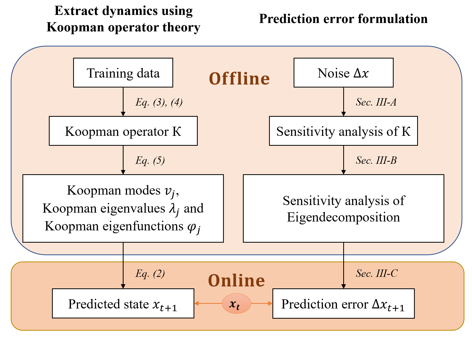
Figure 2: Illustration of the proposed approach’s pipeline to adding robustness to data-driven robot control design (c.f. top system sub-block in Fig. 1). Our approach can be decomposed into an offline and an online component for real-time implementation, specific details of which are given in Algorithm 1.

Information of noise: In the original formulation (9), we require the noise in measurements $\Delta x_{m}$ at every time instant. However, in practice we only have access to (or make assumptions about) noise statistics, for example mean $E(\Delta x)$ and standard deviation $\delta(\Delta x)$ in the case of Gaussian noise. We can thus replace each $\Delta x_{m}$ by $E(\Delta x)$ directly. Also, we can randomly sample a training dataset $\Delta X\sim(E(\Delta x),\delta^{2}(\Delta x))$, applying it to (9), and repeat the process for several times to get the average values for accuracy.

Algorithm 1 Estimation Procedure

Initialization: Collect measurements of states $X$ and
inputs $U$ that might be noisy.
Offline training:
Extracting dynamics:

• Utilize $X$, $U$ to estimate the Koopman operator $K$
  as well as matrices $G$, $A$ with (4) and (5).

• Compute parameter matrix $F$ in (14) with estimated $K$.

Estimation of prediction error:

• Obtain $\Delta K^{i}$ with information of noise in measurements and the approximated $K$, $G$, $A$ using (7).

• Get the parameters for eigendecomposition sensitivity $c_{\lambda_{q}}^{ab}$, $c_{\xi_{q}}^{ab}$ and $c_{w_{q}}^{ab}$ through (8) with estimated $K$.

Online propagation for $t$ do

       repeat

             Robotic System: Use learned prediction error $\Delta x_{t}$ at last timestep to complement model constraints used in controller design. Then, drive the robot with this control signal. Extracting dynamics:

• Use $F$ to estimate the system dynamics and
  do prediction as described in (14).

Estimate prediction error:

• Get eigen-sensitivity matrix (11) with
  pretrained
  $c_{\lambda_{q}}^{ab}$, $c_{\xi_{q}}^{ab}$, $c_{w_{q}}^{ab}$ and current observation $\mathbf{\Psi}_{t}$.

• Compute prediction error $\Delta x_{t+1}$ with $\Delta K$
  and the eigen-sensitivity matrix by (12).

$t\leftarrow t+1$

      until control task is finished;

      

V Parametric Testing and Evaluation

V-A Simulation with a Van der Pol Oscillator

To evaluate the proposed approach outlined in Algorithm 1, we first test it using the Van del Pol oscillator [47],

$$\begin{cases}\begin{array}[]{l}{\dot{x}_{1}=2x_{2}}\\ {\dot{x}_{2}=-0.8x_{1}+2x_{2}-10x_{1}^{2}x_{2}+u}\enspace.\end{array}\end{cases}$$ (15)

The system (15) is discretized with period $T_{s}=0.01$ s. $M+1$ pairs of data generated from the system are used to estimate Koopman operator $K$, and are further implemented as dynamic constraint in the controller. A random input vector is applied to propagate the system.

The whole process is implemented in a parametric study as follows. We consider four distinct cases for measurement sets with $M=\{2*10^{3},1*10^{4},2*10^{4},2*10^{5}\}$. We also consider three distinct noise levels for the disturbance. The amplitudes of the disturbances are chosen randomly from uniform distributions over the intervals $c_{1}=[0,0.1x(0)]$, $c_{2}=[0,0.2x(0)]$ and $c_{3}=[0,0.4x(0)]$ for ‘low ($10\%$),’ ‘middle ($20\%$)’ and ‘high ($40\%$)’ noise levels, respectively. These to lead to a total of $12$ distinct case studies. For each case study, we train the system according to the selected measurements and noise settings, then give a random input vector to propagate the trained system for $50$ time steps, collect the output, and finally measure the true and predicted errors. To avoid bias and randomness, we evaluate the trained system under each case study in $5$ repeated trials, and averaged results are reported. For instance, Fig. 3 shows the average predicted error and the average true error when $M=2*10^{4}$ and under the $c_{2}$ noise case (middle).

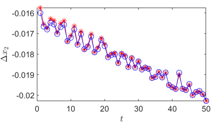
Figure 3: Prediction (blue circle) and true (red star) error under middle level noise ($c_{2}$) when $M=2*10^{4}$.

To compare overall the cases, we define the Mean Squared Error (MSE) between the estimated and true prediction error as

$$MSE=\frac{1}{50}\sum_{t=1}^{50}(\Delta x_{2}^{\mathrm{prediction}}(t)-(\Delta x_{2}^{\mathrm{true}}(t))^{2}\enspace.$$ (16)

Results (averaged $MSE$) are depicted and compared in Fig 4. We observe that 1) low density noise leads to smaller prediction error for most choices of $M$. 2) Our method performs better with a large enough size of training data set (e.g., greater than $2*10^{4}$ as shown in the simulation). 3) If we keep increasing the size (e.g., $5*10^{4}$ in this one), its accuracy may not be improved further.

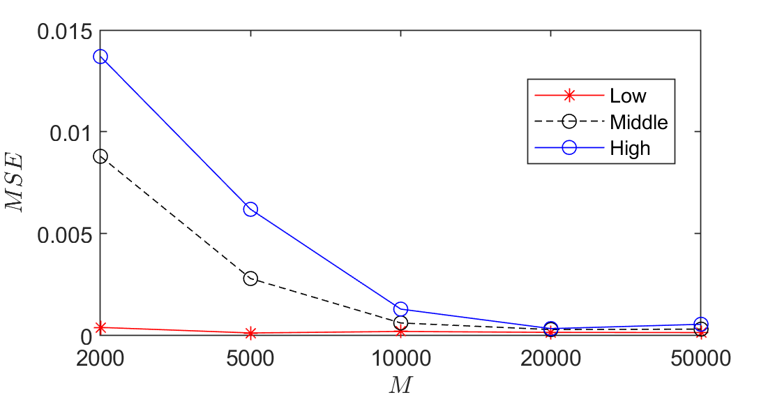
Figure 4: Mean Squared Error (MSE) of estimated and true prediction error under different noise levels.

V-B Simulation Experiments with a Wheeled Robot

Simulation experiments are conducted in the Gazebo environment using a ROSbot 2.0 robot, a differential-drive wheeled robot (Fig. 5). The ROSbot 2.0 is an autonomous, open source robot platform and the embedded software allow us to send motion commands by manipulating the $x$ component of linear speed vector as $u_{x}$ and the $z$ component of the angular speed vector as $u_{z}$. The state vector contains the geometric center position $\{x,y\}$ and orientation $\theta$.

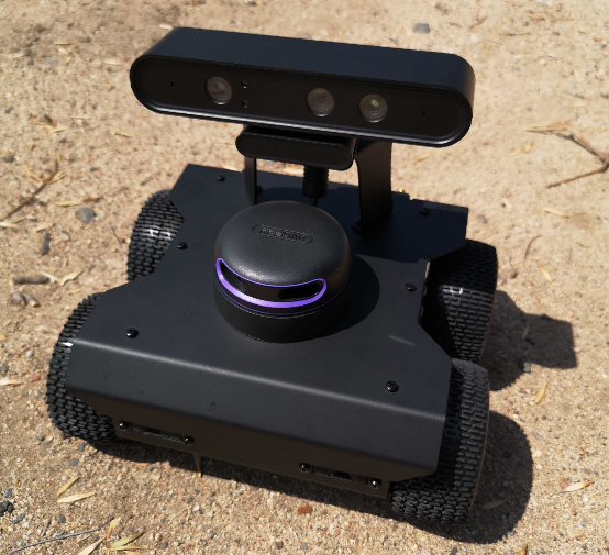
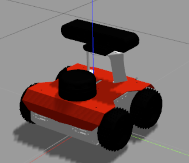
Figure 5: ROSbot 2.0 and its Gazebo model.

We test the efficiency of our proposed approach by building on top of an existing Koopman operator based controller [11], which is a data-driven hierarchical structure that refines the nominal input $u_{o}$ as $\hat{u}=u(K,u_{o})$ to improve the performance of the controller under uncertainty. We highlight that the relation between inputs $u$ and the states $x$ is learned using the Koopman operator, and then the learned model is used to get a predicted (refined) input signal $\hat{u}$. Accurate and noisy data are used to generate the deterministic Koopman operator $K$ and stochastic one $K_{n}$. Then, these two are worked as model constraints to design the ‘Nominal’ and ‘Noisy’ controllers separately. To reduce the effect of noise in the learned model $K_{n}$, which is the contribution of our paper, we try to learn the prediction error generated by $K_{n}$ using Algorithm 1. Then, this prediction error is used to complement the ‘Noisy’ controller to yield the ‘Proposed’ control signal.

We compute the approximated Koopman operator using data captured when the robot is operating in open loop based on a random chattering linear velocity and angular velocity input signals. We perform $10$ such open-loop trials. The noisy training data set is created by adding disturbance in the position states $x$ and $y$. We sample the magnitude of noise for each state from the uniform distribution over the interval $c_{1}=[0,0.25\max(\xi_{r})]$, $c_{2}=[0,0.50\max(\xi_{r})]$, $c_{3}=[0,0.75\max(\xi_{r})]$, $c_{4}=[0,1.00\max(\xi_{r})]$.

During testing, the robot is required to follow a semicircle trajectory for length $\frac{T}{2}$, i.e. $[x_{r},y_{r}]=[\sin(\frac{2\pi}{T}t),1-cos(\frac{2\pi}{T}t)]$. To avoid bias, testing trials are repeated for $10$ consecutive times for an average with the same training set. We compute the Mean Squared Error (MSE) for the direct prediction error of $u_{x}$ and $u_{z}$ as defined in (16), where the prediction term is $\Delta u$ and the true term is $(u(K_{n})-u(K)$ and the results are illustrated in Fig. 6. We also obtain the difference among all trials for the output trajectories and show the results of position $x$ as well as $y$ in Fig. 7. It can be observed that, 1) our proposed method can approximate the prediction uncertainty because of noise with a small error (Fig. 6). 2) When we implement the estimated uncertainty to a Koopman-based data-driven structure, our ‘Proposed’ controller can drive the ‘Noisy’ one closer to a desired trajectory. 3) As the noise level increases, our approach performs worse in terms of the prediction error estimation while performs better when we use the estimation for control. 4) Our algorithm remains bounded to the performance of the nominal controller (as the ‘$25\%$‘ noise level case in Fig. 7). Ongoing work focuses on implementation in different types of Koopman operator-based nominal controllers.

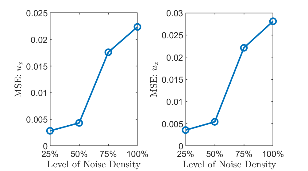
Figure 6: Mean Squared Error (MSE) of the estimated and true prediction error for linear velocity (left panel) and angular velocity (right panel) under different levels of noise.

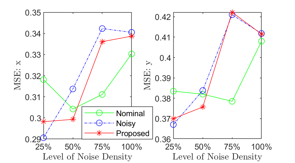
Figure 7: MSE of output trajectories’ evolution along the $x$ axis (left panel) and $y$ axis (right panel) under distinct noise levels.

VI Conclusions

In this paper we focus on motion control of data-driven systems that are based on the Koopman operator theory to extract system models from data. We investigate the prediction error of a perturbed systems’ performance when the data used for training the Koopman operator are noisy. The prediction error is then used to develop a new enhanced mobile robot motion control algorithm that endows robustness to data-driven systems. We show how certain aspects of our approach can happen offline, thus making the proposed algorithm amenable to real-time implementation. We test the proposed approach in a parametric simulated study using a Van der Pol oscillator to evaluate its performance as the number of training data and the level of noise corrupting them vary. We further test in Gazebo simulation with a non-holonomic wheeled robot tasked to track a reference trajectory. Results from both types of testing confirm that the proposed approach can apply across systems, including practical robotics.

In all, our work provides robustness guarantees for systems using Koopman operator for control, and it can be viewed as a step toward developing new motion planners and controllers for data-driven mobile robots. Future research directions include integration with motion planning algorithms, and porting from Gazebo to hardware implementation.

References

- [1] S. M. LaValle, Planning Algorithms. Cambridge, U.K.: Cambridge University Press, 2006, available at http://planning.cs.uiuc.edu/.
- [2] S. Sharma, “Autonomous waypoint generation with safety guarantees: On-line motion planning in unknown environments,” arXiv preprint arXiv:1709.00546, 2017.
- [3] L. Zheng, J. Pan, R. Yang, H. Cheng, and H. Hu, “Learning-based safety-stability-driven control for safety-critical systems under model uncertainties,” arXiv preprint arXiv:2008.03421, 2020.
- [4] R. R. Da Silva, S. Silva, G. Dubrovskiy, and H. Lin, “Safeguardpf: Safety guaranteed reactive potential fields for mobile robots in unknown and dynamic environments,” arXiv preprint arXiv:1609.07006, 2016.
- [5] G. Aoude, B. Luders, J. M. Joseph, N. Roy, and J. P. How, “Probabilistically Safe Motion Planning to Avoid Dynamic Obstacles with Uncertain Motion Patterns.” Autonomous Robots, vol. 35, pp. 51–76, 2013.
- [6] A. Shkolnik, M. Levashov, I. R. Manchester, and R. Tedrake, “Bounding on rough terrain with the LittleDog robot,” The International Journal of Robotics Research, vol. 30, no. 2, pp. 192–215, 2011.
- [7] F. Qian, T. Zhang, C. Li, P. Masarati, A. Hoover, P. Birkmeyer, A. Pullin, R. Fearing, and D. Goldman, “Walking and runnign on yielding and fluidizing ground,” in Proceedings of Robotics: Science and Systems, 2012, pp. 345–352.
- [8] S. Zarovy, M. Costello, A. Mehta, G. Gremillion, D. Miller, B. Ranganathan, J. S. Humbert, and P. Samuel, “Experimental study of gust effects on micro air vehicles,” in AIAA Conference on Atmospheric Flight Mechanics., 2010, pp. AIAA–2010–7818.
- [9] C. Powers, D. Mellinger, A. Kushleyev, B. Kothmann, and V. Kumar, “Influence of aerodynamics and proximity effects in quadrotor flight,” in Proceedings of the International Symposium on Experimental Robotics, ser. Springer Tracts in Advanced Robotics, vol. 88, 2012, pp. 289–302.
- [10] X. Kan, H. Teng, and K. Karydis, “Online exploration and coverage planning in unknown obstacle-cluttered environments,” IEEE Robotics and Automation Letters, vol. 5, no. 4, pp. 5969–5976, 2020.
- [11] L. Shi, H. Teng, X. Kan, and K. Karydis, “A data-driven hierarchical control structure for systems with uncertainty,” in 2020 IEEE Conference on Control Technology and Applications (CCTA). IEEE, 2020, pp. 57–63.
- [12] A. A. Pereira, J. Binney, G. A. Hollinger, and G. S. Sukhatme, “Risk-aware Path Planning for Autonomous Underwater Vehicles using Predictive Ocean Models,” Journal of Field Robotics, vol. 30, no. 5, pp. 741–762, 2013.
- [13] R. Alterovitz, M. Branicky, and K. Goldberg, “Motion Planning Under Uncertainty for Image-guided Medical Needle Steering,” The International Journal of Robotics Research, vol. 27, no. 11-12, pp. 1361–1374, 2008.
- [14] A. Timcenko and P. Allen, “Modeling dynamic uncertainty in robot motions,” in Proceedings of the IEEE International Conference on Robotics and Automation, 1993, pp. 531–536.
- [15] S. Thrun, W. Burgard, and D. Fox, Probabilistic Robotics (Intelligent Robotics and Autonomous Agents). The MIT Press, 2005.
- [16] G. S. Chirikjian, Stochastic Models, Information Theory, and Lie Groups, Volume 2: Analytic Methods and Modern Applications. Birkhauser, 2012.
- [17] K. Karydis, I. Poulakakis, J. Sun, and H. G. Tanner, “Probabilistically valid stochastic extensions of deterministic models for systems with uncertainty,” The International Journal of Robotics Research, vol. 34, no. 10, pp. 1278–1295, 2015.
- [18] H. Abdulsamad and J. Peters, “Hierarchical decomposition of nonlinear dynamics and control for system identification and policy distillation,” arXiv preprint arXiv:2005.01432, 2020.
- [19] V. Sindhwani, H. Sidahmed, K. Choromanski, and B. Jones, “Unsupervised anomaly detection for self-flying delivery drones,” in IEEE International Conference on Robotics and Automation (ICRA). IEEE, 2020, pp. 186–192.
- [20] J. Schmidhuber, “Deep learning in neural networks: An overview,” Neural networks, vol. 61, pp. 85–117, 2015.
- [21] E. Kaiser, J. N. Kutz, and S. L. Brunton, “Data-driven approximations of dynamical systems operators for control,” arXiv preprint arXiv:1902.10239, 2019.
- [22] H. Suprijono and B. Kusumoputro, “Direct inverse control based on neural network for unmanned small helicopter attitude and altitude control,” Journal of Telecommunication, Electronic and Computer Engineering (JTEC), vol. 9, no. 2-2, pp. 99–102, 2017.
- [23] G. Shi, X. Shi, M. O’Connell, R. Yu, K. Azizzadenesheli, A. Anandkumar, Y. Yue, and S.-J. Chung, “Neural lander: Stable drone landing control using learned dynamics,” in IEEE International Conference on Robotics and Automation (ICRA), 2019, pp. 9784–9790.
- [24] G. Shi, W. Hönig, Y. Yue, and S.-J. Chung, “Neural-swarm: Decentralized close-proximity multirotor control using learned interactions,” arXiv preprint arXiv:2003.02992, 2020.
- [25] A. J. Taylor, V. D. Dorobantu, H. M. Le, Y. Yue, and A. D. Ames, “Episodic learning with control lyapunov functions for uncertain robotic systems,” arXiv preprint arXiv:1903.01577, 2019.
- [26] H. Cui, T. Nguyen, F.-C. Chou, T.-H. Lin, J. Schneider, D. Bradley, and N. Djuric, “Deep kinematic models for kinematically feasible vehicle trajectory predictions,” in 2020 IEEE International Conference on Robotics and Automation (ICRA). IEEE, 2020, pp. 10 563–10 569.
- [27] P. L. Bartlett, D. J. Foster, and M. J. Telgarsky, “Spectrally-normalized margin bounds for neural networks,” in Advances in Neural Information Processing Systems, 2017, pp. 6240–6249.
- [28] A. Aswani, H. Gonzalez, S. S. Sastry, and C. Tomlin, “Provably safe and robust learning-based model predictive control,” Automatica, vol. 49, no. 5, pp. 1216–1226, 2013.
- [29] F. Berkenkamp, M. Turchetta, A. Schoellig, and A. Krause, “Safe model-based reinforcement learning with stability guarantees,” in Advances in neural information processing systems, 2017, pp. 908–918.
- [30] J. F. Fisac, A. K. Akametalu, M. N. Zeilinger, S. Kaynama, J. Gillula, and C. J. Tomlin, “A general safety framework for learning-based control in uncertain robotic systems,” IEEE Transactions on Automatic Control, vol. 64, no. 7, pp. 2737–2752, 2018.
- [31] F. Berkenkamp and A. P. Schoellig, “Safe and robust learning control with gaussian processes,” in European Control Conference (ECC). IEEE, 2015, pp. 2496–2501.
- [32] A. K. Akametalu, J. F. Fisac, J. H. Gillula, S. Kaynama, M. N. Zeilinger, and C. J. Tomlin, “Reachability-based safe learning with gaussian processes,” in 53rd IEEE Conference on Decision and Control, 2014, pp. 1424–1431.
- [33] A. Chatterjee, “An introduction to the proper orthogonal decomposition,” Current science, pp. 808–817, 2000.
- [34] K. Karydis and M. A. Hsieh, “Uncertainty quantification for small robots using principal orthogonal decomposition,” in International Symposium on Experimental Robotics. Springer, 2016, pp. 33–42.
- [35] J. H. Tu, C. W. Rowley, D. M. Luchtenburg, S. L. Brunton, and J. N. Kutz, “On dynamic mode decomposition: theory and applications,” arXiv preprint arXiv:1312.0041, 2013.
- [36] M. O. Williams, I. G. Kevrekidis, and C. W. Rowley, “A data–driven approximation of the koopman operator: Extending dynamic mode decomposition,” Journal of Nonlinear Science, vol. 25, no. 6, pp. 1307–1346, 2015.
- [37] S. Klus, F. Nüske, S. Peitz, J.-H. Niemann, C. Clementi, and C. Schütte, “Data-driven approximation of the koopman generator: Model reduction, system identification, and control,” Physica D: Nonlinear Phenomena, vol. 406, p. 132416, 2020.
- [38] E. Kaiser, J. N. Kutz, and S. L. Brunton, “Data-driven discovery of koopman eigenfunctions for control,” arXiv preprint arXiv:1707.01146, 2017.
- [39] C. Folkestad, D. Pastor, I. Mezic, R. Mohr, M. Fonoberova, and J. Burdick, “Extended dynamic mode decomposition with learned koopman eigenfunctions for prediction and control,” arXiv preprint arXiv:1911.08751, 2019.
- [40] S. L. Brunton, B. W. Brunton, J. L. Proctor, and J. N. Kutz, “Koopman invariant subspaces and finite linear representations of nonlinear dynamical systems for control,” PloS one, vol. 11, no. 2, 2016.
- [41] B. O. Koopman, “Hamiltonian systems and transformation in hilbert space,” Proceedings of the National Academy of Sciences of the United States of America, vol. 17, no. 5, p. 315, 1931.
- [42] B. Huang, X. Ma, and U. Vaidya, “Data-driven nonlinear stabilization using koopman operator,” arXiv preprint arXiv:1901.07678, 2019.
- [43] I. Abraham and T. D. Murphey, “Active learning of dynamics for data-driven control using koopman operators,” IEEE Transactions on Robotics, vol. 35, no. 5, pp. 1071–1083, 2019.
- [44] I. Abraham, G. De La Torre, and T. D. Murphey, “Model-based control using koopman operators,” arXiv preprint arXiv:1709.01568, 2017.
- [45] D. Bruder, B. Gillespie, C. D. Remy, and R. Vasudevan, “Modeling and control of soft robots using the koopman operator and model predictive control,” arXiv preprint arXiv:1902.02827, 2019.
- [46] H. Arbabi, M. Korda, and I. Mezic, “A data-driven koopman model predictive control framework for nonlinear flows,” arXiv preprint arXiv:1804.05291, 2018.
- [47] M. Korda and I. Mezić, “Linear predictors for nonlinear dynamical systems: Koopman operator meets model predictive control,” Automatica, vol. 93, pp. 149–160, 2018.
- [48] G. Mamakoukas, M. L. Castano, X. Tan, and T. D. Murphey, “Derivative-based koopman operators for real-time control of robotic systems,” arXiv preprint arXiv:2010.05778, 2020.
- [49] D. Bruder, C. D. Remy, and R. Vasudevan, “Nonlinear system identification of soft robot dynamics using koopman operator theory,” in IEEE International Conference on Robotics and Automation (ICRA), 2019, pp. 6244–6250.
- [50] M. L. Castaño, A. Hess, G. Mamakoukas, T. Gao, T. Murphey, and X. Tan, “Control-oriented modeling of soft robotic swimmer with koopman operators,” in IEEE/ASME International Conference on Advanced Intelligent Mechatronics (AIM), 2020, pp. 1679–1685.
- [51] A. Broad, I. Abraham, T. Murphey, and B. Argall, “Data-driven koopman operators for model-based shared control of human–machine systems,” The International Journal of Robotics Research, p. 0278364920921935, 2020.
- [52] M. Korda and I. Mezić, “On convergence of extended dynamic mode decomposition to the koopman operator,” Journal of Nonlinear Science, vol. 28, no. 2, pp. 687–710, 2018.
- [53] S. Peitz and S. Klus, “Koopman operator-based model reduction for switched-system control of pdes,” Automatica, vol. 106, pp. 184–191, 2019.
- [54] G. Mamakoukas, I. Abraham, and T. D. Murphey, “Learning stable models for prediction and control,” 2020.
- [55] K. Zhou and J. C. Doyle, Essentials of robust control. Prentice hall Upper Saddle River, NJ, 1998, vol. 104.
- [56] J. L. Proctor, S. L. Brunton, and J. N. Kutz, “Generalizing koopman theory to allow for inputs and control,” SIAM Journal on Applied Dynamical Systems, vol. 17, no. 1, pp. 909–930, 2018.
- [57] M. O. Williams, M. S. Hemati, S. T. Dawson, I. G. Kevrekidis, and C. W. Rowley, “Extending data-driven koopman analysis to actuated systems,” IFAC-PapersOnLine, vol. 49, no. 18, pp. 704–709, 2016.
- [58] G. H. Golub and V. Pereyra, “The differentiation of pseudo-inverses and nonlinear least squares problems whose variables separate,” SIAM Journal on numerical analysis, vol. 10, no. 2, pp. 413–432, 1973.
- [59] T. Crossley and B. Porter, “Eigenvalue and eigenvector sensitivities in linear systems theory,” International Journal of Control, vol. 10, no. 2, pp. 163–170, 1969.