Quantum potentiality in Inhomogeneous Cosmology

Abstract

For the Szekeres system which describes inhomogeneous and anisotropic spacetimes we make use of a point-like Lagrangian, which describes the evolution of the physical variables of the Szekeres model, in order to perform a canonical quantization and to study the quantum potentiality of the Szekeres system in the content of de Broglie–Bohm theory. We revise previous results on the subject and we find that for a specific family of trajectories with initial conditions which satisfy a constraint equation, there exists additional conservation laws for the classical Szekeres system which are used to define differential operators and to solve the Wheeler-DeWitt equation. From the new conservation laws we construct a wave function which provides a nonzero quantum potential term that modifies the Szekeres system. The quantum potential corresponds to new terms in the dynamical system such that new asymptotic solutions with a nonzero energy momentum tensor of an anisotropic fluid exist. Therefore, the silent property of the Szekeres spacetimes is violated by quantum correction terms.

I Introduction

Quantum gravity is motivated by the idea to have a quantum description of all the matter fields and of their interactions in a gravitational system rqc1 . The dynamical variables of the spacetime interact with the matter fields as is described by General Relativity. Hence, in quantum gravity the dynamical variables of the spacetimes are described by quantum physics. The study of the quantum properties of the whole universe as a unique gravitational system is part of quantum cosmology. For extended discussions we refer the reader to rqc1 ; rqc2 . In this work we are interested in the analytic solutions of the Wheeler-DeWitt equation wdw1 ; wdw2 for quantum cosmology in the case of inhomogeneous spacetimes and in the derivation of quantum corrections on the semiclassical limit as described by de Broglie–Bohm theory bm1 ; bm2 ; bm3 ; bm4 ; bm5 .

Inhomogeneous cosmological models are exact spacetimes which in general do not admit any isometry vector field while the conditions described by the cosmological principle, that is, the limit of the Friedmann–Lemaître–Robertson–Walker universe is provided kras . Inhomogeneous cosmological models can be used for the description of the universe in the preinflationary era dd1 ; dd2 ; dd3 ; dd4 ; dd5 , as also in the description of the small inhomogeneities which are found by cosmological observations dd6 ; dd7 ; dd8 ; dd9 ; dd10 . This is an alternative approach based on exact solutions and is different from the cosmological perturbation theory.

In the following we are interested in Szekeres spacetimes szek . These spacetimes are exact solutions of the gravitational field equations for a diagonal line element with two dynamical variables and zero magnetic component for the Weyl tensor. The matter field is described by an inhomogeneous pressureless fluid. Szekeres spacetimes are characterized as “partially locally rotational” spacetimes silent0 . The term “partially” indicates that the exact solutions do not admit any isometry vector field. Furthermore, there is no information dissemination with gravitational or sound waves on these exact solutions which means that they are silent universes silent . There are various interesting results in the literature which have shown that Szekeres spacetimes can play a significant role in the description of various epochs of our universe per101 ; per102 ; per103 ; per104 , while the present isotropic and homogeneous on large scales observed universe can be provided by Szekeres spacetimes for specific initial conditions with or without an inflationary era in the cosmological evolution bbb01 ; bbb02 ; bbb03 . Various generalizations of the Szekeres spacetimes with other kind of matter fields can be found in sz1 ; sz2 ; sz3 ; sz4 ; sz9 ; sz10 ; sz11 .

Szekeres universes are described by (pseudo)-Riemannian geometry with line element $ds^{2}=g_{\mu\nu}dx^{\mu}dx^{\nu}$, $x^{\mu}=\left(t,x,y,z\right)$ and

$$g_{\mu\nu}=diag\left(-1,e^{2\alpha\left(t,x,y,z\right)},e^{2\beta\left(t,x,y,z\right)},e^{2\beta\left(t,x,y,z\right)}\right),$$ (1)

where functions $\alpha\left(t,x,y,z\right)$ and $\beta\left(t,x,y,z\right)$ satisfy the following algebraic-differential system known as the Szekeres system. The first-order differential equations are

$$\dot{\rho}+\theta\rho =0,$$ (2)

$$\dot{\theta}+\frac{\theta^{2}}{3}+6\sigma^{2}+\frac{1}{2}\rho =0,~{}$$ (3)

$$\dot{\sigma}-\sigma^{2}+\frac{2}{3}\theta\sigma+E =0,$$ (4)

$$\dot{E}+3E\sigma+\theta E+\frac{1}{2}\rho\sigma =0$$ (5)

with the algebraic constraint

$$\frac{\theta^{2}}{3}-3\sigma^{2}+\frac{{}^{\left(3\right)}R}{2}=\rho,$$ (6)

where $\theta=\left(\frac{\partial\alpha}{\partial t}\right)+2\left(\frac{\partial\beta}{\partial t}\right)~{}~{}$ and $~{}\sigma^{2}=\frac{2}{3}\left(\left(\frac{\partial\alpha}{\partial t}\right)-\left(\frac{\partial\beta}{\partial t}\right)\right)^{2}$ are the expansion rate and the anisotropic parameter, $\rho=\rho\left(t,x,y,z\right)$ is the energy density of the inhomogeneous dust fluid and $E=E\left(t,x,y,z\right)$ is the electric component of the Weyl tensor $E_{\nu}^{\mu}=$ $Ee_{\nu}^{\mu};$ and ${}^{\left(3\right)}R$ is the spatial curvature of the three-dimensional hypersurface. In addition to the latter system, the dynamical variables satisfy the propagation equations which are $h_{\mu}^{\nu}\sigma_{\nu;\alpha}^{\alpha}=\frac{2}{3}h_{\mu}^{\nu}\theta_{;\nu}$ ,$~{}h_{\mu}^{\nu}E_{\nu;\alpha}^{\alpha}=\frac{1}{3}h_{\mu}^{\nu}\rho_{;\nu}$ in which $h_{\mu\nu}$ is the decomposable tensor defined by the expression $h_{\mu\nu}=g_{\mu\nu}-u_{\mu}u_{\nu}$, where $u^{\mu}$ is a unitary vector field, $u^{\mu}u_{\mu}=-1,$ which defines the physical observer lesame .

The integrability properties of the Szekeres system have been widely studied in the literature isz1 ; isz2 ; isz3 , In isz1 the Szekeres system has been written as a system of two second-order differential equations and a conservation law quadratic in the derivatives of the dynamical variables was derived. The gravitational field equations of the Szekeres model do not admit a minisuperspace description. However, as was shown in isz1 , the time-dependent field equations can be described by a point-like Lagrangian with respect to the variables $\left\{\rho,E\right\}$, while the conservation law quadratic in the derivatives is derived easily with the use of Noether’s theorem. In addition in this work we show that the Szekeres system admits as an additional conservation law the Lewis invariant.

The Lagrangian description of the Szekeres system and the Noetherian conservation law were applied in isz4 to quantize and write the “time”-independent Wheeler-DeWitt equation for the Szekeres system. The solution of the Wheeler-DeWitt equation which satisfies the quadratic conservation law has been found which does not affect the classical trajectories of the Szekeres system and there is no any quantum potential term provided. Moreover, a probability function was found from which it was found that a stationary surface of the probability function is related with classical exact solutions. A similar study was performed recently for the Szekeres system with the cosmological constant term isz5 .

In the following we revise the analysis of isz4 . Specifically, we find that, in the special case for which the “energy” of the two-dimensional Hamiltonian system which describes the Szekeres system vanishes, new conservation laws exist for the Szekeres system. These new conservation laws are used to define  quantum operators which are used as supplementary conditions on the Wheeler-DeWitt equation and to determine new similarity solutions for the Wheeler-DeWitt equation qu3 ; qu4 ; qu5 . From the new wavefunction we are able to construct a nontrivial quantum potential given by the Broglie–Bohm theory. The effects of the quantum correction in the original Szekeres system is investigated as also the effects on the dynamics are studied. The plan of the paper is as follows.

In Section II, we present the two-dimensional Hamiltonian dynamical system which is equivalent to the Szekeres system (2)-(5) and we derive the new conservation laws. In particular, we show that the Szekeres system admits as conservation law the Lewis invariant as also a family of conservation laws generated by Lie point symmetries when the energy of the Hamiltonian dynamical system is zero. The new conservation laws are applied for the derivation of quantum operators and for the derivation of exact solutions of the Wheeler-DeWitt equation in Section III. The quantum potential is determined in IV, in which we show that a nonzero quantum correction exists for specific trajectories of the Szekeres system satisfying a specific set of initial conditions. In Section V, we study the effects of the nonzero quantum correction in the Szekeres system. We write the modified Szekeres system for which a contribution in the equation for the expansion rate $\theta~{}$follows by quantum corrections. This new term modifies the dynamics of the Szekeres system and leads to new asymptotic solutions with nonzero matter, pressure and anisotropic component of an energy momentum tensor. These latter fluid components have their origin in the quantum corrections as provided by Bohmian mechanics. Finally, in Section VI, we summarize our results and we draw our conclusions.

II Hamiltonian formulation of the Szekeres system

From equations (2) and (5) we find that

$$\theta=-\frac{\dot{\rho}}{\rho}~{},~{}\sigma=\frac{2\left(\dot{\rho}E\mathcal{-}\rho\dot{E}\right)}{\rho\left(\rho+6E\right)}~{}.$$ (7)

Thus by substituting (7) into (3) and (4) we obtain an equivalent form for the Szekeres system comprising two second-order differential equations with respect to the variables $\rho$ and $E$. The resulting equations are isz1

$$\ddot{u}+\frac{1}{u^{2}} =0,$$ (8)

$$\ddot{v}-2\frac{v}{u^{3}} =0,$$ (9)

where $\left\{u,v\right\}$ are new variables defined as isz1

$$\rho\left(u,v\right)=\frac{6}{\left(u-v\right)u^{2}}~{},\ E\left(u,v\right)=\frac{v}{u^{3}\left(v-u\right)}$$ (10)

with inverse transformation

$$u\left(\rho,E\right)=\left(\frac{\rho}{6}+E\right)^{-\frac{1}{3}}~{},~{}v\left(\rho,E\right)=-\frac{6E}{\rho}\left(\frac{\rho}{6}+E\right)^{-\frac{1}{3}}.$$ (11)

The parameters $\theta$ and $\sigma$, are expressed in terms of the new variables as

$$\theta\left(u,v,\dot{u},\dot{v}\right) =\frac{\left(3u-2v\right)\dot{u}-u\dot{v}}{u\left(u-v\right)},$$ (12)

$$\sigma\left(u,v,\dot{u},\dot{v}\right) =\frac{u\dot{v}-v\dot{u}}{3u^{2}-3uv}~{}.$$ (13)

Equation (8) can be integrated by quadratures, that is, $\int\frac{du}{\sqrt{2u^{-1}+I_{0}}}=t-t_{0}$, where $I_{0}$ is a constant of integration and a conservation law for the dynamical system (8)-(9). That is, $I_{0}=\dot{u}^{2}-2u^{-1}$. Thus by writing $u=u\left(t\right)$ in (9) we obtain a linear equation of the form $\ddot{v}+\omega\left(t\right)v=0$, $\omega\left(t\right)=-2u\left(t\right)^{-3}$.  This linear second-order equation is known as the time-dependent oscillator lt1 and it is a maximally symmetric equation. Moreover, it admits as conservation law the Lewis invariant given by the expression lt2 ; lt3 ; lt4

$$\Phi=\frac{1}{2}\left(\left(y\dot{v}-\dot{y}v\right)^{2}+\left(\frac{v}{y}\right)^{2}\right),$$ (14)

where $y\left(t\right)$ is any solution of the Ermakov-Pinney differential equation lt5 , that is,

$$\ddot{y}+\omega\left(t\right)y=\frac{1}{y^{3}}.$$ (15)

Conservation law (14) is a new conservation law found for the Szekeres system and has not been derived before. It is really a point of interest that the Lewis invariant and the Ermakov-Pinney equation appears in inhomogeneous cosmology. Previously, the Ermakov-Pinney equation has appeared and in other gravitational such in scalar tensor theories and in modified theories of gravity erm1 ; erm2 .

It is easy to observe that the Szekeres equations (8), (9) can be derived by the variation of the point-like Lagrangian isz1

$$L\left(u,\dot{u},v,\dot{v}\right)=\dot{u}\dot{v}-\frac{v}{u^{2}}$$ (16)

with Hamiltonian function

$$\mathcal{H}=p_{u}p_{v}+\frac{v}{u^{2}}\equiv h\left(u,v,p_{u},p_{v}\right),~{}$$ (17)

where

$$\dot{u}=p_{v}~{},~{}\dot{v}=p_{u}~{}$$ (18)

and

$$\dot{p}_{v}=-\frac{1}{u^{2}}~{},~{}\dot{p}_{v}=2\frac{v}{u^{3}}.$$ (19)

That is a Hamiltonian description for the Szekeres system, for which we can see that (17) is a conservation law with $h\left(u,v,p_{u},p_{v}\right)=const.$, which corresponds to the “energy” of the Hamiltonian system, because equations (8), (9) are autonomous. In terms of the momentum the conservation law $I_{0}$ becomes $I_{0}=p_{v}^{2}-2u^{-1}$, which is in involution and independent of the Hamiltonian $h$. Hence, as has found before the Szekeres system is Liouville integrable isz1 . The conservation law $I_{0}$ is related with a generalized symmetry which generates a constant transformation for the dynamical system in which the Action Integral for the Szekeres system remains invariant, that is, $I_{0}$ is a Noetherian conservation law. That is not true for the Lewis invariant (14).

The application of Noether’s theorem for point and contact transformations of the Hamiltonian system (17), (18) and (19) as was found in isz1 does not provide additional conservation laws. However, the existence of conservation laws for the trajectories with initial conditions $h=0$ has been investigated before. When $h=0$, the trajectories of the Szekeres system can be seen as “null-like” trajectories which are conformally invariant, see the discussion in mtnull ; nnull ; nnull2 .

Therefore, when $h\equiv 0$, we find that the Szekeres system (8), (9) admits the additional conservation laws

$$I_{1}=u^{2}\dot{v}~{}\text{or }I_{1}=u^{2}p_{u}~{},$$ (20)

$$I_{2}=\frac{\dot{u}}{v}~{}\text{or }I_{2}=\frac{p_{v}}{v}~{},$$ (21)

and

$$I_{3}=2u\dot{v}+v\dot{u}~{}\text{or~{}}I_{3}=2up_{u}+vp_{v}.$$ (22)

These conservation laws can be derived by the application of Noether’s theorem for a conformally related Lagrangian of function (16), while they are generated by conformal transformations of the two-dimensional flat space which defines the kinetic energy for the Lagrangian function (16).

Consider now the conformal transformation $dt=u^{2}d\tau$. The conformally equivalent Lagrangian of (16) is given by

$$\bar{L}\left(u,\frac{du}{d\tau},v,\frac{d\dot{u}}{d\tau}\right)=\frac{1}{u^{2}}\left(\frac{du}{d\tau}\right)\left(\frac{dv}{d\tau}\right)-v,$$ (23)

where now the Szekeres system becomes

$$\ddot{u}-\frac{2}{u}\dot{u}^{2}+u^{2}=0~{},~{}\ddot{v}=0.$$ (24)

Under the conformal transformation the conservation law $\bar{I}_{1}$ becomes $\bar{I}_{1}=\dot{v}$. Hence, with the use of the constraint equation $\frac{1}{u^{2}}\left(\frac{du}{d\tau}\right)\left(\frac{dv}{d\tau}\right)+v=0$, the closed-form solution of the Szekeres system is expressed as

$$u\left(\tau\right)=2\left(\left(\tau-\tau_{0}\right)^{2}+u_{1}\right)^{-1}~{},~{}v\left(t\right)=\bar{I}_{1}\left(\tau-\tau_{0}\right)\text{.}$$ (25)

Hence, we can write the closed-form solution for the original variables

$$\rho\left(\tau\right)=\frac{3\left(\left(\tau-\tau_{0}\right)^{2}+u_{1}\right)^{3}}{2\left(I_{1}\left(\tau-\tau_{0}\right)\left(\left(\tau-\tau_{0}\right)^{2}+u_{1}\right)-2\right)}~{},$$ (26)

$$E\left(\tau\right)=\frac{I_{1}\left(\tau-\tau_{0}\right)\left(\left(\tau-\tau_{0}\right)^{2}+u_{1}\right)^{4}}{8\left(I_{1}\left(\tau-\tau_{0}\right)\left(\left(\tau-\tau_{0}\right)^{2}+u_{1}\right)-2\right)}~{},$$ (27)

$$\theta\left(\tau\right)=\frac{\left(\left(\tau-\tau_{0}\right)^{2}+u_{1}\right)\left(I_{1}\left(\left(\tau-\tau_{0}\right)\left(\left(\tau-\tau_{0}\right)^{2}+u_{1}\right)^{3}-4\right)-12\left(\tau-\tau_{0}\right)\right)}{8-I_{1}\left(\left(\tau-\tau_{0}\right)^{2}+u_{1}\right)^{3}}~{},$$ (28)

$$\sigma\left(\tau\right)=\frac{I_{1}\left(\left(\tau-\tau_{0}\right)^{2}+u_{1}\right)\left(8+\left(\tau-\tau_{0}\right)\left(\left(\tau-\tau_{0}\right)^{2}+u_{1}\right)\right)}{6\left(8-I_{1}\left(\left(\tau-\tau_{0}\right)^{2}+u_{1}\right)^{3}\right)}.$$ (29)

In a similar way closed-form solutions can be found for other conformal time $dt\rightarrow d\bar{\tau}$, by using the remaining vector fields. However, they are the same solutions expressed in different coordinates. Moreover, it is important to mention here that the constants of integration and the conservation laws, are constants with respect to the derivative in time, that is, they are functions of the original coordinates of the spacetime, for instance $t_{0}=t_{0}\left(x,y,z\right)$ and $t_{0}$ is an essential integration parameter that is why we have not omitted it.

We continue our analysis by performing a canonical quantization for the Hamiltonian (17) to write the Wheeler-DeWitt equation for the Szekeres system, while we use the conservation laws related with point and contact symmetries to solve the Wheeler-DeWitt equation and write the wave function.

III The Wheeler-DeWitt equation

In terms of the $3+1$ decomposition notation of General Relativity, the Wheeler-DeWitt equation follows from the Hamiltonian constraint of the field equations wdw1 . The Wheeler-DeWitt equation is not a single differential equation, but it defines a family of equations where at every point of the 3-dimensional hypersurfaces a unique equation is defined. However, in the case of the minisuperspace approximation the infinite degrees of freedom of the superspace reduce to a finite number. Hence, instead of having an equation for each point of the hypersurface, there follows a unique equation for all of the points wdw2 .

The Szekeres system (2)-(5) does not admit a minisuperspace description. However, through the dynamical variables it can be written as a two-dimensional Hamiltonian system with constraint (17). By using that property we are able to study the quantization of the Szekeres system.  Specifically we perform a canonical quantization by promoting the Poisson brackets to commutators and the variables on the phase space into operators $x^{i}\rightarrow\hat{x}^{i}=x^{i},\ p_{i}\rightarrow\hat{p}_{i}=i\frac{\partial}{\partial x^{i}}$. Thus from the Hamiltonian (17) there follows the time-independent Schrödinger equation isz4

$$\left(-\frac{\partial}{\partial u\partial v}+\frac{v}{u^{2}}-h\right)\Psi\left(u,v\right)=0.$$ (30)

At this point we can use the conservation laws to define operators which keep invariant the Wheeler-DeWitt equation (30). For arbitrary value of $h$ from $I_{0}$, there follows the quantum operator

$$\left(\frac{\partial}{\partial v^{2}}+\frac{2}{u}+I_{0}\right)\Psi\left(u,v\right)=0~{},$$ (31)

while, when $h=0$, the additional operators

$$\left(u^{2}\frac{\partial}{\partial u}+iI_{1}\right)\Psi\left(u,v\right)=0~{},$$ (32)

$$\left(\frac{1}{v}\frac{\partial}{\partial v}+iI_{2}\right)\Psi\left(u,v\right)=0~{},$$ (33)

$$\left(2u\frac{\partial}{\partial u}+v\frac{\partial}{\partial v}+iI_{3}\right)\Psi\left(u,v\right)=0$$ (34)

exist.

With the use of one of these differential operators we can construct a solution for the Wheeler-DeWitt equation (30). These solutions are called similarity solutions because the differential operators are related with Lie symmetries for the differential equation (30).

In isz4 the differential operator (31) was applied, which provides the wavefunction

$$\Psi_{A}\left(h,I_{0},u,v\right)=\frac{\sqrt{u}}{\sqrt{2+I_{0}u}}\left(\Psi_{A}^{1}\cos f\left(u,v\right)+\Psi_{A}^{2}\sin f\left(u,v\right)\right),$$ (35)

where  $f\left(u,v\right)=\left(I_{0}^{3/2}\sqrt{u}\right)^{-1}\left((hu+I_{0}v)\sqrt{2I_{0}+I_{0}^{2}u}-2h\sqrt{u}\text{{arcsin}}\mathrm{h}\left(\sqrt{\frac{I_{0}{u}}{2}}\right)\right)~{},~{}$for $I_{0}\neq 0,$ or$~{}f\left(u,v\right)=\frac{\sqrt{2}}{3}\left(hu^{2}+3v\right)u^{-\frac{1}{2}},$ for $I_{0}=0.$ Coefficients $\Psi_{A}^{1,2}$ are constants of integration. In a similar way we can construct similarity solutions by using the other differential operators. For more details on the properties of the wavefunction (35) we refer the reader in isz4 .

For $h=0$, the wave function, $\Psi\left(u,v\right),$ which satisfies the differential operator (32) is

$$\Psi_{B}\left(I_{1},u,v\right)=\Psi_{B}^{1}\exp\left(-\frac{i}{2I_{1}}\left(v^{2}+2\frac{\left(I_{1}\right)^{2}}{u}\right)\right),$$ (36)

while from (33) we find that

$$\Psi_{C}\left(I_{2},u,v\right)=\Psi_{C}^{1}\exp\left(\frac{i}{2I_{2}}\left(\frac{2}{u}+\left(I_{2}\right)^{2}v^{2}\right)\right).$$ (37)

Furthermore from (34) there follows the wave function

$$\Psi_{D}\left(\beta,u,v\right)=\left(v^{2}u\right)^{\frac{\beta}{4}}\left(\Psi_{D}^{1}J_{\frac{\beta}{2}}\left(v\sqrt{\frac{2}{u}}\right)+\Psi_{D}^{2}Y_{\frac{\beta}{2}}\left(v\sqrt{\frac{2}{u}}\right)\right)$$ (38)

in which $J_{\alpha}\left(u,v\right)$ and $Y_{\alpha}\left(u,v\right)$ are the Bessel functions of the first and of the second kinds, respectively, and $I_{3}=-i\beta$.

In the limit for which $\sqrt{\frac{2}{u}}v\rightarrow\infty\,$, the wave function (38) is approximated by the functional form

$$\hat{\Psi}_{D}\left(\beta,u,v\right)=v^{\frac{\beta-1}{2}}u^{\frac{\beta+1}{4}}\left(\hat{\Psi}_{D}^{1}\exp\left(i\left(\sqrt{\frac{2}{u}}v-\left(\beta+1\right)\frac{\pi}{4}\right)\right)+\hat{\Psi}_{D}^{2}\exp\left(-i\left(\sqrt{\frac{2}{u}}v-\left(\beta+1\right)\frac{\pi}{4}\right)\right)\right),$$ (39)

where $\hat{\Psi}_{D}^{1},~{}\hat{\Psi}_{D}^{2}$ are constants. Function $\hat{\Psi}_{D}\left(\beta,u,v\right)$ describes oscillations of the polar form $\Psi\left(u,v\right)=\Omega\left(u,v\right)e^{iS\left(u,v\right)}$ with amplitude $\Omega\left(u,v\right)=v^{\frac{\beta-1}{2}}u^{\frac{\beta+1}{4}}$ and radial argument $S\left(u,v\right)=\left(\sqrt{\frac{2}{u}}v-\left(\beta+1\right)\frac{\pi}{4}\right)$.

IV Quantum potential

In Bohmian quantum theory, the main difference from the classical theory is the quantum Hamilton-Jacobi equation which for a wave function expressed in the Madelung representaiton $\Psi\left(\mathbf{y}\right)=\Omega\left(\mathbf{y}\right)e^{iS\left(\mathbf{y}\right)}$ is defined as

$$\frac{1}{2}G^{AB}\partial_{A}S\left(\mathbf{y}\right)\partial_{B}S\left(\mathbf{y}\right)+V\left(\mathbf{y}\right)+h+Q_{V}\left(\mathbf{y}\right)=0,$$ (40)

where the term $Q_{V}\left(\mathbf{y}\right)~{}$ is known as the quantum potential and is related with the amplitude of the wave function

$$Q_{V}\left(\mathbf{y}\right)=-\frac{\Box\Omega\left(\mathbf{y}\right)}{2\Omega\left(\mathbf{y}\right)}$$ (41)

and $\Box~{}$is the Laplacian of the time-independent Schrödinger equation, that is, for our model, $\Box=\frac{\partial}{\partial u\partial v}$. The radial argument play the role of the Action, so that the canonical momentum is given as $p_{A}=\frac{\partial S}{\partial y^{A}}$. In the WKB approximation the quantum potential it is neglected and the classical limit is recovered. The Madelung representation is an alternative way to write the Schrödinger equation in a real and complex imaginary part md1 .

We continue with the calculation of the quantum potential for the wave functions which were found above.

For the wave function $\Psi_{A}\left(u,v\right)$ in isz4 it was found that there is no nonzero corresponding quantum potential. Wave functions $\Psi_{B}\left(u,v\right),~{}\Psi_{C}\left(u,v\right)$ are already written in polar form with constant amplitudes. Hence the quantum potential related with these wave functions is zero.

However, from the wave function $\Psi_{D}\left(u,v\right)$ and in the limit $\sqrt{\frac{2}{u}}v\rightarrow\infty$ which is expressed in polar form from the amplitude $\Omega\left(u,v\right)=v^{\frac{\gamma-1}{2}}u^{\frac{\gamma+1}{4}}$ the quantum potential term is

$$Q_{V}\left(u,v\right)=\frac{Q_{0}}{uv}~{}\text{with }Q_{0}=-\frac{\left(\beta^{2}-1\right)}{8}\text{. }$$ (42)

Therefore, for the trajectories with $h=0$, a quantum correction term exists. Below, we continue our analysis with the study of the effects of the quantum corrections on the original variables and how the Szekeres system is modified.

V The modified Szekeres system

With the use of the quantum potential the Hamiltonian equivalent of the Szekeres system (17) is modified to be

$$\mathcal{H}=p_{u}p_{v}+\frac{v}{u^{2}}+\frac{Q_{0}}{uv}\equiv 0.$$ (43)

Thus the equations of motion are

$$\dot{u}=p_{v}~{},~{}\dot{v}=p_{u}~{}$$ (44)

and

$$\dot{p}_{v}=-\frac{1}{u^{2}}+\frac{Q_{0}}{uv^{2}}~{},~{}\dot{p}_{v}=2\frac{v}{u^{3}}+\frac{Q_{0}}{u^{2}v}.$$ (45)

Therefore with the use of the inverse transformation from the variables $\left\{u,v,\dot{u},\dot{v}\right\}\rightarrow\left\{\rho,E,\theta,\sigma\right\}$ as is given by expressions (11), (12) and (13) we find that the only equation of the Szekeres system which is modified is equation (3) which becomes

$$\dot{\theta}+\frac{\theta^{2}}{3}+6\sigma^{2}+\frac{1}{2}\rho+\frac{Q_{0}}{72}\frac{\rho^{2}}{E^{2}}\left(\rho+6E\right)^{\frac{4}{3}}=0.$$ (46)

Because we are working in the limit where $\sqrt{\frac{2}{u}}v\rightarrow\infty$, it follows that $\sqrt{\frac{2}{u}}v=-\frac{6\sqrt{2}E}{\rho}\left(\frac{\rho}{6}+E\right)^{-\frac{1}{6}}\rightarrow\infty$. Hence the last term of (46) is approximated as $\frac{Q_{0}}{72}\frac{\rho^{2}}{E^{2}}\left(\rho+6E\right)^{\frac{4}{3}}\rightarrow\varepsilon\frac{Q_{0}}{2}\left(\rho+6E\right)$, where $\varepsilon$ is an infinitesimal parameter such that $\varepsilon^{-1}\rightarrow\infty$.

Thus, equation (46) takes the form

$$\dot{\theta}+\frac{\theta^{2}}{3}+6\sigma^{2}+\frac{1}{2}\rho+\frac{\varepsilon Q_{0}}{2}\left(\rho+6E\right)=0.$$ (47)

We proceed with the study of the evolution of the modified Szekeres system and we compare our results with that of the original system.

We use the new dimensionless variables in the $\theta$-normalization

$$\Omega_{m}=\frac{3\rho}{\theta^{2}}~{},~{}\Sigma=\frac{\sigma}{\theta}~{},~{}\alpha=\frac{E}{\theta^{2}}~{},~{}\Omega_{R}=\frac{3}{2}\frac{{}^{\left(3\right)}R}{\theta^{2}}.$$ (48)

The modified Szekeres system is written as follows

$$\Omega_{m}^{\prime} =\frac{1}{3}\Omega_{m}\left(36\Sigma^{2}+\Omega_{m}-6\Omega_{\Lambda}-1+\varepsilon Q_{0}\left(\Omega_{m}+18\alpha\right)\right),$$ (49)

$$\Sigma^{\prime} =-\alpha+\frac{1}{6}\Sigma\left(6\Sigma\left(1+6\Sigma\right)-2+\Omega_{m}-6\Omega_{\Lambda}\right)+\frac{\varepsilon}{6}Q_{0}\Sigma\left(\Omega_{m}+18\alpha\right),$$ (50)

$$\alpha^{\prime} =\frac{1}{6}\left(-\Sigma\Omega_{m}+2\alpha\left(9\Sigma\left(4\Sigma-1\right)+\Omega_{m}-6\Omega_{\Lambda}-1\right)\right)+\frac{\varepsilon}{3}Q_{0}\alpha\left(\Omega_{m}+18\alpha^{2}\right),$$ (51)

where the algebraic equation (6) takes the form

$$\Omega_{R}=9\Sigma^{2}+\Omega_{m}-1$$ (52)

in which prime  $"^{\prime}"$ denotes total derivative with respect to the new independent variable $d\tau=\theta dt.$ The dynamics for the latter system with $\varepsilon=0$, has been studied in silent . However, from all the stationary points we are interested in the asymptotic solutions which satisfy the constraint condition $h=0$. Hence from (17) and (11), (12), (13) with the use of the dimensional variables (48) the constraint equation is

$$18\alpha^{2}-\Sigma\left(1+3\Sigma\right)\Omega_{m}+\alpha\left(2-6\Sigma\left(1+6\Sigma\right)+\Omega_{m}\right)=0.$$ (53)

With the use of the constraint equation (53) the three-dimensional dynamical system (49)-(51) can be reduced by one dimension, that is, every stationary point $P$ of the system is defined in the two-dimensional space of variables $P=\left(\Sigma\left(P\right),\alpha\left(P\right)\right)$ and describes an exact solution with expansion rate

$$\frac{\dot{\theta}}{\theta^{2}}=-\frac{1}{6}\left(2+36\Sigma^{2}+\Omega_{m}+\varepsilon Q_{0}\left(\Omega_{m}+18\alpha\right)\right)=-q\left(\Sigma,\alpha,\Omega_{m}\right).$$ (54)

At every point $P$ the expansion rate is found to be $\theta\left(t\right)=\frac{1}{q\left(t-t_{0}\right)},~{}$ for $q\left(\Sigma\left(P\right),\alpha\left(P\right),\Omega_{m}\left(P\right)\right)\neq 0$ or $\theta\left(t\right)=const.$ for $q\left(\Sigma\left(P\right),\alpha\left(P\right),\Omega_{m}\left(P\right)\right)=0.$

V.1 Stationary points of the Szekeres system

We study the dynamics of the classic Szekeres system (50)-(53) without the quantum potential term.  The stationary points $P=\left(\Omega_{m}\left(P\right),\Sigma\left(P\right),\alpha\left(P\right)\right)$ of the Szekeres system have already been derived in silent . However, because now we impose the constraint (53), we present the analysis in detail.

From the constraint equation (53) we see that $\alpha=a\left(\Omega_{m},\Sigma\right)$ as follows

$$\alpha_{+}\left(\Omega_{m},\Sigma\right) =\frac{1}{36}\left(36\Sigma^{2}+6\Sigma-2-\Omega_{m}+\sqrt{72\Sigma\left(1+3\Sigma\right)\Omega_{m}+\left(2-6\Sigma\left(1+6\Sigma\right)+\Omega_{m}\right)^{2}}\right)$$ (55)

$$\alpha_{-}\left(\Omega_{m},\Sigma\right) =\frac{1}{36}\left(36\Sigma^{2}+6\Sigma-2-\Omega_{m}-\sqrt{72\Sigma\left(1+3\Sigma\right)\Omega_{m}+\left(2-6\Sigma\left(1+6\Sigma\right)+\Omega_{m}\right)^{2}}\right)$$ (56)

V.1.1 Branch $\alpha_{+}$

With the use of $\alpha=\alpha_{+}\left(\Omega_{m},\Sigma\right)$ we obtain a two-dimensional system which admits the following stationary points $A=\left(\Omega_{m}\left(A\right),\Sigma\left(A\right)\right)$,

$$A_{1} =\left(1,0\right)~{},~{}A_{2}=\left(0,0\right)~{},~{}A_{3}=\left(0,-\frac{1}{3}\right)~{},~{}A_{4}=\left(0,\frac{1}{3}\right)~{},~{}$$ (57)

$$A_{5} =\left(0,\frac{1}{6}\right)~{},~{}A_{6}=\left(-3,-\frac{1}{3}\right)~{},~{}A_{7}=\left(-8,-\frac{1}{2}\right)\text{. }$$ (58)

Point $A_{1}$ describes a spatially flat FLRW (-like) universe where the dust fluid dominates, point $A_{2}$ describes the asymptotic Milne (-like) universe. The asymptotic solutions at the points $A_{3},~{}A_{4}$ describe Bianchi I (-like) spacetimes and specifically Kasner (-like) universes, while the spacetime at point $A_{5}$ is that of Kantowski-Sachs (-like) universe. Points $A_{6},~{}A_{7}$ are not physically accepted because $\Omega_{m}\left(A_{6}\right)<0$ and $\Omega_{m}\left(A_{7}\right)<0$.

In order to infer for the stability of the stationary points we determine the eigenvalues of the linearized systems. The eigenvalues $e\left(A\right)=\left(e_{1}\left(A\right),e_{2}\left(A\right)\right)$ are, $e\left(A_{1}\right)=\left(-\frac{1}{2},\frac{1}{3}\right)$ , $e\left(A_{2}\right)=\left(-\frac{1}{3},-\frac{1}{3}\right)$ , $e\left(A_{3}\right)=\left(1,1\right)$, $e\left(A_{4}\right)=\left(\frac{7}{3},1\right)~{}$and $e\left(A_{5}\right)=\left(0,\frac{1}{2}\right)$. Therefore we conclude that $A_{2}$ is a stable point, $A_{1}$ is a saddle point while points $A_{3}$, $A_{4}$ and $A_{5}$ are sources. Hence, the unique attractor on that branch is the Milne (-like) universe.

V.1.2 Branch $\alpha_{-}$

On the second branch for which $\alpha=\alpha_{-}\left(\Omega_{m},\Sigma\right)$, the stationary points of the field equations are

$$B_{1}=\left(0,-\frac{1}{3}\right)~{},~{}B_{2}=\left(0,\frac{1}{6}\right)\text{ and }B_{3}=\left(-8,-\frac{1}{2}\right)\text{.}$$ (59)

Points $B_{1}$ and $B_{2}$ have the same physical properties as $A_{3}$ and $A_{5}$ respectively, while $B_{3}$ is not physically accepted. As far as the stability of the stationary points is concerned, we calculate the eigenvalues of the linearized system around the stationary points from which we get $e\left(B_{1}\right)=\left(2,1\right)$ and $e\left(B_{2}\right)=\left(-\frac{1}{2},0\right)$, and infer that $B_{1}$ is a source, while for point $B_{2}$ in order to infer for the stability we may apply the centre manifold theorem. The latter is not necessary to be true because we can always reduce the three-dimensional system (49), (50) and (51) into a two-dimensional system for other variables, for the set $\left\{\Omega_{m},\alpha\right\}$ or $\left\{\Sigma,\alpha\right\}$ and we can infer the stability properties there. We performed that analysis and found that point $B_{2}$ is a saddle point.

Therefore the unique attractor for the Szekeres system with the constraint condition (53) is the Milne universe. In Fig. 1 we present the phase-space portrait for the two-dimensional dynamical system (49), (50) for the two branches $\alpha_{+}$ and  $\alpha_{-}$.

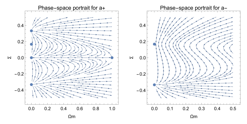
Figure 1: Phase-space portraits for the two-dimensional dynamical system (49), (50) for $\alpha=\alpha_{+}\left(\Omega_{m},\Sigma\right)$ (left figure) and$~{}\alpha=\alpha_{-}\left(\Omega_{m},\Sigma\right)~{}$(right figure).

V.2 Stationary points of the modified Szekeres system

We perform the same analysis for the determination of the stationary points for the modified Szekeres system with the quantum potential term by assuming that $\varepsilon Q_{0}\neq 0$.

V.2.1 Branch $\alpha_{+}$

For the $\alpha_{+}$ branch and for small values of $\varepsilon Q_{0}$, the stationary points are calculated

$$\bar{A}_{1} =\left(1-\varepsilon Q_{0},0\right)~{},~{}\bar{A}_{2}=\left(0,0\right)~{},~{}\bar{A}_{3}=\left(0,-\frac{1}{3}\right)~{},~{}\bar{A}_{4}=\left(0,\frac{1}{3}\left(1-\varepsilon Q_{0}\right)\right)~{},~{}$$ (60)

$$\bar{A}_{5} =\left(0,\frac{1}{6}\right)~{},~{}\bar{A}_{6}=\left(-3,-\frac{1}{3}\right)~{},~{}\bar{A}_{7}=\left(-8+4\varepsilon Q_{0},-\frac{1}{2}+\frac{\varepsilon Q_{0}}{18}\right)\text{. }$$ (61)

Points $\bar{A}_{6},~{}\bar{A}_{7}$ are not physically accepted, while $\bar{A}_{1}$ cannot be accepted because at this stationary solution the condition $\sqrt{\frac{2}{u}}v\rightarrow\infty$ is violated. Therefore, the only stationary solution which is modified is the asymptotic solution of point $\bar{A}_{4}$. The spatial curvature at the point $\bar{A}_{4}$ is derived to be $\Omega_{R}\left(\bar{A}_{4}\right)=-\varepsilon Q_{0}$, from which we infer that the solution at the point describes a Kantowski-Sachs (-like) universe or a Bianchi III (-like) universe for $\varepsilon Q_{0}<0$. However, because $\varepsilon Q_{0}\rightarrow 0$, the solution at the point can be seen as the limit of a Kasner (-like) solution

For the asymptotic solution at the points $\bar{A}_{4}$ we calculate $q\left(\bar{A}_{4}\right)=-1+\frac{4}{3}\varepsilon Q_{0}$. Hence

$$\frac{\dot{\theta}}{\theta^{2}}=-1+\frac{4}{3}\varepsilon Q_{0}\text{~{},~{}}$$ (62)

that is,

$$\theta\left(t\right)=\frac{1}{1-\frac{4}{3}\varepsilon Q_{0}}\frac{1}{\left(t-t_{0}\right)}\simeq\left(1+\frac{4}{3}\varepsilon Q_{0}\right)\frac{1}{\left(t-t_{0}\right)}$$ (63)

while the anisotropic index $\sigma$ is

$$\sigma\left(t\right)\simeq\frac{1}{3}\left(1+\frac{\varepsilon Q_{0}}{3}\right)\frac{1}{\left(t-t_{0}\right)}.$$ (64)

Therefore, the power law indices of the scale factors follow from the algebraic system $p_{1}+2p_{2}=\left(1+\frac{4}{3}\varepsilon Q_{0}\right),~{}\frac{1}{3}\left(p_{1}-p_{2}\right)^{2}=\frac{1}{3}\left(1+\frac{\varepsilon Q_{0}}{3}\right)$which gives

$$\left(p_{1},p_{2}\right)_{A}=\left(-\frac{1}{3}+\frac{\varepsilon Q_{0}}{3},\frac{2}{3}+\frac{\varepsilon Q_{0}}{2}\right)~{},$$ (65)

$$\left(p_{1},p_{2}\right)_{B}=\left(1+\frac{5\varepsilon Q_{0}}{9},\frac{7}{18}\varepsilon Q_{0}\right).$$ (66)

It is clear that the asymptotic solution at point $\bar{A}_{4}$ is not that of vacuum and that a nonzero energy momentum tensor corresponds to that solution. In the $1+3$ decomposition, and for the comoving observer $u^{\mu}=\delta_{t}^{\mu},~{}\$the energy momentum tensor has components

$$T_{\mu\nu}=\mu u_{\mu}u_{\nu}+ph_{\mu\nu}+\pi_{\mu\nu},$$ (67)

where $\mu=T_{\mu\nu}u^{\mu}u^{\nu}~{},~{}p=\frac{1}{3}T_{\mu\nu}h^{\mu\nu}$ and $\pi_{\mu\nu}=T_{\kappa\lambda}\left(h_{\mu}^{\kappa}h_{\nu}^{\lambda}-\frac{1}{3}h^{\kappa\lambda}h_{\mu\nu}\right)$.

Hence, for the power indices $\left(p_{1},p_{2}\right)_{A}$ we calculate

$$\mu_{A}=\frac{7}{9}\frac{\varepsilon Q_{0}}{\left(t-t_{0}\right)^{2}}~{},~{}p_{A}=-\frac{1}{9}\frac{\varepsilon Q_{0}}{\left(t-t_{0}\right)^{2}}~{},$$ (68)

$${}_{A}\pi_{\nu}^{\mu}=diag\left(0,-\frac{26}{27}\frac{\varepsilon Q_{0}}{\left(t-t_{0}\right)^{2}},\frac{10}{27}\frac{\varepsilon Q_{0}}{\left(t-t_{0}\right)^{2}},\frac{10}{27}\frac{\varepsilon Q_{0}}{\left(t-t_{0}\right)^{2}}\right).$$ (69)

Furthermore, for the set of the power indices $\left(p_{1},p_{2}\right)_{B}$ we calculate

$$\mu_{B}=\frac{7}{9}\frac{\varepsilon Q_{0}}{\left(t-t_{0}\right)^{2}}~{},~{}p_{B}=-\frac{1}{9}\frac{\varepsilon Q_{0}}{\left(t-t_{0}\right)^{2}}~{},$$ (70)

$${}_{B}\pi_{\nu}^{\mu}=diag\left(0,\frac{22}{27}\frac{\varepsilon Q_{0}}{\left(t-t_{0}\right)^{2}},-\frac{14}{27}\frac{\varepsilon Q_{0}}{\left(t-t_{0}\right)^{2}},\frac{14}{27}\frac{\varepsilon Q_{0}}{\left(t-t_{0}\right)^{2}}\right).$$ (71)

Recall that in the later solutions $\dot{t}_{0}=0$ holds, but $t_{0}$ is a function of the space variables of the spacetime.

We conclude that a nonzero energy momentum tensor is introduced by quantum corrections in Bohmian mechanics for the Szekeres system. Hence ,the Szekeres system admits semi-classical trajectories which do not remain silent in the quantum level.

As far as the stability of the stationary points is concerned, that remains invariant and it is the same with that of the Szekeres system studied above.

V.2.2 Branch $\alpha_{-}$

For $\alpha=\alpha_{-}\left(\Omega_{m},\Sigma\right)$ we calculate the stationary points

$$\bar{B}_{1} =\left(1-Q_{0},0\right)~{}~{},~{}\bar{B}_{2}=\left(0,-\frac{1}{3}\right)~{},~{}\bar{B}_{3}=\left(0,\frac{1}{6}\right)~{},~{}$$ (72)

$$\bar{B}_{4} =\left(0,\frac{1}{3}\left(1-\varepsilon Q_{0}\right)\right)~{},~{}\bar{B}_{5}=\left(-8+4\varepsilon Q_{0},-\frac{1}{2}+\frac{\varepsilon Q_{0}}{18}\right).$$ (73)

The stationary point $\bar{B}_{5}$ is not physically accepted, while point $\bar{B}_{1}$ violates the condition $\sqrt{\frac{2}{u}}v\rightarrow\infty$ and we do not consider it. Points $\bar{B}_{2}~{}$and $\bar{B}_{3}$ have the same physical properties and stability with points $B_{2},~{}B_{3}$ respectively. $\bar{B}_{4}$ is a new point which has the physical properties of point $\bar{A}_{4}$.

Therefore in the branch $\alpha=\alpha_{-}\left(\Omega_{m},\Sigma\right)$ because of the quantum potential a new stationary point exists. The eigenvalues of the linearized system around the point $\bar{A}_{4}$ are found to be $e\left(\bar{A}_{4}\right)=\left(1-\frac{4}{3}\varepsilon Q_{0},\frac{2}{3}-Q_{0}\varepsilon\right)$ from which we infer that point $\bar{A}_{4}$ is a source and the asymptotic solution at the point is always unstable.

VI Conclusion

In this work we studied the quantization process for the Szekeres system and the effects of the quantum corrections in inhomogeneous cosmological models as they are described by the De Broglie–Bohm theory for quantum mechanics. We make use of previous results and we wrote the Szekeres system in its Hamiltonian equivalent. We calculated the conservation laws for the classical system and we derived previous results while we were able to determine new conservation laws which were not found before. One of these conservation laws is the Lewis invariant which is an important adiabatic invariant for the oscillator with many applications in quantum mechanics. The remaining new conservation laws which we derived exist when the Hamiltonian system is conformally invariant, that is, when the conservation law of the “energy” is identical to zero. That means that these new conservation laws, which are constructed by conformal symmetries of the kinetic metric for the Hamiltonian system, exist for a specific set of trajectories for the classical Szekeres system.

These new conservation laws applied to define differential operators are necessary to quantize the Szekeres system. We found new similarity solutions for the wave function of the Szekeres system. From these new wave functions we were able to constructed a nonzero quantum potential by applying the approach of Bohmian mechanics. In order to understand the effects of the quantum potential term in the original Szekeres system we wrote the modified Szekeres system and we studied the dynamics and the asymptotic solutions, for the trajectories with the initial condition the “energy” of the Hamiltonian equivalent system to be zero.

The main result of this analysis is that because of the quantum correction term, the dynamical evolution of the Szekeres system is modified, such that new asymptotic solutions exist which describe approximately Bianchi I spacetimes which modify the Kasner solutions of the Szekeres systems. These new Bianchi I solutions correspond to exact inhomogeneous solutions with a nonzero anisotropic fluid component with nonzero pressure and stress tensor terms. We conclude that quantum corrections can remove the “silent” property of the Szekeres universe, making the Szekeres model more useful in cosmological studies. Therefore, we show that quantum corrections can be seen as a mechanism to introduce negative pressure term in the cosmological fluid which is interesting since it may have applications for the description of the mechanism which starts the inflationary epoch.

References

- (1) M. Bojowald, Rep. Prog. Phys. 78, 023901 (2015)
- (2) S. Gielen and L. Sindoni, Sigma 12, 082 (2016)
- (3) B.S. DeWitt, Phys. Rev. 160, 1113 (1967)
- (4) J.B. Hartle and S.W. Hawking, Phys. Rev. D 28, 2960 (1983)
- (5) D. Bohm, Phys. Rev. 55, 166 (1952)
- (6) D. Bohm, Phys. Rev. 85, 180 (1952)
- (7) P. Pinto-Neto and R. Colistete Jr., Phys. Lett. A 290, 219 (2001)
- (8) P.A. Terzis, N. Dimakis and T. Christodoulakis, Phys. Rev. D. 90, 123543 (2014)
- (9) F.T. Falciano, N. Pinto-Neto and W. Struyve, Phys. Rev. D 91 043524 (2015)
- (10) A. Krasiński, Inhomogeneous Cosmological Models, Cambridge U.P., Cambridge, (1997)
- (11) R. Easther, L.C. Price and J. Rasero, JCAP 08, 041 (2014)
- (12) T. Buchert and N. Obadia, Class. Quantum Grav. 28, 162002 (2011)
- (13) K. Clough, E.A. Lim, B.S. DiNunno, W. Fischler, R. Flauger and S. Pabah, JCAP 09, 025 (2017)
- (14) M.C.D. Marsh, J.D. Barrow and C. Ganguly, JCAP 05, 026 (2018)
- (15) T. Chiba, Phys. Rev. D 59, 083508 (1999)
- (16) C. Saulder, S. Mieske, E. van Kampen and W.W. Zeilinger, A&A 622, A83 (2019)
- (17) C. Clarkson and M. Regis, JCAP 02, 013 (2011)
- (18) K. Bolejko, Gen. Rel. Grav. 41, 1737 (2009)
- (19) K. Bolejko and M. Korzyński, IJMPD 26, 1730011 (2017)
- (20) A.E. Romano, IJMPD 21, 1250085 (2012)
- (21) P. Szekeres, Commun. Math. Phys. 41, 55 (1975)
- (22) N. Mustapha, G.F.R. Ellis, H. van Elst and M. Marklund, Class. Quantum Gravit. 17, 3135 (2000)
- (23) M. Bruni, S. Matarrese and P. Ornella, Astro. J. 445, 958 (1995)
- (24) K. Bolejko and M.-N. Celerier, Phys. Rev. D 82, 103510 (2010)
- (25) K. Bolejko, Gen. Relativ. Grav. 41, 1737 (2009)
- (26) M. Ishak and A. Peel, Phys. Rev. D 85, 083502 (2012)
- (27) D. Vrba and O. Svitek, Gen. Relativ. Grav. 46, 1808 (2014)
- (28) W.B. Bonnor, MNRAS 167, 55 (1974)
- (29) W.B. Bonnor, MNRAS 175, 85 (1976)
- (30) K. Bolejko, W.R. Stoeger, Gen. Relat. Gravit. 42, 2349 (2010)
- (31) D.A. Szafron, J. Math. Phys. 18, 1673 (1977)
- (32) J.D. Barrow and J. Stein-Schabes, Phys. Lett. A 103, 315 (1984)
- (33) S.W. Goode and J. Wainwright, Gen. Relativ. Gravit. 18, 315 (1986)
- (34) N. Tomimura, Nuovo Cimento B 42, 1 (1977)
- (35) J.D. Barrow and A. Paliathanasis, EPJC 78, 767 (2018)
- (36) J.D. Barrow and A. Paliathanasis, Cyclic Szekeres Universes, EPJC 79, 379 (2019)
- (37) A. Paliathanasis, G. Leon and J.D. Barrow, EPJC 80, 731 (2020)
- (38) R. Maartens, W. Lesame and G.F.R. Ellis, Phys.Rev. D 55, 5219 (1997)
- (39) A. Paliathanasis and P.G.L. Leach, Phys. Lett. A 381, 1277 (2017)
- (40) A. Gierzkiewicz and Z.A. Golda, J. Nonl. Math. Phys. 24, 494 (2016)
- (41) J. Llibre and C. Valls, Phys. Lett. A 383, 301 (2019)
- (42) A. Paliathanasis, A. Zampeli, T. Christodoulakis and M.T. Mustafa, Class. Quantum Grav. 35, 125005 (2018)
- (43) A. Zampelia and A. Paliathanasis, Quantization of inhomogeneous spacetimes with cosmological constant term, (2020) [arXiv:2012.10814]
- (44) T. Christodoulakis, N. Dimakis, P.A Terzis and G. Doulis, Phys. Rev. D 90, 024052 (2014)
- (45) A. Paliathanasis, EPJC 79, 1031 (2019)
- (46) A. Paliathanasis, M. Tsamparlis, S. Basilakos and J.D. Barrow, Phys. Rev. D 93, 043528 (2016)
- (47) M. Lutzky, Phys. Lett. A 68, 3 (1978)
- (48) H.R. Lewis Jr. J. Math. Phys. 9, 1976 (1968)
- (49) M. Kruskal, J. Math. Phys. 3, 806 (1962)
- (50) P.G.L. Leach, Siam J. Appl. Math. 34, 496 (1978)
- (51) J.R. Ray and J.L. Reid, Phys. Lett. A 71, 317 (1979)
- (52) R.M. Hawkins and J.E. Lidsey, Phys. Rev. D 66, 023523 (2002)
- (53) M. Tsamparlis and A. Paliathanasis, Symmetry 10, 233 (2018)
- (54) M. Tsamparlis, A. Paliathanasis, S. Basilakos and S. Capozziello, Gen. Rel. Grav. 45, 2003 (2013)
- (55) T. Christodoulakis, N. Dimakis and P.A. Terzis, J. Phys. A: Math. Theor. 47, 095202 (2014)
- (56) P.A. Terzis, N. Dimakis, T. Christodoulakis, A. Paliathanasis and M. Tsamparlis, J. Geom. Phys. 101, 52 (2016)
- (57) I. Bialynicki-Birula, M. Cieplak and J. Kaminski, Theory of Quanta, Oxford University Press, Oxford (1992)