Gravitational waves from Population III binary black holes are consistent with LIGO/Virgo O3a data for the chirp mass larger than $\sim 20{M}_{\odot}$

Abstract

The probability number distribution function of binary black hole mergers observed by LIGO/Virgo O3a has double peaks as a function of chirp mass $M_{\rm chirp}$, total mass $M_{\rm total}$, primary black hole mass $M_{1}$ and secondary one $M_{2}$, respectively. The larger chirp mass peak is at $M_{\rm chirp}\cong 30{M}_{\odot}$. The distribution of $M_{2}$ vs. $M_{1}$ follows the relation of $M_{2}\cong 0.7M_{1}$. For initial mass functions of Population III stars in the form of $f(M)\propto M^{-\alpha}$, population synthesis numerical simulations with $0\leq\alpha\leq 1.5$ are consistent with O3a data for $M_{\rm chirp}\gtrsim 20{M}_{\odot}$. The distribution of $M_{2}$ vs. $M_{1}$ for simulation data also agrees with $M_{2}\cong 0.7M_{1}$ relation of O3a data.

1 Introduction

The second LIGO–Virgo Gravitational-Wave Transient Catalog (GWTC-2) was announced on October 28, 2020 (Abbott et al., 2020). In a companion paper (The LIGO Scientific Collaboration et al., 2020), population properties of compact object binaries observed during the first half of the third observing run (O3a) have been discussed, especially by focusing on the primary mass and spin distributions for BBHs (Binary Black Holes). Specifically, they analysed the merger rate density distribution as a function of primary mass $M_{1}$, and showed that the power law + peak model is the most likely one. Figure 1 plots the power law + peak model with BH mass distribution of Population (Pop) I/II BH (Belczynski et al., 2020) and Pop III BH (Kinugawa et al., 2020). The power law + peak model looks like consistent with the power law mass distribution of Pop I/II BHs (Belczynski et al., 2020) and the mass distribution of Pop III BHs with the peak at $\sim 30$–$40{M}_{\odot}$ (Kinugawa et al., 2020). Since Figure 1 is shown as a function of the primary mass $M_{1}$, it is also important to study the merger rate as functions of secondary mass $M_{2}$, total mass $M_{\rm total}$ and chirp mass $M_{\rm chirp}$ in order to check whether the Pop III BH model is consistent with the peak of massive BBHs or not, varying IMF (Initial Mass Function) and SFR (Star Formation Rate).

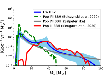
Figure 1: BBH merger rate density as a function of primary mass ($M_{1}$). The blue line and the light blue region are the population distribution and 90% credible interval of the power law + peak model by GWTC-2, respectively (The LIGO Scientific Collaboration et al., 2020). The green dashed line is the Pop I/II BBH merger rate density of the M30.B model in Belczynski et al. (2020). The gray line is the Salpeter like power law model ($M_{1}^{-2.35}$) for Pop I/II BBHs which is normalized by GWTC-2 rate at $M_{1}=10{M}_{\odot}$. The red line shows the Pop III BBH merger rate density of the M100 model in Kinugawa et al. (2020) which is the same as the flat model in this paper.

In this Letter, firstly, we focus on the chirp mass distribution of BBHs because the chirp mass is the most sensitive parameter in GW observation of compact object binaries where the chirp mass ($M_{\rm chirp}$) is defined by $M_{\rm chirp}=(M_{1}M_{2})^{3/5}/(M_{1}+M_{2})^{1/5}$. Secondly, we omit binaries which include a compact object with mass $<3{M}_{\odot}$, i.e., GW190425 ($M_{1}=2{M}_{\odot}$, $M_{2}=1.4{M}_{\odot}$), GW190426_152155 ($M_{1}=5.7{M}_{\odot}$, $M_{2}=1.5{M}_{\odot}$) and GW190814 ($M_{1}=23.2{M}_{\odot}$, $M_{2}=2.59{M}_{\odot}$) in the 39 GW events in GWTC-2 O3a so that we consider 36 GW events only. Thirdly, we do not treat spins of BBHs although there are interesting results related to the BH spins (Fragione & Loeb, 2021; Callister et al., 2020; Gerosa et al., 2020; Trani et al., 2021). This is because there are still large uncertainties in the estimation of BH spins.

After the announcement of GWTC-2, various interesting papers have been presented; Antonini & Gieles (2020) found a drop in the BBH merger rate for $M_{1}\lesssim 13$ and $\gtrsim 30{M}_{\odot}$ in a population synthesis code of BBH formation in globular clusters (GCs) with a wide set of initial conditions (note that hierarchical mergers to create heavier primary mass BHs are only $\lesssim 10\%$ of the total number of BBH mergers expected from GCs (Rodriguez et al., 2018, 2019)), Tiwari & Fairhurst (2020) reanalyzed GWTC-2 for the chirp mass, mass ratio, and spin distributions with minimal assumptions (Tiwari, 2020) and found peaks in the chirp mass distribution at $8$, $14$, $26$, and $45{M}_{\odot}$, Kimball et al. (2020a) presented that GWTC-2 is best modelled with hierarchical formation channels by using a phenomenological population model (Kimball et al., 2020b) based on simulations of metal-poor GCs (Rodriguez et al., 2019) (note that GWTC-1 (Abbott et al., 2019) was consistent with having no hierarchical merger in this model), Veske et al. (2021) gave a search for hierarchical triple mergers including spin effects, and analyzed the GW events by assuming upper bounds on the mass distribution of first generation BHs, and Fishbach et al. (2021) paid attention to the absence of BBH events with $M_{1}>45{M}_{\odot}$ at low redshifts, and discussed the evolution of the BBH mass distribution that will be distinguishable in future GW observations. Banerjee (2020a) obtained BBH merger rate densities and differential BBH merger rate densities which are consistent with the LIGO–Virgo result, for dynamical BBH formation in young massive star clusters and open star clusters based on N-body evolutionary models of star clusters including hierarchical mergers (Banerjee, 2020b). Although Rodriguez et al. (2021) showed that the redshift-dependent merger rate of GWTC-2 can be explained by a purely dynamical origin in GCs, they cautioned that various formation scenarios could contribute the rate. In practice, Wong et al. (2020b); Zevin et al. (2020); Bouffanais et al. (2021) have considered mixture models by introducing hyper-parameters to describe the fraction of each formation channel. We also see scenarios with primordial BHs (PBHs) formed in the early Universe; Wong et al. (2020a) introduced a PBH scenario with accretion to explain the presence of several spinning BBHs in GWTC-2, Deng (2021) discussed a possible mass distribution of primordial black holes by assuming that all LIGO/Virgo BBHs have a primordial origin, and Hütsi et al. (2020); De Luca et al. (2021) considered combination of populations of astrophysical BHs and PBHs (see also Hall et al. (2020) for GWTC-1).

Pop III BHs are not included in any analysis of BBH formation models mentioned above, although the Pop III binaries are considered as a candidate of the massive BBH origin (e.g. Kinugawa et al., 2014, 2020, 2021a; Tanikawa et al., 2020; Farrell et al., 2020). We believe that we can add one more interesting paper on the O3a events.

2 Analysis

2.1 Data from LIGO/Virgo GWTC-2 O3a

Using the median values and 90% credible intervals of parameters estimated by Abbott et al. (2020), we prepare a simple probability number distribution function of various mass ‘$m$’ to introduce the parameter estimation errors as

$$g(m)= (2\pi\sigma_{-}^{2})^{-1/2}\exp\left\{-\frac{(m-m_{0})^{2}}{2\sigma_{-}^{2}}\right\}\Theta(m_{0}-m)$$ (1)

$$+(2\pi\sigma_{+}^{2})^{-1/2}\exp\left\{-\frac{(m-m_{0})^{2}}{2\sigma_{+}^{2}}\right\}\Theta(m-m_{0})\,,$$ (2)

where each side of $m=m_{0}$ has 50% probability, i.e., $m_{0}$ is the median, and $\sigma_{-}$ and $\sigma_{+}$ are determined from the 90% credible interval.

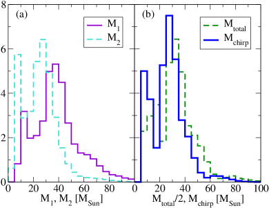
Figure 2: Probability number distributions of primary ($M_{1}$ in (a)), secondary ($M_{2}$ in (a)), total ($M_{\rm total}$ in (b)), and chirp ($M_{\rm chirp}$ in (b)) masses of the observed 36 BBHs by using the GWTC-2 data (Abbott et al., 2020). The lines correspond to the probability number of stars in the mass interval of $5{M}_{\odot}$. Note that the horizontal axis for the total mass is $M_{\rm total}/2$.

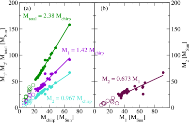
Figure 3: Distribution of median values of various masses; $M_{1}$ vs. $M_{\rm chirp}$, $M_{2}$ vs. $M_{\rm chirp}$, and $M_{\rm total}$ vs. $M_{\rm chirp}$ in (a), and $M_{2}$ vs. $M_{1}$ in (b). The circles and filled circles show BBHs with chirp mass lower or higher than $20{M}_{\odot}$, respectively. Each straight line shows the best fitting one for $M_{\rm chirp}>20{M}_{\odot}$.

The probability number distributions of primary ($M_{1}$), secondary ($M_{2}$), total ($M_{\rm total}$), and chirp ($M_{\rm chirp}$) masses for the 36 BBHs are shown in Figure 2 (a) and (b) where the horizontal axis is shown in unit of ${M}_{\odot}$ while the lines correspond to the probability number of stars in the mass interval of $5{M}_{\odot}$. Note that we use $M_{\rm total}/2$ for the total mass in Figure 2 (b). In all distributions, we can identify double peaks of probability number of stars. We confirmed that they exist even for the case with the mass interval of $2.5{M}_{\odot}$. The higher peaks of various mass are at $\sim 46{M}_{\odot}$, $\sim 32{M}_{\odot}$, $\sim 77{M}_{\odot}$ and $\sim 32{M}_{\odot}$ for $M_{1}$, $M_{2}$, $M_{\rm total}$ and $M_{\rm chirp}$, respectively, while the lower peaks are at $\sim 18{M}_{\odot}$, $\sim 10{M}_{\odot}$, $\sim 28{M}_{\odot}$ and $\sim 11{M}_{\odot}$ for $M_{1}$, $M_{2}$, $M_{\rm total}$ and $M_{\rm chirp}$, respectively.

In Figure 3 (a), taking the median value of $M_{\rm chirp}$ as the horizontal axis, we plot the median value of $M_{1}$, $M_{2}$ and $M_{\rm total}$ for each event, respectively. Here, the 10 circles and 26 filled circles show BBHs with $M_{\rm chirp}$ lower and higher than $20{M}_{\odot}$, respectively. We also show the median values of $M_{2}$ vs. $M_{1}$ in Figure 3 (b) where we use the value of $M_{\rm chirp}$ but not the value of $M_{1}$ and $M_{2}$ to determine if a certain point in the figure is a circle or a filled circle. From Figure 3 (a) and Figure 2 (a) and (b), we can identify two groups of BBHs in the distributions of $M_{1}$, $M_{2}$ and $M_{\rm total}$ as a function of $M_{\rm chirp}$. The boundary of two groups is at $M_{\rm chirp}\sim 20{M}_{\odot}$. The lines in Figure 3 (a) and (b) are the best linear fitting ones for $M_{\rm chirp}>20{M}_{\odot}$. They are $M_{1}=1.42M_{\rm chirp}$, $M_{2}=0.967M_{\rm chirp}$, $M_{\rm total}=2.38M_{\rm chirp}$ and $M_{2}=0.673M_{1}$, respectively. The correlation coefficients for each distribution are $0.957$, $0.978$, $0.996$ and $0.875$, respectively. Since these are good correlations, there should be some physical explanations for them.

We assume first that the correlation between $M_{1}$ and $M_{2}$ is given as $M_{2}=0.673M_{1}$ from Figure 3 (b). From the definition of the chirp mass and $M_{2}=0.673M_{1}$, we have $M_{1}=1.41M_{\rm chirp}$, $M_{2}=0.946M_{\rm chirp}$ and $M_{\rm total}=2.35M_{\rm chirp}$ which agree quite well with $M_{1}=1.42M_{\rm chirp}$, $M_{2}=0.967M_{\rm chirp}$, $M_{\rm total}=2.38M_{\rm chirp}$ obtained from Figure 3 (a), respectively. This means that the relation of $M_{2}=0.673M_{1}$ is the most important one, and thus other three relations are obtained from this $M_{2}=0.673M_{1}$ relation.

What is the physical origin of the relation of $M_{2}=0.673M_{1}$? We first notice that the smallest mass ratio $q~{}(=M_{2}/M_{1})$ of 36 BBHs observed in O3a is $\gtrsim 0.3$ (The LIGO Scientific Collaboration et al., 2020) while in population synthesis models of Pop III stars such as in Kinugawa et al. (2014), the initial mass ratio $q$ of binaries ranges from $10{M}_{\odot}/M_{1}$ to $1$. Therefore, binaries with small mass ratio of $q<0.3$ exist when the binaries are first formed. However, the binaries with such small mass ratio tend to have large mass ratio due to mass transfer so that the fraction of merging Pop III BBH with $q\lesssim 0.5$ is much smaller than that of $q>0.5$ (Kinugawa et al., 2016b). In reality, most of the binary events in GWTC-2 satisfy $0.6<q<0.8$ from Figure 3 (b). Therefore, the relation of $M_{2}=0.673M_{1}$ is consistent with Pop III star origin.

In Figure 4, the median values of secondary mass for each primary mass of Pop III BBHs which merge within the Hubble time are shown for various models. Although details of various population synthesis simulation models of Pop III BBHs are described in the next section, one can identify $M_{2}\cong 0.7M_{1}$ relation similar to Figure 3 (b) for various models up to $M_{1}\sim 50{M}_{\odot}$. On the other hand, in the cases of Pop I/II field binaries and dynamical formation in dense star clusters, we estimate the median values of secondary mass using Figure 26 in Belczynski et al. (2020) and Figure 6 in Rodriguez et al. (2019). They follow the relations of $M_{2}\sim 0.8M_{1}$, and $M_{2}\sim 0.87M_{1}$, respectively. The values of $M_{2}/M_{1}$ of these relations are lager than those of the O3a observation and Pop III BBH simulations. Especially, in the case of the dynamical formation, the mass ratio is much larger than those of Pop I/II and Pop III cases. The reason for this difference seems to come from repeated dynamical encounters, by which many exchanges of BHs make the binary to be a nearly equal-mass system although BBH was born with low mass ratio.

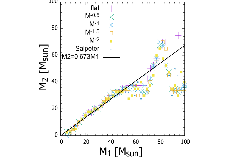
Figure 4: $M_{2}$ vs. $M_{1}$ of the BBHs which merge within the Hubble time, for various population synthesis simulation models of Pop III origin BBHs with IMF such as flat, $M^{-0.5},M^{-1},M^{-1.5},M^{-2}$ and $M^{-2.35}$ (Salpeter), respectively. The mean values of median value of secondary mass $M_{2}$ for each primary mass $M_{1}$ are plotted. $M_{2}\cong 0.7M_{1}$ relation can be seen for all models up to $M_{1}\sim 50{M}_{\odot}$ similar to Figure 3 (b). For details of the simulations, see Section 2.2.

2.2 Results from population synthesis of Pop III binaries

To calculate the number of events from the population synthesis simulations, we need the observable distance (redshift) for each binary. Here, we treat only nonspinning equal-mass binaries to calculate the maximum observable redshift $z_{\rm max}$ for the LIGO O3a-Livingston (O3a-L) by using the inspiral–merger–ringdown waveform shown in Nakamura et al. (2016); Nakano et al. (2021) (see also Kinugawa et al. (2021b) for the O3a-L sensitivity curve).

For simplicity, we calculate the sky and polarization averaged SNR (Signal-to-Noise Ratio), and treat the chirp mass and redshift (where the luminosity distance, $D_{L}$ is a function of $z$) as the parameters of the waveform. Although SNR also depends on the mass ratio, we confirm for the O3a-L sensitivity that the difference is at most $\sim 20\%$ in the estimation of luminosity distance for binaries with redshifted chirp mass $(1+z)M_{\rm chirp}=5$–$126{M}_{\odot}$ in the case of $1/3\leq q\leq 1$. This means that we consider $M_{\rm chirp}=5$–$70{M}_{\odot}$ at $z\leq 0.8$. For a BBH with a redshifted chirp mass, the SNR difference is related to the difference in the luminosity distance directly, i.e., $D_{L}\propto 1/{\rm SNR}$. This difference due to the assumption of equal-mass binaries is much smaller than errors ($\sim 300\%$) in the LIGO/Virgo estimation of luminosity distances (Abbott et al., 2020). In the above assumption, the maximum observable redshift $z_{\rm max}$ for BBHs with various $M_{\rm chirp}$ by setting the averaged SNR $=8$ for O3a-L is obtained as Figure 5 and can be expressed by a fitting function as

$$z_{\rm max}= 0.01319\,\frac{M_{\rm chirp}}{{M}_{\odot}}-7.453\times 10^{-6}\,\left(\frac{M_{\rm chirp}}{{M}_{\odot}}\right)^{2}$$ (3)

$$-4.332\times 10^{-7}\,\left(\frac{M_{\rm chirp}}{{M}_{\odot}}\right)^{3}\,.$$ (4)

Note that when we apply the fitting functions shown in Figure 3 to evaluate the maximum observable redshift, the error in the maximum redshift due to the equal-mass assumption is only $\sim 3\%$.

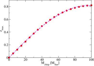
Figure 5: Maximum observable redshift $z_{\rm max}$ obtained by setting the averaged SNR $=8$ for nonspinning equal-mass BBHs with various $M_{\rm chirp}$ for the LIGO O3a-Livingston (O3a-L) sensitivity. The dashed (magenta) curve is the fitting shown in Eq. (4).

We simulate $10^{6}$ Pop III binary evolutions using the binary population synthesis code (Kinugawa et al., 2014, 2020). In this Letter, $10$–$100{M}_{\odot}$ Pop III stellar evolutions are discussed because of the following two reasons. First, the typical mass of Pop III stars is considered to be several tens solar mass (e.g. Hosokawa et al., 2011; Hirano et al., 2014; Susa et al., 2014; Tarumi et al., 2020). Second, the observed BH masses with mass $\lesssim 80{M}_{\odot}$, can be explained by Pop III stars with initial mass $<100{M}_{\odot}$ (Kinugawa et al., 2020).

We treat 6 IMF models: flat, $M^{-0.5}$, $M^{-1}$, $M^{-1.5}$, $M^{-2}$, and Salpeter ($M^{-2.35}$) IMFs. The flat model in this Letter is the same as M100 model in Kinugawa et al. (2020). In other models, we use the same initial distribution functions and binary parameters as those of the flat model except for IMF. As for SFR as a function of the redshift $z$, we use that of de Souza et al. (2011) with a factor of three smaller rate to be consistent with the restriction from CMB data by Planck (Visbal et al., 2015; Inayoshi et al., 2016).

Let us first define $R_{a,m}(t)$ as the merger rate density for individual mass ‘$m$’ of the binary per co-moving volume at the cosmological time $t$ for a certain model ‘$a$’ such as Pop III BBHs. Using Eq. (90) in Kinugawa et al. (2014), $R_{a,m}(t)$ is given by

$$R_{a,m}(t)=\int_{0}^{t}f_{b}\frac{{\rm SFR}(t^{\prime})}{\langle M\rangle}\frac{N_{a,m}(t-t^{\prime})}{N_{\rm tot}}dt^{\prime}\,,$$ (5)

where $f_{b}$, ${\rm SFR}(t)$, $\langle M\rangle$, $N_{a,m}(t-t^{\prime})\,dt^{\prime}$ and $N_{\rm tot}$ are the fraction of the total number of binaries to that of stars, SFR per co-moving volume per cosmic time, mean mass of the stars, the number of Pop III BBH merger events during $dt^{\prime}$ for individual mass ‘$m$’ with a delay time $t-t^{\prime}$ in a certain model ‘$a$’, and the total number of Pop III binaries in the population synthesis simulation, respectively. The physical meaning of the above equation is as follows. First, because $f_{b}$=(the number of binary stars)/(the number of stars), the maximum value of $f_{b}$ is $1/2$ while the fiducial value is $1/3$, which means that $1/3$ of stars is a single star while $2/3$ is a binary. Second, $\rm{SFR}(t^{\prime})/\langle M\rangle$ is the formation rate of the star in number. We use the total mass density of Pop III stars is $\rho_{*,III}=6\times 10^{5}~{}{M}_{\odot}\rm~{}Mpc^{-3}$ (Inayoshi et al., 2016). We assume that the redshift dependence of Pop III SFR is the same as the Pop III SFR of de Souza et al. (2011). Finally, $N_{a,m}(t-t^{\prime})/N_{\rm tot}$ gives the fraction of the Pop III BBH mergers with a delay time $t-t^{\prime}$ for individual mass ‘$m$’ in model ‘$a$’.

Using Eq. (94) in Kinugawa et al. (2014), we obtain the expected number of events in time interval of $\Delta t$ up to the redshift $z$ for individual mass ‘$m$’ by

$$n_{a,m}(z)=4\pi\int_{0}^{z}R_{a,m}(z^{\prime})[r(z^{\prime})]^{2}\frac{1}{1+z^{\prime}}\frac{dr(z^{\prime})}{dz^{\prime}}dz^{\prime}\times\Delta t\,,$$ (6)

where $R_{a,m}(z)$ is given by using not ‘$t$’ but ‘$z$’ as an independent variable, $\Delta t=184/365.25$ yr is the observing time of O3a run assuming 100% duty cycle, and $r(z)$ is the co-moving distance given by $r(z)=(c/H_{0})\int_{0}^{z}dz^{\prime}[\Omega_{\rm m}(1+z^{\prime})^{3}+\Omega_{\rm\Lambda}]^{-1/2}$ where we use $H_{0}=67.74\,{\rm km\,s^{-1}\,Mpc^{-1}}$, $\Omega_{\rm m}=0.3089$ and $\Omega_{\rm\Lambda}=1-\Omega_{\rm m}$ from Planck Collaboration et al. (2016). In Eq. (6), we set $z=z_{\rm max}$ evaluated by Eq. (4) with the chirp mass of each BBH under the assumption of equal mass binaries.

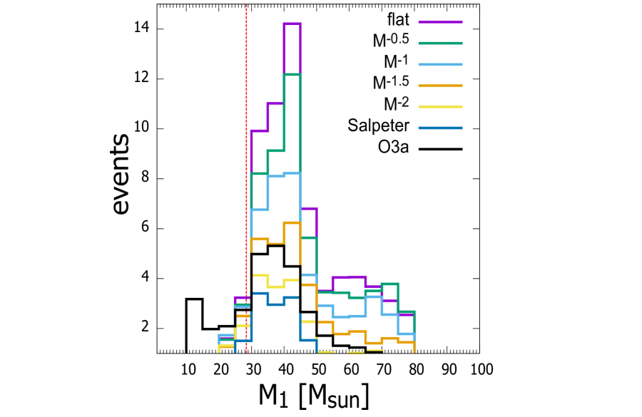
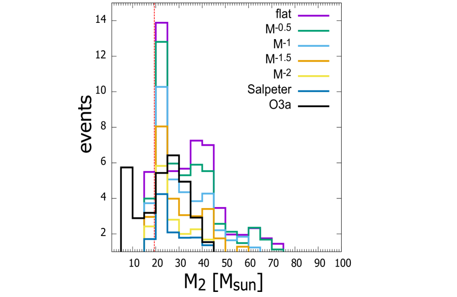
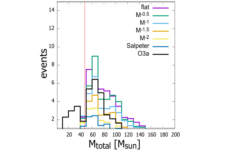
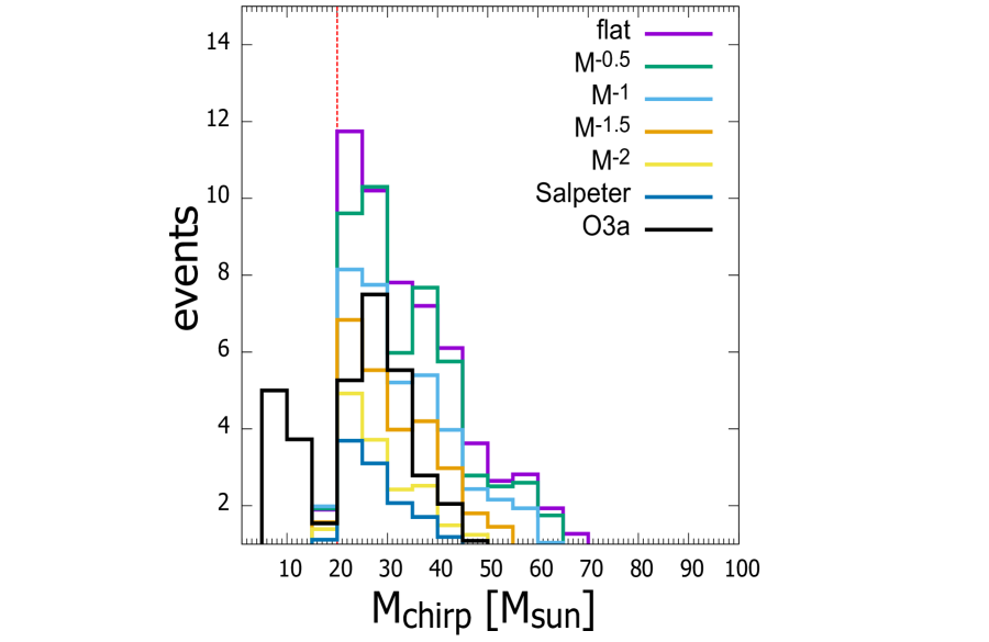
Figure 6: Four kinds of mass, ($M_{1}$, $M_{2}$, $M_{\rm total}$ and $M_{\rm chirp}$), distribution of the number of events during the O3a observation time by the population synthesis simulations of Pop III BBHs using Eq. (6) for various theoretical models of IMF. The purple, green, blue, magenta, yellow and navy lines show the estimation for the flat, $M^{-0.5}$, $M^{-1}$, $M^{-1.5}$, $M^{-2}$ and Salpeter ($M^{-2.35}$) IMFs, respectively. The black lines denote the O3a observation shown in Figure 2. The red vertical dotted lines correspond to $M_{\rm chirp}=20{M}_{\odot}$.

Table 1: Estimation of the minimum $\delta$ calculated by using Eq. (7) for $M_{\rm chirp},M_{1},M_{2}$ and $M_{\rm total}$ and the best fit value of the constant $\lambda$ shown in the parenthesis, respectively. We treat only the range of chirp mass of $20\,{M}_{\odot}\leq M_{\rm chirp}\leq 100\,{M}_{\odot}$ and related ranges derived from the fitting functions shown in Figure 3 for the other masses. Here, $\lambda\leq 1.0$ since we assume $f_{b}=1/3$. The boldface number shows the minimum value of $\delta$ for $M_{\rm chirp}$, $M_{1}$, $M_{2}$ and $M_{\rm total}$, respectively.

Value of $\delta~{}(\lambda)$	flat	$M^{-0.5}$	$M^{-1}$	$M^{-1.5}$	$M^{-2}$	Salpeter ($M^{-2.35}$)
$M_{\rm chirp}$	13.7 (0.518)	14.72 (0.568)	12.5 (0.734)	13.8 (0.950)	24.9 (1.00)	35.8 (1.00)
$M_{1}$	6.54 (0.402)	8.02 (0.465)	4.38 (0.611)	3.22 (0.821)	5.45 (1.00)	14.7 (1.00)
$M_{2}$	27.5 (0.463)	23.0 (0.533)	20.3 (0.678)	20.7 (0.875)	23.3 (1.00)	33.9 (1.00)
$M_{\rm total}$	7.59 (0.654)	10.9 ( 0.710)	9.59 (0.919)	12.1 (1.00)	26.3 (1.00)	42.0 (1.00)

Figure 6 shows four kinds of mass ($M_{1}$, $M_{2}$, $M_{\rm total}$ and $M_{\rm chirp}$) distribution of the number of events during the O3a observation time by the population synthesis simulations of Pop III BBHs using Eq. (6) for various theoretical models of IMF. The red vertical dotted lines correspond to $M_{\rm chirp}=20{M}_{\odot}$. The purple, green, blue, magenta, yellow and navy lines show the estimation for the flat, $M^{-0.5}$, $M^{-1}$, $M^{-1.5}$, $M^{-2}$ and Salpeter ($M^{-2.35}$) IMFs, respectively. To determine which model is the best to explain the mass distributions of O3a data, we compare the value of $\delta$ defined by

$$\delta=\sum_{i}(\lambda n_{i}^{\rm model}-n_{i}^{\rm O3a})^{2}\,,$$ (7)

where $i$ is the number of each mass bin while $n_{i}^{\rm O3a}$ and $n_{i}^{\rm model}$ are presented in Figures 2 and 6, respectively. Using Eq. (7), we minimize $\delta$ as a function of $\lambda$.

In Eq. (7), we have introduced a variable $\lambda$ to fix SFR $\times f_{b}$ of the model. Here, assuming the fiducial value $f_{b}=1/3$, we restrict $\lambda\leq 1.0$. In Table 1, we show estimation of the minimum $\delta$ calculated by using Eq. (7) for $M_{\rm chirp}$, $M_{1}$, $M_{2}$ and $M_{\rm total}$ and the best fit value of the constant $\lambda$ shown in the parenthesis, respectively. Here, $\lambda=0.734$, for example, means the model with 73.4% of star formation rate compared with the fiducial one. We treat only the range of chirp mass of $20\,{M}_{\odot}\leq M_{\rm chirp}\leq 100\,{M}_{\odot}$ and related ranges derived from the fitting functions shown in Figure 3 for the other mass. The boldface number shows the minimum value of $\delta$ for $M_{\rm chirp}$, $M_{1}$, $M_{2}$ and $M_{\rm total}$, respectively. Since the best IMF is not the same for $M_{\rm chirp}$, $M_{1}$, $M_{2}$ and $M_{\rm total}$, we can only state that $0\leq\alpha\leq 1.5$ is preferred from the O3a data.

From Table 1, in the cases of $M_{chirp}$ and $M_{2}$, the minima of $\delta$ are at $\alpha=1$. On the other hand, in the case of $M_{1}$, there are two local minima at $\alpha=0$, and $1.5$, although the global minimum $\delta$ is at $\alpha=1.5$. Furthermore, in the case of $M_{\rm total}$, there are also two local minima at $\alpha=0$, and $1$, although the global minimum of $\delta$ is at $\alpha=0$. To make the situation here clearer, we show in Figure 7 the number distribution of $M_{1}$ with the minimized value of $\lambda$ for each $\alpha$ of IMF. We see that although the fraction of massive BH slightly increases as $\alpha$ decreases, the mass distributions are almost the same for $0\leq\alpha\leq 1.5$. The difference is too small to narrow down the candidates using O3a events. We need more data than those of O3a in order to say which IMF is the best. Our previous works (e.g. Kinugawa et al., 2016a, 2020) show that although the property of Pop III mass distribution hardly depends on binary parameters and initial distributions, the merger rate would change by a factor of a few. Thus, $\lambda$ should depend on binary parameters and initial distributions.

In conclusion, our population synthesis simulations of Pop III stars show that for $M_{\rm chirp}>20{M}_{\odot}$, four kinds of BH masses, i.e., $M_{1}$, $M_{2}$, $M_{\rm total}$ and $M_{\rm chirp}$, distributions of O3a data are consistent with a moderately decreasing IMF in the form of $f(M)\propto M^{-\alpha}$ with $0\leq\alpha\leq 1.5$. The distribution of $M_{1}$ and $M_{2}$ of simulation data agrees with $M_{2}\cong 0.7M_{1}$ relation from O3a.

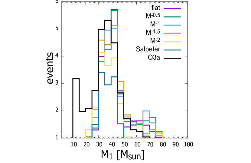
Figure 7: $M_{1}$ distribution for each IMF with the best value of $\lambda$ in Table 1.

Data Availability

Results will be shared on reasonable request to corresponding author.

References

- Abbott et al. (2019) Abbott B. P., et al., 2019, Physical Review X, 9, 031040
- Abbott et al. (2020) Abbott R., et al., 2020, arXiv e-prints, p. arXiv:2010.14527
- Antonini & Gieles (2020) Antonini F., Gieles M., 2020, Phys. Rev. D, 102, 123016
- Banerjee (2020a) Banerjee S., 2020a, arXiv e-prints, p. arXiv:2011.07000
- Banerjee (2020b) Banerjee S., 2020b, MNRAS, 500, 3002
- Belczynski et al. (2020) Belczynski K., et al., 2020, A&A, 636, A104
- Bouffanais et al. (2021) Bouffanais Y., Mapelli M., Santoliquido F., Giacobbo N., Di Carlo U. N., Rastello S., Artale M. C., Iorio G., 2021, arXiv e-prints, p. arXiv:2102.12495
- Callister et al. (2020) Callister T. A., Farr W. M., Renzo M., 2020, arXiv e-prints, p. arXiv:2011.09570
- De Luca et al. (2021) De Luca V., Franciolini G., Pani P., Riotto A., 2021, arXiv e-prints, p. arXiv:2102.03809
- Deng (2021) Deng H., 2021, arXiv e-prints, p. arXiv:2101.11098
- Farrell et al. (2020) Farrell E. J., Groh J. H., Hirschi R., Murphy L., Kaiser E., Ekström S., Georgy C., Meynet G., 2020, arXiv e-prints, p. arXiv:2009.06585
- Fishbach et al. (2021) Fishbach M., et al., 2021, arXiv e-prints, p. arXiv:2101.07699
- Fragione & Loeb (2021) Fragione G., Loeb A., 2021, MNRAS,
- Gerosa et al. (2020) Gerosa D., Mould M., Gangardt D., Schmidt P., Pratten G., Thomas L. M., 2020, arXiv e-prints, p. arXiv:2011.11948
- Hall et al. (2020) Hall A., Gow A. D., Byrnes C. T., 2020, Phys. Rev. D, 102, 123524
- Hirano et al. (2014) Hirano S., Hosokawa T., Yoshida N., Umeda H., Omukai K., Chiaki G., Yorke H. W., 2014, ApJ, 781, 60
- Hosokawa et al. (2011) Hosokawa T., Omukai K., Yoshida N., Yorke H. W., 2011, Science, 334, 1250
- Hütsi et al. (2020) Hütsi G., Raidal M., Vaskonen V., Veermäe H., 2020, arXiv e-prints, p. arXiv:2012.02786
- Inayoshi et al. (2016) Inayoshi K., Kashiyama K., Visbal E., Haiman Z., 2016, MNRAS, 461, 2722
- Kimball et al. (2020a) Kimball C., et al., 2020a, arXiv e-prints, p. arXiv:2011.05332
- Kimball et al. (2020b) Kimball C., Talbot C., Berry C. P. L., Carney M., Zevin M., Thrane E., Kalogera V., 2020b, ApJ, 900, 177
- Kinugawa et al. (2014) Kinugawa T., Inayoshi K., Hotokezaka K., Nakauchi D., Nakamura T., 2014, MNRAS, 442, 2963
- Kinugawa et al. (2016a) Kinugawa T., Miyamoto A., Kanda N., Nakamura T., 2016a, MNRAS, 456, 1093
- Kinugawa et al. (2016b) Kinugawa T., Nakano H., Nakamura T., 2016b, Progress of Theoretical and Experimental Physics, 2016, 103E01
- Kinugawa et al. (2020) Kinugawa T., Nakamura T., Nakano H., 2020, MNRAS, 498, 3946
- Kinugawa et al. (2021a) Kinugawa T., Nakamura T., Nakano H., 2021a, MNRAS, 501, L49
- Kinugawa et al. (2021b) Kinugawa T., Nakamura T., Nakano H., 2021b, Progress of Theoretical and Experimental Physics, 2021, 021E01
- Nakamura et al. (2016) Nakamura T., et al., 2016, PTEP, 2016, 093E01
- Nakano et al. (2021) Nakano H., Fujita R., Isoyama S., Sago N., 2021, arXiv e-prints, p. arXiv:2101.06402
- Planck Collaboration et al. (2016) Planck Collaboration et al., 2016, A&A, 594, A13
- Rodriguez et al. (2018) Rodriguez C. L., Amaro-Seoane P., Chatterjee S., Rasio F. A., 2018, Phys. Rev. Lett., 120, 151101
- Rodriguez et al. (2019) Rodriguez C. L., Zevin M., Amaro-Seoane P., Chatterjee S., Kremer K., Rasio F. A., Ye C. S., 2019, Phys. Rev. D, 100, 043027
- Rodriguez et al. (2021) Rodriguez C. L., Kremer K., Chatterjee S., Fragione G., Loeb A., Rasio F. A., Weatherford N. C., Ye C. S., 2021, arXiv e-prints, p. arXiv:2101.07793
- Susa et al. (2014) Susa H., Hasegawa K., Tominaga N., 2014, ApJ, 792, 32
- Tanikawa et al. (2020) Tanikawa A., Susa H., Yoshida T., Trani A. A., Kinugawa T., 2020, arXiv e-prints, p. arXiv:2008.01890
- Tarumi et al. (2020) Tarumi Y., Hartwig T., Magg M., 2020, ApJ, 897, 58
- The LIGO Scientific Collaboration et al. (2020) The LIGO Scientific Collaboration et al., 2020, arXiv e-prints, p. arXiv:2010.14533
- Tiwari (2020) Tiwari V., 2020, arXiv e-prints, p. arXiv:2006.15047
- Tiwari & Fairhurst (2020) Tiwari V., Fairhurst S., 2020, arXiv e-prints, p. arXiv:2011.04502
- Trani et al. (2021) Trani A. A., Tanikawa A., Fujii M. S., Leigh N. W. C., Kumamoto J., 2021, arXiv e-prints, p. arXiv:2102.01689
- Veske et al. (2021) Veske D., Sullivan A. G., Márka Z., Bartos I., Corley K. R., Samsing J., Buscicchio R., Márka S., 2021, ApJ, 907, L48
- Visbal et al. (2015) Visbal E., Haiman Z., Bryan G. L., 2015, MNRAS, 453, 4456
- Wong et al. (2020a) Wong K. W. K., Franciolini G., De Luca V., Baibhav V., Berti E., Pani P., Riotto A., 2020a, arXiv e-prints, p. arXiv:2011.01865
- Wong et al. (2020b) Wong K. W. K., Breivik K., Kremer K., Callister T., 2020b, arXiv e-prints, p. arXiv:2011.03564
- Zevin et al. (2020) Zevin M., et al., 2020, arXiv e-prints, p. arXiv:2011.10057
- de Souza et al. (2011) de Souza R. S., Yoshida N., Ioka K., 2011, A&A, 533, A32