Knowledge-Guided Dynamic Systems Modeling:
A Case Study on Modeling River Water Quality

Abstract

Modeling real-world phenomena is a focus of many science and engineering efforts, such as ecological modeling and financial forecasting, to name a few. Building an accurate model for complex and dynamic systems improves understanding of underlying processes and leads to resource efficiency. Towards this goal, knowledge-driven modeling builds a model based on human expertise, yet is often suboptimal. At the opposite extreme, data-driven modeling learns a model directly from data, requiring extensive data and potentially generating overfitting. We focus on an intermediate approach, model revision, in which prior knowledge and data are combined to achieve the best of both worlds. In this paper, we propose a genetic model revision framework based on tree-adjoining grammar (TAG) guided genetic programming (GP), using the TAG formalism and GP operators in an effective mechanism to incorporate prior knowledge and make data-driven revisions in a way that complies with prior knowledge. Our framework is designed to address the high computational cost of evolutionary modeling of complex systems. Via a case study on the challenging problem of river water quality modeling, we show that the framework efficiently learns an interpretable model, with higher modeling accuracy than existing methods.

I Introduction

Modeling real-world phenomena is the goal of numerous science and engineering endeavors, such as ecological modeling [1], financial forecasting [2], user modeling [3], disease prediction [4], popularity estimation [5, 6], student dropout prediction [7], and drug discovery [8]. An accurate model of these systems can enable better understanding of underlying mechanisms and more effective use of resources. Real-world systems are typically dynamic and complex, with multiple observed and latent variables that change over time, and affect each other in complex and often nonlinear ways. As an example, consider the task of forecasting river water quality. Addressing this problem requires an understanding of processes such as plankton dynamics and hydrological mechanisms, and modeling how they influence the system dynamics as a whole.

Existing approaches for modeling dynamical systems can be grouped into three classes. The first is knowledge-driven modeling. The structure of knowledge-driven models and their parameters are determined by domain experts, based on their prior knowledge and using observational data to calibrate the model parameters. In knowledge-driven modeling, the state of dynamic systems can be modeled by differential equations. While knowledge-driven models perform reasonably well when the modelled system is simple, they take time to construct, and generally perform less well with increasing system complexity.

The second is data-driven modeling: learning a model purely from data, with no need for prior knowledge. Highly accurate models can often be obtained by these methods. Modeling complex systems requires plentiful data, but the high cost of measurement [9] means this is often unavailable. Sadly, learning a model from limited data often leads to overfitting. Importantly, data-driven modeling might learn models that are not consistent with prior knowledge. Also, some of the popular methods in this class (e.g., neural networks) generate black box models, lacking explanatory power.

The third class combines knowledge- and data-driven modeling to gain the best of both worlds. Model calibration is one widely used approach: the initial model structure is specified by domain knowledge, and then model parameters are optimized using data. However, model calibration updates only the model parameters, not the model structure. If this is oversimplified, the accuracy of the optimized model will be compromised, and the calibrated parameter values will be unrealistic. Model revision is a more interesting and effective approach: prior knowledge specifies the initial model structure and parameter values, but both are updated iteratively to obtain a better fit to the data. This approach of revising and improving existing models closely resembles traditional scientific discovery process [10]. Knowledge-guided model revision further improves plain model revision by letting model revision be guided by prior knowledge and producing a revised model consistent with domain knowledge. Table I summarizes how different approaches satisfy desirable properties for knowledge-guided modeling of complex dynamic systems.

TABLE I: Model revision satisfies all properties for interpretable knowledge-guided modeling of complex dynamic systems. Other approaches miss one or more of the properties. “?” means that it depends on the specific method used.

Knowledge- Driven Modeling Data- Driven Modeling Model Calibration Model Revision Knowledge- Guided Model Revision Learning models consistent with prior knowledge $\checkmark$ ? $\textpdfrender{TextRenderingMode=FillStroke,LineWidth=.7pt,}{\checkmark}$ Knowledge-based model specification $\checkmark$ $\checkmark$ $\checkmark$ $\textpdfrender{TextRenderingMode=FillStroke,LineWidth=.7pt,}{\checkmark}$ Structural model update ? $\checkmark$ $\textpdfrender{TextRenderingMode=FillStroke,LineWidth=.7pt,}{\checkmark}$ Automatic tuning of model parameters $\checkmark$ $\checkmark$ $\checkmark$ $\textpdfrender{TextRenderingMode=FillStroke,LineWidth=.7pt,}{\checkmark}$ Capacity to model complex systems $\checkmark$ $\checkmark$ $\textpdfrender{TextRenderingMode=FillStroke,LineWidth=.7pt,}{\checkmark}$ Interpretable $\checkmark$ ? $\checkmark$ $\checkmark$ $\textpdfrender{TextRenderingMode=FillStroke,LineWidth=.7pt,}{\checkmark}$

As a powerful technique for evolving programs, genetic programming (GP) [11] provides an effective framework for model revision. GP has been successfully applied to real-world problems in various fields [12, 13, 14], and has the theoretical advantage that the output is interpretable, unlike blackbox models. Among GP’s methods, symbolic regression (SR), which aims to discover a function that fits the training data, is the most relevant to process modeling. Standard SR is a form of data-driven modeling, as it sets no restrictions on the model structure. It thus suffers from a lack of guidance in the optimization process, and may produce models that violate domain knowledge.

A number of newer GP methodologies, such as grammar guided GP (GGGP) [15] and tree-adjoining grammar (TAG) guided GP (TAG3P) [16], support constraining or biasing the structure of learnt models [17, 18]. We base our framework on TAG3P, which is a powerful tool for incorporating domain knowledge while exploring the complex search spaces required for modeling real-world processes.

In this paper, we propose TAG3P-based genetic model revision (GMR), in which the TAG formalism and GP operators provide an effective mechanism to perform data-driven model revisions based on prior knowledge. We show how to represent dynamic processes in TAG, and how to extend the TAG3P framework to incorporate different types of prior knowledge into the optimization process. An important challenge in applying GP to complex systems is the high computational cost of the search and fitness evaluation in GP systems. Our framework achieves efficient and effective optimization by reducing redundancy and enabling evaluation short-circuiting. In our case study, GMR allows us to accurately model water quality in a river ecosystem, a complex dynamic system with extensive geographic coverage, which has previously been much less studied than relatively simple lake ecosystems due to its far higher complexity.

In summary, our contributions are as follows:

• Framework. We present a GMR framework for dynamic systems modeling, which improves a knowledge-based model in a data-driven manner, guided by prior knowledge.

• Knowledge Incorporation. We design novel mechanisms to represent prior knowledge and perform knowledge-guided optimizations in the GMR framework.

• River Modeling. This is the first work to apply model revision to modeling a river system. Previous work on river modeling used model calibration alone.

• Effectiveness. Our framework achieves the best forecasting accuracy in river modeling among a variety of methods, while producing models consistent with domain knowledge.

• Efficiency. We present techniques to cut down the computational cost of GP systems, achieving $607\times$ speedup.

Reproducibility: Code and data are available at https://www.cs.cmu.edu/~namyongp/gmr.

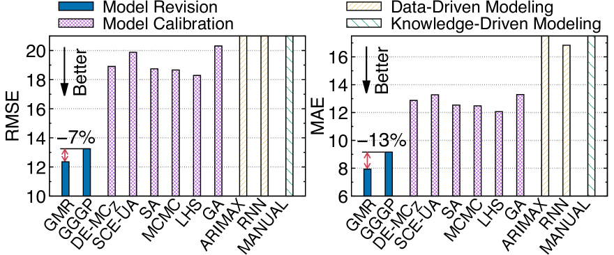
Figure 1: GMR achieves the best forecasting accuracy in the river modeling task, obtaining 7% and 13% lower RMSE (left) and MAE (right), respectively, than the second best method, while producing revised models guided by domain knowledge.

The rest of the paper is organized as follows. We describe the river modeling problem in Section II, and present the GMR framework and how to apply it to river modeling in Section III. After presenting experimental results in Section IV, we review related works in Section V, and conclude in Section VI.

II River Water Quality Modeling

Rivers are precious freshwater resources for households, farming, and industry. Due to intensive use and increasing development, the eutrophication (over-enrichment with nutrients) of rivers has become a serious global problem. Algal blooms are one of the most problematic and widespread consequences that deteriorate river water quality [19]. For improved river management, it is crucial to have an accurate model of the water quality.

River water quality modeling aims to predict phytoplankton biomass, a proxy for eutrophication. Based on the knowledge of a freshwater ecologist, we designed the following biological processes, modeling the change of phytoplankton biomass over time by capturing the interplay between phytoplankton ($B_{Phy}$) and zooplankton ($B_{Zoo}$).

$$\frac{d{B_{\mathit{Phy}}}}{dt} =B_{\mathit{Phy}}\cdot({\mu}_{\mathit{Phy}}-{\gamma}_{\mathit{Phy}})-B_{\mathit{Zoo}}\cdot\varphi$$ (1)

$$\mu_{\mathit{Phy}} =C_{\mathit{UA}}\cdot f(V_{\mathit{lgt}})\cdot g(V_{n},V_{p},V_{si})\cdot h(V_{\mathit{tmp}})$$

$$\gamma_{\mathit{Phy}} =C_{\mathit{BRA}}$$

$$\varphi =C_{\mathit{MFR}}\cdot\mathit{\lambda_{Phy}}$$

$$\mathit{\lambda_{Phy}} =({B_{\mathit{Phy}}}-C_{\mathit{Fmin}})/(C_{\mathit{FS}}+B_{\mathit{Phy}}-C_{\mathit{Fmin}})$$

$$f(V_{\mathit{lgt}}) =(V_{\mathit{lgt}}/C_{\mathit{BL}})\cdot e^{1-(V_{\mathit{lgt}}/C_{\mathit{BL}})}$$

$$g(V_{n},V_{p},V_{\mathit{si}}) =\min\left(V_{n}/(C_{N}+V_{n}),V_{p}/(C_{P}+V_{p}),V_{si}/(C_{SI}+V_{si})\right)$$

$$h(\mathit{V_{tmp}}) =\max(e^{-C_{\mathit{PT}}(V_{\mathit{tmp}}-C_{\mathit{BTP1}})^{2}},e^{-C_{\mathit{PT}}(V_{\mathit{tmp}}-C_{\mathit{BTP2}})^{2}})$$

$$\small\frac{d{B_{\mathit{Zoo}}}}{dt} ={B_{\mathit{Zoo}}}\cdot({\mu}_{\mathit{Zoo}}-{\gamma}_{\mathit{Zoo}}-{\delta}_{\mathit{Zoo}})$$ (2)

$${\mu}_{\mathit{Zoo}} =C_{\mathit{UZ}}\cdot\mathit{\lambda_{Phy}}$$

$${\gamma}_{\mathit{Zoo}} =C_{\mathit{BRZ}}+C_{\mathit{BMT}}\cdot\varphi$$

$${\delta}_{\mathit{Zoo}} =C_{\mathit{DZ}}$$

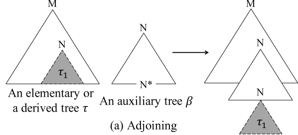
Figure 2: Illustrations of tree composition operations used by tree-adjoining grammar (TAG): (a) adjoining and (b) substitution.

The phytoplankton dynamics model (${d{B_{\mathit{Phy}}}}/{dt}$) incorporates the photosynthetic productivity (${\mu}_{\mathit{Phy}}$), metabolic degradation (${\gamma}_{\mathit{Phy}}$), and grazing pressure of zooplankton ($\varphi$). The photosynthetic productivity depends on multiplicative influences from variables such as light intensity ($V_{lgt}$), nutrient (nitrogen, phosphorus, and silica) concentrations ($V_{n},V_{p},V_{si}$), and water temperature ($V_{tmp}$). These functions build on earlier studies on modeling algal dynamics including [20, 21]. Further, considering the effect of summer cyanobacteria and winter diatom blooms, we extend the process with two additional parameters reflecting optimal temperatures ($C_{BTP1},C_{BTP2}$). The zooplankton dynamics model (${d{B_{\mathit{Zoo}}}}/{dt}$), adapted from [21], incorporates the growth (${\mu}_{Zoo}$), respiration (${\gamma}_{Zoo}$), and death (${\delta}_{Zoo}$) rates of zooplankton.

The parameters of these biological processes fall into two classes: constant parameters (starting with $C$) have constant values representing physiological rates (e.g., growth or feeding rate), while variable parameters (starting with $V$) correspond to external conditions and forces, changing over time. In evaluating (1) and (2), variable parameters are imported from the observed data at the evaluation time $t$. More details on these constant and variable parameters are given in Tables IV and III.

The goal of model revision for our task is summarised as:

River modeling is a challenging task. Although carefully built with domain knowledge, manually-designed processes (1) and (2) (Manual) exhibit poor predictive performance, as shown in Figure 1. While the results of model calibration methods show that parameter tuning greatly improves modeling accuracy, it is not enough to be able to update only the model parameters. By improving the process itself via model revision, our method obtains the best result, with 13% and 34% smaller MAE than is obtained with the second best method and the best model calibration result, respectively, while producing revised processes guided by prior knowledge.

III Methods

In this section, we present our genetic model revision (GMR) framework. There are three major challenges in applying model revision to the modeling of dynamical systems.

1. Representation of dynamic processes. Given differential equations that model dynamic processes, such as the one underlying river water quality ((1) and (2)), how can we represent them for successful model revision?

2. Mechanism for knowledge-guided model revision. Model revision requires defining specific steps for making revisions to obtain a better model. How can we effectively perform model revision guided by prior knowledge?

3. Efficient and effective model revision. Real-world systems are complex, often incurring high computational cost. How can we perform efficient and effective model revision?

In the GMR framework, we address these challenges with the following ideas.

1. Using tree-adjoining grammar (TAG) for representing dynamic processes provides a powerful framework to succinctly express dynamic processes and their revision, while facilitating controlled incorporation of prior knowledge.

2. Making revision via TAG-guided GP and expressing prior knowledge using the TAG formalism leads to an accurate model consistent with prior knowledge.

3. Removing redundancy, speeding up operations, and local search enable fast and effective model revision.

We describe how to represent dynamic processes using TAG in Section III-A, and present the GMR framework in Section III-B. Then we demonstrate how to apply GMR to real-world problems, such as river modeling, in Section III-C, and present techniques to improve efficiency and effectiveness in Section III-D.

III-A Representing Dynamic Processes Using TAG

III-A1 Preliminaries on TAG (Tree-Adjoining Grammar)

A TAG is a tree generating system [22], consisting of a quintuple ($T$, $N$, $I$, $A$, $S$) where

• $T$ is a finite set of terminal symbols;

• $N$ is a finite set of non-terminal symbols ($N\cap T=\emptyset$);

• $S\in N$ is a non-terminal symbol called the start symbol;

• $I$ is a set of finite trees called initial trees or $\alpha$-trees;

• $A$ is a set of finite trees called auxiliary trees or $\beta$-trees.

Figures 3 and 2 provide illustrations of $\alpha$- and $\beta$-trees. The trees in $I\cup A$ (i.e., $\alpha$- and $\beta$-trees) are referred to as elementary trees. In an elementary tree, the labels of all interior nodes are non-terminal symbols, while the labels of the nodes on the frontier can be either terminal or non-terminal symbols. The frontier nodes of an elementary tree with non-terminal symbols are marked as $\downarrow$ for substitution, except for one special node in an auxiliary tree, which is called the foot node and marked with an asterisk ($*$) by convention. The foot node must have the same non-terminal symbol as that of the corresponding tree’s root node (e.g., see Figure 3(b)).

Adjoining and substitution are the two composition operations TAG uses to construct a derived tree (Figure 2). Adjoining builds a new tree given an auxiliary tree $\beta$ and a tree $\tau$ (which can be either an elementary or a derived tree). Assume that the root of $\beta$ is labeled as $N$, and that the tree $\tau$ has an interior node $n$ labeled as $N$. The steps for adjoining $\beta$ into $\tau$ are as follows (see Figure 2(a) for an illustration):

1. The sub-tree $\tau_{1}$ rooted at node $n$ is disconnected from $\tau$;

2. The tree $\beta$ is attached at the place where the node $n$ was;

3. $\tau_{1}$ is attached to the foot node (marked with $*$) of the tree $\beta$.

Substitution creates a derived tree from an elementary tree $\tau$ and a tree $\alpha$ which is (derived from) an initial tree. As in Figure 2(b), substitution selects a non-terminal on the frontier of the tree $\tau$ (marked as $\downarrow$) matching the root of $\alpha$, and replaces it with $\alpha$. A tree derived from an initial tree, and lacking frontier non-terminals, is a completed tree.

An in-depth description of TAG appears in [22, 16].

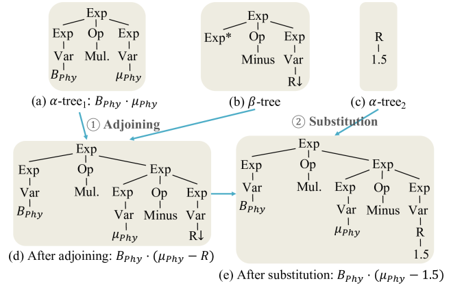
Figure 3: (a)–(c): Example $\alpha$- and $\beta$- trees representing a dynamic process and potential revisions. (d), (e): Resulting trees after adjoining and substitution (see text for details).

Figure 4: TAG derivation tree which encodes a revised differential equation. Two nodes (labeled by $\beta 1$ and $\beta 2$) are $\beta$-trees that are adjoined into the specified address (the number on the link) of the root. Rectangles contain $\alpha$-trees (lexemes), which are substituted into the open nodes in the linked tree.

III-A2 TAG-Based Dynamic Process Representation

Consider this equation, a simplified form of (1), to see how TAG can represent dynamic processes and potential revisions:

$$\frac{d{B_{\mathit{Phy}}}}{dt} =B_{\mathit{Phy}}\cdot{\mu}_{\mathit{Phy}}$$ (3)

(3) can be represented by an $\alpha$-tree shown in Figure 3(a) where “Mul.” denotes multiplication. Figure 3(b) shows a $\beta$-tree representing one potential extension where an expression (denoted by “Exp”) is extended by deducting a random variable (denoted by “R”) from it. Then adjoining the $\beta$-tree in Figure 3(b) into the rightmost “Exp” node of the $\alpha$-tree in Figure 3(a) yields the tree shown in Figure 3(d), which corresponds to $B_{\mathit{Phy}}\cdot({\mu}_{\mathit{Phy}}-R)$. Another $\alpha$-tree in Figure 3(c) encodes a potential value for variable R. By substituting it into the frontier node R (marked with $\downarrow$) shown in Figure 3(d), we obtain a revised process:

$$\frac{d{B_{\mathit{Phy}}}}{dt} =B_{\mathit{Phy}}\cdot({\mu}_{\mathit{Phy}}-1.5).$$ (4)

A completed tree (e.g., Figure 3(e)) corresponds to a revised process. The history of adjunctions and substitutions is encoded as an object tree called the derivation tree. In other words, we encode successive model revisions and the revised process as a derivation tree in TAG. Among several proposed definitions of TAG derivation tree, we use the formulation with restricted substitution [16]:

1. The root node is labeled with an $\alpha$-tree (i.e., input process) whose root node is labeled by the start symbol $S$.

2. All other nodes are labeled with $\beta$-trees (adjunction nodes). An adjunction node is associated with an address of the node at which the adjunction took place.

3. An $\alpha$-tree that is substituted is restricted to have no children, which allows us to regard substitution as an in-node operation, and also simplifies the derivation tree greatly.

With this definition, the TAG derivation tree in GMR (Figure 4) is a tree of objects where links between objects indicate adjunction at the specified address, and each node has a list of $\alpha$-trees (called lexemes) to be substituted into the open nodes (called lexicons) in the elementary tree labeled by the node.

Note that while the above discussion describes how TAG provides a mechanism for representing and revising dynamic processes, we need a more careful design of $\alpha$- and $\beta$-trees than is shown in Figure 3, to be able to make controlled changes. For example, in order to reflect prior knowledge, we may want to adjoin the $\beta$-tree in Figure 3(b) into only one of the Exp nodes in Figure 3(a). However, with the $\beta$-tree in Figure 3(b), adjoining can happen at any of them.

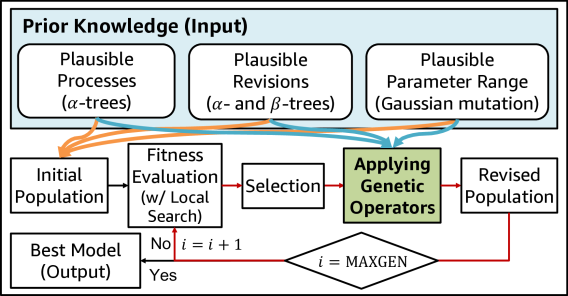
Figure 5: An overview of the model revision framework. Red loop denotes one generation. Prior knowledge shown in rounded boxes guides the entire model revision process.

III-B Knowledge-Guided Genetic Model Revision

In this section, we describe how genetic model revision is performed in our framework, and discuss how we incorporate the prior domain knowledge on (1) plausible processes, (2) plausible revisions, and (3) the model parameters.

(a) Before
crossover

(b) After
crossover

(c) Before subtree mutation

(d) After subtree mutation

(e) Before point insertion

(f) After point insertion

(g) Before point deletion

(h) After point deletion

Figure 6: An illustration of genetic operators in TAG3P.

III-B1 Framework Overview

Figure 5 shows an overview of the genetic model revision (GMR) framework. It builds upon the tree-adjoining grammar guided genetic programming (TAG3P) [23]. TAG3P is a population-based optimization algorithm that evolves a population of random (often unfit) initial programs (which are differential equations in our setting) into fitter ones for a given task, over multiple generations. TAG3P differs from standard GP in that it is a grammar-guided GP system where search space exploration is guided by TAG. In Figure 5, the loop marked in red corresponds to one generation. At each generation, genetic model revision is performed on the current population by applying genetic operators to produce a revised population of potentially fitter individuals. Note that three types of prior knowledge (shown in rounded boxes) given to the framework govern the entire search process, from population initialization to iterative model revision, until a final model is obtained.

III-B2 Framework Components

Here we detail components of our TAG3P-based framework. A detailed review of the TAG3P system can be found in [23, 16].

Representation for a program (called an individual). In our setting, a program denotes differential equations that are to be revised (e.g., biological process in (1) and (2)). In TAG3P, each program is represented as a derivation tree (Figure 4).

$\alpha$- and $\beta$-trees. In GMR, one $\alpha$-tree is used to encode manually-designed minimal process as in Figure 3(a), while other $\alpha$-trees define model revision via substitution as in Figure 3(c). $\beta$-trees are defined to represent potential revisions as in Figure 3(b). We provide more discussion on how to design these trees in Section III-B3.

Parameters. Parameters include population size (popsize), maximum number of generations (maxgen), minimum size (minsize) and maximum size (maxsize) of individuals, and the probability of genetic operators.

Population Initialization. Individuals are created repeatedly until the population size reaches popsize: TAG3P selects an individual size between minsize and maxsize, chooses an initial derivation tree randomly from $\alpha$-trees, picks up $\beta$-trees and their adjoining addresses at random, and performs adjoining to generate an individual for the first generation.

Fitness Evaluation. An individual (a derivation tree) is transformed into a derived tree, and evaluated as in standard GP. In dynamic systems modeling, this involves evaluating revised differential equations (e.g., Figure 3(e)) for each time step, and comparing it with observed values. More accurate individuals are given higher fitness.

Genetic Operators. Genetic operators make revisions to the current population to obtain others. Among several operators in TAG3P, we introduce two representative ones (Figure 6 illustrates these operations).

1. Crossover. Two individuals are chosen by a selection mechanism, and their subtrees are randomly selected and checked whether they are compatible. Subtrees are compatible if each subtree can be adjoined into the node where the other subtree is attached to. If so, the two subtrees are swapped. Otherwise, the previous process is retried unless the retry count has reached some predefined limit.

2. Subtree Mutation. A subtree $x$ is randomly selected, and is replaced with a new subtree, which is of similar size to $x$, and compatible with $x$ (to produce a valid individual).

III-B3 Incorporating Prior Knowledge

By exploring the search space of both the structure and parameters of dynamic processes, complex real-world systems can be modeled more accurately than can be achieved with parameter optimization alone. However, the resulting process might be physically implausible and violate domain knowledge. Our framework learns an accurate model that complies with prior knowledge by incorporating three types of prior knowledge.

Prior Knowledge of Plausible Processes. In an effort to explain real-world phenomena, experts develop models based on domain knowledge and experience. We harness this prior knowledge of dynamic processes, specifically what variables are known to be involved and how they interact with each other. For example, the temporal dynamics of phytoplankton $(dB_{Phy}/dt)$ in (1) is expressed as a function of zooplankton biomass $(B_{Zoo})$ (and other related parameters) since zooplankton grazing pressure is known to be a major regulator of phytoplankton in a river ecosystem. In our framework, this first type of knowledge, expressed as a differential equation, is encoded as an $\alpha$-tree as shown in Figure 3(a). Note that these input processes act as a significant knowledge transfer at the starting point of model revision. With classic GP systems, by contrast, we need to start from random models.

Prior Knowledge of Plausible Revisions. Real-world dynamic systems are complex, often consisting of multiple intertwined processes (e.g., $dB_{Phy}/dt$ and $dB_{Zoo}/dt$), each of which can be further decomposed into multiple subprocesses in a nested manner (e.g., $\mu_{Phy}$ in (1), which represents photosynthetic growth). Domain experts often have an understanding of these subprocesses, such as the functionality of the subprocess, and plausible variables that may play a role for the subprocess. For instance, variables that are known to affect photosynthetic growth include water alkalinity and the amount of dissolved oxygen. Note that this subprocess corresponds to a subtree in the $\alpha$-tree representing the input process.

Our framework allows specifying variables and operations applicable for revising a specific subprocess. This type of constraint is expressed in both $\alpha$- and $\beta$-trees. In an $\alpha$-tree, extensible subtrees are placed under a special node, whose name starts with “Ext”, denoting a revision that can be made to the corresponding subtree via tree-adjoining. In an equation form, we denote a subprocess $f(\cdot)$ extensible via “Ext” by $\{f(\cdot)\}\!\odot\!\text{Ext}$. We then generate a list of $\beta$-trees for each combination of variables and operators, which have the corresponding “Ext” as the root node, and a foot node of the same type to define allowable operations for the given subtree.

Importantly, we distinguish between the operators that are applied directly to the initial process (called connectors), and those that are applied to the subprocesses, which extend the initial process, but do not belong to the initial process (called extenders). This is to preserve the initial process by applying a limited set of operations to it, while giving a greater freedom for extenders to make improvements to the initial process.

As an example, consider again this simplified process $d{B_{\mathit{Phy}}}/dt=\{B_{\mathit{Phy}}\cdot{\mu}_{\mathit{Phy}}\}\odot\text{Ext}$, extensible via Ext. This can be encoded as an $\alpha$-tree in Figure 7(a). Note that Ext_c (denoting connectors) is used for the root node. We assume that we have two variables $B_{Zoo}$ and $R$, deduction (Minus) as a connector and multiplication (Mul.) as an extender. Figure 7(b) and (c) show two $\beta$-trees that can be generated (Ext_c and Ext_E denoting a connector and an extender). Adjoining Figure 7(a) and (b) produces $B_{\mathit{Phy}}\cdot{\mu}_{\mathit{Phy}}-B_{\mathit{Zoo}}$ in Figure 7(e); subsequently adjoining Figure 7(c) and substituting Figure 7(d) into Figure 7(e) yields a revised process $B_{\mathit{Phy}}\cdot{\mu}_{\mathit{Phy}}-B_{\mathit{Zoo}}\cdot 1.5$ in Figure 7(f) (extensions removed for brevity). Note that since connectors and extenders use different symbols (Ext_c and Ext_e), connector $\beta$-trees cannot adjoin into $\alpha$-tree nodes with extender symbols, and vice versa.

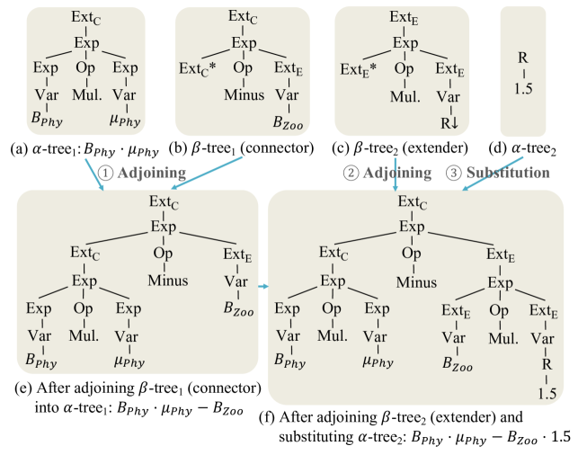
Figure 7: (a)–(d): $\alpha$- and $\beta$-trees for (a) the initial process, revision via adjoining with (b) a connector and (c) an extender, and (d) substitution. (e), (f): Resulting trees after revision via a connector and an extender (see text for details).

Prior Knowledge about Model Parameters. From previous research and experience on dynamical systems, domain experts often have the information on the plausible distributions of the model parameters. Even if we obtain a highly accurate model, if its parameters are not within a realistic range, that model is not considered a good representation of underlying processes. In GMR, the domain knowledge of model parameters is summarized as the expected value and allowed range of parameter values. For effective search, ranges need to be chosen to cover most practically feasible values. We assume that naturally occurring values follow a truncated Gaussian distribution centered around the expected value.

To optimize model parameters, we apply a genetic operator, Gaussian mutation, which locates all constant parameters in an individual, and updates them to new values sampled from their associated Gaussian distribution. In the beginning, parameters are set to the expected value. When Gaussian mutation is applied to a parameter, a new value is generated, and it becomes the new mean of the Gaussian distribution for that parameter. If the sampled value lies outside of the given range, the boundary value is used instead.

For river water quality modeling, we initially set the standard deviation to $1/4$ of the parameter mean, as that covers the range of most observable parameter values. We then ramp down the standard deviation linearly in the final $k$ generations so that it becomes smaller in later generations.

III-C Applying GMR to Real-World Problems

TABLE II: Variables, connectors, and extenders used by extensions. $R$ denotes a random variable between 0 and 1.

Extension	Variables	Extension	Variables	Extension	Variables
Ext1	$~{}V_{cd},V_{ph},V_{alk},R~{}$	Ext5	$~{}V_{tmp},R~{}$	Ext8	$~{}V_{tmp},R$
Ext2	$~{}V_{sd},R~{}$	Ext6	$~{}V_{tmp},R~{}$	Ext9	$~{}V_{tmp},R$
Ext3	$~{}V_{do},V_{ph},V_{alk},R~{}$	Ext7	$~{}V_{tmp},R~{}$
Connectors	$+$ for extensions 1–3, $\times$ for extensions 5–9
Extenders	$+,-,\times,\div,\log,\exp$ for all extensions

River Water Quality Modeling. We show how the proposed framework can be applied to the modeling of river water quality introduced in Section II, in which the goal is to make an accurate temporal prediction of the phytoplankton biomass $(B_{Phy})$. We capture the expert knowledge on the dynamics of phytoplankton ($dB_{Phy}/dt$) and zooplankton ($dB_{Zoo}/dt$), and plausible revisions as follows.

$$\frac{d{B_{\mathit{Phy}}}}{dt} =\left\{B_{\mathit{Phy}}\cdot({\mu}_{\mathit{Phy}}-{\gamma}_{\mathit{Phy}})-B_{\mathit{Zoo}}\cdot\varphi\right\}\!\odot\!\text{Ext1}$$ (5)

$$\mu_{\mathit{Phy}} =\left\{C_{\mathit{UA}}\cdot f(V_{\mathit{lgt}})\cdot g(V_{n},V_{p},V_{si})\cdot h(V_{\mathit{tmp}})\right\}\!\odot\!\text{Ext3}$$

$$\gamma_{\mathit{Phy}} =\left\{C_{\mathit{BRA}}\right\}\!\odot\!\text{Ext5}$$

$$\varphi =\left\{C_{\mathit{MFR}}\cdot\mathit{\lambda_{Phy}}\right\}\!\odot\!\text{Ext6}$$

$$\mathit{\lambda_{Phy}} =({B_{\mathit{Phy}}}-C_{\mathit{Fmin}})/(C_{\mathit{FS}}+B_{\mathit{Phy}}-C_{\mathit{Fmin}})$$

$$f(V_{\mathit{lgt}}) =(V_{\mathit{lgt}}/C_{\mathit{BL}})\cdot e^{1-(V_{\mathit{lgt}}/C_{\mathit{BL}})}$$

$$g(V_{n},V_{p},V_{\mathit{si}}) =\min\left(V_{n}/(C_{N}+V_{n}),V_{p}/(C_{P}+V_{p}),V_{si}/(C_{SI}+V_{si})\right)$$

$$h(\mathit{V_{tmp}}) =\max(e^{-C_{\mathit{PT}}(V_{\mathit{tmp}}-C_{\mathit{BTP1}})^{2}},e^{-C_{\mathit{PT}}(V_{\mathit{tmp}}-C_{\mathit{BTP2}})^{2}})$$

$$\frac{d{B_{\mathit{Zoo}}}}{dt} =\left\{{B_{\mathit{Zoo}}}\cdot({\mu}_{\mathit{Zoo}}-{\gamma}_{\mathit{Zoo}}-{\delta}_{\mathit{Zoo}})\right\}\!\odot\!\text{Ext2}$$ (6)

$${\mu}_{\mathit{Zoo}} =\left\{C_{\mathit{UZ}}\cdot\mathit{\lambda_{Phy}}\right\}\!\odot\!\text{Ext7}$$

$${\gamma}_{\mathit{Zoo}} =\left\{C_{\mathit{BRZ}}\right\}\!\odot\!\text{Ext8}+C_{\mathit{BMT}}\cdot\varphi$$

$${\delta}_{\mathit{Zoo}} =\left\{C_{\mathit{DZ}}\right\}\!\odot\!\text{Ext9}$$

Table II presents the list of variables, connectors, and extenders applicable to each extension. $R$ denotes a variable that is randomly initialized. Constant parameters (those starting with $C$) are initialized and updated via Gaussian mutation, based on their mean and exploration range given in Table III.

These extensions are defined based on an extensive river modeling experience of a freshwater ecologist, denoting different types of extensions plausible for specific subprocesses. For example, electric conductivity ($V_{cd}$) applies to the dynamics of phytoplankton via Ext1, but not to that of zooplankton.

Revising Multiple Processes. While input processes are to be represented using one $\alpha$-tree, here we have two differential equations (5) and (6). Multiple equations can be encoded as a single $\alpha$-tree by first representing each equation in separate trees, and then combining them into one $\alpha$-tree under a new, common root node. Then this combined $\alpha$-tree can be evolved in the same manner as in simpler cases, and decomposed into multiple equations when performing fitness evaluation.

Application to Other Problems. GMR provides general mechanisms to represent and revise process equations guided by prior knowledge, so is readily applicable to diverse problem settings. The only problem-dependent component is representing domain-specific knowledge as discussed in Section III-B3; this itself is a general technique applicable to various problems.

TABLE III: Constant parameters that are updated via Gaussian mutation. Prior knowledge is captured as the mean and exploration bounds (minimum and maximum values).

Description Mean Min Max Unit $\mathit{C_{UA}}$ Max growth rate of phytoplankton 1.89 0.1 4.0 day^-1 $\mathit{C_{UZ}}$ Max growth rate of zooplankton 0.15 0.0 0.3 day^-1 $\mathit{C_{BRA}}$ Breath rate of phytoplankton 0.021 0.0 0.17 day^-1 $\mathit{C_{BRZ}}$ Breath rate of zooplankton 0.05 0.0 0.2 day^-1 $\mathit{C_{MFR}}$ Maximum feeding rate 0.19 0.01 0.8 day^-1 $\mathit{C_{DZ}}$ Death rate of zooplankton 0.04 0.01 0.1 day^-1 $\mathit{C_{FS}}$ Half-saturation constant of food 5.0 4.0 6.0 $\upmu$g L^-1 $\mathit{C_{BTP1}}$ Blue-green optimal temperature 27.0 20.0 34.0 ^∘C $\mathit{C_{BTP2}}$ Diatom optimal temperature 5.0 1.0 20 ^∘C $\mathit{C_{Fmin}}$ Minimum food concentration 1.0 0.1 1.9 $\upmu$g L^-1 $\mathit{C_{BL}}$ Best light for phytoplankton 26.78 24.0 30.0 MJ m^-2 d^-1 $\mathit{C_{N}}$ Half-saturation constant of nitrogen 0.0351 0.02 0.05 mg L^-1 $\mathit{C_{P}}$ Half-saturation constant of phosphorus 0.00167 0.001 0.02 mg L^-1 $\mathit{C_{SI}}$ Half-saturation constant of silica 0.00467 0.001 0.2 mg L^-1 $\mathit{C_{BMT}}$ Breath multiplier on grazing 0.04 0.01 0.07 N/A $\mathit{C_{PT}}$ Temperature coefficient for phytoplankton growth 0.005 0.003 0.2 ^∘C^-2 $\varphi$ Grazing rate of zooplankton N/A N/A N/A d^-1

TABLE IV: Temporal variable parameters in the river process.

Parameter Description Parameter Description $V_{lgt}$ Irradiance (light intensity) $V_{do}$ Dissolved oxygen $V_{n}$ Nitrogen concentration $V_{cd}$ Electric conductivity $V_{p}$ Phosphorus concentration $V_{ph}$ pH $V_{si}$ Silica concentration $V_{alk}$ Alkalinity $V_{tmp}$ Water temperature $V_{sd}$ Water transparency

III-D Improving the Efficiency and Effectiveness

For efficient and effective optimization, we apply three orthogonal speedup techniques, together with local search.

Evaluation Short-Circuiting. Modeling temporal processes involves incremental fitness evaluation over a period of time, in which case intermediate fitness may provide a reasonable estimate of the final fitness. Also, GP is known to be robust to noisy evaluation. Based on these observations, fitness evaluation can be short-circuited, using the estimate as a surrogate of the final fitness. Early termination is such an approach where fitness evaluation is stopped when the intermediate fitness gets worse than the previous best fitness obtained from full evaluations. In GMR, we design a generalized evaluation short-circuiting technique (Algorithm 1), which allows controlling the eagerness of early termination (via the threshold parameter) and use of different extrapolation methods.

Runtime Compilation. A tree representing temporal processes needs to be evaluated multiple times over some time period, and each such evaluation can be done by recursively evaluating subtrees, providing the model parameter values appropriately at each step. Instead, we use runtime compilation, which enables more efficient evaluation than repeated tree parsing: a program encoded in the tree is converted into the corresponding source code, compiled at runtime, and dynamically loaded to be used for fitness evaluation.

Tree Caching. We cache the results of tree evaluation, and reuse them when we need to reevaluate the same trees. By using additional memory to store evaluation results, we avoid redundant computations. Note that the effectiveness of caching depends on the hit rate. GMR improves the hit rate by algebraically simplifying the trees before they are evaluated. We show the benefits of speedup techniques in Section IV-F.

Local Search. Local search aims to improve the search effectiveness by making incremental, local revisions to an individual. We apply two local search operators, insertion and deletion. Insertion randomly chooses an open adjoining address of a TAG derivation tree, and adds a randomly selected compatible auxiliary tree to the chosen location. Deletion removes a random node from the derivation tree. Figure 6 illustrates these operations. Specifically, we perform stochastic hill-climbing local search, where a tree resulting from crossover and mutation goes through a series of local search, applying insertion and deletion with equal probability, and adopting the change if it improves the fitness.

Input: ind (an individual to be evaluated), threshold (a non-negative value that determines when to check for evaluation short-circuiting), numFitcases (number of fitness cases), Extrapolate (a function to extrapolate intermediate fitness).

Output: fitness (evaluated fitness of the given individual ind).

1

2 Function FitnessEvaluation(ind, threshold, numFitcases):

3       $\textit{bestPrevFull}\leftarrow\infty$

4       $\textit{fitness}\leftarrow 0$

5       $\textit{i}\leftarrow 0$

6       while $\textit{i}<\textit{numFitcases}$ do

7             Update fitness of ind using fitness case $i$

8             if $\textit{fitness}>\textit{bestPrevFull}\times\textit{threshold}$ then

9                   estFitness $\leftarrow$ Extrapolate(fitness, i, numFitcases)

10                  if $\textit{estFitness}>\textit{bestPrevFull}$ then

                         return estFitness

                          $\triangleright$ Short Circuiting

11                        

12                  

13            $\textit{i}\leftarrow\textit{i}+1$

14      if $\textit{fitness}<\textit{bestPrevFull}$ then

15             $\textit{bestPrevFull}\leftarrow\textit{fitness}$

      return fitness

        $\triangleright$ Full Evaluation

16      

Algorithm 1 Evaluation Short-Circuiting

IV Experiments

In this section, we evaluate our GMR framework via a case study on river modeling. We address the following questions.

1. Prediction Accuracy: How accurately does the GMR framework forecast river water quality?

2. Ecological Analysis: How does GMR revise the input process, and does the revision make sense from an ecological standpoint? Which variables are important in the revision?

3. Speedup Techniques: How much do the speedup techniques improve efficiency?

IV-A Dataset and Modeling Task Description

The Nakdong River catchment in South Korea is one of the largest water-quality monitoring networks supporting long-term ecological research. Our dataset is a collection of measurements for 13 years (1996–2008) at nine stations located in the catchment; (Figure 8): six (S1–S6) are sited on the main channel, while three (T1–T3) are on major tributaries. The dataset contains five types of variables: geographical (e.g., catchment area), hydrological (e.g., flow rate), meteorological (e.g., irradiance), physicochemical (e.g., water temperature), and biological (e.g., chlorophyll a). Most were measured daily, except for nutrient concentrations and chlorophyll a, which were measured weekly (at S1) or bi-weekly (at others). For those variables measured with a longer interval, we performed linear interpolation to obtain values between measurements. Note that these measurements provide values for the temporal variables in the river process (i.e., those starting with $V$ in (1), (2) and Table II). Table IV gives a description of the temporal variables. Given these measurements, our goal is to forecast the algal biomass at the lowest station (S1) due to its geographical importance (around ten million people live near S1). Specifically, we make knowledge-guided revisions to the biological process (1) and (2) to closely estimate observed algal biomass at S1.

In addition to the biological process, river modeling involves modeling the flow of water bodies in the river (called the hydrological process). What this hydrological process models includes how water bodies are discharged from stations, how the rainfall is absorbed into the river, etc. As our focus is on improving the biological process, we use a known hydrological process Appendix A gives details of the hydrological process, and how a river system with multiple stations is implemented.

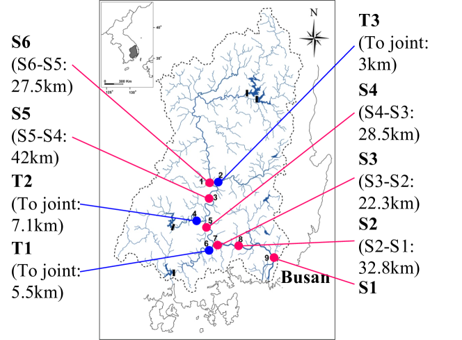
Figure 8: The Nakdong River basin in South Korea. Circles denote measuring stations. Red circles (S1–S6) are on the main channel, while blue ones (T1–T3) are on the major tributaries.

IV-B Comparators

For evaluation, we use representative comparators in the four classes of methods for modeling dynamic systems.

IV-B1 Knowledge-Driven Modeling

(a) Manual. This is the biological process in (1) and (2), designed by domain experts.

IV-B2 Data-Driven Modeling

(a) RNN (Recurrent Neural Network). We use long short-term memory (LSTM), predicting the phytoplankton biomass at S1 at the next time step from observed variables at the current time. We experiment with two variants: RNN-S1 uses variables observed at station S1 alone; RNN-All uses variables observed at all nine stations. (b) ARIMAX is widely used for time series forecasting. As with RNN, we consider two variants differing in variables used (denoted as ARIMAX-S1 and ARIMAX-All).

IV-B3 Model Calibration

Given the biological process in (1) and (2), model calibration methods optimize the values of process parameters without revising the form of equations. We use the following widely-used approaches: (a) GA (genetic algorithm) (b) MC (Monte Carlo) (c) LHS (Latin hypercube sampling) (d) MLE (maximum likelihood estimation) (e) MCMC (Markov chain Monte Carlo) (f) SA (simulated annealing) (g) DREAM (differential evolution adaptive metropolis [24]) (h) SCE-UA (shuffled complex evolution [25]) (i) DE-MC_Z (differential evolution Markov chain [26]).

IV-B4 Model Revision

(a) GGGP (grammar guided GP). We perform model revision using GGGP; that is, GGGP receives the biological process in (1) and (2) as input, and updates both the model structure and parameter values.

Appendix B provides experimental settings of all methods.

IV-C Performance Evaluation

We use RMSE (root mean square error) and MAE (mean absolute error). Let $y_{t}$ and $\hat{y}_{t}$ denote the observed and predicted values at time $t$, respectively. Given observations for $T$ time steps, we have $\mathbf{y}=(y_{1},\ldots,y_{T})$ and $\mathbf{\hat{y}}=(\hat{y}_{1},\ldots,\hat{y}_{T})$. RMSE is a quadratic score which measures the average magnitude of prediction errors, giving a relatively large weight to large errors. RMSE is defined by $\sqrt{\frac{1}{T}\!\sum_{t=1}^{T}(\hat{y}_{t}\!-\!y_{t})^{2}}$. MAE is a linear scoring rule for measuring the average magnitude of prediction errors, giving equal weights to individual differences. MAE is defined by $\frac{1}{T}\!\sum_{t=1}^{T}|\hat{y}_{t}\!-\!y_{t}|$. Both RMSE and MAE range from zero to $\infty$, and lower values indicate a better prediction.

Fitness Function. RMSE is used as a fitness function.

TABLE V: GMR achieves the best forecasting accuracy (7% and 13% more accurate than the second best method in terms of RMSE and MAE, respectively), among a variety of methods. Best results are underlined.

Method Class Method Training (96–05) Test (06–08) RMSE MAE RMSE MAE Knowledge- driven Manual 2.79e+9 2.15e+8 2.23e+6 7.93e+5 Data- driven RNN-S1 19.605 11.533 23.057 16.833 RNN-All 21.326 13.166 23.009 16.276 ARIMAX-S1 12.710 5.012   37.770 25.504 ARIMAX-All 12.365   5.775 260.468 71.471 Model calibration GA 26.329 14.693 20.308 13.291 MC 26.581 14.426 19.259 12.675 LHS 26.812 14.536 18.287 12.064 MLE 26.033 14.408 19.513 13.242 MCMC 26.514 14.554 18.661 12.480 SA 26.463 14.585 18.740 12.532 DREAM 26.825 14.853 19.281 12.581 SCE-UA 25.995 14.353 19.876 13.275 DE-MC_Z 26.227 14.432 18.904 12.869 Model revision GGGP 20.741 11.316 13.248 9.158 GMR 21.427 11.966 12.356   7.936  

IV-D Q1. Prediction Accuracy

We split the data into two periods, 1996–2005 for training and 2006–2008 for testing, and report the forecasting accuracy in Table V, in terms of the best RMSE and MAE where best models denote those with the smallest test RMSE.

Manual performed significantly worse than other approaches, although it is designed with domain knowledge of the biological process and a careful selection of parameter values. Model calibration approaches, such as GA, LHS, and SA, obtained a much better result than Manual, indicating the benefits of tuning model parameters. However, model calibration methods were outperformed by model revision methods (with GMR obtaining 32% and 34% smaller RMSE and MAE than the best model calibration results) as they can update only the model parameters, but not the model structure. In both criteria, GMR achieved the best testing performance, with 7% and 13% smaller RMSE and MAE, respectively, than the second best method GGGP.

For data driven models, we used two types of input variables. Both variants of RNN and ARIMAX (denoted by S1 and All) performed worse than model calibration and model revision methods. While RNN’s best test performance was worse than GMR, RNN could achieve much smaller training RMSE ($\scriptstyle\sim$6.7) than others as training continued. However, it suffered from overfitting and its test RMSE increased to $\scriptstyle\sim$44.0. Note that for both RNN and ARIMAX, using additional input variables observed at stations other than S1 did not help improve the performance. In fact, for predicting phytoplankton at S1, ARIMAX-All performed worse than ARIMAX-S1. As measuring stations are located over a wide area (see Figure 8), using measurements from distant stations simply as additional input features was not helpful for predicting at S1. Also, as is typically the case with ecological data, the dataset is not large enough (2,435 data points for training) for learning complex processes in a purely data-driven manner. On the other hand, by using prior knowledge, GMR can learn an effective model from a small dataset, which is also consistent with domain knowledge.

IV-E Q2. Ecological Analysis

From the perspective of ecosystem management, it is critical to understand newly added mechanisms (i.e., extensions). However, many machine learning applications to environmental research employ uninterpretable, black-box models. In this section, we strive to understand to what extent the extensions reinforce meaningful information and variables, and enhance the predictive power of the initial process model.

Case Study. We examined the best models and found that several common variables were added to specific processes. First, the addition of temperature dependence was frequently observed, particularly in zooplankton, which is an algal grazer. (7) shows an example where a revision is highlighted.

This shows that the temperature is related to the metabolic rate of zooplankton and its mortality, and plays a key role on the prediction of algal blooms.

Second, pH was often connected with algal growth process, as in the following example:

In modeling algal process in rivers, pH has not been often used in knowledge-based modeling as it is not known to be a limiting factor. Although pH is closely associated with aquatic carbon complex (which is also an essential component of photosynthesis, along with nitrogen and phosphorus), it has been neglected in modeling due to a plethora of carbon availability. However, it is remarkable to observe the improvement of predictive power when pH is considered as an input variable. In fact, recent machine learning models have illuminated pH as a crucial factor to predict algal blooms. This is one of the major discoveries by GMR in the context of river modeling, which corroborates the importance of pH in environmental research. Also, note that $V_{alk}$ is determined by $CO_{3}^{2-}$, which is in turn related to pH, and $V_{cd}$ is a reasonable selection as it is considered a proxy of pollutant concentration in freshwaters.

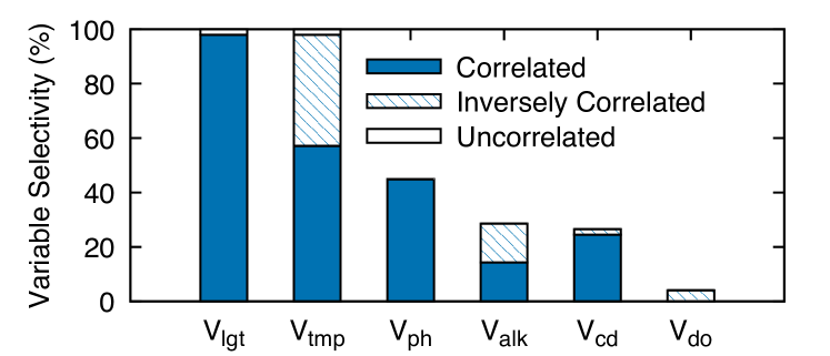
Figure 9: Selectivity of variables among the 50 best models.

Relative Importance Analysis. To assess the relative importance of input variables, we explored the selectivity (%) of variables among the 50 best models, and the correlation of each variable with phytoplankton ($B_{Phy}$) growth via variable perturbation (Figure 9). Among them, light ($V_{lgt}$) and water temperature ($V_{tmp}$) were selected most often; this agrees with the fact that they are limiting factors for phytoplankton growth. Note that while $V_{lgt}$ was consistently correlated with $B_{Phy}$, $V_{tmp}$ was not. As water temperature has multiple optimal points for the best growth of $B_{Phy}$, $V_{tmp}$ can affect $B_{Phy}$ either positively or negatively depending on the dominance of ambient phytoplankton functional group. The third important factor, $V_{ph}$, is closely related to photosynthesis and oxygen release. Alkalinity ($V_{alk}$) and electric conductivity ($V_{cd}$) were selected similarly often: $V_{cd}$’s high correlation is plausible as conductivity can be a proxy of nutrient levels in freshwater. Dissolved oxygen ($V_{do}$) was negatively correlated with $B_{Phy}$, implying that phytoplankton biomass is lower in higher $V_{do}$ concentrations. Overall, while a few exceptions exist, most selected ones were ecologically plausible and interpretable.

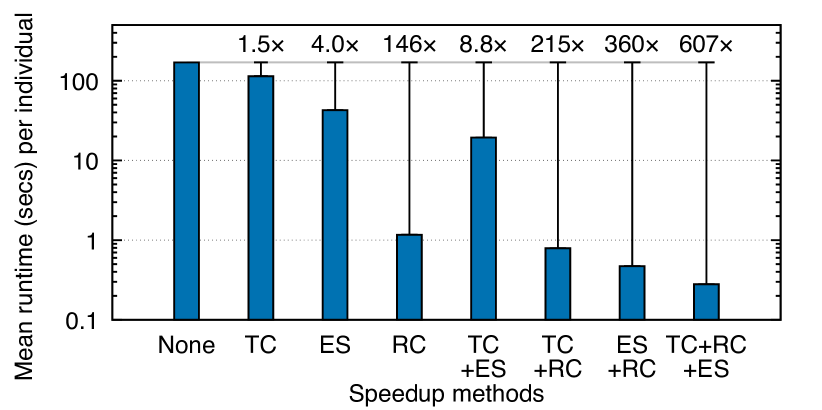
Figure 10: Mean runtime (seconds) per individual by speedup techniques. TC: Tree Caching, ES: Evaluation Short-Circuiting, RC: Runtime Compilation. Applying all leads to $607\times$ speedup.

IV-F Q3. Analysis of Speedup Techniques

We apply three orthogonal methods for speedup, i.e., tree caching (TC), evaluation short-circuiting (ES), and runtime compilation (RC). Figure 10 shows the mean runtime (seconds) per individual obtained with different speedup methods, which indicates that these techniques effectively reduce computational costs, achieving 607$\times$ speedup when all methods are applied together, compared to when no speedup techniques were used. We also measured how ES affects the performance when we use different thresholds (0.7, 1.0, and 1.3). Figure 11 shows relative values w.r.t. ES with a threshold of 1.0. Results indicate that ES generally cut down evaluation cost without sacrifice in accuracy, and nearly 100% of the best models were fully evaluated. While the overall RMSE increased by 5% as ES got eager (with a threshold of 0.7), the number of evaluated time steps dropped by 19%.

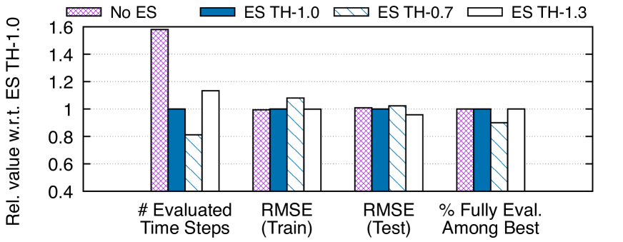
Figure 11: Effect of evaluation short-circuiting (ES) as thresholds (TH) are varied. Relative values w.r.t. ES TH-1.0 are reported.

V Related Work

Scientific Discovery from Data. Interest in computational methods for making scientific discoveries from data is growing. Among data-driven approaches, symbolic regression (SR) using GP [27] aims to discover scientific laws from data without relying on prior knowledge. While SR searches for the form of equations and their parameters simultaneously as in genetic model revision (GMR), SR may learn models that are inconsistent with domain knowledge due to the lack of guidance in the optimization process.

Combining prior knowledge and data science [9] is an emerging paradigm with promising results, which can address this challenge. One approach along this line is to guide the learning algorithm, e.g., via theory-guided constrained optimization [28, 9]. GMR also falls in this category, using TAG formalism for knowledge-guided navigation of the search space. Model calibration [9] is another such approach: data are used to optimize the parameters of a knowledge-based model. GMR outperforms various model calibration approaches, while learning knowledge-consistent processes.

Modeling River Water Quality. QUAL2E [29] is the most well-known model for river ecosystems. Despite its wide use, QUAL2E’s accuracy was limited due to their assumption on steady-state flow. Neural network (NN) and genetic algorithm (GA) have recently been used for river modeling. NN-based methods perform data-driven modeling using multilayer perceptron [30] and recurrent neural networks [31]. By performing model calibration, GA-based methods [1, 32] successfully improved the accuracy of a knowledge-based river model. However, existing evolutionary methods do not have mechanisms to jointly optimize the structure and parameters of a model, in particular, guided by domain knowledge. To fill this gap, we design novel mechanisms to represent prior knowledge and perform knowledge-guided model revision in TAG3P. As the first work on modeling river water quality using knowledge-guided model revision, our work improves upon earlier works that made limited or no use of prior knowledge.

VI Conclusion

Model revision is an effective approach for modeling real-world phenomena where domain expertise and data are used simultaneously to model complex dynamical systems. Our genetic model revision (GMR) framework performs model revision guided by prior knowledge. The case study of river modeling shows its effectiveness. In future work, we will explore new mechanisms to incorporate domain knowledge (new search operators and language biases), and apply GMR to other domains, such as financial forecasting.

Reproducibility: Code and data are available at https://www.cs.cmu.edu/~namyongp/gmr.

Extensibility: How readily can the ideas behind this work be extended to other domains? The degree of effort required depends on the similarity to the present problem. At one extreme, the underlying ideas are applicable to most model identification problems where expert knowledge is available but incomplete. TAG grammars are particularly suited to this, because they readily match the common situation where experts have a simple model that they believe to be generally correct, but potentially to require modification because potentially important processes have been omitted for simplicity. The adjunction operation of TAG3P is particularly suited to recording the way experts think about such problems. Similarly, it will frequently be the case that experts can define feasibility bounds on model parameters. In real world problems, it is frequently the case that evolving models need to be repeatedly evaluated to estimate their fitness. In such cases, the speedup techniques we have described here may well be applicable. In all these circumstances, portions of the code we have made available may be useful for implementation.

At the other extreme, the system can be directly applied to other river systems under the assumption of conservative, non-branching flow, provided that the corresponding data is available. The system also relies specifically on the G++ compiler suite to provide run-time compilation. Similar capabilities are available in other C++ compilers, or run-time compilation can be sacrificed at a substantial cost in speed.

Where the data differs in the water properties collected, revisions in the search limiting grammar will be required, and prior knowledge of the feasible values of any new parameters will need to be specified.

Extensions to river systems with substantial water loss through evaporation or leakage, or to braided streams or delta, require significant re-programming of the flow model, and additional data inputs for those components.

Moving beyond rivers, much of the structure of the system is determined by the need to model variables that change as a fluid flows through a network. It is not hard to find other problems that fit that bill: flow of blood through an organism; flow of feedstocks through a chemical plant; municipal water or sewage systems. In all these cases, the existing code would form a useful starting point.

Appendix A Further Details of River Modeling

Modeling A River System. To monitor the ecological status of a river, sample measurement is performed, often on a regular basis, at multiple measuring stations located in geographically important places. Based on this data collection scheme, we model a river system as a directed acyclic graph as shown in Figure 12, where a node corresponds to a measuring station and an edge denotes a segment of a river between the two adjacent stations. To model the confluence, we add a virtual station where two or more water bodies meet together as depicted in Figure 12 (VS₁). We model our study site shown in Figure 8 by adding six stations (S1–S6) at the main channel of the river, three stations (T1–T3) at the major tributaries of the river, and three virtual stations at the confluence of a tributary with the main stream (S6 $\cdot$ T3, S4 $\cdot$ T2, and S3 $\cdot$ T1).

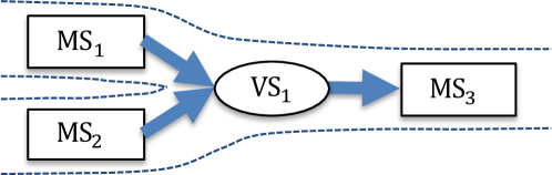
Figure 12: An example river system with measuring stations (MS) and a virtual station (VS). VS is placed at a confluence.

Hydrological Process. Modeling a river system involves modeling two contemporaneous processes, the biological and hydrological processes. The biological process shown in (1) and (2) models the evolution of phytoplankton and zooplankton and their interaction. The hydrological process models the flow of water bodies, and provides information of flow at specific time to the biological process. We use the hydrological process first introduced in [1], which is based on a flow mass balance between stations. Specifically, given that water flows from station A to station B, flow into B consists of three components, (i) inflow from upper station A, (ii) water retained at B (e.g., due to water trapped in side pools or non-laminar flow), and (iii) runoff into B from precipitation:

$$F_{B,t+\Delta}=r_{B}\cdot F_{B,t}+(1-r_{A})\cdot F_{A,t}+R_{B,t+\Delta}$$ (9)

where $F_{S,t}$ denotes the flow at station $S$ at time $t$, $r_{S}$ is the ratio of the water retained at station $S$, $\Delta$ is the time taken for water bodies from A to arrive at B, and $R_{S,t}$ denotes the amount of inflow into station B at time $t$ that arises from rain fall. Our hydrological process also models how water bodies are merged at a confluence (e.g., VS₁ in Figure 12), in which case the attributes (e.g., nutrient level) of each water body are updated based on (9) as they are moving to the confluence, and the water bodies are aggregated as a flow-weighted average.

Thus, the hydrological process determines the attributes of a water body at a specific location and time by modeling how water bodies are merged, how the rainfall is absorbed into the river, etc. As the attributes of a water body are used by the biological process, the hydrological process affects the biological process. As we focus on modeling the biological process, we use a static hydrological process in this work.

Biological Process. We evolve a population of individuals (Figure 5), where each one is a revised biological process. Each individual receives values for the temporal variables (Table IV) from the water body that the hydrological process provides, and updates the phytoplankton ($B_{Phy}$) and zooplankton ($B_{Zoo}$) according to its process equation. Tables IV and III list the variables used in our biological process.

Appendix B Experimental Settings

Environment. We used an Ubuntu server with 80 Intel Xeon E7-4850 processors at 2.00GHz and 252GB RAM.

GMR, GGGP, and GA. We implemented GMR, GGGP, and GA frameworks in C++. For GMR, we used the following configurations: number of generations (100), population size (200), number of runs (60), minimization objective (RMSE), elite size (2), number of local search steps (5), selection mechanism (tournament selection), tournament size (5), minimum chromosome size (2), maximum chromosome size (50). We applied the following genetic operators (the number in the parentheses denotes the operator probability): crossover (0.3), subtree mutation (0.3), Gaussian mutation (0.3), and replication (0.1). For GGGP and GA, we used the same configurations used for GMR. Since local search incurs additional fitness evaluation in GMR, GGGP and GA used a population of 1200 individuals to use the same number of fitness evaluation for both methods.

RNN. We used a two-layer LSTM implemented in PyTorch, whose hidden size was equal to the number of input features. The output was transformed into an estimated phytoplankton value via dense neural networks with two layers. The input features were standardized. We used Adam optimizer with $\alpha=0.01,\beta_{1}=0.9,\beta_{2}=0.999$, and weight decay of 0.0005. The model was trained for up to 1000 epochs with MSE loss.

ARIMAX. We used the pmdarima library and its Auto-ARIMA functionality with the default parameter settings.

Others. For other model calibration methods, we used the SPOTPY framework [33] using RMSE as the objective function. We set method parameters to their default values.

References

- [1] D. Kim, B. McKay, H. Shin, Y. Lee, and X. H. Nguyen, “Ecological application of evolutionary computation: Improving water quality forecasts for the nakdong river, korea,” in CEC, 2010, pp. 1–8.
- [2] C.-J. Lu, T.-S. Lee, and C.-C. Chiu, “Financial time series forecasting using independent component analysis and support vector regression,” Decision Support Systems, vol. 47, no. 2, pp. 115–125, 2009.
- [3] G. I. Webb, M. J. Pazzani, and D. Billsus, “Machine learning for user modeling,” User Model. User-Adapt. Interact., vol. 11, no. 1-2, 2001.
- [4] N. Park, E. Kang, M. Park, H. Lee, H.-G. Kang, H.-J. Yoon, and U. Kang, “Predicting acute kidney injury in cancer patients using heterogeneous and irregular data,” PLOS ONE, vol. 13, 07 2018.
- [5] N. Park, A. Kan, X. L. Dong, T. Zhao, and C. Faloutsos, “Estimating node importance in knowledge graphs using graph neural networks,” in KDD. ACM, 2019, pp. 596–606.
- [6] ——, “Multiimport: Inferring node importance in a knowledge graph from multiple input signals,” in KDD. ACM, 2020, pp. 503–512.
- [7] B. Jeon, N. Park, and S. Bang, “Dropout prediction over weeks in moocs via interpretable multi-layer representation learning,” CoRR, vol. abs/2002.01598, 2020.
- [8] O. Becker, S. Shacham, Y. Marantz, and S. Noiman, “Modeling the 3d structure of gpcrs: advances and application to drug discovery.” Current opinion in drug discovery & development, vol. 6, no. 3, 2003.
- [9] A. Karpatne, G. Atluri, J. H. Faghmous, M. S. Steinbach, A. Banerjee, A. R. Ganguly, S. Shekhar, N. F. Samatova, and V. Kumar, “Theory-guided data science: A new paradigm for scientific discovery from data,” TKDE, vol. 29, no. 10, pp. 2318–2331, 2017.
- [10] S. Džeroski, P. Langley, and L. Todorovski, “Computational discovery of scientific knowledge.” Springer, 2007, pp. 1–14.
- [11] J. R. Koza, Genetic programming - on the programming of computers by means of natural selection, ser. Complex adaptive systems. MIT Press, 1993.
- [12] R. Vyas, P. Goel, and S. S. Tambe, “Genetic programming applications in chemical sciences and engineering,” in Handbook of Genetic Programming Applications, 2015, pp. 99–140.
- [13] M. Affenzeller, S. M. Winkler, S. Wagner, and A. Beham, Genetic Algorithms and Genetic Programming - Modern Concepts and Practical Applications. CRC Press, 2009.
- [14] N. P. Dao, X. H. Nguyen, R. I. B. McKay, C. Siriteanu, Q. U. Nguyen, and N. Park, “Evolving the best known approximation to the Q function,” in GECCO, 2012, pp. 807–814.
- [15] P. A. Whigham, “Grammatical bias for evolutionary learning,” Ph.D. dissertation, New South Wales, Australia, Australia, 1996, aAI0597571.
- [16] X. H. Nguyen, “A flexible representation for genetic programming: lessons from natural language processing,” Ph.D. dissertation, University of New South Wales, Australian Defence Force Academy, 2004.
- [17] D. J. Montana, “Strongly typed genetic programming,” Evolutionary Computation, vol. 3, no. 2, pp. 199–230, 1995.
- [18] M. O’Neill and C. Ryan, “Grammatical evolution,” IEEE Transactions on Evolutionary Computation, vol. 5, no. 4, pp. 349–358, 2001.
- [19] B. R. Moss, Ecology of fresh waters: man and medium, past to future. John Wiley & Sons, 2009.
- [20] K.-J. Cho and J.-K. Shin, “Growth and nutrient kinetics of some algal species iso-lated from the naktong river,” Algae, vol. 13, no. 2, 1998.
- [21] P. Hongping and M. Jianyi, “Study on the algal dynamic model for west lake, hangzhou,” Ecological Modelling, vol. 148, no. 1, pp. 67–77, 2002.
- [22] A. K. Joshi and Y. Schabes, “Tree-adjoining grammars,” in Handbook of formal languages. Springer, 1997, pp. 69–123.
- [23] X. H. Nguyen, R. I. McKay, and H. A. Abbass, “Tree adjoining grammars, language bias, and genetic programming,” in EuroGP, 2003.
- [24] J. A. Vrugt, “Markov chain monte carlo simulation using the dream software package: Theory, concepts, and matlab implementation,” Environmental Modelling & Software, vol. 75, pp. 273–316, 2016.
- [25] Q. Duan, S. Sorooshian, and V. K. Gupta, “Optimal use of the sce-ua global optimization method for calibrating watershed models,” Journal of hydrology, vol. 158, no. 3-4, pp. 265–284, 1994.
- [26] J. A. Vrugt, C. J. Ter Braak, M. P. Clark, J. M. Hyman, and B. A. Robinson, “Treatment of input uncertainty in hydrologic modeling: Doing hydrology backward with markov chain monte carlo simulation,” Water Resources Research, vol. 44, no. 12, 2008.
- [27] M. Schmidt and H. Lipson, “Distilling free-form natural laws from experimental data,” science, vol. 324, no. 5923, pp. 81–85, 2009.
- [28] A. Karpatne, W. Watkins, J. S. Read, and V. Kumar, “Physics-guided neural networks (PGNN): an application in lake temperature modeling,” CoRR, vol. abs/1710.11431, 2017.
- [29] L. C. Brown and T. O. Barnwell, The enhanced stream water quality models QUAL2E and QUAL2E-UNCAS: Documentation and user manual. US Environmental Protection Agency. Office of Research and Development, Environmental Research Laboratory., 1987.
- [30] K. P. Singh, A. Basant, A. Malik, and G. Jain, “Artificial neural network modeling of the river water quality–a case study,” Ecological Modelling, vol. 220, no. 6, pp. 888–895, 2009.
- [31] K. Kim, D.-K. Kim, J. Noh, and M. Kim, “Stable forecasting of environmental time series via long short term memory recurrent neural network,” IEEE Access, vol. 6, pp. 75 216–75 228, 2018.
- [32] M. Kim, N. Park, R. B. McKay, H. Shin, Y.-G. Lee, K.-S. Jeong, and D.-K. Kim, “Improvement of complex and refractory ecological models: Riverine water quality modelling using evolutionary computation,” Ecological Modelling, vol. 291, pp. 205–217, 2014.
- [33] T. Houska, P. Kraft, A. Chamorro-Chavez, and L. Breuer, “Spotting model parameters using a ready-made python package,” PloS one, vol. 10, no. 12, p. e0145180, 2015.