Mitigating Edge Machine Learning Inference Bottlenecks:
An Empirical Study on Accelerating Google Edge Models

Abstract

As the need for edge computing grows, many modern consumer devices now contain edge machine learning (ML) accelerators that can compute a wide range of neural network (NN) models while still fitting within tight resource constraints. We analyze a commercial Edge TPU using 24 Google edge NN models (including CNNs, LSTMs, transducers, and RCNNs), and find that the accelerator suffers from three shortcomings, in terms of computational throughput, energy efficiency, and memory access handling. We comprehensively study the characteristics of each NN layer in all of the Google edge models, and find that these shortcomings arise from the one-size-fits-all approach of the accelerator, as there is a high amount of heterogeneity in key layer characteristics both across different models and across different layers in the same model.

We propose a new acceleration framework called Mensa. Mensa incorporates multiple heterogeneous ML edge accelerators (including both on-chip and near-data accelerators), each of which caters to the characteristics of a particular subset of models. At runtime, Mensa schedules each layer to run on the best-suited accelerator, accounting for both efficiency and inter-layer dependencies. As we analyze the Google edge NN models, we discover that all of the layers naturally group into a small number of clusters, which allows us to design an efficient implementation of Mensa for these models with only three specialized accelerators. Averaged across all 24 Google edge models, Mensa improves energy efficiency and throughput by 3.0x and 3.1x over the Edge TPU, and by 2.4x and 4.3x over Eyeriss v2, a state-of-the-art accelerator.

1 Introduction

Modern consumer devices make widespread use of machine learning (ML). The growing complexity of these devices, combined with increasing demand for privacy, connectivity, and real-time responses, has spurred significant interest in pushing ML inference computation to the edge (i.e., into these devices, instead of in the cloud) [53, 55, 6]. Due to the resource-constrained nature of edge platforms, they now employ specialized energy-efficient accelerators for on-device inference (e.g., Google Edge TPU [17], NVIDIA Jetson [41], Intel Movidius [27]). At the same time, neural network (NN) algorithms are evolving rapidly, which has led to many types of NN models (e.g., CNNs [49], LSTMs [44], GRUs [10], Transducers [24, 21], hybrid models [11, 52]), each targeting various applications (e.g., face detection [49], speech recognition [24, 38, 44], translation [54], image captioning [52, 11]).

Google’s state-of-the-art Edge TPU [17] provides an optimized one-size-fits-all solution across this wide variety of NN models, while being mindful of edge device area and energy constraints. Unfortunately, we find that it is very challenging to simultaneously achieve high energy efficiency ($\mathrm{TFLOP}\text{/}\mathrm{J}$), computational throughput ($\mathrm{TFLOP}\text{/}\mathrm{s}$), and area efficiency ($\mathrm{TFLOP}\text{/}{\mathrm{mm}}^{2}$) for each workload with this one-size-fits-all approach. We conduct an in-depth analysis of inference execution on a commercial Edge TPU, across 24 state-of-the-art Google edge models spanning four popular NN model types: (1) CNNs, (2) LSTMs [44], (3) Transducers [24, 38, 43], and (4) RCNNs [52, 11]. These models are used in several Google mobile applications, such as image classification, object detection, semantic segmentation, automatic speech recognition, and image captioning. Based on our analysis (Section 3), we find that the accelerator suffers from three major shortcomings. First, the accelerator utilizes only 1/4 of its peak throughput, averaged across all models (and less than 1% utilization for LSTMs and Transducers, the worst case). Second, despite using specialized logic, the accelerator provides only 37% of its theoretical peak energy efficiency ($\mathrm{TFLOP}\text{/}\mathrm{J}$) on average. Third, the accelerator’s memory system is often a large bottleneck. As an example, while large on-chip storage buffers (e.g., several megabytes) account for a significant portion of energy consumption (e.g., 48.1% static and 36.5% dynamic energy during CNN inference), they are often ineffective at reducing off-chip accesses, and cannot accommodate the parameters of larger NN models.

To identify the root cause of these shortcomings, we perform the first comprehensive per-layer analysis of the Google edge NN models, and make two key observations. First, there is significant variation in terms of layer type, shape, and characteristics (e.g., $\mathrm{FLOP}\mathrm{/}{Byte}$ ratio, footprint, intra- and inter-layer dependencies) across the models. For example, Transducer layers differ drastically (by as much as two orders of magnitude) from CNN layers in terms of parameter footprint and $\mathrm{FLOP}\text{/}\mathrm{B}$. Second, even within each model, there is high variation in terms of layer types and shapes (e.g., pointwise, depthwise, fully-connected, standard convolution, recurrent). This leads to up to two orders of magnitude of variation for layer characteristics within a single model. We quantify for the first time how intra-model variation is dramatically higher in edge models compared to previously-studied traditional models (e.g., [35, 49]), as edge models employ several techniques (e.g., separable convolutions [26, 25]) to reduce computational complexity and layer footprint, in order to optimize the models for resource-constrained edge devices.

Despite this large variation, many state-of-the-art edge ML accelerators [17, 27, 28, 41, 16, 14] take a monolithic design approach, where they equip the accelerator with a large PE array, large on-chip buffers, and a fixed dataflow (e.g., output stationary). While this approach might work for a specific group of layers (e.g., traditional convolutional layers with high compute intensity and high data reuse), we find that it leads to throughput and energy efficiency shortcomings across the significantly more diverse edge NN models, as illustrated by two examples. First, in the memory system, state-of-the-art accelerators employ highly overprovisioned on-chip buffers that are unable to effectively reduce off-chip parameter traffic and provide high bandwidth to PEs, leading to PE underutilization. Second, state-of-the-art accelerators use a fixed dataflow across all layers. Due to the drastic variation across different layers, the fixed dataflow often misses spatial/temporal reuse opportunities across layers.

A number of recent works [6, 37] cater to NN variation by enabling reconfigurability for parts of the accelerator. For example, Eyeriss v2 [6] provides the ability to reconfigure the on-chip interconnect and make use of a smaller PE array. Unfortunately, as models become more diverse and go beyond the structure of more traditional CNNs, reconfigurable accelerators face three issues: (1) they do not provide the ability to reconfigure a number of essential design parameters (e.g., on-chip buffers, memory bandwidth); (2) they can require frequent online reconfiguration to cater to increasing intra-model heterogeneity, with associated overheads; and (3) they make it difficult to co-design the dataflow with key components such as the memory system. The key takeaway from our extensive analysis of Google edge NN models on the Edge TPU is that all key components of an edge accelerator (i.e., PE array, dataflow, memory system) must be co-designed based on specific layer characteristics to achieve high utilization and energy efficiency. Our goal is to revisit the design of edge ML accelerators such that they are aware of and can fully exploit the growing variation within and across edge NN models.

To this end, we propose Mensa, the first general HW/SW composable framework for ML acceleration in edge devices. The key idea of Mensa is to incorporate and manage layer execution across multiple on-chip and near-data accelerators, each of which is small and tailored to the characteristics of a particular subset of layers. As we study the characteristics of different layers in our edge models, we make an important discovery: the layers naturally group into a small number of clusters that are based on a subset of these characteristics. This allows us to limit the number of different accelerators in a Mensa design to the number of clusters (five for our Google edge models). We design a runtime for Mensa to determine which of these accelerators should execute each of the layers, using information about (1) which accelerator is best suited to the layer’s characteristics, and (2) inter-layer dependencies.

Using our insight about layer clustering, we develop one possible design for Mensa that is optimized for our Google edge workloads. We find that our accelerator designs should center around two key layer characteristics (memory boundedness, and activation/parameter reuse opportunities). Of our five clusters, Clusters 1 and 2 have similar key characteristics, as do Clusters 4 and 5, allowing us to reduce the number of accelerators needed in our example implementation to three (which we call Pascal, Pavlov, and Jacquard). Pascal (for compute-centric layers) uses a dataflow that enables temporal reduction of output activations and spatial multicasting of parameters. This dataflow allows us to design a memory system with an on-chip buffer that is 16x smaller than our baseline Edge TPU, and greatly reduces on-chip network traffic, while still keeping the processing elements (PEs) highly utilized. Pavlov (for LSTM-like data-centric layers) uses a dataflow that enables temporal reduction of output activations, and identifies opportunities to schedule the parallel execution of layer operations in a way that improves parameter reuse, reducing off-chip parameter traffic. Jacquard (for other data-centric layers) uses a dataflow that exposes reuse opportunities in parameters and reduces the size of the parameter buffer. We provide both of our data-centric accelerators with high memory bandwidth by placing them in the logic layer of 3D-stacked memory, and use significantly smaller PE arrays for the accelerators compared to the PE array in Pascal.

Our evaluation shows that compared to our baseline Edge TPU, Mensa reduces total inference energy by 66.0%, improves energy efficiency ($\mathrm{TFLOP}\text{/}\mathrm{J}$) by 3.0x, and increases computational throughput ($\mathrm{TFLOP}\text{/}\mathrm{s}$) by 3.1x (averaged across all 24 Google edge NN models). Mensa improves inference energy efficiency and throughput by 2.4x and 4.3x over Eyeriss v2, a state-of-the-art accelerator.

We make the following contributions in this work:

• We conduct the first in-depth analysis of how the Google Edge TPU operates across a wide range of state-of-the-art Google edge NN models. Our analysis reveals three key shortcomings of the Edge TPU for these models: (1) poor throughput due to significant PE underutilization, (2) low energy efficiency, and (3) a large memory bottleneck.

• We comprehensively analyze the key characteristics of each layer in 24 Google edge NN models. We make three observations from our analysis: (1) layer characteristics vary significantly both across models and across layers within a single model, (2) the monolithic design of state-of-the-art accelerators (e.g., the Edge TPU) is the root cause of their shortcomings, and (3) layers naturally group into a small number of clusters based on their characteristics.

• We propose Mensa, a new framework for efficient edge ML acceleration. Mensa is the first accelerator to exploit the significant compute and memory demand heterogeneity that we observe in state-of-the-art edge NN models, through the use of a runtime scheduler and a few small, carefully specialized accelerators.

• We create a Mensa design for our Google edge models, and find that it is significantly more energy efficient and provides higher throughput than a commerical Edge TPU and Eyeriss v2, a state-of-the-art ML accelerator.

2 Background

CNNs. Convolutional neural networks (CNNs) are feed-forward models that successfully capture spatial features. A CNN is mostly composed of convolutional layers. Each convolutional layer (1) performs a 2D convolution operation between the input activations and parameters from kernels, and (2) passes the result through a non-linear activation function (e.g., ReLU, sigmoid, tanh) to produce the output activations.

LSTMs. Long short-term memories (LSTM) are a class of NNs that are effective for sequence-to-sequence application domains. An LSTM contains recurrent connections that allow the model to propagate and maintain context information across the input sequence. At each step, an LSTM makes a prediction based on the current input ($x_{t}$) and activations from the previous time step ($h_{t-1}$).

The LSTM network consists of multiple LSTM layers, where each includes several LSTM cells. Each LSTM cell has four gates (input, forget, update, and output) that allow the cell to regulate the information flow and update the cell state accordingly. At each step, the cell receives the input ($x_{t}$) and input hidden vector ($h_{t-1}$), which is the output hidden vector from the previous cell (i.e., the recurrent connection). Each gate performs two matrix-vector multiplies (MVM): (1) an input MVM with the input parameter matrix ($W_{x}$) and the input vector ($x_{t}$), and (2) a hidden MVM with the hidden parameter matrix ($W_{h}$) and the input hidden vector ($h_{t-1}$).

Transducers. Transducers are the state-of-the-art NN model for end-to-end automatic speech recognition systems [24, 21, 38, 43]. A transducer has three major blocks: (1) an encoder, which receives acoustic features and converts them into a high-level representation; (2) a prediction network, which generates linguistic outputs (i.e., high-level representation) that depend on the entire sequence of labels; and (3) a joint, which is a feed-forward joint that receives inputs from both the encoder and a prediction network that depends only on label histories. The encoder, prediction, and joint blocks are typically implemented by stacking several LSTM layers.

RCNNs. Recurrent convolutional neural networks (RCNNs; also known as LRCN [11]) are a class of hybrid NN models that attempt to capture spatio-temporal information [52, 34, 47, 56, 9]. RCNNs leverages the success of CNNs in extracting spatial features, and combine them with LSTM-based models that excel at detecting temporal relationships. RCNNs typically employ multiple convolutional layers in the front end of the network to perform feature extraction on input data, and then pass the CNN layer output to an LSTM-based model that performs sequence prediction.

3 TPU & Model Characterization

We analyze 24 Google edge models (including CNNs, LSTMs, Transducers, and RCNNs) using a commercial Edge TPU as our baseline accelerator. The Edge TPU has a generic tiled architecture, similar to other state-of-the-art accelerators [7, 15, 16, 31]. It includes a 2D array of PEs (64x64), where each PE has a small register file to hold intermediate results. The accelerator has two large SRAM-based on-chip buffers to hold model parameters and activations [18].

3.1 Google Edge TPU Shortcomings

1. The accelerator often suffers from extreme underutilization of the PEs. The Edge TPU has a theoretical peak throughput of $2\text{\,}\mathrm{TFLOP}\text{/}\mathrm{s}$, which is orders of magnitude higher than CPUs and GPUs. However, the accelerator operates much lower than peak throughput during inference execution (75.6% lower on average). Figure 1 (left) shows the roofline model of throughput for the Edge TPU, along with the measured throughput of all of our edge models. The PE utilization is consistently low across all models. Transducer and LSTM models have the most underutilization, with both achieving less than 1% of peak throughput. While CNN and RCNN models do somewhat better, they achieve only 40.7% of peak utilization on average (going as low as 10.2%).

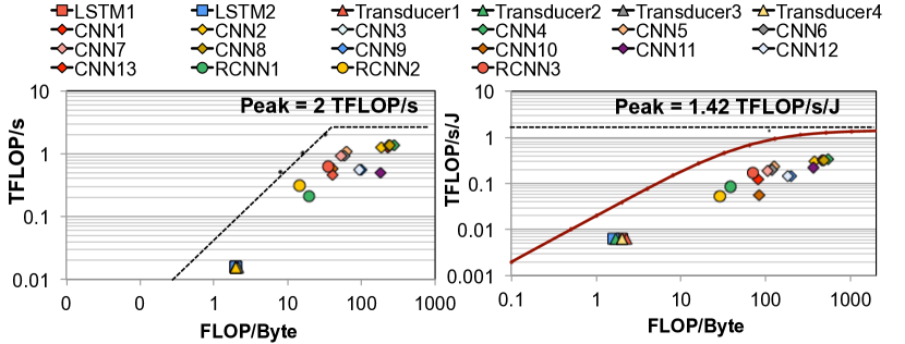
Figure 1: Throughput roofline (left) and energy roofline (right) for the Edge TPU across all models.

2. Despite using specialized logic, the Edge TPU operates far below its theoretical maximum energy efficiency. We use a similar approach to prior work [8] to obtain a roofline for energy efficiency. Figure 1 (right) shows the energy roofline for Edge TPU, along with the efficiency achieved with each model. Note that unlike the throughput roofline model, the energy roofline is a smooth curve because we cannot hide memory energy (as opposed to memory transfer time, which can be overlapped with computation time and results in the sharp knee for the throughput roofline). We find that across all models, the accelerator fails to get close to the maximum energy efficiency, falling 62.4% lower on average. The energy efficiency is particularly low (33.8% on average) for LSTM and Transducer models, but even the best CNN model achieves only 50.7% of the maximum efficiency.

3. The accelerator’s memory system design is neither effective nor efficient. Figure 2 shows the energy breakdown during inference execution across different models. We make three key observations from this figure. First, on-chip buffers account for a significant portion of both static and dynamic energy, mostly because of their large size . For example, for CNN models, 48.1% of the static energy and 36.5% of the dynamic energy is spent on accessing and storing parameters in the on-chip buffers. Second, while the buffers consume a significant amount of area (79.4% of the total accelerator area) and energy, they often do not reduce off-chip memory accesses. For Transducers and LSTMs, only 11.9% of the model parameters can fit into the buffer, and for CNNs the on-chip buffer can accommodate only 15.0% of the parameters on average. Increasing the buffer size does not help: if we increase the buffer size to 8x, this provides a latency and energy reduction of only 37.6% and 40.3%, respectively, for Transducers. This is because (1) even such a large buffer can cache only 46.5% of the parameters; and (2) the leakage and access energy increase significantly with a larger buffer size, offsetting other benefits of a larger capacity. Third, both on-chip (i.e., distributing parameters from the on-chip buffer to the PEs) and off-chip (i.e., accesses to DRAM) network traffic for model parameters results in high energy and performance costs. On average, 50.3% of the total Edge TPU energy is spent on off-chip parameter traffic (DRAM accesses and off-chip interconnect), and 30.9% of the total energy is spent on on-chip parameter traffic. We conclude that the Edge TPU’s memory system is highly inefficient.

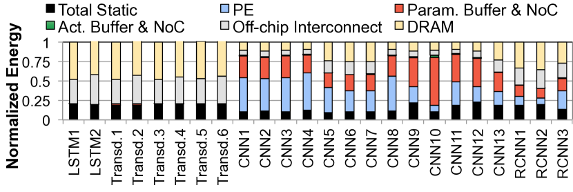
Figure 2: Energy breakdown during inference execution.

3.2 Layer-Level Study of Google Edge Models

To understand where the Edge TPU’s [17] pitfalls come from, we analyze the models themselves in significant detail.

3.2.1 Analysis of LSTMs and Transducers

We identify three key properties of LSTMs and Transducers in our edge model analysis.

1. Large parameter footprint. Each gate in an LSTM cell has an average of 2.1 million parameters, which includes parameters for both input ($W_{x}$) and hidden ($W_{h}$) matrices (as shown in Figure 3, left). The large parameter footprint of LSTM gates results in large footprints for LSTM layers (up to 70 million parameters), and in turn, LSTM and Transducer models that include such layers. Figure 3 (right) shows the total footprint vs. the $\mathrm{FLOP}\text{/}\mathrm{B}$ ratio (which indicates arithmetic intensity) across the layers of representative CNNs, LSTMs, and Transducers (the trend is the same across all models). We observe from the figure that that layers from LSTMs and Transducers have significantly larger footprints (with an average footprint of $33.4\text{\,}\mathrm{MB}\text{/}$) than layers from CNNs.

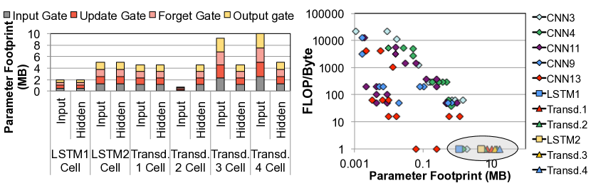
Figure 3: Parameter footprint of $W_{x}$ and $W_{h}$ for different LSTM gates for LSTMs and Transducers (left), and layer parameter footprint vs. $\mathrm{FLOP}\text{/}\mathrm{B}$ (right).

2. No data reuse and low computational complexity. For these layers, the $\mathrm{FLOP}\text{/}\mathrm{B}$ of both $W_{x}$ and $W_{h}$ is one, as shown in Figure 3 (right). The accelerator fetches $W_{x}$ and $W_{h}$ for each LSTM gate from DRAM, accesses them once to perform the input and hidden MVMs, and then does not touch the parameters again until the next LSTM cell computation, resulting in no reuse. Furthermore, these models have much a lower computational complexity than CNNs and RCNNs, with 67% fewer MAC operations on average.

3. Intra- and inter-cell dependencies. Two types of dependencies exist within LSTM layers, both of which affect how the accelerator schedules gate computations: (1) inter-cell dependencies, which are due to recurrent connections ($h_{t}$) across cells; and (2) intra-cell dependencies, which enforce the following order between gates: all four gate computation need to be done before the cell state ($c_{t}$) gets updated, after which the hidden vector ($h_{t}$)) is generated. To respect these dependencies, the accelerator schedules cells computation in a sequential manner. This means that cell computation cannot start until $h_{t-1}$ is generated by the previous cell. For each LSTM cell, the accelerator treats each gate as two fully-connected (FC) layers (corresponding to input MVM and hidden MVM), and runs the gates sequentially.

However, we find that this scheduling is not efficient. Due to the sequential execution of FC layers, the latency of updating $c_{t}$ and generating $h_{t}$ become significantly higher, which in turn degrades PE utilization (as the PEs spend more time waiting for cell calculation to be completed). We find that, despite these dependencies, there are still multiple ways to parallelize computations within LSTM cells and improve PE utilization. For example, gates within each cell can be scheduled in any order, since there are no dependencies between the gates, and the input and hidden MVMs within each gate are independent. Since the scheduler in the baseline accelerator simply treats each gate computation as an FC layer (similar to the FC layer in CNN models), it is oblivious of these opportunities for parallelization.

3.2.2 Analysis of CNNs

Our analysis of edge CNN models reveals two interesting insights. First, we find that edge CNN models unlike layers in traditional CNNs (e.g., AlexNet [35], VGG [49]), which tend to be relatively homogenous, we find that the layers in edge CNN models exhibit significant heterogeneity in terms of type (e.g., depthwise, pointwise), shape, and size. We find that this is often because these models employ several decomposition techniques [25, 26] to reduce the computational complexity and footprint of layers, in order to make them more friendly for the constrained edge devices. As an example of layer diversity, Figures 4 and 5 show the number of MAC operations and parameter footprint across different layers for four CNN models. We find that the MAC intensity and parameter footprint vary by a factor of 200x and 20x across different layers.

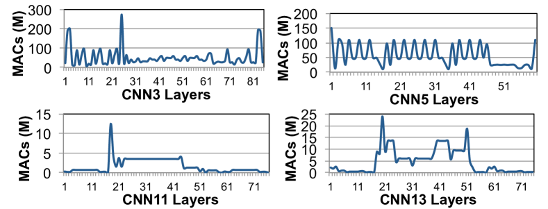
Figure 4: Analysis of number of MAC operation across different layers for four CNN models.

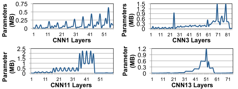
Figure 5: Analysis of parameter footprint across different layers for four CNN models.

Second, we find that layers exhibit significant variation in terms of data reuse patterns for parameters and for input/output activations. For example, a depthwise layer includes only one channel, which leads to very low activation reuse, while a pointwise layer takes in a $1\times K$ filter (K is the depth of the input channel) and convolves it with an input activation across different input channels, leading to much higher activation reuse. We also observe variation in data reuse across layers of the same type. For example, initial/early standard convolution layers in edge CNNs have a shallow input/output channel depth, large input activation width/height, and very small kernels, resulting in very high parameter reuse. In comparison, standard convolution layers that are placed toward the end of the network have a deep input and output channel depth, small input activation width/height, and a large number of kernels, resulting in very low parameter reuse. This variation in reuse is illustrated in Figure 3 (right), which shows that the $\mathrm{FLOP}\text{/}\mathrm{B}$ ratio varies across different layers for five representative CNN models by a factor of 244x.

3.2.3 Analysis of RCNNs

RCNNs include layers from both CNNs and LSTMs. As a result, individual layers from RCNN models exhibit the same characteristics we discussed above for LSTM and CNN layers. We find that layers from RCNNs exhibit on average significantly higher footprints and lower $\mathrm{FLOP}\text{/}\mathrm{B}$ ratios than CNNs, as they include both LSTM and CNN layers. Due to the inclusion of both layer types, we observe significantly more variation across RCNN layers characteristics as well.

3.2.4 Sources of Accelerator Pitfalls

PE Underutilization. We identify three reasons why the Edge TPU falls significantly short of peak throughput. First, while some layers have high parameter reuse (e.g., pointwise layers, with a $1200\text{\,}\mathrm{FLOP}\text{/}\mathrm{B}$ ratio), other layers exhibit very low reuse ($164\text{\,}\mathrm{FLOP}\text{/}\mathrm{B}$) while having large parameter footprints ($0.55\text{\,}\mathrm{MB}\text{/}$). Layers with low reuse yet large footprints for parameters often leave PEs idle, as the parameters incur cache misses to DRAM. The bandwidth of modern commercial DRAM (e.g., $32\text{\,}\mathrm{GB}\text{/}\mathrm{s}$ for LPDDR4 [30]) is two orders of magnitude below the $2\text{\,}\mathrm{TB}\text{/}\mathrm{s}$ bandwidth needed to sustain peak PE throughput when only one $\mathrm{FLOP}\text{/}\mathrm{B}$ is performed (as is the case for LSTM layers). Many (but not all) layers end up with a similar bandwidth problem.

Second, the accelerator does not provide a custom dataflow optimized for each layer. As we identified in Section 3.2, layers both across and within models exhibit high variation in terms of data reuse patterns. This variation necessitates the need for different dataflows for different layers, where each data flow exposes a different set of reuse opportunities for parameters and activations. However, state-of-the-art accelerators such as the Edge TPU employ a single dataflow that is designed for high spatial/temporal reuse [37, 36]. The missed reuse opportunities in many of the model layers causes PEs to needlessly wait on retrieving previously-accessed data that was not properly retained on-chip.

Third, the different shapes and inter-/intra-layer dependencies across different types of layers (e.g., LSTM cell, standard convolution, depthwise, pointwise, fully-connected) makes it challenging to fully utilize a PE array with a fixed size, which is the case in state-of-the-art accelerators [6]. To cater to these differences across layers, there is a need for both better scheduling (e.g., uncovering parallel computation opportunities as we found in Section 3.2.1) and appropriately sizing the PE arrays in order to maintain efficient utilization.

Poor Energy Efficiency. We find three major sources of energy inefficiencies. First, the accelerator incurs high static energy costs because (1) it employs a large overprovisioned on-chip buffer, and (2) it underutilizes PEs. Second, the on-chip buffers consume a high amount of dynamic energy, as we saw for CNN layers in Section 3.1. Third, the accelerator suffers from the high cost of off-chip parameter traffic. On-chip buffers fail to effectively cache parameters for many layers due to layer diversity, causing 50.3% of the total inference energy to be spent on off-chip parameter traffic.

Memory System Issues. We uncover two sources of memory system challenges. First, due to layer diversity, on-chip buffers are ineffective for a large fraction of layers. As we discuss in Section 3.2.1, LSTM gates have large parameter footprints and zero parameter reuse, rendering the on-chip buffer useless for a majority of LSTMs and Transducers, and for a significant fraction of RCNN layers. For CNN layers, we find that those layers with low data reuse account for a significant portion of the entire model parameters (e.g., 64% for CNN6). This means that the on-chip buffer fails to cache a large portion of the parameters for CNN models. As a result, despite being several megabytes in size, the on-chip buffer is effective only for a small fraction of layers, which have an average parameter footprint of only $0.21\text{\,}\mathrm{MB}\text{/}$.

Second, due to having an unnecessarily large on-chip parameter buffer, accesses from those layers with high data reuse become very costly. For those layers, even though they have a small footprint, they perform a large number of buffer accesses. As the on-chip buffer is overprovisioned, the large capacity leads to a high dynamic energy cost per access, even though the capacity is not needed.

3.3 Key Takeaways

Our analysis provides three key insights: (1) there is significant variation in terms of layer characteristics across and within state-of-the-art Google edge models, (2) the monolithic design of the Edge TPU is the root cause of its shortcomings, and (3) to achieve high utilization and energy efficiency, all key components of an edge accelerator (PE array, dataflow, on-chip memory, off-chip memory bandwidth) must be customized based on layer characteristics.

4 MENSA Framework: Key Ideas

Mensa is a new acceleration framework that harnesses layer variation across edge NN models for high efficiency.

4.1 High-Level Overview

Mensa distributes the layers from an NN model across a collection of smaller hardware accelerators that are carefully specialized towards the properties of different layer types. A drawback of current monolithic accelerators is that by designing for a wide range of layers, many of their hardware resources are overprovisioned or introduce high inefficiency. By specializing each accelerator to a subset of layers, Mensa avoids these issues, resulting in an accelerator with a much smaller area that achieves high throughput and efficiency for those layers. Mensa consists of (1) a collection of heterogeneous hardware accelerators; and (2) a runtime scheduler that determines which accelerator each layer in a model should execute on, using a combination of model and hardware characteristics. As we show in Section 5, layers tend to group together into a small number of clusters, allowing designers to typically keep the number of accelerators low.

Mensa is designed as a framework that can support a wide range of architectural implementations. This allows Mensa to be optimized to specific system needs, which is critical to keep resource utilization to a minimum in resource-constrained edge devices, and lets the framework adapt easily to future types of NN models that we expect will arise in the future. We discuss one example implementation of Mensa in Section 5, which caters to the Google edge models that we analyze, to illustrate the effectiveness of our framework.

4.2 Scheduler

The goal of Mensa’s software runtime scheduler is to identify which accelerator each layer in an NN model should run on. Each of the accelerators in Mensa caters to a specific cluster of layers, where the cluster is defined using specific layer characteristics (e.g., type, footprint, data reuse, dependencies). For a given hardware configuration, the scheduler has two pieces of information: (1) the characteristics of each cluster; and (2) which hardware accelerator is best suited for each cluster. Similar to how chipset drivers are configured, this information is generated once during initial setup of a system, and can be modified with an updated driver version to account for new clusters.

When an NN model runs on Mensa, the scheduler generates a mapping between layers and accelerators in Mensa. The scheduler uses the NN model (including a directed acyclic graph that represents communication across model layers) and the configuration information in the driver to determine this mapping. The mapping is generated in two phases.

In the first phase, the scheduler iterates through each layer in the model, and identifies the ideal hardware accelerator for each layer in isolation (i.e., without considering communication overhead). The scheduler determines two properties for each layer: (1) the cluster that the layer belongs to; and (2) the target accelerator for the layer; While this phase works to maximize accelerator throughput and energy efficiency for each layer, the resulting schedule may be sub-optimal for efficiency, because it does not consider the overhead of transferring activations or communicating dependencies (e.g., $h_{t}$ in LSTM cells) between different layers. This can have a large impact on the overall framework performance and energy if the amount of communication is large.

In the second phase, our scheduler accounts for the communication overhead using a simple cost analysis algorithm. For each layer, if the following layer (which we call the subsequent layer) is mapped by the first phase to a different hardware accelerator than the current layer, the algorithm calculates the total amount of data that needs to be communicated between the two layers, and uses a simple heuristic to estimate the total cost of (1) using the phase one mapping (i.e., moving data to the subsequent layer’s accelerator and running that layer on its optimal accelerator), or (2) moving the subsequent layer (i.e., running the subsequent layer on the current layer’s accelerator, which eliminates accelerator-to-accelerator communication, but introduces inefficiencies due to running the subsequent layer on a sub-optimal accelerator). If the cost of moving the subsequent layer is lower than the cost of using the phase one mapping, the subsequent layer is remapped to the current layer’s accelerator.

Once the second phase is complete, Mensa begins model execution using the generated mapping. The scheduler ensures that each layer is executed completely in a single accelerator. Thus, there is no need for intra-layer data synchronization. On the other hand, due to the dependencies between layers, different accelerators may need to communicate with each other. Parameters are read-only and are always fetched from DRAM (i.e., no need for data synchronization). However, activations need to be transferred if two consecutive layers run on different accelerators. Mensa uses DRAM to synchronize activations across accelerators, which avoids the need for sophisticated coherence mechanisms between on-chip and near-data accelerators [4].

5 MENSA for Google Edge Models

We now discuss an example Mensa design optimized for our Google edge models. We start by identifying layer clustering in these models (Section 5.1). Using the unique characteristics for each cluster, we determine which characteristics have the greatest impact on accelerator design, and use that to guide the number of accelerators that we need (Section 5.2).

5.1 Identifying Layer Clusters

We revisit the models that we analyze in Section 3. For each layer, we study the correlation between different characteristics. As an example, Figure 6 shows how the parameter footprint and the number of MAC operations correlate to parameter reuse ($\mathrm{FLOP}\text{/}\mathrm{B}$) for a representative set of layers from five CNNs, two LSTMs, and two Transducers, in order to improve figure clarity. Based on all of the layer characteristics that we analyze, we observe across all layers from all models (not just the representative layers or correlations plotted) that 97% of the layers group into one of five clusters.

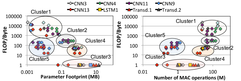
Figure 6: Parameter footprint vs. parameter $\mathrm{FLOP}\text{/}\mathrm{B}$ ratio (left) and number of MAC operations (in millions) vs. parameter $\mathrm{FLOP}\text{/}\mathrm{B}$ ratio (right) across layers.

Cluster 1. Layers in this cluster have (a) a very small parameter footprint ($1100\text{\,}\mathrm{kB}\text{/}$), (b) a very high $\mathrm{FLOP}\text{/}\mathrm{B}$ ratio (780–20K), and (c) high MAC intensity (30M–200M). These layers exhibit high activation footprints and data reuse as well. A majority of layers in this cluster are standard convolution layers with shallow input/output channels and large input activation width/height. We find that these layers are mostly found among early layers in models, and typically achieve high PE utilization (on average 82%).

Cluster 2. Layers in this cluster have (a) a small parameter footprint ($100500\text{\,}\mathrm{kB}\text{/}$; 12x higher on average vs. Cluster 1), (b) a moderate $\mathrm{FLOP}\text{/}\mathrm{B}$ ratio (81–400; up to 10x lower than Cluster 1), and (c) high MAC intensity (20M–100M). They exhibit high activation footprints and activation data reuse as well. Many of the layers belong to pointwise layers, which have high parameter reuse due to convolving 1xK filters (K is input channel depth) with input activation across different channels. Other layers in the cluster include standard convolution layers commonly found in the middle of CNN networks, with deeper input/output channels and smaller activation width/height than the convolution layers in Cluster 1, We find that Cluster 2 layers have lower PE utilization (64%) than layers in Cluster 1.

Cluster 3. Layers in this cluster have (a) a very large parameter footprint ($0.918\text{\,}\mathrm{MB}\text{/}$), (b) minimal parameter reuse, and (c) low MAC intensity (0.1M–10M). These layers exhibit small activation footprints but rather high activation reuse. The majority of these layers are from LSTM gates in LSTMs and Transducers, or are fully-connected layers from CNNs. These layers have very low PE utilization (0.3% on average).

Cluster 4. Layers in this cluster have (a) a larger parameter footprint ($0.52.5\text{\,}\mathrm{MB}\text{/}$), (b) low-to-moderate $\mathrm{FLOP}\text{/}\mathrm{B}$ ratio for parameters (25–64), and (c) moderate MAC intensity (5M–25M). The layers exhibit small activation footprints but rather high activation reuse. A large portion of layers in this category are standard convolution layers with deep input/output channels and input activation width/height, along with a large number of kernels. We find that these layers not only have large parameter footprint, but also include the majority of parameters (up to 64.3%) for their respective model. Cluster 4 layers average a PE utilization of 32%.

Cluster 5. Layers in this cluster have (a) a very small parameter footprint ($1100\text{\,}\mathrm{kB}\text{/}$), (b) a moderate $\mathrm{FLOP}\text{/}\mathrm{B}$ ratio for parameters (49–600), and (c) low MAC intensity (0.5M–5M). The layers exhibit rather high activation footprints but have almost zero activation data reuse. Many of these layers are depthwise layers, which have only one channel (hence the lack of activation reuse), but have high parameter reuse because a small number of filters are convolved across a large input activation (which is the opposite of Cluster 4 layers) Cluster 5 layers achieve a low average PE utilization of 21%.

5.2 Hardware Design Principles

As we study the distinguishing characteristics of each of our five clusters, we find that some characteristics have a strong influence on the hardware design, while others do not necessitate significant changes to the hardware. We discuss two insights that drive our hardware design decisions.

First, we find that MAC intensity and parameter footprint/reuse drive a significant divergence in hardware design, as they impact a number of key accelerator design parameters (e.g., PE array size, on-chip buffer size, memory bandwidth considerations). Looking at our five clusters, we identify that (a) layers in Clusters 1 and 2 share a high MAC intensity, smaller parameter footprint, and moderate-to-high parameter reuse; while (b) layers in Clusters 3 and 4 share a lower MAC intensity, larger parameter footprint, and low parameter reuse. This means that we need at least two different accelerator designs: one that caters to the more compute-centric behavior of Clusters 1/2, and one that caters to the more data-centric behavior of Clusters 3/4. Given our resource-constrained environment, we look to see if layers in Cluster 5, which have a low MAC intensity (similar to Clusters 3 and 4) but a smaller parameter footprint (similar to Clusters 1 and 2), can benefit from one of these two approaches. We find that the low MAC intensity, along with the lower parameter reuse by many Cluster 5 layers, allow the layers to benefit from many of the non-compute-centric optimizations that benefit Clusters 3 and 4, so we consider them together.

Second, a key distinguishing factor between different accelerator designs is the accelerator dataflow, as it dictates which reuse opportunities in layers are exploited, and thus strongly impacts PE utilization and energy efficiency. Prior work [36] analyzes the large dataflow design space, and discusses four types of data reuse: spatial multicasting (reading a parameter once, and spatially distribute it as an input to multiple PEs), temporal multicasting (replicating a parameter in a small local buffer, and delivering the parameter as multiple inputs at different times to the same PE), spatial reduction (accumulating activations from multiple PEs at the same time using multiple compute units), and temporal reduction (accumulating multiple activations generated at different times using a single accumulator/buffer). The chosen dataflow directly affects how the memory system and on-chip network of an accelerator should be designed. Thus, we need different dataflows for clusters with significantly different reuse patterns.

Both of our compute-centric clusters benefit from a similar dataflow, which exposes reuse opportunities for both parameters and activations. Between the compute-centric optimizations and the shared dataflow affinity, we determine that we can use a single accelerator (Pascal) to efficiently execute layers from both Cluster 1 and Cluster 2.

Across our three data-centric clusters, we find that layers from both Clusters 4 and 5 benefit from a dataflow that exposes reuse opportunities for parameters but not for activations, and can thus share an accelerator (Jacquard). Cluster 3 layers exhibit different data reuse characteristics, instead benefitting from a dataflow that provides temporal reduction opportunities for activations. As a result, they need a separate accelerator (Pavlov).

We employ a template-based design approach: while we design each accelerator based on cluster characteristics, we maintain the same generic tiled architecture as the baseline accelerator. We do this to ease the integration of our hardware into a real system: from the perspective of compilers and programs, each of our accelerators appears to be just a different instance (with a different configuration) of the baseline accelerator. This is a critical design decision, as it allows us to deploy and run models using existing highly-optimized design/compile toolchains (e.g., Edge TPU compiler [18]) seamlessly on all of Mensa’s accelerators, with the trade-off of limiting the degree of customization (and, thus, efficiency) our accelerator designs can achieve. While Mensa can work with accelerators that do not employ this tiled architecture, we make this design choice to avoid the need for more complex compilers and multiple libraries for programmers.

5.3 Pascal Accelerator Design

Dataflow. Pascal caters to Cluster 1/2 layers, which have opportunities for both parameter and activation reuse. The layers have a small parameter footprint, which can be captured by a very small on-chip buffer. As a result, exposing reuse opportunities for parameters will likely not provide much additional benefit. The large output activation footprint would require a relatively large buffer to effectively exploit reuse, which would consume significant area and static energy.

If we design our dataflow to provide temporal reduction for the activations, we can significantly reduce the required buffer size while still enabling high reuse (first requirement). However, not all such dataflows can improve efficiency. One example is a dataflow where activations are spatially distributed across PEs, allowing the PEs to collaboratively calculate each output. We should how a pointwise layer (Figure 7a) would map to such a dataflow in Figure 7b. Unfortunately, this dataflow actually worsens the impact of the large output activation footprint, as each output activation is now split into partial sums (one per PE) that need to be gathered and reduced. This reduction generates significant traffic on the on-chip network. We instead want a dataflow that avoids spatial reduction for output activations (second requirement).

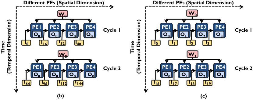
Figure 7: (a) Simplified pointwise layer, (b) an example dataflow that generates high network traffic by spatially reducing output activations, (c) our proposed dataflow.

We develop a dataflow for Pascal that meets both of our design requirements, as shown using a 4-PE toy example in Figure 7c. We spatially distribute output activations, such that each PE calculates one output activation element. This enables temporal reduction for each output activation, and reduces the on-chip buffer size. We replicate each parameter across PEs at each time step (i.e., each PE receives the same parameter), while spatially distributing input activations across PEs. This provides spatial reuse (multicast) for parameters across all PEs in each cycle. Our proposed dataflow generates no partial sum traffic, as the partial sums are instead temporally reduced in each PE’s register file.

PE Array. Layers from Clusters 1 and 2 perform a large number of MAC operations, so we want to size Pascal’s PE array to efficiently perform these in parallel. We analyze the inference latency using different array configurations, and empirically find that a 32x32 array strikes a balance between latency, PE utilization, and energy consumption. In particular, a smaller array increases the latency for Cluster 1 layers, while a larger array provides few benefits. With this array, Pascal achieves a $2\text{\,}\mathrm{TFLOP}\text{/}\mathrm{s}$ peak throughput.

Memory System. The data reuse opportunities exposed by our proposed dataflow enable us to significantly reduce the on-chip buffer sizes, significantly reducing the energy and area costs of Pascal. As we mentioned above, by enabling temporal reduction (in output activations) with our dataflow, we can reduce the size of the on-chip buffer that holds the activations from $2\text{\,}\mathrm{MB}\text{/}$ down to $256\text{\,}\mathrm{kB}\text{/}$. Thanks to the small parameter footprint of layers in Clusters 1 and 2, we can reduce the on-chip parameter buffer by 32x, down to $128\text{\,}\mathrm{kB}\text{/}$.

5.4 Pavlov Accelerator Design

Dataflow. We leverage three characteristics of Cluster 3 layers to shape the design of Pavlov: (1) parameters exhibit zero reuse but have a very large footprint, (2) activations exhibit high reuse but have a small footprint, and (3) the main operation is MVM. Based on these, we identify two design requirements for our dataflow.

First, our dataflow should expose activation reuse opportunities during MVM. One way is using spatial reduction for output activations. However, due to the large parameter footprint (e.g., $W_{h}$ in LSTM cells), this would experience similar issues as we saw for spatial reduction for Clusters 1 and 2 (Section 5.3): there would be a large number of partial sums that need to be combined (as many as one per PE every cycle), resulting in significant network traffic. As a result, we look for more efficient ways to expose activation reuse.

Second, we need to effectively utilize memory bandwidth at low cost. The on-chip buffer is ineffective for these layers, due to the lack of data reuse and the large parameter footprint. As a result, high PE utilization requires many off-chip accesses, and, thus, access to high bandwidth, such as the bandwidth available inside modern 3D-stacked memories. While we want to fully utilize this bandwidth, we cannot do so simply by issuing many outstanding memory requests at once from the accelerator, as this requires complex hardware that often exceeds the area and power budgets available in these memories (and in edge devices) [15, 12, 3]. However, if we can design our dataflow to issue sequential memory accesses to parameters, we can exploit this sequential pattern to use the bandwidth without complex hardware and at a much lower energy cost [15, 12].

Using these requirements, we design our Pavlov dataflow. Output activations are spatially distributed such that each PE is responsible for one output element. Every cycle, the dataflow replicates each input element across all PEs. We use spatial parameter distribution, with each PE receiving a different parameter element during a cycle. Figure 8a shows a toy example of MVM for the forget gate in a LSTM cell, while Figure 8b shows an example of how Pavlov’s dataflow runs that MVM operation on an accelerator with 4 PEs. Each cycle, all of the PEs multiply one input vector element ($X_{0}(t)$ in this example) with a sub-row of $W_{x}$ (or $W_{h}$), storing the partial sum in the PE register file. In the next cycle, the next input element ($X_{1}(t)$) is replicated across all PEs, the next sub-row of parameters is spatially distributed, and the multiply is performed. The product is added to the partial sum sitting in the PE register file (which enables temporal reduction for output activations). After we multiply all rows of the parameter matrix with input vector elements, we obtain the final output activation in each PE.

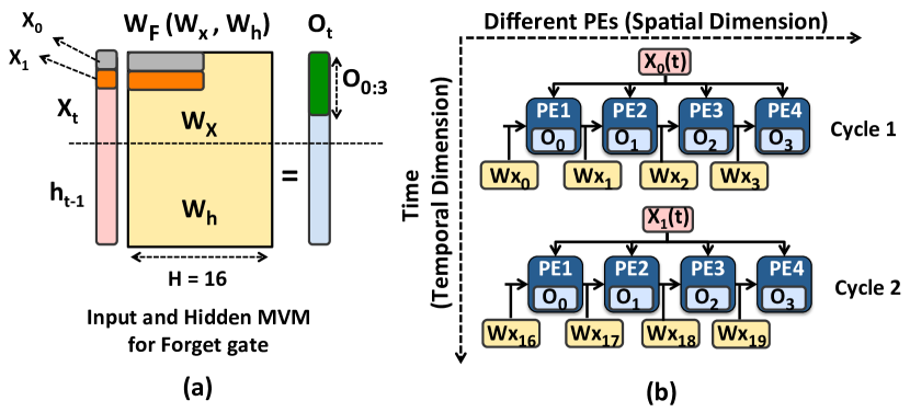
Figure 8: (a) Input/hidden MVMs for a forget gate in a LSTM cell, (b) our proposed dataflow for an LSTM cell.

While the above dataflow is efficient for a single MVM operation, it does not account for inter- and intra-cell dependencies in LSTM layers (the majority of layers in Cluster 3). Not exploiting reuse opportunities for these dependencies can be costly (e.g., for a 100-sequence input, where $W_{x}$ and $W{h}$ are both 1000x1000, each layer would generate $500\text{\,}\mathrm{MB}\text{/}$ of off-chip parameter traffic). $W_{x}$ and $W_{h}$ elements are reused across LSTM cells within a layer (e.g., $W_{hf}$ is reused across all cells in Figure 9a). While these arrays are too large to cache, we can decouple the computation of input and hidden MVM in each gate, and calculate all input MVMs for all cells ahead of time (as they have no dependencies across cells). This allows us to fetch $W_{hf}$ elements only once from memory. We can later perform the hidden MVM computations while respecting their inter-cell dependencies.

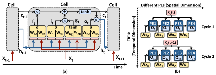
Figure 9: (a) LSTM layer internal structure, (b) our LSTM cell dataflow optimized to exploit dependencies.

We modify our dataflow, as shown in Figure 9b, to efficiently reuse $W_{x}$ and $W_{h}$. Now, when we fetch and spatially distribute a sub-row of $W_{x}$ across PEs, we keep those parameters in the PE register file. Each iteration, every PE multiplies one element of $x_{t}$ ($x_{0}(t)$ in Figure 9b) and one element of the $W_{x}$ sub-row. Now, instead of going to the next sub-row, we fetch the next input element ($x_{0}(t+1)$ in Figure 9b) and perform the MVM for another LSTM cell. Note that instead of accumulating only a single partial sum in each PE’s register file, we accumulate $K$ partial sums, one for each LSTM cell being computed concurrently. With this dataflow, we eliminate the need to fetch $W_{x}$ more than once from DRAM.

PE Array. Because Cluster 3 layers have a low MAC intensity, and mainly perform MVM, we design a much smaller PE array for Pavlov than that in the baseline accelerator. We again analyze the inference latency across a range of PE array sizes, and find that an 8x8 array ($128\text{\,}\mathrm{GFLOP}\text{/}\mathrm{s}$ peak throughput) balances latency, utilization, and energy.

Memory System. Since Pavlov is data-centric and its sequential memory accesses exploit high memory bandwidth, we place it in the logic layer of a 3D-stacked memory, where the bandwidth is much higher than the external bandwidth to the CPU. Given that parameters and activations from these layers exhibit different characteristics, we customize separate on-chip buffers for each data type. For parameters, we use only one level of memory hierarchy ($512\text{\,}\mathrm{B}\text{/}$ private buffer per PE) and stream parameters directly from DRAM, as (1) their minimal reuse and large footprint does not warrant a shared on-chip buffer, (2) our proposed dataflow now generates sequential accesses that can efficiently utilize the full memory bandwidth. For activations, thanks to the small activation footprint of layers in Cluster 3, we use a $128\text{\,}\mathrm{kB}\text{/}$ buffer.

5.5 Jacquard Accelerator Design

Dataflow. We leverage three characteristics of Cluster 4/5 layers to shape the design of Jacquard: (1) activations exhibit very low reuse; (2) parameters exhibit lower reuse than Cluster 1/2 layers, but exhibit much higher reuse than activations; and (3) the footprint of activations is low for all layers, while the parameter footprint is high for many (but not all) layers. Based on these, we need to design a dataflow that exposes reuse opportunities for parameters, which in turn allows us to shrink the on-chip parameter buffer.

There are several variations of dataflows that can enable reuse opportunities for parameters. For example, we can replicate the same parameter across different PEs, and temporally reuse parameter across different iterations. For each parameter, this results in a reuse factor (i.e., the number of cycles a parameter is reused) of $WxH/N$, where $N$ is the number of PEs and $WxH$ is the dimension of the output activations. Once we traverse all $WxH$ output activations, we need to broadcast a new parameter element across the PEs and repeat the process. If the output activation dimension is small (which is the case for Cluster 4/5 layers), the reuse factor for each parameter becomes too small, resulting in frequent parameter broadcasting. This is particularly problematic for Cluster 4 layers, which often have a large number of filters (i.e., a large parameter footprint). The on-chip traffic generated by frequent parameter broadcasting prevents us from efficiently overlapping the retrieval of parameters from DRAM with PE computation, leading to PE underutilization.

To avoid this in Jacquard, we instead spatially distribute parameters across PEs. All PEs collaboratively calculate one output activation, while input activations are spatially distributed among PEs. The parameters stay in the PE register file across different cycles (temporal reuse) until we traverse the all of the output activations. This increases the reuse factor to $WxH$ and reduces on-chip traffic (by eliminating the parameter broadcasts). With this larger reuse factor, our dataflow can now effectively hide the DRAM access latency with PE computation time.

PE Array. While Cluster 4/5 layers have a low MAC intensity, they perform more MAC operations on average than Cluster 3 layers. Our analysis of PE array sizes shows that equipping Jacquard with an array smaller than 16x16 increases the latency, so we select 16x16 for the array size. This allows Jacquard to achieve a peak throughput of $512\text{\,}\mathrm{GFLOP}\text{/}\mathrm{s}$.

Memory System. Similar to Pavlov, we decide to place Jacquard inside the logic layer of 3D-stacked memory. This provides high bandwidth for the large parameter footprints of Cluster 4 layers. We use separate shared buffers for each data type. Given the small activation footprints, we use a small $128\text{\,}\mathrm{kB}\text{/}$ buffer for them (a 16x reduction compared to the baseline accelerator). Our proposed dataflow for Jacquard enables Thanks to the temporal parameter reuse across iterations that our dataflow enables, we can reduce the parameter buffer size by 32x (down to $128\text{\,}\mathrm{kB}\text{/}$) over the Edge TPU.

6 Experimental Methodology

Models & Simulation. The Google edge NN models that we analyze are used in several Google mobile applications/products, such as image classification, object detection, semantic segmentation, automatic speech recognition, and image captioning. The models are specifically developed for edge devices using TensorFlow Lite [19], and are fully 8-bit quantized using quantization-aware training [20]. The models are then compiled using the Edge TPU compiler [18].

Energy Analysis. We build our energy model based on prior works [3, 15, 4], which sums up the total energy consumed by the accelerator, DRAM, off-chip and on-chip interconnects, and all on-chip buffers. We use CACTI-P 6.5 [40] with a $22\text{\,}\mathrm{nm}\text{/}$ process technology to estimate on-chip buffer energy. We assume that each 8-bit MAC unit consumes $0.2\text{\,}\mathrm{pJ}\text{/}\mathrm{bit}$. We model the DRAM energy as the energy consumed per bit for LPDDR4, based on models from prior works [15, 3].

Performance Analysis. We use an in-house simulator to model all major components of the Edge TPU, including the PE array, memory system, on-chip network, and dataflow. We heavily modify the simulator to implement our three proposed accelerators and the software runtime of Mensa. We develop an analytical cost model to determine the performance of each of our proposed dataflows, and integrate the dataflow performance numbers into our simulator’s performance model. We use CACTI-P 6.5 [40] to determine the on-chip buffer latencies for each proposed accelerator. Similar to prior works [3, 15, 12, 4], the accelerators in the logic layer of 3D-stacked memory have access to the $256\text{\,}\mathrm{GB}\text{/}\mathrm{s}$ internal bandwidth of High-Bandwidth Memory (HBM) [29], which is 8x the bandwidth to accelerators that sit outside of memory.

7 Evaluation

We evaluate energy and performance for four configurations: (1) Baseline, the Edge TPU; (2) Base+HB, a hypothetical version of Baseline with 8x bandwidth ($256\text{\,}\mathrm{GB}\text{/}\mathrm{s}$); (3) EyerissV2, a state-of-the-art edge accelerator [6] that uses reconfigurable interconnects to address CNN model heterogeneity; and (4) our implementation of Mensa with all three proposed accelerators (Pascal, Pavlov, Jacquard). To improve figure clarity, we show individual model results for only a few representative models of each model type. Our average results are reported across all 24 Google edge models.

7.1 Inference Energy Analysis

Figure 10 (left) shows the total inference energy across different NN models by our four configurations. We make three observations from the figure.

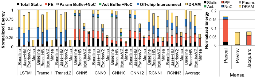
Figure 10: Inference energy across different models (left) and energy breakdown across our three proposed accelerators (right), normalized to Baseline.

First, providing high bandwidth to Baseline results in only a small reduction (7.5% on average) of inference energy. This is because Base+HB still incurs the high energy costs of (1) on-chip buffers that are overprovisioned for many layers, and (2) off-chip traffic to DRAM. Base+HB benefits LSTMs and Transducers the most (14.2% energy reduction), as the higher bandwidth significantly reduces the inference latency of these models, which in turn lowers static energy.

Second, EyerissV2 suffers from significant energy inefficiency for LSTMs and Transducers. While EyerissV2 lowers static energy compared to Baseline, due to its use of a much smaller PE array (384 vs. 4096) and on-chip buffers ($192\text{\,}\mathrm{kB}\text{/}$ vs. $4\text{\,}\mathrm{MB}\text{/}$), it still incurs the high energy costs of off-chip parameter traffic to DRAM. Averaged across all LSTM and Transducer models, EyerissV2 reduces energy by only 6.4% over Baseline. For CNN models, EyerissV2 reduces inference energy by 36.2% over Baseline, as its smaller on-chip buffer significantly reduces dynamic energy consumption.

Third, Mensa significantly reduces inference energy across all models. The reduction primarily comes from three sources. (1) Mensa lowers the energy spent on on-chip and off-chip parameter traffic by 15.3x, by scheduling layers on the accelerators with the most appropriate dataflow for each layer. LSTMs and Transducers benefit the most, as their inference energy in both Base+HB and EyerissV2 is dominated by off-chip parameter traffic, which Pavlov and Jacquard drastically cut due to being placed inside memory. (2) Mensa reduces the dynamic energy of the on-chip buffer and network (NoC) by 49.8x and 6.2x over Base+HB and EyerissV2, by avoiding overprovisioning and catering to specialized dataflows. This is most beneficial for CNN and RCNN models. (3) Mensa reduces static energy by 3.6x and 5.6x over Base+HB and EyerissV2, thanks to using significantly smaller PE arrays that avoid underutilization, significantly smaller on-chip buffers, and dataflows that reduce inference latency.

EyerissV2 falls significantly short (50.6%) of Mensa’s energy efficiency for three reasons. First, while EyerissV2’s flexible NoC can provide a high data rate to the PE array, its fixed dataflow cannot efficiently expose reuse opportunities across different layers (e.g., Cluster 4 and 5 layers that have very large parameter footprints and low data reuse). Second, EyerissV2 has much higher static energy consumption, as its inference latency is significantly larger for many compute-intensive CNN layers (as its PE array is much smaller than the array in Pascal). Third, some CNN layers have a large parameter footprint and very low data reuse, which generates a large amount of off-chip parameter traffic in EyerissV2. Overall, Mensa reduces total inference energy by 66.0%/50.6%, and improves energy efficiency ($\mathrm{TFLOP}\text{/}\mathrm{J}$) by 3.0x/2.4x, compared to Baseline/EyerissV2.

Figure 10 (right) shows the breakdown of energy usage across our three Mensa accelerators. Pascal consumes the most energy of the three, with its consumption dominated by the PE array (since the layers that run on Pascal perform a large number of MAC operations). Pavlov’s energy usage is dominated by DRAM accesses, as its layers have large footprints and no data reuse. For Jacquard, the majority of energy is used by a combination of DRAM accesses and the PE array, but the usage is lower than Pavlov DRAM accesses or the Pascal PE array due to the inherent layer properties (smaller footprints, lower MAC intensity).

7.2 Performance Analysis

Figure 11 shows the utilization (bars, left axis) and throughput (lines, right axis) for our four configurations. Mensa’s utilization is calculated by computing the average utilization across its three accelerators (Pascal, Pavlov and Jacquard). We make three observations from the figure.

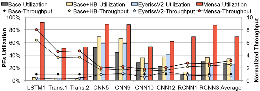
Figure 11: Accelerator utilization and throughput across different models, normalized to Baseline.

First, Baseline suffers from low PE array utilization (on average 27.3%). The higher bandwidth in Base+HB pushes average utilization up to 34.0%, and improves throughput by 2.5x. The largest improvements are for LSTMs and Transducers (4.5x on average vs. 1.3x for CNNs), thanks to their low $\mathrm{FLOP}\text{/}\mathrm{B}$ ratio and large footprints. In contrast, some CNN models (e.g., CNN10) see only modest improvements (11.7%) with Base+HB, as their layers have high reuse and small footprints. Overall, Base+HB still has very low utilization, as many layers (those from Clusters 3, 4, and 5) do not need the large number of PEs in the accelerator.

Second, EyerissV2 reduces performance significantly over Baseline for several models. EyerissV2’s flexible interconnect and much smaller PE array do allow it to achieve slightly higher PE utilization than Baseline for layers that have very low data reuse. However, this higher utilization is offset by significantly higher inference latencies. For compute-intensive layers in Clusters 1 and 2, the smaller PE array size hurts layer throughput. For data-centric layers in Clusters 4 and 5, EyerissV2 cannot customize its dataflow to expose reuse opportunities, and thus is hurt by the high off-chip traffic. Overall, we find that EyerissV2’s overall throughput is actually lower than Baseline for most of our models.

Third, Mensa provides a significant increase in both average utilization (2.5x/2.0x/2.6x) and throughput (3.1x/1.3x/4.3x) over Baseline/Base+HB/EyerissV2. The large utilization improvements are a result of (1) properly-provisioned PE arrays for each layer, (2) customized dataflows that exploit reuse and opportunities for parallelization, and (3) the movement of large-footprint layer computation into memory (eliminating off-chip traffic for their DRAM requests). We note that Mensa’s throughput improvements over Base+HB are smaller than its utilization improvements, because Base+HB is reasonably effective at reducing the inference latency of layers with poor reuse and large footprints (albeit with poor energy efficiency and underutilization). Mensa benefits all NN model types, but the largest improvements are for LSTMs and Transducers, with average utilization/throughput improvements of 82.0x/5.7x over Baseline. The improvement is lower for CNNs and RCNNs (2.23x/1.8x over Baseline), because they make more use of Baseline’s large PE arrays, and have smaller footprints that lessen the impact of off-chip DRAM accesses. For a few CNNs (CNN10–CNN13), their utilization is somewhat lower than desired (44.7%) due to their use of a large number of depthwise layers (part of Cluster 5) that have significantly lower data reuse than other Cluster 4/5 layers. While these layers run less optimally with Jacquard’s dataflow due to the different reuse behavior, Mensa still improves their utilization by 65.2% over Baseline because Jacquard’s specialization still helps depthwise layers.

Figure 12 shows the overall inference latency, and where the inference latency in Mensa is spent (across Pascal, Pavlov, and Jacquard). We find that Mensa outperforms Baseline and Base+HB on average by 1.96x and 1.17x. LSTMs and Transducers see a significant latency reduction with Mensa (5.4x/1.26x vs. Baseline/Base+HB) because most of their layers run on Pavlov and benefit from an optimized dataflow and processing-in-memory (which provides not only higher bandwidth, but also lower latency for DRAM accesses). CNNs and RCNNs benefit from the heterogeneity of our accelerators, making use of all three of them to reduce latency by 1.64x/1.16x over Baseline/Base+HB.

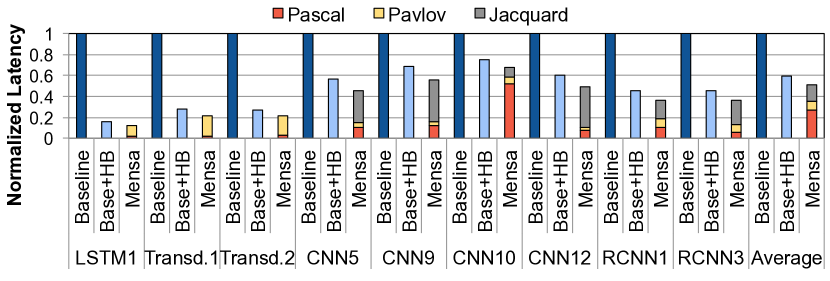
Figure 12: Inference latency, normalized to Baseline.

8 Related Work

To our knowledge, this is the first work to (1) examine the bottlenecks of a state-of-the-art commercial Google Edge TPU when executing state-of-the-art Google edge NN models; (2) quantify the significant layer variation that exists in state-of-the-art edge NN models; (3) identify that layers can be clustered together based on a number of shared characteristics; (4) propose a new framework for heterogeneous ML inference acceleration (Mensa), with both on-chip and near-data accelerators; and (5) provide an example heterogeneous accelerator design for Google edge NN models.

Many prior works [48, 7, 15, 6, 13, 57, 23, 51, 50, 22, 46, 33, 1, 2, 5, 39, 42, 45] look at a specific model type (predominantly CNNs). None of these works perform an analysis across different classes of edge models (e.g., Transducers, LSTMs, RCNNs). In fact, many of them (e.g., [7, 15, 13, 45, 42]) analyze traditional models (e.g., AlexNet, VGG), and their proposals are not tailored toward state-of-the-art edge models (which we show are different) or resource-limited edge devices. These proposals cater accelerators toward a particular model type (e.g., CNNs [7, 15, 50, 46, 42], LSTMs [48, 57]), and they are not optimized to serve multiple model types. As a result, they all suffer from the issues we discuss in Section 3.

Some CNN-focused works observe diversity across CNN layers [36, 51, 6, 37, 32, 45]. Maeri [37] and Eyeriss v2 [6] use reconfigurable logic to provide flexible dataflows and networks for different layers. However, those solutions (1) cannot reconfigure a number of essential design parameters, (2) require frequent online reconfiguration to cater to edge layer variation, and (3) make it difficult to co-design the dataflow with key components such as the memory system. We quantitatively compare Eyeriss v2 to Mensa in Section 7. ScaleDeep [51] proposes customized processing tiles to address diversity in CNN layers. While the idea shares some similarities with Mensa (exploiting heterogeneity in hardware), ScaleDeep (1) targets traditional cloud-based training instead of edge inference, resulting in significantly different support for diversity; and (2) does not address the larger diversity that exists between CNN layers and layers in other model types (e.g., LSTM layers). Neurosurgeon [32] looks at both vision and speech models. However, their analysis is done on old/traditional vision/speech models, and their solution relies on offloading some layers to the cloud, which undermines the goal of running inference locally.

9 Conclusion

We conduct the first bottleneck analysis of the Google Edge TPU, a state-of-the-art ML inference accelerator, as it executes 24 state-of-the-art Google edge NN models. Our analysis reveals that the Edge TPU’s monolithic design leads to significant underutilization and poor energy efficiency for our edge NN models, which exhibit significant layer variation. We propose a new framework called Mensa, consisting of multiple small heterogeneous accelerators, each specialized to specific layer characteristics. Using our discovery that layers group into a small number of clusters, we create a Mensa design for the Google edge NN models consisting of three accelerators. Compared to the Edge TPU and to a state-of-the-art reconfigurable ML accelerator, our design improves energy efficiency by 3.0x/2.4x and throughput by 3.1x/4.3x for our edge NN models. We hope that Mensa can enable the design and adoption of future heterogeneous accelerators that support yet-to-be-developed NN model types.

References

- [1] J. Albericio, P. Judd, T. Hetherington, T. Aamodt, N. E. Jerger, and A. Moshovos, “Cnvlutin: Ineffectual-neuron-free deep neural network computing,” in ISCA, 2016.
- [2] M. Alwani, H. Chen, M. Ferdman, and P. Milder, “Fused-layer cnn accelerators,” in MICRO, 2016.
- [3] A. Boroumand, S. Ghose, Y. Kim, R. Ausavarungnirun, E. Shiu, R. Thakur, D. Kim, A. Kuusela, A. Knies, P. Ranganathan, and O. Mutlu, “Google Workloads for Consumer Devices: Mitigating Data Movement Bottlenecks,” in ASPLOS, 2018.
- [4] A. Boroumand, S. Ghose, M. Patel, H. Hassan, B. Lucia, R. Ausavarungnirun, K. Hsieh, N. Hajinazar, K. T. Malladi, H. Zheng, and O. Mutlu, “CoNDA: Efficient Cache Coherence Support for Near-data Accelerators,” in ISCA, 2019.
- [5] T. Chen, Z. Du, N. Sun, J. Wang, C. Wu, Y. Chen, and O. Temam, “Diannao: A small-footprint high-throughput accelerator for ubiquitous machine-learning,” in ASPLOS, 2014.
- [6] Y. Chen, T. Yang, J. Emer, and V. Sze, “Eyeriss v2: A flexible accelerator for emerging deep neural networks on mobile devices,” JETCAS, 2019.
- [7] Y. H. Chen, T. Krishna, J. S. Emer, and V. Sze, “Eyeriss: An Energy-Efficient Reconfigurable Accelerator for Deep Convolutional Neural Networks,” JSSC, 2017.
- [8] J. W. Choi, D. Bedard, R. Fowler, and R. Vuduc, “A roofline model of energy,” in IPDPS, 2013.
- [9] K. Choi, G. Fazekas, M. Sandler, and K. Cho, “Convolutional recurrent neural networks for music classification,” in ICASSP, 2017.
- [10] J. Chung, C. Gulcehre, K. Cho, and Y. Bengio, “Empirical evaluation of gated recurrent neural networks on sequence modeling,” in NIPS, 2014.
- [11] J. Donahue, L. Anne Hendricks, S. Guadarrama, M. Rohrbach, S. Venugopalan, K. Saenko, and T. Darrell, “Long-term recurrent convolutional networks for visual recognition and description,” in CVPR, 2015.
- [12] M. Drumond, A. Daglis, N. Mirzadeh, D. Ustiugov, J. Picorel, B. Falsafi, B. Grot, and D. Pnevmatikatos, “The Mondrian Data Engine,” in ISCA, 2017.
- [13] Z. Du, R. Fasthuber, T. Chen, P. Ienne, L. Li, T. Luo, X. Feng, Y. Chen, and O. Temam, “ShiDianNao: Shifting vision processing closer to the sensor,” in ISCA, 2015.
- [14] J. Fowers, K. Ovtcharov, M. Papamichael, T. Massengill, M. Liu, D. Lo, S. Alkalay, M. Haselman, L. Adams, M. Ghandi, S. Heil, P. Patel, A. Sapek, G. Weisz, L. Woods, S. Lanka, S. K. Reinhardt, A. M. Caulfield, E. S. Chung, and D. Burger, “A configurable cloud-scale dnn processor for real-time ai,” in ISCA, 2018.
- [15] M. Gao, J. Pu, X. Yang, M. Horowitz, and C. Kozyrakis, “TETRIS: Scalable and Efficient Neural Network Acceleration with 3D Memory,” in ASPLOS, 2017.
- [16] M. Gao, X. Yang, J. Pu, M. Horowitz, and C. Kozyrakis, “Tangram: Optimized coarse-grained dataflow for scalable nn accelerators,” in ASPLOS, 2019.
- [17] Google LLC, “Edge TPU.” [Online]. Available: https://cloud.google.com/edge-tpu
- [18] Google LLC, “Edge TPU Compiler,” https://coral.ai/docs/edgetpu/compiler/.
- [19] Google LLC, “TensorFlow Lite,” https://www.tensorflow.org/lite/.
- [20] Google LLC, “TensorFlow Models on the Edge TPU,” https://coral.ai/docs/edgetpu/models-intro/.
- [21] A. Graves, “Sequence transduction with recurrent neural networks,” arXiv, 2012. [Online]. Available: http://arxiv.org/abs/1211.3711
- [22] S. Gudaparthi, S. Narayanan, R. Balasubramonian, E. Giacomin, H. Kambalasubramanyam, and P.-E. Gaillardon, “Wire-aware architecture and dataflow for cnn accelerators,” in MICRO, 2019.
- [23] U. Gupta, B. Reagen, L. Pentecost, M. Donato, T. Tambe, A. M. Rush, G. Wei, and D. Brooks, “Masr: A modular accelerator for sparse rnns,” in PACT, 2019.
- [24] Y. He, T. N. Sainath, R. Prabhavalkar, I. McGraw, R. Alvarez, D. Zhao, D. Rybach, A. Kannan, Y. Wu, R. Pang, Q. Liang, D. Bhatia, Y. Shangguan, B. Li, G. Pundak, K. C. Sim, T. Bagby, S. Chang, K. Rao, and A. Gruenstein, “Streaming end-to-end speech recognition for mobile devices,” in ICASSP, 2019.
- [25] A. G. Howard, M. Zhu, B. Chen, D. Kalenichenko, W. Wang, T. Weyand, M. Andreetto, and H. Adam, “Mobilenets: Efficient convolutional neural networks for mobile vision applications,” 2017.
- [26] F. N. Iandola, S. Han, M. W. Moskewicz, K. Ashraf, W. J. Dally, and K. Keutzer, “Squeezenet: Alexnet-level accuracy with 50x fewer parameters and <0.5mb model size,” 2016.
- [27] Intel Corp., “Intel Movidius Neural Compute Stick.” [Online]. Available: https://software.intel.com/content/www/us/en/develop/articles/intel-movidius-neural-compute-stick.html
- [28] M. H. Ionica and D. Gregg, “The movidius myriad architecture’s potential for scientific computing,” IEEE Micro, 2015.
- [29] JEDEC Solid State Technology Assn., “JESD235B: High Bandwidth Memory (HBM) DRAM,” December 2018.
- [30] JEDEC Solid State Technology Assn., “JESD209-4C: Low Power Double Data Rate 4 (LPDDR4) Standard,” January 2020.
- [31] N. P. Jouppi, C. Young, N. Patil, D. Patterson, G. Agrawal, R. Bajwa, S. Bates, S. Bhatia, N. Boden, A. Borchers, R. Boyle, P. luc Cantin, C. Chao, C. Clark, J. Coriell, M. Daley, M. Dau, J. Dean, B. Gelb, T. V. Ghaemmaghami, R. Gottipati, W. Gulland, R. Hagmann, C. R. Ho, D. Hogberg, J. Hu, R. Hundt, D. Hurt, J. Ibarz, A. Jaffey, A. Jaworski, A. Kaplan, H. Khaitan, A. Koch, N. Kumar, S. Lacy, J. Laudon, J. Law, D. Le, C. Leary, Z. Liu, K. Lucke, A. Lundin, G. MacKean, A. Maggiore, M. Mahony, K. Miller, R. Nagarajan, R. Narayanaswami, R. Ni, K. Nix, T. Norrie, M. Omernick, N. Penukonda, A. Phelps, J. Ross, M. Ross, A. Salek, E. Samadiani, C. Severn, G. Sizikov, M. Snelham, J. Souter, D. Steinberg, A. Swing, M. Tan, G. Thorson, B. Tian, H. Toma, E. Tuttle, V. Vasudevan, R. Walter, W. Wang, E. Wilcox, and D. H. Yoon, “In-datacenter performance analysis of a tensor processing unit,” in ISCA, 2017.
- [32] Y. Kang, J. Hauswald, C. Gao, A. Rovinski, T. Mudge, J. Mars, and L. Tang, “Neurosurgeon: Collaborative intelligence between the cloud and mobile edge,” in ASPLOS, 2017.
- [33] L. Ke, U. Gupta, B. Y. Cho, D. Brooks, V. Chandra, U. Diril, A. Firoozshahian, K. Hazelwood, B. Jia, H. S. Lee, M. Li, B. Maher, D. Mudigere, M. Naumov, M. Schatz, M. Smelyanskiy, X. Wang, B. Reagen, C. Wu, M. Hempstead, and X. Zhang, “Recnmp: Accelerating personalized recommendation with near-memory processing,” in ISCA, 2020.
- [34] A. Khamparia, B. Pandey, S. Tiwari, D. Gupta, A. Khanna, and J. Rodrigues, “An integrated hybrid CNN–RNN model for visual description and generation of captions,” Circuits, Systems, and Signal Processing, 2019.
- [35] A. Krizhevsky, I. Sutskever, and G. E. Hinton, “Imagenet classification with deep convolutional neural networks,” CACM, 2017.
- [36] H. Kwon, P. Chatarasi, M. Pellauer, A. Parashar, V. Sarkar, and T. Krishna, “Understanding Reuse, Performance, and Hardware Cost of DNN Dataflow: A Data-Centric Approach,” in MICRO, 2019.
- [37] H. Kwon, A. Samajdar, and T. Krishna, “MAERI: Enabling Flexible Dataflow Mapping over DNN Accelerators via Reconfigurable Interconnects,” in ASPLOS, 2018.
- [38] J. Li, R. Zhao, H. Hu, and Y. Gong, “Improving rnn transducer modeling for end-to-end speech recognition,” in ASRU, 2019.
- [39] W. Lu, G. Yan, J. Li, S. Gong, Y. Han, and X. Li, “Flexflow: A flexible dataflow accelerator architecture for convolutional neural networks,” in HPCA, 2017.
- [40] N. Muralimanohar, R. Balasubramonian, and N. Jouppi, “Optimizing NUCA Organizations and Wiring Alternatives for Large Caches with CACTI 6.0,” in MICRO, 2007.
- [41] NVIDIA Corp., “NVIDIA Jetson Nano.” [Online]. Available: https://developer.nvidia.com/embedded/jetson-nano-developer-kit
- [42] A. Parashar, M. Rhu, A. Mukkara, A. Puglielli, R. Venkatesan, B. Khailany, J. Emer, S. W. Keckler, and W. J. Dally, “Scnn: An accelerator for compressed-sparse convolutional neural networks,” in ISCA, 2017.
- [43] K. Rao, H. Sak, and R. Prabhavalkar, “Exploring architectures, data and units for streaming end-to-end speech recognition with rnn-transducer,” 2018.
- [44] H. Sak, A. W. Senior, and F. Beaufays, “Long Short-Term Memory Based Recurrent Neural Network Architectures for Large Vocabulary Speech Recognition,” arXiv, 2014.
- [45] Y. S. Shao, J. Clemons, R. Venkatesan, B. Zimmer, M. Fojtik, N. Jiang, B. Keller, A. Klinefelter, N. Pinckney, P. Raina, S. G. Tell, Y. Zhang, W. J. Dally, J. Emer, C. T. Gray, B. Khailany, and S. W. Keckler, “Simba: Scaling deep-learning inference with multi-chip-module-based architecture,” in MICRO, 2019.
- [46] Y. Shen, M. Ferdman, and P. Milder, “Maximizing cnn accelerator efficiency through resource partitioning,” in ISCA, 2017.
- [47] D. Shin, J. Lee, J. Lee, and H. Yoo, “14.2 DNPU: An 8.1TOPS/W Reconfigurable CNN-RNN Processor for General-Purpose Deep Neural Networks,” in ISSCC, 2017.
- [48] F. Silfa, G. Dot, J.-M. Arnau, and A. Gonzàlez, “E-PUR: An Energy-Efficient Processing Unit for Recurrent Neural Networks,” in PACT, 2018.
- [49] K. Simonyan and A. Zisserman, “Very Deep Convolutional Networks for Large-Scale Image Recognition,” in ICLR, 2015.
- [50] F. Tu, W. Wu, S. Yin, L. Liu, and S. Wei, “RANA: Towards Efficient Neural Acceleration with Refresh-Optimized Embedded DRAM,” in ISCA, 2018.
- [51] S. Venkataramani, A. Ranjan, S. Banerjee, D. Das, S. Avancha, A. Jagannathan, A. Durg, D. Nagaraj, B. Kaul, P. Dubey, and A. Raghunathan, “SCALEDEEP: A Scalable Compute Architecture for Learning and Evaluating Deep Networks,” in ISCA, 2017.
- [52] O. Vinyals, A. Toshev, S. Bengio, and D. Erhan, “Show and tell: A neural image caption generator,” in CVPR, 2015.
- [53] C. Wu, D. Brooks, K. Chen, D. Chen, S. Choudhury, M. Dukhan, K. Hazelwood, E. Isaac, Y. Jia, B. Jia, T. Leyvand, H. Lu, Y. Lu, L. Qiao, B. Reagen, J. Spisak, F. Sun, A. Tulloch, P. Vajda, X. Wang, Y. Wang, B. Wasti, Y. Wu, R. Xian, S. Yoo, and P. Zhang, “Machine learning at facebook: Understanding inference at the edge,” in HPCA, 2019.
- [54] Y. Wu, M. Schuster, Z. Chen, Q. V. Le, M. Norouzi, W. Macherey, M. Krikun, Y. Cao, Q. Gao, K. Macherey, J. Klingner, A. Shah, M. Johnson, X. Liu, L. Kaiser, S. Gouws, Y. Kato, T. Kudo, H. Kazawa, K. Stevens, G. Kurian, N. Patil, W. Wang, C. Young, J. Smith, J. Riesa, A. Rudnick, O. Vinyals, G. S. Corrado, M. Hughes, and J. Dean, “Google’s neural machine translation system: Bridging the gap between human and machine translation,” ArXiv, 2016.
- [55] X. Xu, Y. Ding, S. X. Hu, M. T. Niemier, J. Cong, Y. Hu, and Y. Shi, “Scaling for edge inference of deep neural networks,” Nature Electronics, vol. 1, pp. 216–222, 2018.
- [56] X. Zhang, X. Liu, A. Ramachandran, C. Zhuge, S. Tang, P. Ouyang, Z. Cheng, K. Rupnow, and D. Chen, “High-performance video content recognition with long-term recurrent convolutional network for fpga,” in FPL, 2017.
- [57] T. Zhao, Y. Zhang, and K. Olukotun, “Serving recurrent neural networks efficiently with a spatial accelerator,” ArXiv, 2019.