Towards Enhancing Database Education: Natural Language Generation Meets Query Execution Plans

Abstract.

The database systems course is offered as part of an undergraduate computer science degree program in many major universities. A key learning goal of learners taking such a course is to understand how sql queries are processed in a rdbms in practice. Since a query execution plan (qep) describes the execution steps of a query, learners can acquire the understanding by perusing the qeps generated by a rdbms. Unfortunately, in practice, it is often daunting for a learner to comprehend these qeps containing vendor-specific implementation details, hindering her learning process. In this paper, we present a novel, end-to-end, generic system called lantern that generates a natural language description of a qep to facilitate understanding of the query execution steps. It takes as input an sql query and its qep, and generates a natural language description of the execution strategy deployed by the underlying rdbms. Specifically, it deploys a declarative framework called pool that enables subject matter experts to efficiently create and maintain natural language descriptions of physical operators used in qeps. A rule-based framework called rule-lantern is proposed that exploits pool to generate natural language descriptions of qeps. Despite the high accuracy of rule-lantern, our engagement with learners reveal that, consistent with existing psychology theories, perusing such rule-based descriptions lead to boredom due to repetitive statements across different qeps. To address this issue, we present a novel deep learning-based language generation framework called neural-lantern that infuses language variability in the generated description by exploiting a set of paraphrasing tools and word embedding. Our experimental study with real learners shows the effectiveness of lantern in facilitating comprehension of qeps.

1. Introduction

There is continuous demand for database-literate professionals in today’s market due to the widespread usage of relational database management system (rdbms) in the commercial world. Such commercial demand has played a pivotal role in the offering of database systems course as part of an undergraduate computer science (cs) degree program in major universities around the world. Furthermore, not all working adults dealing with rdbms have taken an undergraduate database course. Hence, they often need to undergo on-the-job training or attend relevant courses in higher institutes of learning to acquire database literacy. Indeed, while formal education for young learners at universities has been the focus of educational provisions in the industrial age, the digital age is now seeing an increased experimentation of “lifelong learning” (unesco, ) with provisions such as work-study programmes for early career and mid-career individuals, and digital learning initiatives.

A key learning goal of learners taking a database course is to understand how sql queries are processed in a rdbms in practice. A relational query engine produces a query execution plan (qep), which represents an execution strategy of an sql query. Hence, such understanding can be gained by learners by perusing the qeps of queries. Major database textbooks introduce the general (i.e., not tied to any specific rdbms software) theories and principles behind the generation of qeps using natural language-based narratives and visual examples. This allows a learner to gain a general understanding of query execution strategies of sql queries.

Most database courses complement text book-learning with hands-on interaction with an off-the-shelf commercial rdbms (e.g., PostgreSQL) to infuse knowledge about database techniques used in practice. A learner will typically implement a database application, pose queries over it, and peruse the associated qeps to comprehend how they are processed by a commercial-grade query engine. Most commercial rdbms expose the qep of an sql query using visual or textual (e.g., unstructured text, json, xml) format. Unfortunately, comprehending these textual formats to understand query execution strategies of sql queries in practice is daunting for learners. In contrast to natural language-based narrations in database textbooks, they are not user-friendly and assume deep knowledge of vendor-specific implementation details. On the other hand, the visual format is relatively more user-friendly but hides important details. Consequently, it is challenging for learners to understand query execution strategies in a specific rdbms from these qep formats. We advocate that in order to promote palatable learning experiences for diverse individuals in full recognition of the complexity of qeps in practice, user-friendly tools are paramount.

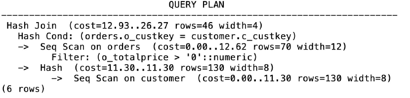
Figure 1. A qep in PostgreSQL.

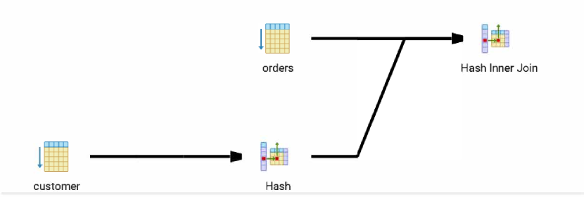
Figure 2. Visual tree representation of the qep.

Example 1.1.

Alice is an undergraduate cs student who is currently enrolled in a database course. She wishes to understand the execution steps of an sql query in PostgreSQL on a tpc-h benchmark dataset (tpch, ) by perusing the corresponding qep in Figure 1 (partial view). Unfortunately, Alice finds it difficult to mentally construct a narrative of the overall execution steps by simply perusing it. This problem is further aggravated in more complex sql queries. Hence, she switches to the visual tree representation of the qep as shown in Figure 2. Although relatively succinct, it simply depicts the sequence of operators used for processing the query, hiding additional details about the query execution (e.g., sequential scan, join conditions). In fact, Alice needs to manually delve into details associated with each node in the tree for further information.    

We advocate that an intuitive natural language-based description of a qep can greatly facilitate learners to comprehend how an sql query is executed by a rdbms. To support this hypothesis, we surveyed 62 unpaid volunteers taking the database course in an undergraduate cs degree program. We use the tpc-h v2.17.3 benchmark and a rule-based natural language generation tool for qeps  (neuron, ) to generate natural language (nl) descriptions of qeps for sql queries formulated by the volunteers (both ad hoc and benchmark queries). The volunteers were asked to select their most preferred qep format (i.e., json text, visual tree, and nl description) that aide in understanding the execution steps of these queries. Figure 3 depicts the results. Observe that nl description is the most preferred format. On the other hand, very few voted for the json format supported by PostgreSQL. Also, the visual tree representation of a qep has healthy support. Hence, we believe that an nl-based interface can effectively complement visual qeps to augment the learning experience of learners. Specifically, a learner may use the visual qep to get a quick overview of an execution plan and then peruse the nl description to acquire detailed understanding.

The majority of natural-language interfaces for rdbms (LJ14a, ; LJ14b, ; SF+16, ; KV+12, ), however, have focused either on translating natural language sentences to sql queries or narrating sql queries in a natural language. Scant attention has been paid for generating natural language descriptions of qeps. Natural language generation for qeps is challenging from several fronts. First, although deep learning techniques, which can learn task-specific representation of input data, are particularly effective for natural language processing, it has a major upfront cost. These techniques need massive training sets of labeled examples to learn from. Such training sets in our context are prohibitively expensive to create as they demand database experts to translate thousands of qeps of a wide variety of sql queries. Even labeling using crowdsourcing is challenging as accurate natural language descriptions demand experts who understand qeps. Note that accuracy is critical here as low quality translation may adversely impact individuals’ learning. Second, ideally we would like to generate natural language descriptions of qeps using one application-specific dataset (e.g., movies) and then use it for other applications (e.g., hospital). That is, the natural language generation framework should be generalizable. This will significantly reduce the cost of its deployment in different learning institutes and environments where different application-specific examples may be used to teach database systems.

In this paper, we present a novel end-to-end system called lantern (naturaL lANguage descripTion of quERy plaNs) to generate natural-language descriptions of qeps. Given an sql query and its qep, it automatically generates a natural language description of the key steps undertaken by the underlying rdbms to execute the query. To this end, instead of mapping an entire qep to its natural language description, we focus on mapping the set of physical operators in a rdbms to corresponding natural language descriptions and then stitch them together to generate the description of a specific qep. The rationale behind this strategy is as follows. Any rdbms implements a small number of physical operators to execute any sql query. Hence, although there can be numerous qeps, they are all built from a small set of physical operators. Consequently, it is more manageable to label these operators and generate the natural language description of any qep from them. This also allows us to generalize lantern to handle any application-specific database as the relations, attributes, and predicates can simply be used as placeholders in describing a physical operator. Lastly, it makes our framework orthogonal to the complexities of sql queries as they are all executed by a small set of physical operators.

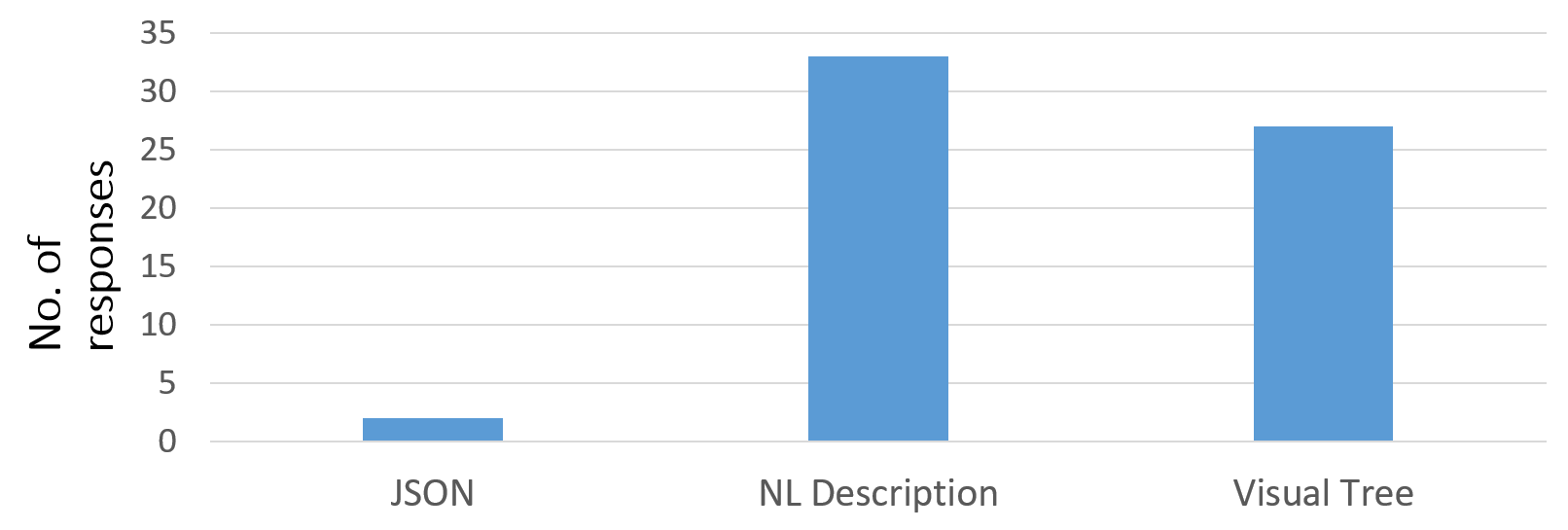
Figure 3. Survey of qep formats.

We present a flexible declarative framework called pool for succinctly specifying natural language descriptions of physical operators in an rdbms. We then develop a rule-based framework called rule-lantern to generate a natural language description of a qep by leveraging the specified descriptions of physical operators. We observe from our engagements with learners that although rule-based approach have high accuracy, it makes the descriptions of qeps monotonous leading to boredom. In fact, this is consistent with psychology theories that repetition of messages can lead to annoyance and boredom (CP79, ) (detailed in Section 6.1). To address this issue, we develop a novel deep learning-based language generation framework called neural-lantern that infuses language variability in the generated description by exploiting a group of paraphrasing tools (synonymous1, ; synonymous2, ; synonymous3, ) and pretrained word embeddings (devlin2018bert, ; mikolov2013efficient, ; pennington2014glove, ; ELMO, ). Importantly, it addresses the challenge of training data generation by first generating a large number of random queries based on schema information and actual values in the database and then utilize rule-lantern and the paraphrasing tools to generate a large number of natural language descriptions of the physical operators. We built lantern on top of PostgreSQL and SQL Server. Our exhaustive experimental study with real learners demonstrates the superiority of lantern to existing qep formats of commercial rdbms.

In summary, this paper makes the following contributions:

• We present a novel end-to-end system called lantern for generating natural language descriptions of qeps. It takes a concrete step towards the vision of natural language interaction with the relational query optimizer.

• We present a declarative framework called pool to enable subject matter experts (smes) to label physical operators in an intuitive way (Section 4).

• Based on the specifications using pool, in Section 5 we present a rule-based approach called rule-lantern to generate a natural language description of a qep.

• We present a novel psychology-inspired neural framework for natural language generation called neural-lantern in Section 6 that addresses limitations of rule-lantern. (e) In Section 7, we undertake an exhaustive performance study using synthetic and real-world datasets to demonstrate the effectiveness of lantern.

2. Related Work

Natural language interfaces to databases have been studied for several decades. Such interfaces enable users easy access to data, without the need to learn a complex query languages, such as sql. Specifically, there have been natural language interfaces for relational databases (ASB19, ), xml (LC+07, ), and graph-structured data (ZC+17, ). Given a logically complex English language sentence as query input, the goal of majority of these work is to translate it to the underlying query language such as sql (BJL19, ; BH+18, ; SF+16, ; Yl+16, ; YZ+18, ; YZ+19, ; BJ+20, ; WU19, ; ZXS, ; XC+19, ; KS+20, ). Recently, deep learning techniques have been utilized to translate natural language queries to sql (BH+18, ; UW+18, ; XC+19, ; Yl+16, ; YZ+18, ; YZ+19, ; ZXS, ). On the other hand, frameworks such as Logos (KV+12, ) explain sql queries to users using natural language. lantern compliments these efforts by providing a natural language description of a qep.

Most germane to this work is the demonstration of a system called neuron in (neuron, ), which generates natural language descriptions of qeps using a rule-based technique. It also supports a natural language question answering system that allows a user to seek answers to a variety of concepts and features associated with a qep. In contrast, we focus on generating a natural language description of a qep and give detailed methodology to address this problem. We also introduce a declarative framework for label specification and a deep learning-based solution that are omitted in (neuron, ). Finally, user studies and experiments demonstrating the effectiveness of the proposed frameworks are presented in this work.

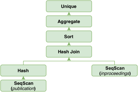
Figure 4. A physical operator tree (i.e., qep).

3. Preliminaries

In this section, we present basic concepts that are necessary to comprehend this paper.

Physical Operator Tree. The relational query execution engine implements a set of physical operators (SC98, ). An operator takes as input one or more data streams and produces an output data stream. Some examples of physical operators are sequential scan, index scan, and hash join. Note that in database literature, we typically refer to such operators as physical operators since there is not necessarily one-to-one mapping with relational operators. These physical operators are the building blocks for the execution of sql queries. An abstract representation of such an execution is a physical operator tree (operator tree for brevity), denoted as $T=(N,E)$, where $N$ is a set of nodes representing the operators and $E$ is a set of edges representing data flow among the physical operators. The physical operator tree is the abstract representation of a query execution plan (qep) and we use these terms interchangeably. The query execution engine is responsible for the execution of the qep to generate results of a sql query.

Example 3.1.

Consider the following sql query on dblp dataset.

SELECT DISTINCT(I.proceeding_key)
FROM inproceedings I, publication P
WHERE (I.proceeding_key = P.pub_key AND
       P.title like ’%July%’)
GROUP BY I.proceeding_key
HAVING COUNT (*) > 200;

The qep (i.e., physical operator tree) of the query generated by PostgreSQL is depicted in Figure 4.    

Intuitively, we classify the nodes in an operator tree of a qep into two categories, namely critical and auxiliary operators (nodes). The former type of nodes corresponds to important operations (e.g., HASH JOIN, SEQSCAN) in a qep. On the other hand, the latter type is located near a critical node (e.g., parent, child) and supports the execution of the operator represented by a critical node. For instance, HASH JOIN and HASH in Figure 4 are examples of critical and auxiliary nodes/operators in PostgreSQL, respectively .

Seq2Seq Model. The Seq2Seq model has revolutionized the process of machine translation using the deep learning framework (sutskever2014sequence, ). It has also been a standard method for other text generation applications such as image captioning (Vinyals-caption, ; Karpathy-image-cap, ), conversational models (Vinyals-dialog, ), text summarization (see-summ, ). The Seq2Seq model puts two neural networks together, one as an encoder and the other as a decoder. It takes as input a sequence of words and generates an output sequence of words. Given a source (input) sequence of words, the encoder-decoder framework works as follows. The encoder deep neural network converts the input words to its corresponding hidden vectors, where each vector gives a contextual representation of the corresponding word. The decoder deep neural network is a language model that takes as input the hidden vector generated by the encoder, its own hidden (previous) states and the current word to produce the next hidden vector and to finally predict the next word.

The encoder and the decoder can use a recurrent neural network (rnn) architecture (sutskever2014sequence, ) with carefully designed cells like lstm or gru, convolutional (convseq2seq, ; Wu-dynconv, ) or recently proposed transformer architecture (Vaswani-transformer, ). It is also common to employ an attention mechanism (Bahdanau-attn, ; luong2015effective, ) so that the decoder can selectively focus on relevant encoder states while generating a token.

4. A Declarative Framework

Ideally, we would like to have access to large volumes of labels that associate qeps to their corresponding natural language descriptions. Then, in principle, we can use such labels as training data to build a deep learning-based model to generate a natural language description of any qep. Unfortunately, although there is increasing availability of sql-to-natural language training datasets (YZ+18, ), to the best of our knowledge, no publicly-available data source exists for qeps. Note that natural language translation techniques for sql queries cannot be adopted here as sql queries are declarative and specified using logical operators. To further aggravate this issue, the natural language labeling of qeps needs to be performed by trained subject matter experts (sme) in order to ensure accuracy of the annotations. Given that there can be numerous qeps in practice, it is prohibitively expensive to deploy such experts for labeling qeps. On the other hand, crowdsourcing for cheaper sources of labeling is not a viable option as non-smes may not have sufficient background on query processing to annotate qeps with high degree of accuracy.

To address these challenges, we deploy smes to provide natural language descriptions for physical operators in a commercial rdbms in lieu of qeps. All qeps are essentially constructed from this set of operators, which is orders of magnitude smaller than a training set containing qeps, making natural language descriptions (i.e., labels) economical to obtain from smes. In order to expedite the labeling process, we propose a declarative framework where a sme can create and manipulate the labels using a declarative language called pool (Physical Operator Object Language). In this section, we elaborate on this framework. Note that we focus on features that are necessary to understand our rule-lantern framework.

4.1. Requirements

Investigation of physical operators in commercial rdbms as well as our engagement with learners identified several crucial requirements for pool. First, an abstract data type for physical operators is necessary so that smes may treat such data at a level independent from a specific rdbms.

Second, smes must be able to select objects to be labeled and specify corresponding natural language labels. In particular, they must be able to label physical operators in three dimensions, namely, create meaningful alias of a physical operator, natural language definition of an operator, and natural language descriptions of the operation performed by an operator. In particular, aliases are important as names of certain operators can be ambiguous to a learner. For instance, DB2 uses HSJOIN as the name of hash join operator. Hence, an alias of HASH JOIN is more intuitive to a learner. Similarly, a learner may encounter unfamiliar operators (e.g., zigzag join (ZZJOIN in DB2)) in her course. Hence, natural language definitions of such operators will be useful to her while perusing qeps.

Third, it may be necessary to declaratively combine labels of a pair of operators in order to generate a succinct natural language description of a qep. For instance, in PostgreSQL labels of HASH JOIN and HASH operators need to be combined to generate a natural language description of the former operator. An example of such description can be “hash $$R_{1}$$ and perform hash join on $$R_{2}$$ and $$R_{1}$$ on condition $$cond$$” where “hash $$R_{1}$$” is the label associated with the HASH operator.

Fourth, smes should be able to transfer the description of one operator to another to make specification of natural language descriptions of operators more efficient. For instance, hash join and nested-loop join are both join operators. Consequently, their descriptions may be very similar, i.e., the description of nested-loop join operator does not have the “hash $$R_{1}$$” segment. Hence, pool should be able to reuse and modify the existing description of hash join operator when specifying the description of nested-loop join operator. Similarly, one should be able to transfer the description or definition of hash join across different rdbms (e.g., PostgreSQL to DB2) without specifying it from scratch.

4.2. Features of POOL

Data Model. The data model underlying pool is called poem (Physical Operator ObjEct Model). poem is a simple and flexible graph model where all entities are objects. Each object represents a physical operator of a relational query engine. Each object has a unique object identifier ($oid$) from the type oid. Objects are either atomic or complex. Atomic objects do not have any outgoing edges. All objects have a set of attribute-value pairs. Specifically, each object is associated with the following attributes: source, name, alias, defn, desc, type, cond, and target. The source refers to the specific relational engine that an operator belongs to. The name refers to the name of a physical operator in the source and the type captures whether it is an unary or binary operator. Alias is an optional alternative name for an operator. The defn attribute stores the definition of an operator. The desc attribute stores a natural language description of the operation performed by an operator. The cond attribute takes a Boolean value to indicate whether a specified condition (e.g., join condition) should be appended to the natural language description of an operator. Values of all attributes are taken from the atomic type string (possibly empty). As an example, consider the HASHJOIN operator in PostgreSQL. In poem, it is an object with the following attributes: source = ‘postgresql’, name = ‘hashjoin’, alias = ‘ ’, type = ‘binary’, defn = ‘a type of join algorithm that uses hashing to create subsets of tuples’, desc = ‘perform hash join’, and cond = ‘true’. Note that the source serves as an entry point to the database. The set of objects is referred to as poem store.

There is a directed edge between an object pair ($p_{a}$, $p_{c}$) iff $p_{a}$ is an auxiliary operator and $p_{c}$ is a critical operator (recall from Section 3) in a qep in source. It is captured by the target attribute of $p_{a}$. For example, ($p_{\textsf{hash}}$, $p_{\textsf{hashjoin}}$) of PostgreSQL has a directed link. Hence, the target attribute value of $p_{\textsf{hash}}$ is ‘hashjoin’.

Data Definition. The data definition in pool allows one to declaratively create physical operator objects associated with a specific rdbms. The general format of the statement is as follows: CREATE POPERATOR ¡name¿ FOR ¡source¿ (¡attribute-value pairs¿). An example is as follows.

CREATE POPERATOR hashjoin FOR pg
(ALIAS = null,
TYPE = ’binary’,
DEFN = null,
DESC = ’perform hash join’,
COND = ’true’,
TARGET = null)

Note that name must exists in the set of physical operators supported by the specified rdbms engine (i.e., source). For instance, hashjoin is a physical operator in PostgreSQL (i.e., pg). The optional ALIAS attribute specifies an alternative name of the operator. For example, the operator ZZJOIN in DB2 can be given an alias ‘zigzag join’ . In the case an alias is unspecified, it can be either set to null or simply omitted from the definition. The TYPE is a mandatory attribute that can take either ‘unary’ or ‘binary’ value. The DESC attribute is mandatory, which allows one to specify a natural language description of the operation performed by the operator. Note that pool does not prevent one from describing several descriptions for a single operator. For instance, DESC = ‘execute hash join’ can be added to the above definition. Observe that no relation or condition is specified in DESC. This is because these are added automatically to DESC by exploiting TYPE and COND attributes of an operator. For instance, since TYPE = ‘binary’ in the above definition, two variables representing join relations will be added automatically to the description of hashjoin. Lastly, the TARGET attribute allows one to specify auxiliary-critical operator pair. If its value is non-empty, it must be an existing name in the source.

Data Manipulation. The key goals of the data manipulation component of pool are to provide syntactical means to support (a) retrieval of specific properties (i.e., attributes) of physical operators, (b) generation of the template for natural language description of an operator that can be subsequently used in a qep, and (c) update properties of physical operator objects. We elaborate on them in turn.

Retrieval of specific properties of physical operators follows sql-like SELECT-FROM-WHERE syntax. The SELECT-FROM clauses are mandatory for any retrieval task. Predicates in the WHERE clause are formulated upon attributes of poem objects. Every query result is a set of poem objects with specific attributes specified in the SELECT clause and satisfies the conditions in the WHERE clause. The following example shows the retrieval of the ZZJOIN operator object with defn attribute.

SELECT defn FROM pg WHERE name = ’zzjoin’

The following example shows retrieval of all objects representing the join operation in the source.

SELECT * FROM pg WHERE name LIKE ’%join’

Our framework also supports join queries especially between physical objects from multiple dbms.

pool supports a COMPOSE clause to specify generation of a natural language description template of an operator. Specifically, the COMPOSE clause uses the desc, type, and cond attributes of operators to generate the template. For example, the template generation for the HASH operator can be specified as follows.

COMPOSE hash FROM pg

The above state will return the template “hash $$R_{1}$$”, which can be subsequently used by our framework to generate specific description of the HASH operator in a qep. Note that the COMPOSE operator returns a value of type string instead of a poem object. Also, observe that $R_{1}$ is appended based on the type attribute of the hash object.

As mentioned above, pool allows composing a pair of critical and auxiliary operators (e.g., hash and hash join) to generate the natural language description template for the critical operator.

COMPOSE hash, hashjoin FROM pg
USING hashjoin.desc = ’perform hash join’

The above statement generates the following template: “hash $$R_{1}$$ and perform hash join on $$R_{2}$$ and $$R_{1}$$ on condition $$cond$$”. Since an operator object may have multiple desc attributes, the optional USING clause allows one to specify which one to use to generate the template. In the case it is unspecified, a desc will be chosen randomly for each operator in the COMPOSE clause to create the template. Hence, the form of a COMPOSE statement is: COMPOSE ¡list of object names¿ FROM ¡source¿ USING ¡condition on desc¿. Note that in the case the list of object names contains more than one operators, it must be an (auxiliary, critical) operator pair, which generates the template for the critical operator.

pool supports update statements that allow attributes of existing poem objects to be changed. The general form of the update statement is: UPDATE ¡source¿ SET ¡new-value assignments¿ WHERE ¡condition¿. Each new-value assignment is an attribute, an equal sign and a string. If there are more than one assignment, they are separated by commas. The following example shows updating the definition of the hash join operator.

UPDATE pg
SET defn = ’a type of join algorithm...’
WHERE name = ’hashjoin’

The update statement can be exploited to assign definition or description of an operator from one commercial database to another, thereby making it more efficient for an sme to specify properties of physical operators. The following example demonstrates how description of hash join in PostgreSQL is transferred to the hash join operator in DB2.

UPDATE db2
SET desc = (SELECT desc
 FROM pg WHERE pg.name = ’hashjoin’)
WHERE db2.name = ’hsjoin’

It can also be used along with the REPLACE clause to transfer definition or description of an operator to another within the same source. For example, one can transfer the description of hash join to nested loop join by replacing the word ‘hash’ with ‘nested loop’ as follows.

UPDATE pg
SET desc = REPLACE((SELECT desc FROM pg AS pg2
WHERE pg2.name = ’hashjoin’), ’hash’, ’nested loop’)
WHERE pg.name = ’nested loop join’

Note that the REPLACE clause takes three parameters as input, namely the description or definition of a poem object, the string in it that needs to be replaced (e.g., ‘hash’), and its new replacement string (e.g., ‘nested loop’).

Implementation. pool is implemented on top of a standard relational database. poem objects are stored in two relations with the following schema: POperators(oid, source, name, alias, type, defn, cond, targetid) and PDesc(oid, desc) as an object may have multiple descriptions. We use Python script to translate pool statements to corresponding sql statements on these relations. A wrapper is implemented that takes the results of sql queries as input and returns poem objects or string as output.

5. The Framework of Rule-LANTERN

Our rule-based framework, rule-lantern, leverages the narration (descriptions by smes) of various operators defined using pool to generate a natural language description of the qep of an sql query. In this section, we describe it in detail. We begin with the model of the framework for generating natural language descriptions of qeps. Next, we highlight the key issues for designing rule-lantern. Finally, we present the algorithm for realizing rule-lantern.

5.1. Model For Narration of QEPs

Narration is the use of techniques to convey a story to an audience (narration, ). In our context, the story is the description of a query execution plan and the audience consists of learners. Chatman (Chatman, ) defines narrative as a story (content of the narrative) and discourse (expression of it). In a nutshell, the story can be viewed as the logical form of the narrative, while the discourse prunes out unimportant content and focuses on presenting components deemed interesting in a particular order.

Inspired by this classical model of narration, El Outa et al. (OF+20, ) recently proposed a four-layered model for data narration that we adopt for qeps. Specifically, the narration of qeps is modeled as follows.

• Factual layer. The factual layer models qeps (i.e., data) using language-annotated operator trees that allow for manipulation of qeps for narration generation.

• Intentional layer. The intentional layer models the substance of a story by identifying the content (description of various operators) based on the desired goal (i.e., comprehension of a qep by learners).

• Structural layer. The structural layer models the structure of a narrative by organizing its plot (i.e., the arrangement of messages in a way easily understandable by the audience). While the previous layers focus on the contents of the narrative, this layer focuses on its discourse. In our framework, we organize the plot as a sequence of steps.

• Presentation layer. It models the presentation of a narrative. That is, how a story is presented to the audience.

Our rule-lantern addresses the first three layers. We utilize the presentation approach of (neuron, ) for the presentation layer.

5.2. Design Issues

At first glance, we may simply perform a post-order traversal of an operator tree and exploit the natural language description templates specified using pool to transform the information contained in each node “independently” to its natural language description and simply aggregate them to generate the description of a qep. This method, however, may produce a verbose description containing redundant information. This is because a node in an operator tree may only convey a segment of information related to a specific physical operator. For instance, in PostgreSQL, the node representing HASH JOIN have a child called HASH. The latter node conveys the hashed relation and can be considered as a part of the main narrative of performing hash join between two relations. Hence, it is important to consider the roles played by different nodes for generating concise natural language descriptions of qeps.

A consequence of the above issue is that the natural language description of an execution step related to a specific operation may need to be generated by composing descriptions of multiple nodes. For example, consider the TBSCAN operator (i.e., table scan operator in DB2). In one qep, we may simply perform a table scan on a relation without any filtering condition. On the other hand, in another qep, we may perform a table scan on a relation based on certain filtering condition (e.g., title contains ‘July’) using the FILTER operator. Hence, in the former plan, the natural language description is simply based on the TBSCAN node whereas in the latter plan, concise description demands composition of desc attributes of TBSCAN and FILTER nodes. Hence, rule-lantern should support such composition.

5.3. Language-annotated Operator Tree

Observe that an operator tree does not contain any information related to natural language descriptions of the operators. Hence, we extend it to annotate the nodes with their natural language descriptions as specified using pool. We refer to such extension as language-annotated operator tree (lot), denoted as $T_{L}=(N,E)$. Formally, each node $n\in N$ in $T_{L}$ is associated with a name, denoted as $n.name$, and a label, denoted as $n.label$. The former is set to the alias value of the corresponding object in poem. In the case the alias is unspecified, it is set to the object’s name. The latter contains a natural language description of $n$ generated from the natural language template created by executing COMPOSE statement of pool on $n$. For example, reconsider the operator tree in Figure 4. For the node representing hash join, $n.name=\textsf{HASH JOIN}$. A natural language description of this node can be $n.label=$ “perform hash join on table $$R_{1}$$ and table $$R_{2}$$ on condition $$C$$” where $R_{1}$ (resp. $R_{2}$) and $C$ are place holders for input relations and join condition(s), respectively. Note that this template is returned by the following pool query: COMPOSE hashjoin FROM pg. Also, specific relation/attribute names and conditions to replace the placeholders are added in subsequent steps.

5.4. Composition of Node Labels

To tackle the issues described in Section 5.2, we logically refine a lot by clustering the auxiliary nodes with the corresponding critical ones. Recall that these two types of nodes are specified by an sme using pool. For example, in PostgreSQL, HASH JOIN node and its child HASH, MERGE JOIN node and its child SORT are two examples of auxiliary-critical node pairs that can be specified using pool.

Given a lot $T_{N}=(N,E)$, $cluster(T_{N})$ returns a set pairs of nodes in $T_{N}$, $\{(n_{a},n_{c})|(n_{a},n_{c})\in E\wedge n_{a}\neq n_{c}\}$, where $n_{c}$ and $n_{a}$ denote critical and auxiliary nodes, respectively. Each pair of critical and auxiliary nodes in a cluster is translated into a single natural language description template using the COMPOSE statement as an auxiliary node contributes to a segment in the description. For example, consider the HASH JOIN and its child HASH in a lot. A natural language description template of this pair of nodes can be as follows: “hash $$R_{1}$$ and perform hash join on $$R_{2}$$ and $$R_{1}$$ on condition $$cond$$”. Observe that the segment “hash $$R_{1}$$” is generated from the HASH node.

Under the hood, the COMPOSE statement on a pair of nodes is realized using a composition operator, denoted by $\circ$. Given a pair of critical and auxiliary nodes $(n_{a},n_{c})$ such that $(n_{a},n_{c})\in E$, $n_{a}\circ n_{c}=n_{a}.label\wedge n_{c}.label$ where $\wedge$ represents “and’’. In the above example, $n_{a}.label=$ “hash $$R_{1}$$” and $n_{c}.label=$ “perform hash join on $$R_{2}$$ and $$R_{1}$$ on condition $$cond$$”. The composition operator is neither associative nor commutative. The left operand must be an auxiliary node. This is intuitive as the natural language description is unclear if “hash $$R_{1}$$” appears after the label of HASH JOIN.

5.5. Algorithm

Algorithm 1 outlines the procedure for generating a natural language description of a qep in rule-lantern. It first extends the operator tree $T$ to a lot $T_{L}$ (Line 1). Observe that in a graphical representation of a qep (e.g., Figure 2), hierarchical relations between operators and data flow are clearly indicated by edges in the tree. In contrast, a natural language description is inherently sequential as a reader reads it top-down like a document. Particularly, a parent of an operator may not be translated immediately as the next step during natural language generation as other children need to be translated first (e.g., auxiliary nodes). Therefore, in order to ensure clarity of data flow, this step also assigns a unique identifier to the output of each operator (i.e., intermediate results) so that it can be appropriately referred to in the translation of its parent (denoted by $node.identifier$). For example, in Figure 4, the intermediate results of the SEQSCAN operation on the Publication relation is assigned an identifier $T_{1}$. This identifier is subsequently used in the natural language description of its parent HASH node.

Next, it retrieves the cluster $C$ in $T_{L}$ containing a set of critical and auxiliary node pairs by leveraging the poem store (Line 2). Since the structural layer of our model consists of a sequence of steps to describe the qep, it traverses $T_{L}$ in post-order manner to generate these steps. If a node and its child are an element in $C$ then it uses the label of the critical node to generate corresponding natural language description by replacing the place holders with corresponding values (Lines 5-6). For example, in Figure 4, the HASHJOIN node satisfies the condition in Line 5 and is translated as follows: “hash $T_{1}$ and perform hash join on inproceedings and $T_{1}$ on condition ((i.proceeding_key)= (p.pub_key))”. Observe that $T_{1}$ is the identifier of intermediate results of the SEQSCAN node. On the other hand, if a node is not in $C$, then the corresponding $step$ is generated by utilizing its label. For example, the right leaf node is translated to “perform sequential scan on inproceedings”. Finally, the intermediate relation information is appended to $step$ in Lines 10-11. For instance, the segment “to get the intermediate relation $T_{2}$” is appended to the above $step$ of the HASHJOIN node. In the case, the node represents the final operation in an operator tree, “to get the final results.” is appended to $step$ (Line 13). Observe that contents of these nodes represent the intentional layer of our model. The time complexity of generating a natural language description is $O(N)$.

Algorithm 1 rule-lantern Algorithm

Input: An operator tree $T=(N,E)$, poem store $P$;
Output: Natural language translation $result$;

1:  $T_{L}\leftarrow$ GenerateLOT($T,P$)

2:  $C\leftarrow$ Cluster($T_{L}$, $P$)

3:  for all $node\in T_{L}$ do

4:     $step\leftarrow\emptyset$

5:     if $(node.child,node)\in C$ then

6:        $step\leftarrow$ Translate($node.child,node,step$)

7:     else

8:        $step\leftarrow$ Translate($node.label,step$)

9:     end if

10:     if $node.parent!=\emptyset$ and $node.identifier!=\emptyset$ then

11:        $step\leftarrow$ AppendIntermediate($step$, $node.identifier$)

12:     else if $node.parent=\emptyset$ then

13:        $step\leftarrow$ AppendFinal($step$, “to get the final results.’’ )

14:     end if

15:     $result\leftarrow$ Add($result$, $step$)

16:  end for

17:  return  $result$

Example 5.1.

Consider the operator tree in Example 3.1. The rule-lantern algorithm generates the description of the qep as the following sequence of steps. (1) Visit SEQ SCAN for table inproceedings and generate “perform sequential scan on inproceedings.” (Line 8). Note that the $identifier$ of intermediate results associated with this node is set to null as there is no filtering condition (i.e., intermediate relation is identical to the base relation). (2) Visit SEQ SCAN for table publication and generate “perform sequential scan on publication and filtering on (title containing ’July’) to get the intermediate relation $T_{1}$.” (Lines 8, 11). (3) Visit HASH JOIN and generate “hash table $T_{1}$ and perform hash join on inproceedings and $T_{1}$ on condition ((i.proceeding_key)= (p.pub_key)) to get the intermediate relation $T_{2}$.” (Lines 6, 11). (4) Visit AGGREGATE and generate “sort $T_{2}$ and perform aggregate on $T_{2}$ with grouping on attribute i.proceeding_key and filtering on (count(all) ¿ 200) to get the intermediate relation $T_{3}$.” (Lines 6, 11). (5) Visit UNIQUE and generate “perform duplicate removal on $T_{3}$ to get the final results.” (Lines 8, 13).    

Remark. It is worth noting that the aforementioned algorithm is generic and can be realized on any commercial rdbms. Specifically, although the physical operator names are different across different rdbms, the rule-lantern framework operates on $T_{L}$ and $C$, which are generated using the poem store.

6. Neural-LANTERN Framework

Although the rule-lantern technique can generate accurate natural language descriptions of qeps, our engagement with learners revealed an intriguing problem of this approach. Since the natural language description of an operation is generated from sme-specified descriptions in the poem store, the descriptions in qeps can be repetitive and lack variability. For example, the description in Step 3 of Example 5.1 will be repeated for all qeps containing a hash join operator although the input relations or join conditions may differ. Note that even though pool allows an sme to specify multiple descriptions of an operator, in practice she may only specify one. Consequently, some learners found that after reading the descriptions for several queries, they feel bored due to the usage of the same language to describe the operations. They reported that they started skipping several sentences in the descriptions. In fact, this is consistent with research in psychology that have found that repetition of text messages can lead to annoyance and boredom (CP79, ) resulting in purposeful avoidance (HK13, ), content blindness (HG+11, ), and even lower motivation (SPC90, ). To mitigate this problem, we propose a novel neural network-based framework called neural-lantern that is inspired by theories from psychology.

6.1. Habituation and Boredom

In psychology theory, habituation is a decrease in response to a stimulus after repeated presentations (habituation, ). The advantage of habituation is that it enables individuals to tune out unimportant information to be more productive or efficient. However, it also creates boredom that makes an individual disinterested in the information. Specifically, many studies in psychology such as  (ohanlon81, ) reported that habituation of cortical arousal in response to repetitive stimulation contribute to the likelihood that boredom is experienced. In fact, subjectively monotonous activities could lead to a high degree of frustration and boredom (HP85, ). Simple and homogeneous stimulus (e.g., same or similar messages) as well as high exposure, accelerate the appearance of boredom (HC72, ).

Diverse messaging has been studied to mitigate the problems germinated from repeated exposure. In controlled experiments, diversification was shown to reduce tedium from repeated exposure (HC72, ; SPC90, ). However, the messages were manually developed in these studies. Recall that pool also allows specifying such manual description using multiple desc attribute values. However, such manual generation creates a major barrier for diversifying descriptions of operators in qeps. Hence, systematic and automated technique is necessary for mitigating the negative effects of repeated exposure of similar descriptions.

6.2. Training Data Generation

If we regard a qep as an input language while the natural language description as the output, interpreting qep into natural language can be viewed as a machine translation task, which can be addressed by a deep learning-based framework. However, as remarked earlier, it brings in two key challenges. First, it is prohibitively expensive to get large volumes of training data for this task. Second, the description generated as output should mitigate the appearance of boredom among learners when they peruse the natural language descriptions of qeps. We address these challenges by presenting a neural network-based framework called neural-lantern. We begin with the training data generation process in this framework.

The training sample of a translation task consists of two parts, the sentence in the original (resp., input) language to be translated, i.e., the input operator tree, as well as the ground-truth translation in the output language, i.e., the natural language description of the corresponding qep. We shall now discuss these parts in turn.

Input. Given a relational database, we need a large number of sql statements in order to generate a large number of corresponding qeps for translation. Hence, we adopt the approach in (DBLP:conf/cidr/KipfKRLBK19, ) to generate a set of sql queries given a particular schema and database instance. This enables us to generate thousands of queries given a relational database instance. These queries contain aggregation, projection, as well as various filtering and join predicates.

Next, we acquire a collection of qeps corresponding to these queries. Each qep is decomposed into a set of acts (denoted as $actCol$), each of which corresponds to a set of operators over some relations. For instance, in Figure 4, SEQUENTIAL SCAN and (HASH JOIN, HASH) are two acts. Specifically, each act is a single node (i.e., operator) or a cluster (recall from Section 5.4) in an operator tree. Each of such act, in the form of some operators and corresponding relations/conditions, is employed as an input training sample, and its corresponding natural language description is used as output sequence in the translation model. Specifically, for each act, we employ the strategy in rule-lantern to generate the corresponding lot in order to generate its corresponding natural language description. Observe that our input is at the act-level (i.e., a subtree of an operator tree) instead of the entire operator tree. This enables us to not only generate numerous training data at specific operator-level but also, as we shall see in the next subsection, facilitates injecting diversity in the natural language description of each act, which in turn improves the neural model generalization.

Output. For each training act, we have to obtain its natural language translation as the output sequence. We apply rule-lantern to generate the natural language description for each input. Notably, we need to pay attention to the schema-dependent variables, e.g., relation/column names and filtering conditions, which do not contribute to the training of a translation model. We mark them with special symbols in the output labels for each input operation. For example, an INDEX SCAN node is translated by rule-lantern into the followings: “perform index scan on $$R_{1}$$ and filtering on $$C$$ to get the intermediate relation $$R_{2}$$”. We replace it with “perform index scan on $<$T$>$ and filtering on $<$F$>$ to get the intermediate relation $<$TN$>$” in the output label. Herein, special tags are adopted in the output to replace specific relations or predicates. The set of special tags we use is shown in Table 1. This leads us to a set of training samples, each of which consists of an operation (i.e., act) as input and a corresponding nl description as output.

Table 1. List of special tags used in the output.

Tag	Description	Example
$<$I$>$	indexed column name
$<$F$>$	filtering condition	$c\_mktsegment$ = ’BUILDING’
$<$C$>$	join condition	$c\_custkey=o\_custkey$
$<$T$>$	an existing temporary table name
$<$TN$>$	new temporary table name
$<$A$>$	column name for sort	order by revenue desc …
$<$G$>$	column name for groupby	group by $l\_orderkey$ …

6.3. Diversifying Translation

The preceding subsection describes a strategy to generate training data automatically instead of manual labeling. Specifically, the output labels for the training samples are all generated by rule-lantern. Consequently, it does not address two key challenges discussed earlier. First, the translation generated by rule-lantern can be repetitive leading to possible boredom among learners while reading the natural language descriptions of qeps. Second, the amount of training data generated is still limited since rule-lantern imposes a one-to-one mapping between an act and its corresponding natural language description.

To address these challenges, we employ three popular state-of-the-art synonymous sentence generation tools (synonymous1, ; synonymous2, ; synonymous3, ) to expand the training samples as well as inject diversity in the translated text. For the same sql statement, these models can generate a variety of natural language descriptions that add diversity to the narrative. In particular, for each of the rule-lantern results, we apply all the three tools and acquire a set of synonymous sentences. Notably, we remove duplicates (if any) and manually eliminate invalid sentences generated by these tools. As a result, we enlarge the number of training samples in our datasets by approximately 3 times.

Table 2 shows an example of three synonymous sentences generated by these tools from a rule-lantern-generated text. An interesting observation is that these tools may not always choose correct words in the generated sentences. For example, in sentences 1 and 2, the word “separating” is generated instead of “selecting”. At first glance, it may seem that this may hinder a learner’s comprehension. However, surprisingly, our empirical study shows that is not the case. Instead, it may even arouse interest among learners as they encounter novel unexpected words.

6.4. Translation Model

Task definition. To finish our translation task, we present a QEP2Seq model following the Seq2Seq structure. For a qep, the acts collection $actCol$ is composed of a series of acts ${L_{1},L_{2},\ldots,L_{n}}$, each of which is derived from the qep. Specifically, each act $L_{i}$ constitutes an input to the neural Seq2Seq model, and the corresponding output is the generated description $S_{i}$ containing $m$ tokens ${o_{1},o_{2},\ldots,o_{m}}$, with $o_{t}$ being the word at position $t$. Our goal is to train a model parameterized by $\theta$ that can be used to infer the most likely natural language description $S_{i}$ for any given input $L_{i}$ as follows:

(1) $$\hat{S}_{i}=\mathop{\arg\max}_{y_{{1:m}}}\prod_{t=1}^{m}P_{\theta}(y_{t}=o_{t}|y_{0:t-1},L_{i})$$

The explanation for the entire qep containing acts ${L_{1},L_{2},\ldots,L_{n}}$ is then constructed by concatenating the $\hat{S}_{i}$’s for $i=1\ldots n$.

Table 2. Examples of synonymous sentence generation.

Approach	Description
rule-lantern	perform sequential scan on user and filtering on age $>$ 10 to get the final results.
synonymous sentence 1	perform sequential scan on user and separating on age $>$ 10 to get the conclusive outcome.
synonymous sentence 2	execute sequential scan on user and separating on age $>$ 10 to get the conclusive outcome.
synonymous sentence 3	execute sequential scan output on user and get user which age $>$ 10 and to get the conclusive outcome.

6.4.1. Model Architecture

As shown in Figure 5, our QEP2Seq model consists of an Encoder and a Decoder. The decoder employs an attention mechanism so that it can focus on the relevant portion of the input when generating a target word. Besides, we also use pre-trained word vectors in the Decoder (see Embedding in Figure 5).

Pre-trained word vectors. Static and contextualized pre-trained word representations like GloVe (pennington2014glove, ), Word2Vec (mikolov2013efficient, ) and BERT (devlin2018bert, ) have attracted a great amount of attention recently in nlp. The vector representations of words learned by these models have been shown to carry semantic information that can help the model to generalize well for different nlp tasks.

In this work, we adopt both static (Word2Vec and GloVe) and contextual word embeddings (ELMo (elmo, ) and BERT). While static word embeddings are easy to use, using contextual embeddings effectively can be non-trivial. For ELMo, we take the embeddings from its two bi-lstm layers (each of size 4096) and take a linear combination of the vectors as the pre-trained representation of a word. For BERT, we take the representation from its last layer. We use the BERT-based model, which has 12 layers with 768 hidden units and 12 heads. Empirical study in the next section demonstrates that using pre-trained word embeddings can accelerate the convergence of our QEP2Seq model and alleviate overfitting problem.

Encoder. The Encoder rnn encodes each word $w_{t}$ in $L_{i}$ into the corresponding hidden state $\mathbf{h}_{t}$ using an lstm layer. The lstm maintains a vector of memory cells $\mathbf{c}_{t}\in\mathbb{R}^{d}$ (a.k.a. cell state) to store long term memory, and uses (soft) gates to control how much information to update with, to retrieve, or to remember for the next token. At each time step $t$, the lstm hidden layer receives previous hidden state $\mathbf{h}_{t-1}$ and the current input $\mathbf{x}_{t}$, i.e., the word embedding for token $w_{t}$ (randomly initialized). The $LSTM_{\text{Enc}}(\mathbf{h}_{t-1},\mathbf{x}_{t})$ architecture used here is given by the following equations (graves2013speech, ):

(2) $$\mathbf{i}_{t} = \mathrm{sigmoid}(U_{i}\mathbf{h}_{t-1}^{l}+V_{i}\mathbf{x}_{t})\hskip 40.00006pt\text{[input gate]}$$

(3) $$\mathbf{f}_{t} = \mathrm{sigmoid}(U_{f}\mathbf{h}_{t-1}^{l}+V_{f}\mathbf{x}_{t})\hskip 35.00005pt\text{[forget gate]}$$

(4) $$\mathbf{o}_{t} = \mathrm{sigmoid}(U_{o}\mathbf{h}_{t-1}^{l}+V_{o}\mathbf{x}_{t})\hskip 35.00005pt\text{[output gate]}$$

(5) $$\mathbf{c}_{t} = \mathbf{i}_{t}\odot\tanh(U_{c}\mathbf{h}_{t-1}^{l}+V_{c}\mathbf{x}_{t})+\mathbf{f}_{t}\odot\mathbf{c}_{t-1}\hskip 5.0pt\text{[cell state]}$$

(6) $$\mathbf{h}_{t} = \mathbf{o}_{t}\odot\tanh(\mathbf{c}_{t})\hskip 100.00015pt\text{[output]}$$

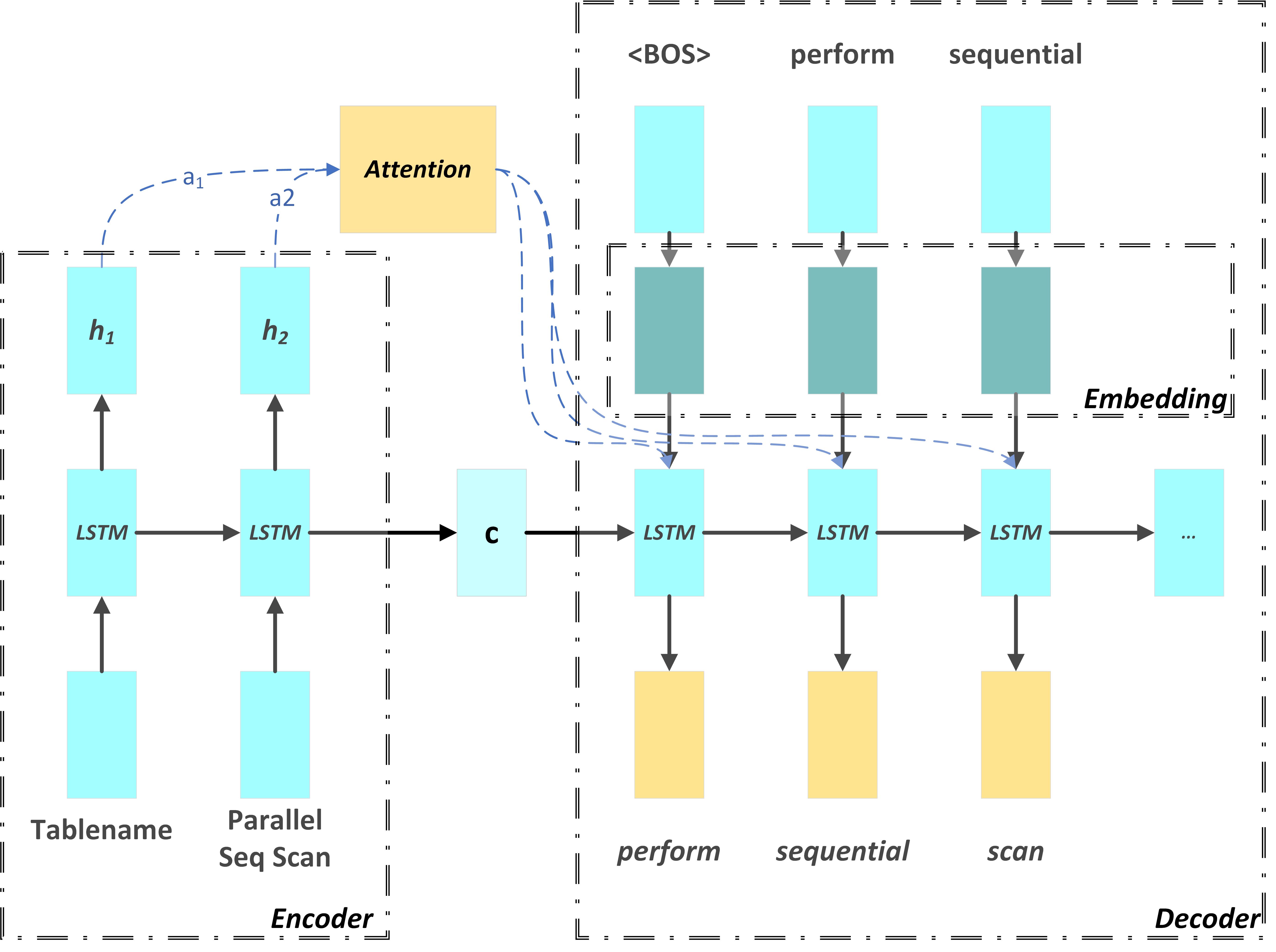
Figure 5. The QEP2Seq Model.

where $U_{\cdot}$ and $V_{\cdot}$ are the corresponding weight matrices and $\odot$ denotes element-wise product.

Decoder with attention. To generate the natural language description ($S_{i}$) for the input sequence ($L_{i}$), we use an lstm decoder with an attention mechanism (luong2015effective, ). The attention is an elegant way to let the decoder focus on the relevant portion of the encoder while generating a token (Figure 5). Similar to the Encoder rnn, at each time step $t$, the decoder rnn receives two inputs – the previous hidden state $\mathbf{s}_{t-1}$ and the word embedding $\mathbf{x}_{t}$ (e.g., Word2Vec, BERT). The lstm layer then constructs $\mathbf{s}_{t}$ following Equations 2 - 6 (using a different set of weight matrices).

(7) $$\mathbf{s}_{t}=LSTM_{\text{Dec}}(\mathbf{s}_{t-1},\mathbf{x}_{t})$$

The decoder hidden state $\mathbf{s}_{t}$ is then used to compute a relevance score (attention weight) with respect to each of the encoder states $\mathbf{h}_{t}\textsf{ for }t=1\ldots N$ with $N$ being the number of tokens in $L_{i}$ (Eq. 8).

(8) $$\alpha_{i}^{t}=\frac{\exp(g(\mathbf{s}_{t},\mathbf{h}_{i}))}{\sum_{j=1}^{N}\exp(g(\mathbf{s}_{t},\mathbf{h}_{j}))}$$

In particular, $g(\mathbf{s}_{t},\mathbf{h}_{i})$ is a relevant score between the hidden state $\mathbf{s}_{t}$ of the Decoder and the hidden state $\mathbf{h}_{i}$ of the Encoder. There are several ways to compute the relevant scores. In our work, we use the additive attention (Bahdanau-attn, ) to measure the relevance score:

(9) $$g(\mathbf{s}_{t},\mathbf{h}_{i})=V_{a}^{T}\tanh(W_{s}\mathbf{s}_{t}+W_{h}\mathbf{h}_{t})$$

where $V_{a},W_{s}$, and $W_{h}$ are learnable parameters. The attention weights are then used to compute a context vector $\mathbf{a}_{t}$ as a weighted sum of encoder hidden states (Eq. 10).

(10) $$\mathbf{a}_{t}=\sum_{i=1}^{N}\alpha_{i}^{t}\mathbf{h}_{i}$$

We concatenate the lstm state $\mathbf{h}_{t}$ and the context vector $\mathbf{a}_{t}$ and use the concatenated vector to compute the generation probability over the vocabulary items $o\in\mathcal{O}$ (Eq. 11).

(11) $$P_{\theta}(y_{t}=o|y_{0:t-1},L_{i})=\frac{\exp(\mathbf{w}_{o}^{T}[\mathbf{s}_{t};\mathbf{a}_{t}])}{\sum_{o^{\prime}\in\mathcal{O}}\exp(\mathbf{w}_{o^{\prime}}^{T}[\mathbf{s}_{t};\mathbf{a}_{t}])}$$

where $\mathbf{w}_{o}$ is the weight vector corresponding to the output word $o$.

6.4.2. Model Training

We minimize the cross entropy loss and use Teacher Forcing (williams1989teacherforcing, ) to train the Seq2Seq model. Teacher forcing, where current step’s target token is passed as the next input to the decoder rather than the predicted token, is a common way to train neural text generation models for faster convergence. The loss for one input-output pair $(L_{i},S_{i})$ can be written as:

(12) $$\mathcal{L}(\theta)=-\sum_{t=1}^{m}\sum_{o\in\mathcal{O}}\mathbbm{1}(y_{t}=o)\log P_{\theta}(y_{t}=o|y_{0:t-1},L_{i})$$

where $\mathbbm{1}(y_{t}=o)$ is an indicator function that returns $1$ if $y_{t}=o$ otherwise $0$. Our LSTM layer has 256 cells at each layer, with an input vocabulary of 36 and an output vocabulary of 62. The statistics about the word embeddings and the resulting LSTM parameters are listed in Table 3. The complete training details are given below:

Method	Dimension of embedding	#parameters (total)	#pure recurrent connections (Encoder, Decoder)
QEP2Seq+Word2Vec	128	920,393	837,632 (279,552, 558,080)
QEP2Seq+GloVe	100	993,901	907,264 (279,552, 627,712)
QEP2Seq+BERT	768	1,716,009	1,591,296 (279,552, 1,311,744)
QEP2Seq+ELMo	1024	1,992,745	1,853,440 (279,552, 1,573,888)

Table 3. Statistics about our LSTM layer.

• We initialized all of the lstm’s parameters with the uniform distribution between -0.1 and 0.1

• We used stochastic gradient descent (sgd) without momentum, with a fixed learning rate of 0.001. We trained our models for a total of 50 epochs.

• We used minibatches of 4 sequences.

• The dimension of the word embedding in the Encoder is 16, and at the Decoder is 32 when no pre-trained word vector is employed (i.e., for random initialization).

• We select our model based on the validation loss.

6.4.3. Natural Language Generation

After the QEP2Seq model is trained, the most likely description can be inferred (or decoded) by:

(13) $$\hat{S}_{i}=\mathop{\arg\max}_{y_{{1:m}}}\prod_{t=1}^{m}P_{\theta}(y_{t}|y_{0:t-1},L_{i})$$

In the above equation, $\theta$ denotes the trained QEP2Seq model, and $\prod_{t=1}^{m}P_{\theta}(y_{t}|y_{0:t-1},L_{i})$ is the probability that the model assigns to sequence $y_{{1:m}}$ for an input sequence $L_{i}$. In practice, the argmax procedure is intractable for large output vocabulary. To overcome that, we employ a Beam Search algorithm, which maintains a beam of $K$ partial hypothesis starting with the start symbol $<$BOS$>$ (as shown in Figure 5). At each step, the beam is extended by one additional character and only the top $K$ hypotheses are kept. Decoding continues until the stop symbol $<$END$>$ is emitted, at which point the hypothesis is added to the set of completed hypotheses.

Finally, we replace the special tags (e.g., $<I>,<C>,\ldots$) listed in Table 1 in the generated natural language using the corresponding identifiers.

Remark. The neural-lantern framework is novel in the following ways. First, this is a seminal effort to model the qep to natural language description as a machine translation task. Second, our training data generation process is designed to address the psychological impact of repeated text on learners. Third, we propose a novel QEP2Seq scheme. As a qep cannot be regarded as an input sequence, we present a model to interpret qeps into a set of acts, each of which is viewed as an input for the translation model.

7. Experimental Study

lantern is implemented in Python. In this section, we report the performance results of lantern. All experiments are performed on a server running Ubuntu 16.04.6 LTS with 2*Intel Xeon CPU E5-2680 v2 @ 2.80GHz, 256GB RAM, and 2*NVIDIA RTX 2080 Ti graphical card with 11GB GDDR6.

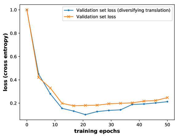
(a) Diversification of text

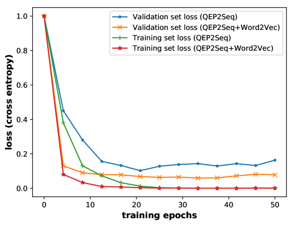
(b) Pre-trained word vectors

Figure 6. Paraphrasing and pre-trained word vectors.

7.1. Experimental Setup

Datasets. By default, we use PostgreSQL v10.12.2 as the underlying rdbms. Two smes used pool to generate the descriptions of all physical operators to create the poem store. We use the tpc-h benchmark (tpch, ), sdss (sdss, ), and imdb (imdb, ) datasets as representatives of application domains. In particular, a recent benchmarking study (KS+20, ) reported that existing nl2sql techniques perform poorly on tpc-h dataset containing complex and diverse sql queries.

We train our QEP2Seq model in neural-lantern using the workloads in tpc-h and sdss. For instance, given the 22 queries in tpc-h, we obtain their corresponding qeps. The qeps are then decomposed into 544 acts. For each of them, we generate a series of natural language descriptions following the procedure described in Section 6.2, resulting in 1632 samples. On the other hand, we generate 608 samples from the 71 predefined workload (http://skyserver.sdss.org/dr16/en/help/docs/realquery.aspx) in sdss. The neural network is implemented using Keras 2.2.4 and TensorFlow 1.13.2. We use Word2Vec (WV, ), GloVe (glove, ), ELMo (elmo, ), and BERT (bert, ) as pre-trained word vectors in the Decoder.

Note that sdss is tailored for SQL Server. Hence, we implement rule-lantern (neural-lantern relies on QEP2Seq and is orthogonal to the underlying rdbms) on SQL Server (v15.0) as follows. First, qeps of SQL Server are in xml format. Hence, we implement a parser to transform a qep to the corresponding operator tree. Second, all physical operators of SQL Server are created using pool and stored in the poem store. In summary, we can extend lantern to any rdbms easily by writing a parser to create operator trees and updating the poem store with rdbms-specific physical operators.

Finally, from all the samples, 80% of them are randomly selected to train the model, while the remaining 20% are selected as the validation set. Note that the performance of QEP2Seq is affected by the average number of training samples for each operator. In our experiments, there are on average 100 samples for each operator.

Method	Self-BLEU	#Samples per group
Without paraphrasing	1.0	1
paraphrasing with (synonymous3, )	0.309	2
paraphrasing with (synonymous2, )	0.603	2
paraphrasing with (synonymous1, )	0.502	2
paraphrasing with (synonymous1, ; synonymous2, ; synonymous3, )	0.482	4

Table 4. Diversity among the training samples.

The trained model is applied to imdb for testing to demonstrate the portability of lantern across different domains. Specifically, we generate 1000 sql queries using the approach in (DBLP:conf/cidr/KipfKRLBK19, ). The corresponding qeps for these queries are then decomposed into 5232 acts, each of which is viewed as a test sample.

Algorithms. We compare lantern with neuron (neuron, ), a rule-based approach for generating natural language descriptions of qeps. We also compare it with the textual and visual tree-based descriptions of qeps in PostgreSQL/SQL Server.

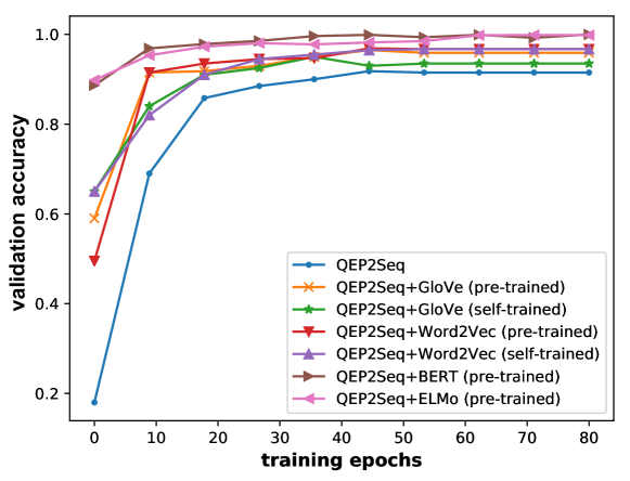
(a) pre-trained vs. self-trained

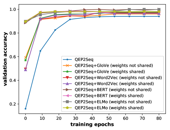
(b) w or w/o learned parameters

Figure 7. Impact of pre-trained vectors.

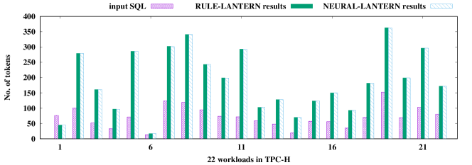
(a) Length of input vs. output.

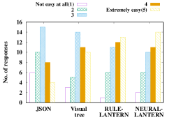
(b) Question Q1

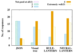
(c) Question Q2

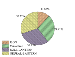
(d) Question Q3

Figure 8. (a) Length of output; (b)-(d) Responses to Question 1-3.

7.2. Experimental Results

Exp 1: Effect of diversifying text. First, we report the benefits brought by paraphrasing in neural-lantern. Table 4 reports the diversity of nl descriptions measured using Self-BLEU (SNC+19, ) (normalized to $0\sim 1$, a lower value indicates a higher diversity), which is widely adopted in machine translation tasks to measure diversity of the generated text in a language. Given the 1152 samples (544 from tpc-h, 608 from sdss) generated by rule-lantern, we apply the paraphrasing tools over each sample. As a result, each original sample (from rule-lantern) as well as its variations (generated by paraphrasing) form a group. We compute the diversity of each group and report the average over all 1152 groups. Notably, #Samples per group column refers to the number of samples in each group. Recall that we eliminate invalid or duplicate paraphrasing results. Hence, a few groups may have fewer samples than the theoretical values listed in the column. Clearly, paraphrasing is beneficial w.r.t diversity of nl descriptions. Next, we use the diversified samples (i.e., paraphrasing with (synonymous1, ; synonymous2, ; synonymous3, )) for training and evaluate the validation loss (i.e., cross entropy loss in Eq 12). Figure 6(a) plots the results. Observe that paraphrasing reduces the loss significantly.

Exp 2: Length of output. Although paraphrasing enables neural-lantern to generate descriptions with high diversity and low validation loss, does it make the descriptions verbose? We now report lengths of the nl descriptions generated by rule-lantern and neural-lantern to answer this. Figure 8(a) plots the lengths of the original sql statements in tpc-h as well as outputs of these two techniques. We observe that the length of a natural language description is, in fact, affected by the complexity and the number of relations in a sql statement, but not by the length of the statement. Importantly, neural-lantern injects variability without adversely impacting the length significantly compared to rule-lantern.

Exp 3: Effect of pre-trained word embeddings. Next, we compare the changes to the loss function by employing Word2Vec or otherwise. Figure 6(b) depicts the results. Observe that the adoption of pre-trained word vector can speed up training and significantly reduce the validation loss. We also notice that during training, the training set loss first decreases and then slowly increases (over 35 epochs). Hence we apply an early stopping strategy to prevent overfitting. Specifically, we terminate training when the training set loss fluctuation range is less than a threshold (e.g., 0.001).

Exp 4: Varying the pre-trained word vectors. We conduct a set of experiments to test the performance of neural-lantern by varying the pre-trained word vectors. In particular, we compare the following five approaches: QEP2Seq (with randomly initialized word embeddings), QEP2Seq+GloVe, QEP2Seq+Word2Vec, QEP2Seq+BERT, and QEP2Seq+ELMo. Figure 7(a) depicts the results in terms of sparse_categorical_accuracy (keras, ) averaged over all output sequences. For each output sequence with $m$ tokens, it can be calculated as $Acc=\frac{1}{m}\sum_{t=1}^{m}\mathbbm{1}(y_{t}=o)$. Observe that the training process is faster and the accuracy on the development set is higher when pre-trained vectors are adopted. As expected, the performance for the contextual embeddings (ELMo, BERT) are the best. In addition, using existing pre-trained word vectors, which are trained on large corpus such as Wikipedia, show superior results to our self-trained word vectors (referred to as self-trained in the figure), which are pre-trained on our rule-lantern output. This is expected as the dataset size is limited for the latter.

We also compare the impact of sharing and not sharing the weights between the Encoder and Decoder. The results are shown in Figure 7(b). Observe that the performances are comparable for models with pretrained embeddings.

Lastly, in line with existing Seq2Seq models, we adopt a measure that is widely used in machine translation task, i.e., BLEU (papineni2002bleu, ). For each specific approach of neural-lantern, we compute the BLEU score of its output with respect to the ground-truth and report the average over all samples. The results are presented in Table 5. Clearly, QEP2Seq+BERT demonstrates the most similar results with respect to the ground-truth.

Method	BLEU score (test set)
QEP2Seq	51.46
QEP2Seq+GloVe (pre-trained)	68.15
QEP2Seq+GloVe (self-trained)	57.01
QEP2Seq+Word2Vec (pre-trained)	64.01
QEP2Seq+Word2Vec (self-trained)	54.85
QEP2Seq+BERT (pre-trained)	73.73
QEP2Seq+ELMo (pre-trained)	71.67

Table 5. The performance of QEP2Seq (with beam size 4)

Steps	Training (over tpc-h and sdss samples)	Training for each epoch	SQL generation (1000 queries in imdb)	neural-lantern avg. response time	rule-lantern avg. response time
Time	825.60	16.51 [18.22]	0.77	0.216	0.015

Table 6. Efficiency (in sec).

Exp 5: Errors in neural-lantern. Observe that neither accuracy nor BLEU can justify the correctness (i.e., whether the translation make sense for human understanding) of the output of neural-lantern. Hence, we employ two smes to manually check the correctness of the nl descriptions. We uniformly sample 100 test samples randomly, and test whether the translated descriptions are correct. We find that 83 are correctly translated; another 13 has one wrong token; the remaining four contains 6-9 wrong tokens. In the next section, we shall investigate the impact of these descriptions on facilitating understanding of qeps among learners.

Exp 6: Efficiency. Table 6 reports the time cost of different components. Firstly, the average training time for each epoch is 16.51 (resp. 18.22) sec for $QEP2Seq+GloVe$ (resp. $QEP2Seq+ELMo$), which has the least (resp. largest) number of dimensions. Secondly, the average time taken to generate a nl description is less than a second.

7.3. User Study

We conducted a user study among cs undergraduate students who are taking the database course in an institution. 43 unpaid volunteers participating in the study. We utilized the gui of neuron (neuron, ) for presenting the input queries and output translations of lantern. Rest of the features (e.g., question answering module) of neuron are orthogonal to this work and hence were disabled. We presented a 10-min scripted tutorial of the gui describing how to use it. We then allowed the subjects to play with the tool for 15 min.

US 1: Survey. Each of the subjects was given the qeps corresponding to the queries in tpc-h/sdss and their natural language descriptions generated by rule-lantern and neural-lantern. The subjects were not informed on which description was generated by which technique. They were also given the corresponding json/xml and visual tree formats of qeps generated by PostgreSQL/SQL Server. The queries as well as outputs of different approaches were given in random order. They were allowed to take their own time to peruse the plans. After the completion of the task, the subjects were asked to fill up a survey form, which consists of a series of questions to understand the impact of various modes of qep on their understanding of how sql queries are executed. They were instructed that the outcomes of the survey have no bearing on their course grades. We now elaborate on the key results from the survey on tpc-h (results on sdss are qualitatively similar).

Q1: How easy it is to understand the query plan presented using each approach? Figure 8(b) shows the statistics with respect to the number of responses for this question. Each subject gave a rating in the Likert scale of 1-5. Observe that the lantern approach is the easiest format to understand. In particular, for both rule-lantern and neural-lantern, 58.1% of ratings are above 3 for both solutions. In comparison, there are 27.9% and 48.8% ratings above 3 for json and visual tree, respectively. Note that majority of the volunteers (41 out of 43) did not raise any issue with the length of the nl descriptions generated by lantern.

Q2: How well does lantern describe the query plans? Figure 8(c) reports the results. 86% (resp., 81.4%) of the respondents agree that the rule-lantern (resp., neural-lantern) does a good job in describing the query plans to facilitate understanding of query execution steps. Slightly higher agreement for the former is expected as hand-written rule-based technique is expected to be more accurate than the neural-based approach. We also observe that there is no significant impact of different pre-training models employed in neural-lantern (Figure 9(a)). This is not surprising as given the constrained nature of the problem (i.e., both input and output), large pretrained models like BERT has little scope to improve qualitatively.

We also study whether the diverse descriptions generated by lantern are confusing the volunteers. To this end, we generate 20 pairs of nl descriptions. 10 of these are positive examples where each pair is associated with the same sql query. That is, in each pair, the two descriptions are generated by rule-lantern and neural-lantern for the same qep. The remaining 10 pairs are negative examples where the two nl descriptions in each pair are from two different qeps. The 20 pairs are then given to the volunteers in random order and they were tasked to identify the positive example pairs. All volunteers correctly identified all the positive pairs.

Q3: Which query plan format do you prefer the most? Figure 8(d) reports the results. Both solutions of lantern are preferred the most. In particular, rule-lantern and neural-lantern receive similar preferences. On the other hand, very few, i.e., 11.63%, participants chose the textual format as the most preferred choice.

US 2: Impact of paraphrasing. We now conduct a user study to test the impact of incorporating paraphrasing in neural-lantern. The participants answer $Q2$ again but now they study the outputs of neural-lantern with (w) and without (w/o) usage of paraphrasing. The results are shown in Figure 9(b). The user experience of neural-lantern w/o paraphrasing is worse than with paraphrasing. In fact, when we eliminate the samples generated by paraphrasing, the results of neural-lantern contain many error tokens (e.g., missing filtering conditions) due to limited number of training samples and overfitting problem.

Method	Boredom index
	(not boring $\rightarrow$ extremely boring)
	1	2	3	4	5
rule-lantern	2	7	19	10	5
neural-lantern	6	11	22	3	1
neuron	2	8	16	11	6
lantern	6	12	21	2	2

Table 7. Impact on boredom.

US 3: Impact of habituation and boredom. The diversified translation of neural-lantern aims to mitigate the potential boredom suffered by subjects in using rule-lantern. To validate this issue, we presented a set of output generated by each approach in random order and asked the subjects to rate the degree of boredom (i.e., boredom index) they felt perusing these plans to understand qeps using the Likert scale of 1-5 (1 refers to no boredom and 5 refers to the highest degree of boredom). Note that boredom literature relies heavily on subjective self-report measures (MF+11, ). Table 7 reports the results (first two rows). 15 (gave scores above 3) out of 43 volunteers felt that the output of rule-lantern makes them bored and prone to skipping text due to repeated exposure of the same descriptions over multiple workloads. In comparison, only 4 volunteers (i.e., 9.3%) felt results of neural-lantern are boring.

In the above settings, the subjects perused the outputs of rule-lantern and neural-lantern separately in random order. In this experiment, we randomly mix the results of the two. In particular, we adopt 50 sql statements generated by (DBLP:conf/cidr/KipfKRLBK19, ) over imdb, each of which contains Hash Join and Aggregate operators. We use neural-lantern to generate every $4+f()$ output, where $f()$ is a pseudorandom function with uniform probability to output $\{-1,0,1\}$. Others are generated using rule-lantern. As a result, the volunteers are given 14 nl descriptions from neural-lantern, mixed with 36 output generated by rule-lantern. They are unaware of which output is generated by which technique. They were asked to mark outputs that make them feel bored to peruse and those which arouse their interests without compromising on understanding the qeps. We observe that not all descriptions are marked w.r.t boredom. Particularly, 21 (resp. 14) descriptions generated by rule-lantern (resp. neural-lantern) are marked. Out of them 2 (resp. 8) descriptions of rule-lantern (resp. neural-lantern) aroused interest. In summary, our proposed neural approach indeed alleviates the impact of boredom on learners.

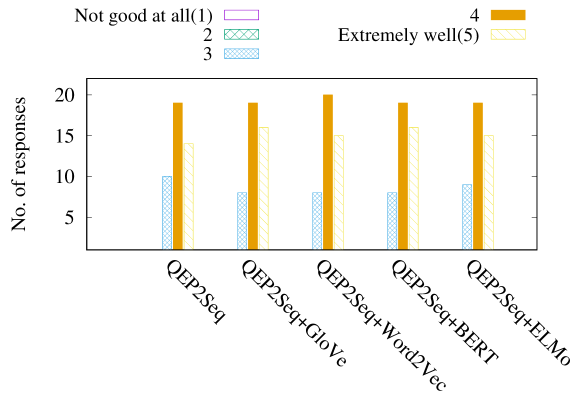
(a) Pre-trained models

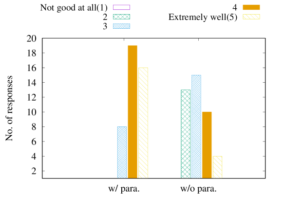
(b) Impact of paraphrasing.

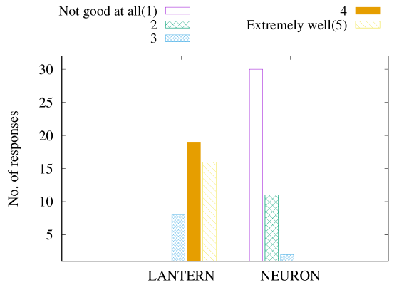
(c) lantern vs. neuron.

Figure 9. User study (contd.)

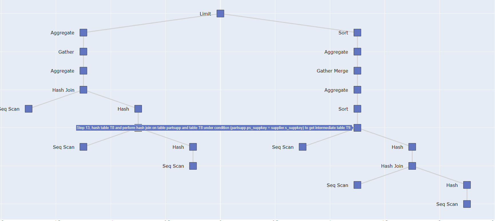
Figure 10. An example of visual tree-based nl presentation format.

US 4: Impact of incorrect token on comprehension. Recall that the neural-lantern may produce some wrong tokens in the test samples. Hence, we ask the volunteers to evaluate whether the existence of wrong tokens affect their understanding of qeps or mislead their understandings for the corresponding operators. Our study revealed that only 2 out of 43 think that the incorrect tokens are problematic for their understanding (gave a rating below 3).

US 5: Comparison with neuron (neuron, ). Lastly, we compare lantern with neuron (neuron, ). In order to compare the full features of lantern, we integrate rule-lantern and neural-lantern into a single framework for generating nl descriptions. Specifically, we track (qep, nl description) pairs viewed by each participants. By default, the nl description of each physical operator is generated using rule-lantern. Whenever an operator appeared more than a pre-defined frequency threshold (i.e., 5) in total in different qeps associated with a participant, neural-lantern is invoked to generate the description for the operator.

Firstly, we ask the volunteers how well these two frameworks describe the query execution steps for tpc-h and sdss workloads. Figure 9(c) reports the results. sdss on SQLServer is not supported by neuron as it is tightly integrated with PostgreSQL and does not expose a declarative framework like pool. The translation rules for various operators of PostgreSQL are hardcoded in neuron. Consequently, even if we allow neuron to use lantern’s parser for SQL Server to extract the operator tree from a given qep, none of the workloads of sdss is successfully translated as majority of operators of SQL Server have different names from those in PostgreSQL. Consequently, 41 out of 43 volunteers gave a score lower than 3 for neuron. Secondly, we compare the boredom index of neuron and lantern for tpc-h on PostgreSQL. As shown in the last two rows of Table 7, the volunteers found the output of rule-based neuron more boring than lantern. Thirdly, neuron (resp. lantern) takes on avg.0.015 sec (resp. 0.172 sec) to generate a nl description. The avg. length of the descriptions is 188.136 (resp. 188.318) tokens.

US 6: Presentation models. Recall that we use the presentation layer of neuron (neuron, ) in lantern. Specifically, nl descriptions are presented in document-style text format. In this experiment, we compare it with a visual tree-based nl presentation format by integrating the visual tree (Figure 4) with our nl description output. Specifically, the visual operator tree is shown by default and the nl description corresponding to each physical operator in the tree is added as an annotation to the corresponding node. A user can view the nl description of an operation by simply clicking on the corresponding node in the tree. An example is depicted in Figure 10. We ask the volunteers which of these two formats they prefer. Among the 43 participants, 38 of them selected the document-style text format. Majority of learners are taking the database course for the first time. They mentioned that they chose the simple document-style presentation format as the visual tree-based nl format incurs a mental overhead of integrating the nl descriptions associated with nodes and the sequence of steps depicted by the visual tree. In contrast, a text-based narration simply makes them read the text like a document (i.e., text book-style learning), which they are more familiar with.

8. Conclusions & Future Work

The quest for high-quality techniques for natural language interaction with rdbms have witnessed a rejuvenation due to tremendous progress in deep learning and natural language processing. This paper takes a concrete step towards this grand vision by presenting a domain-oblivious framework called lantern that generates natural language descriptions of qeps to aide learners taking a database systems course. lantern provides a new paradigm of efficiently specifying nl descriptions of physical operators through a declarative interface, a rule-based technique that utilizes such specifications to translate a qep to its nl description, and a psychology-inspired deep learning-based framework that adds diversity to the nl description in order to alleviate boredom among learners. We believe that lantern-generated descriptions of qeps complement its visual tree-based counterpart prevalent in commercial rdbms. Our user study indeed demonstrates the effectiveness of lantern in facilitating comprehension of qeps among learners. As part of future work, we wish to explore techniques to facilitate nl interaction with a query optimizer to comprehend qep selection.

Acknowledgments. Sourav S Bhowmick and Shafiq Joty are supported by AcRF Tier-1 Grant 2018-T1-001-134. Hui Li is supported by National Natural Science Foundation of China (No. 61972309). We would like to thank Dr Patricia Chen from NUS (Dept of Psychology) for her advice on research related to habituation and boredom. We also thank Zheng Li from Xidian University for contributing to the implementation of lantern on SQL Server.

References

- [1] BERT. https://storage.googleapis.com/bert_models/2018_10_18/uncased_L-12_H-768_A-12.zip.
- [2] ELMo.https://s3-us-west-2.amazonaws.com/allennlp/models/elmo/.
- [3] GloVe. https://nlp.stanford.edu/projects/glove/.
- [4] Habituation. Wikipedia. https://en.wikipedia.org/wiki/Habituation.
- [5] The IMDb database. https://relational.fit.cvut.cz/dataset/IMDb.
- [6] TensorFlow. https://www.tensorflow.org/api_docs/python/tf/keras/metrics/SparseCategoricalAccuracy.
- [7] Narration. Wikipedia. https://en.wikipedia.org/wiki/Narration.
- [8] Paraphrasing tool. https://paraphrasing-tool.com/.
- [9] Prepostseo paraphrasing tool. https://www.prepostseo.com/paraphrasing-tool.
- [10] Quillbot paraphraser. https://quillbot.com/.
- [11] SDSS dataset. https://www.skyserver.org/myskyserver/.
- [12] TPC-H benchmark. http://www.tpc.org.
- [13] Word2Vec. https://code.google.com/archive/p/word2vec/.
- [14] K. Andrej, F. F. Li. Deep Visual-Semantic Alignments for Generating Image Descriptions. IEEE Trans. Pattern Anal. Mach. Intell., 39(4): 664-676, 2017.
- [15] K. Affolter, K. Stockinger, A. Bernstein. A Comparative Survey of Recent Natural Language Interfaces for Databases. The VLDB Journal, 28(5): 793-819, 2019.
- [16] C. Baik, H. V. Jagadish, Y. Li. Bridging the Semantic Gap with SQL Query Logs in Natural Language Interfaces to Databases. In ICDE, 2019.
- [17] C. Baik, Z. Jin, M. J. Cafarella, H. V. Jagadish. Duoquest: A Dual-Specification System for Expressive SQL Queries. In SIGMOD, 2020.
- [18] F. Basik, et al. DBPal: A Learned NL-Interface for Databases. In SIGMOD, 2018.
- [19] D. Bahdanau, K. Cho, Y. Bengio. Neural machine translation by jointly learning to align and translate. In ICLR, 2015.
- [20] J. T. Cacioppo and R. E. Petty. Effects of Message Repetition and Position on Cognitive Response, Recall, and Persuasion. Journal of Personality and Social Psychology ,37, 1: 97-109, 1979.
- [21] S. Chatman. Story and Discourse: Narrative Structure in Fiction and Film. Cornell paperbacks, Cornell University Press, 1980.
- [22] S. Chaudhuri. An Overview of Query Optimization in Relational Systems. In PODS, 1998.
- [23] J. Devlin, M. Chang, K. Lee, K. Toutanova. Bert: Pre-training of deep bidirectional transformers for language understanding. ArXiv e-prints, 2018.
- [24] J. Gehring, M. Auli, D. Grangier, D. Yarats, Y. N. Dauphin. Convolutional Sequence to Sequence Learning. In ICML, 2017.
- [25] A. Graves, A. Mohamed, G. Hinton. Speech recognition with deep recurrent neural networks. In ICASSP, 2013.
- [26] A. A. Harrison and R. Crandall. Heterogeneity-homogeneity of Exposure Sequence and the Attitudinal Effect of Exposure. Journal of Personality and Social Psychology, 21, 2: 234-238, 1972.
- [27] M. R. Hastall and S. Knobloch-Westerwick. Severity, Efficacy, and Evidence Type as Determinants of Health Message Exposure. Health Communication, 28, 4: 378-388, 2013.
- [28] G. Hervet, K. Guerard, S. Tremblay, M. Saber Chtourou. Is Banner Blindness Genuine? Eye Tracking Internet Text Advertising. Applied Cognitive Psychology, 25, 5: 708-716, 2011.
- [29] A. B. Hill, R. E. Perkins. Towards a Model of Boredom. British Journal of Psychology, 76, 1985.
- [30] H. Kim, B.-H. So, W.-S. Han. H. Lee. Natural Language to SQL: Where Are We Today? PVLDB, 13(10), 2020.
- [31] A. Kipf, T. Kipf, B. Radke, V. Leis, P. A. Boncz, A. Kemper. Learned Cardinalities: Estimating Correlated Joins with Deep Learning. In CIDR, 2019.
- [32] A. Kokkalis, P. Vagenas, A. Zervakis, A. Simitsis, G. Koutrika, Y. E. Ioannidis. Logos: A System for Translating Queries into Narratives. In SIGMOD, 2012.
- [33] F. Li, H. V. Jagadish. NaLIR: An Interactive Natural Language Interface for Querying Relational Databases. In SIGMOD, 2014.
- [34] F. Li, H. V. Jagadish. Constructing an Interactive Natural Language Interface for Relational Databases. PVLDB, 8(1), 2014.
- [35] Y. Li, I. Chaudhuri, H. Yang, S. P. Singh, H. V. Jagadish. DaNaLIX: a domain-adaptive natural language interface for querying XML. In SIGMOD, 2007.
- [36] S. Liu, et al. NEURON: Query Optimization Meets Natural Language Processing For Augmenting Database Education. In SIGMOD, 2019.
- [37] K. B. Mercer-Lynn ,D. B. Flora, S. A. Fahlman, J. D. Eastwood. The Measurement of Boredom: Differences between Existing self-report Scales. Assessment, 2011.
- [38] T. Mikolov, K. Chen, G. Corrado, J. Dean. Efficient estimation of word representations in vector space. ArXiv e-prints, 2013.
- [39] W. L. Mikulas., S. J. Vodanovich. The Essence of Boredom. The Psychological Record, 43, 1993.
- [40] M. Luong, H. Pham, C. Manning. Effective approaches to attention-based neural machine translation. ArXiv e-prints, 2015.
- [41] J. F. O’Hanlon. Boredom: Practical Consequences and a Theory. Acta Psychologica, 49, 53-82, 1981.
- [42] F. El Outa, M. Francia, P. Marcel, V. Peralta, P. Vassiliadis. Towards a Conceptual Model for Data Narratives. In ER, 2020.
- [43] K. Papineni, S. Roukos, T. Ward, W. Zhu. BLEU: a method for automatic evaluation of machine translation. In ACL, 2002.
- [44] J. Pennington, R. Socher, C. Manning. Glove: Global vectors for word representation. In EMNLP, 2014.
- [45] M. Peters, M. Neumann, M. Iyyer, M. Gardner, C. Clark, K. Lee, L. Zettlemoyer. 2018. Deep contextualized word representations. In NAACL, 2018.
- [46] D. Saha, A. Floratou, et al. ATHENA: An Ontology-Driven System for Natural Language Querying over Relational Data Stores. PVLDB, 9(12), 2016.
- [47] D. W. Schumann, R. E. Petty,D. S. Clemons. Predicting the Effectiveness of Different Strategies of Advertising Variation: A Test of the Repetition-Variation Hypotheses. Journal of Consumer Research, 17, 2: 192, 1990.
- [48] A. See, P. J. Liu, C. D. Manning. Get to the point: Summarization with pointer-generator networks. In ACL, 2017.
- [49] R. Shu, H. Nakayama, K. Cho. Generating Diverse Translations with Sentence Codes. In ACL, 2019.
- [50] I. Sutskever, O. Vinyals, Q. V Le. Sequence to Sequence Learning with Neural Networks. In NeurIPS, 2014.
- [51] USESCO Insititute of Lifelong Learning. UNESCO Global Network of Learning Cities. Accessible at https://uil.unesco.org/lifelong-learning/learning-cities, 2019.
- [52] P. Utama, N. Weir, F. Basik, C. Binnig, U. Cetintemel, B. Hattasch, A. Ilkhechi, S. Ramaswamy, and A. Usta. An End-to-end Neural Natural Language Interface for Databases. ArXiv e-prints, Apr. 2018.
- [53] A. Vaswani, N. Shazeer, N. Parmar, J. Uszkoreit, L. Jones, A. N Gomez, Ł. Kaiser, I. Polosukhin. Attention is all you need. In NeurIPS, 2017.
- [54] O. Vinyals, Q. Le. A neural conversational model. CoRR, abs/1506.05869, 2015.
- [55] O. Vinyals, A. Toshev, S. Bengio, D. Erhan. Show and tell: A neural image caption generator. In CVPR, 2015.
- [56] J. D. Watt , S. J. Vodanovich. Boredom Proneness and Psychosocial Development. The Journal of Psychology, 133/3, pp. 303-314, 1999.
- [57] Nathaniel Weir, Prasetya Utama. Bootstrapping an End-to-End Natural Language Interface for Databases. In SIGMOD, 2019.
- [58] R. J. Williams and D. Zipser. A learning algorithm for continually running fully recurrent neural networks. Neural Computation, 1(2):270-280, 1989.
- [59] F. Wu, A. Fan, A. Baevski, Y. Dauphin, M. Auli. Pay less attention with lightweight and dynamic convolutions. In ICLR, 2019.
- [60] B. Xu, R. Cai, Z. Zhang, X. Yang, Z. Hao, Z. Li, Z. Liang. NADAQ: Natural Language Database Querying Based on Deep Learning. IEEE Access, 7: 35012-35017, 2019.
- [61] P. Yin, Z. Lu, H. Li, and B. Kao. Neural Enquirer: Learning to Query Tables in Natural Language. In IJCAI, 2016
- [62] T. Yu, R. Zhang, K. Yang, M. Yasunaga, D. Wang, Z. Li, J. Ma, I. Li, Q. Yao, S. Roman, Z. Zhang, and D. R. Radev. Spider: A Large-scale Human-labeled Dataset for Complex and Cross-domain Semantic Parsing and Text-to-SQL Task. CoRR, abs/1809.08887, 2018.
- [63] T. Yu, R. Zhang, et al. CoSQL: A Conversational Text-to-SQL Challenge Towards Cross-Domain Natural Language Interfaces to Databases. In EMNLP/IJCNLP, 2019.
- [64] W. Zheng, H. Cheng, L. Zou, J. X. Yu, K. Zhao. Natural Language Question/Answering: Let Users Talk With The Knowledge Graph. In CIKM, 2017.
- [65] V. Zhong, C. Xiong, and R. Socher. Seq2sql: Generating Structured Queries from Natural Language using Reinforcement Learning, CoRR abs/1709.00103, 2017.