A Difference-of-Convex Cutting Plane Algorithm for Mixed-Binary Linear Program

Abstract

In this paper, we propose a cutting plane algorithm based on DC (Difference-of-Convex) programming and DC cut for globally solving Mixed-Binary Linear Program (MBLP). We first use a classical DC programming formulation via the exact penalization to formulate MBLP as a DC program, which can be solved by DCA algorithm. Then, we focus on the construction of DC cuts, which serves either as a local cut (namely type-I DC cut) at feasible local minimizer of MBLP, or as a global cut (namely type-II DC cut) at infeasible local minimizer of MBLP if some particular assumptions are verified. Otherwise, the constructibility of DC cut is still unclear, and we propose to use classical global cuts (such as the Lift-and-Project cut) instead. Combining DC cut and classical global cuts, a cutting plane algorithm, namely DCCUT, is established for globally solving MBLP. The convergence theorem of DCCUT is proved. Restarting DCA in DCCUT helps to quickly update the upper bound solution and to introduce more DC cuts for lower bound improvement. A variant of DCCUT by introducing more classical global cuts in each iteration is proposed, and parallel versions of DCCUT and its variant are also designed which use the power of multiple processors for better performance. Numerical simulations of DCCUT type algorithms comparing with the classical cutting plane algorithm using Lift-and-Project cuts are reported. Tests on some specific samples and the MIPLIB 2017 benchmark dataset demonstrate the benefits of DC cut and good performance of DCCUT algorithms.

1 Introduction

Mixed-Binary Linear Program, namely MBLP, is a well-known NP-hard problem raised as one of the Karp’s $21$ NP-complete problems in Karp1972 . The general MBLP is given by:

$$\begin{split}\min\quad&f(x,y)\overset{\mathrm{def}}{=}c^{\top}x+d^{\top}y\\ \text{s.t.}\quad&(x,y)\in\mathcal{K}\\ \quad&x\in\{0,1\}^{n},\end{split}$$ (MBLP)

where $n\in\mathbb{N}^{*}$ is the number of binary variables, $q\in\mathbb{N}$ is the number of continuous variables (i.e., the problem has at least one binary variable, and could have no continuous variable), the coefficients $c\in\mathbb{R}^{n}$ and $d\in\mathbb{R}^{q}$, the set $\mathcal{K}$ is supposed to be a nonempty compact polyhedral convex set of $\mathbb{R}^{n}\times\mathbb{R}^{q}$ in form of

$$\mathcal{K}\overset{\mathrm{def}}{=}\{(x,y)\in[0,1]^{n}\times[0,\bar{y}]~{}|~{}Ax+By\leq b\},$$ (1)

where $m\in\mathbb{N}$ is the number of linear constraints, the coefficients $A\in\mathbb{R}^{m\times n}$, $B\in\mathbb{R}^{m\times q}$, $b\in\mathbb{R}^{m}$, and $\bar{y}\in\mathbb{R}_{+}^{q}$. Note that any (MBLP) with negative variables in $y$ can be converted in form of positive variables only by classical standardization of linear program. The set of feasible solutions of (MBLP), denoted by $\mathcal{S}$, is a subset of $\mathcal{K}$ and assumed to be nonempty.

The researches on MBLP can go back to the early 1950s with the birth of combinatorial integer programming in investigating the well-known traveling salesman problem (TSP) initialed by several pioneers: Hassler Whitney, George Dantzig, Julia Robinson, Ray Fulkerson, and Selmer Johnson Robinson1949 ; Dantzig1954 ; Dantzig1959 . There are very rich literatures on MBLP over the past seven decades, focusing either on theory and algorithms, or on real-world applications. Two classes of approaches exist for general MBLP: Exact methods and Heuristic methods. The exact methods consist of two typical approaches: continuous approaches and combinatorial approaches. The continuous approaches first reformulate the MBLP as nonconvex continuous optimization problems by replacing binary variables as continuous ones, then a classical nonlinear optimization algorithm such as Newton-type method Bertsekas1997 , gradient-type method Bertsekas1997 , difference-of-convex approache Le2001 ; Niu2008 ; Niu2010 ; Pham2016 ; Niu2018 , and dynamical system approach Niu2019DiscreteDS is used for numerical solutions. The advantage of this type of methods is inexpensive local optimization procedure which helps to find quickly a computed solution with guaranteed local optimality at best. The combinatorial approaches exploit techniques such as cutting-plane Gomory1958 ; Balas1971 ; Balas1993 ; Cornuejols2008 , branch-and-bound/branch-and-cut/branch-and-price Dantzig1959 ; Efroymson1966 ; Kolesar1967 , and column generation Benders1962 etc., which aim at dividing big problems into smaller problems that are easier to solve with reduced problem size and shrinked search region. These methods can find exact global optimal solution for problems with moderate size. But due to the NP-hardness, they are often very computationally expensive for large-scale cases. To quickly find feasible solutions, heuristic methods are often preferred, such as genetic algorithms, simulated annealing, ant colony, tabu search, and neural networks etc. These approaches mimic activities in nature for searching potentially good candidates without guaranteeing to be optimal, which aim at providing a satisfactory computed solution (may not even be a local optimum) within a reasonable time, but the optimality of the computed solution is not qualified. These methods are often used to provide good feasible initial candidates, or for hard problems in which no exact method works to find any solution. All of these techniques have been widely used in many modern integer/mixed-integer optimization solvers such as GUROBI Gurobi , CPLEX Cplex , BARON Sahinidis1996 , MOSEK Mosek , MATLAB intlinprog MATLAB , and some open-source solvers as SCIP Achterberg2009 , BONMIN Bonmin and COUENNE Belotti2009 .

In our paper, we are interested in developing a hybrid approach combining techniques in continuous approach (DCA) and combinatorial approach (cutting planes) for globally solving MBLP. Concerning continuous approach, we are interested in DCA which is a promising algorithm to provide good local optimal solution with many successful practical applications (see e.g., LeThi2005 ; LeThi2018 ; Pham1997 ; Pham1998 ). Applying DCA to binary linear program is first introduced in LeThi2001 by H.A. Le Thi and D.T. Pham, then the general cases with mixed-integer linear/nonlinear optimization are studied by Y.S. Niu, D.T. Pham et al. (see e.g., Niu2008 ; Niu2010 ; Niu2011 ) where the integer variables are not supposed to be binary. These methods are based on continuous representation techniques for integer set, exact penalty theorem, DCA and branch-and-bound. There are various applications of this kind of approaches including sentence compression niu2021sentence , scheduling paper_lethi_2009a , network optimization Schleich2012 , cryptography paper_lethi_2009c and finance paper_lethi_2009b ; Pham2016 etc. Recently, Y.S. Niu (the first author of the paper) released an open-source optimization solver, combining DCA with parallel branch-and-bound framework, namely PDCABB Niu2018 (code available on Github PDCABB ), for general mixed-integer nonlinear optimization. Concerning combinatorial approach, we focus on DC cutting plane technique constructed at local minimizers provided by DCA. DC cut is proposed in Nguyen2006 with a DCA-CUT algorithm, and applied in several real-world problems such as the bin-parking problem Babacar2012 and the scheduling problem Quang2010 . However, DCA-CUT algorithm is not well-constructed in the sense that there exist some cases, often encountered in practice, where DC cut is unconstructible. Due to this drawback, there are several works (e.g., Niu2012 ; Quang2010 ) combining constructible DC cuts, DCA and branch-and-bound for global optimal solutions of MBLP.

Our contributions are: (1) Revisit DC cutting plane (cf. DC cut) techniques and provide more theoretical results on constructible and unconstructible cases for DC cuts. As a result, two types of DC cuts: type-I DC cut (local DC cut) and type-II DC cut (global DC cut) are established at local minimizers of DC programs; (2) Propose using classical global cuts, such as the Lift-and-Project (L&P) cut, Gomory’s mixed-integer (GMI) cut and mixed integer rounding (MIR) cut, when DC cut is unconstructible, to cut off infeasible point; (3) Establish a cutting plane algorithm, namely DCCUT algorithm, combining DC cut and classical global cuts for globally solving MBLP. The convergence theorem of DCCUT is also proved. (4) Implement DCCUT algorithm, its variant DCCUT-V1 with more cutting planes in each iteration, and parallel algorithms (P-DCCUT and P-DCCUT-V1) in a MATLAB toolbox and shared on Github https://github.com/niuyishuai/DCCUT.

The rest of the paper is organized as follows: In Section 2, we presents general results on DC programming formulation and DCA for MBLP. In Section 3, we investigate in detail the DC cut techniques, and briefly introduce the classical Lift-and-Project cut. The proposed DCCUT algorithm and its variant (with and without parallelism) are established in Section 4. Numerical results are reported in Section 5. Concluding remarks and related questions are discussed in the last section.

2 DC programming approach for MBLP

In this section, we first introduce some backgrounds on Difference-of-Convex (DC) programming and DCA algorithm for readers to better understand the fundamental tool used in this paper, then we present the DC formulation for problem (MBLP) based on exact penalty theorem, and apply DCA to solve it.

2.1 Notations

Let $\mathbb{R}^{l}$ denote the $l$-dimensional Euclidean space equipped with the standard inner product $\langle\cdot,\cdot\rangle$ and the induced norm $\|\cdot\|$. For any extended real-valued function $\phi:\mathbb{R}^{l}\rightarrow(-\infty,+\infty]$, the effective domain is given by $\operatorname{dom}\phi\overset{\mathrm{def}}{=}\{x\in\mathbb{R}^{l}~{}|~{}\phi(x)<+\infty\}$. If $\operatorname{dom}\phi\neq\emptyset$, then $\phi$ is called a proper function. The directional derivative of $\phi$ at $x\in\operatorname{dom}\phi$ along a direction $d\in\mathbb{R}^{l}$ is defined by

$$\phi^{\prime}(x;d)=\lim\limits_{\tau\downarrow 0}\frac{\phi(x+\tau d)-\phi(x)}{\tau}.$$

The epigraph of $\phi$ is defined by $\operatorname{epi}\phi\overset{\mathrm{def}}{=}\{(x,t)\in\mathbb{R}^{l}\times\mathbb{R}~{}|~{}\phi(x)\leq t\}$, and $\phi$ is called a closed (resp. convex) function if $\operatorname{epi}\phi$ is closed (resp. convex). In particular, $\phi$ is called a polyhedral function if $\operatorname{epi}\phi$ is a polyhedral convex set. Given a nonempty polyhedral convex set $\mathcal{K}\subseteq\mathbb{R}^{l}$, the vertex set of $\mathcal{K}$ is denoted by $V(\mathcal{K})$ whose cardinality $|V(\mathcal{K})|$ is clearly finite. The set of all proper, closed and convex functions on $\mathbb{R}^{l}$ is denoted by $\Gamma_{0}(\mathbb{R}^{l})$, which is a convex cone; and $\text{DC}(\mathbb{R}^{l})\overset{\mathrm{def}}{=}\Gamma_{0}(\mathbb{R}^{l})-\Gamma_{0}(\mathbb{R}^{l})$ is the set of DC (Difference-of-Convex) functions (under the convention that $(+\infty)-(+\infty)=+\infty$), which is in fact a vector space spanned by $\Gamma_{0}(\mathbb{R}^{l})$. Let $\phi$ be a proper convex function, the subdifferential of $\phi$ at $x$ is defined by:

$$\partial\phi(x)\overset{\mathrm{def}}{=}\{u\in\mathbb{R}^{l}~{}|~{}\phi(y)\geq\phi(x)+\langle u,y-x\rangle\;\text{for all}\;y\in\mathbb{R}^{l}\},$$

where any point in $\partial\phi(x)$ is called a subgradient of $\phi$ at $x$. Clearly, $\partial\phi(x)\neq\emptyset$ implies that $x\in\operatorname{dom}\phi$; particularly, if $\phi$ is differentiable at $x\in\operatorname{dom}\phi$, then $\partial\phi(x)$ is reduced to a singleton, i.e., $\partial\phi(x)=\{\triangledown\phi(x)\}$.

Let $\mathcal{C}\subseteq\mathbb{R}^{l}$ be a nonempty convex set, the indicator function of $\mathcal{C}$, denoted by $\chi_{\mathcal{C}}:\mathbb{R}^{l}\to\mathbb{R}$, equals to $0$ on $\mathcal{C}$ and $+\infty$ otherwise. For any $x\in\mathcal{C}$, the set $\mathcal{N}_{\mathcal{C}}(x)\overset{\mathrm{def}}{=}\{d\in\mathbb{R}^{l}~{}|~{}\langle d,y-x\rangle\leq 0\text{ for all }y\in\mathcal{C}\}$ denotes the normal cone of $\mathcal{C}$ at $x$, and $\mathcal{N}_{\mathcal{C}}(z)=\emptyset$ if $z\notin\mathcal{C}$ by convention.

2.2 DC program and DCA

The standard DC program is defined by

$$\alpha=\text{min}\;\{\phi(x)\overset{\mathrm{def}}{=}\phi_{1}(x)-\phi_{2}(x):x\in\mathbb{R}^{l}\}, P_{dc}$$ ()

where $\phi_{1}$ and $\phi_{2}$ belong to $\Gamma_{0}(\mathbb{R}^{l})$ and $\phi\in\text{DC}(\mathbb{R}^{l})$. The objective value $\alpha$ is assumed to be finite, so that $\emptyset\neq\operatorname{dom}\phi_{1}\subset\operatorname{dom}\phi_{2}$. A point $x^{*}$ is called a critical point of problem ($P_{dc}$) if $\partial\phi_{1}(x^{*})\cap\partial\phi_{2}(x^{*})\neq\emptyset$, and a strongly critical point of problem ($P_{dc}$) if $\emptyset\neq\partial\phi_{2}(x^{*})\subset\partial\phi_{1}(x^{*})$, i.e., $\phi^{\prime}(x^{*};x-x^{*})\geq 0$ for all $x\in\operatorname{dom}\phi_{1}$. Clearly, a strongly critical point must be a critical point, but the converse is not true in general. Note that in nonconvex optimization, a critical point or a strongly critical point of problem ($P_{dc}$) may not be a local minimizer. We have some particular cases in which a stationary point is guaranteed to be a local minimizer of $\phi$, e.g., if $\phi$ is locally convex at a critical point $x^{*}$, then $x^{*}$ must be a local minimizer of $\phi$. The readers can refer to Pang2016 for more details about the stationarity.

A well-known DC algorithm, namely DCA, for ($P_{dc}$) was first introduced by D.T. Pham in 1985 as an extension of the subgradient method, and extensively developed by H.A. Le Thi and D.T. Pham since $1994$ (see e.g., Pham1997 ; Pham1998 ; LeThi2005 ; LeThi2018 ). Broadly speaking, DCA is not one single algorithm, it is a philosophy to solve DC programs by a sequence of convex ones. A classical DCA gives:

$$x^{k+1}\in\operatorname{argmin}\{\phi_{1}(x)-\langle x,y^{k}\rangle~{}|~{}x\in\mathbb{R}^{l}\}$$

with $y^{k}\in\partial\phi_{2}(x^{k})$. This convex program is derived from minimizing a convex overestimation of $\phi$ at iterate $x^{k}$, denoted by $\phi^{k}$, constructed by linearizing $\phi_{2}$ at $x^{k}$ as

$$\forall x\in\mathbb{R}^{l},~{}\phi(x)=\phi_{1}(x)-\phi_{2}(x)\leq\phi_{1}(x)-(\phi_{2}(x^{k})+\langle x-x^{k},y^{k}\rangle)\overset{\mathrm{def}}{=}\phi^{k}(x),$$

where $y^{k}\in\partial\phi_{2}(x^{k})$. The principal of DCA can be viewed geometrically in Niu2010 ; Niu2014 . See below the classical DCA for problem ($P_{dc}$):

1

2Initialization: Choose $x^{0}\in\operatorname{dom}(\partial\phi_{2})$.

3Iterations: For $k=0,1,2,\dots$

4Compute $y^{k}\in\partial\phi_{2}(x^{k})$;

Find $x^{k+1}\in\operatorname{argmin}\{\phi_{1}(x)-\langle x,y^{k}\rangle,x\in\mathbb{R}^{l}\}.$

DCA for problem ($P_{dc}$)  1

Remark 1

To make sure that DCA can be implemented, it is required that at iteration $k$ both $\partial\phi_{2}(x^{k})$ and $\operatorname{argmin}\{\phi_{1}(x)-\langle x,y^{k}\rangle,x\in\mathbb{R}^{l}\}$ are nonempty.

The next theorem summarizes some important convergence results of DCA.

Theorem 2.1 (Convergence of DCA Pham1997 ; LeThi2005 )

Let $\{x^{k}\}$ and $\{y^{k}\}$ be bounded sequences generated by DCA Algorithm 1 for problem ($P_{dc}$), and suppose that $\alpha$ is finite, then

1. The sequence $\{\phi(x^{k})\}$ is decreasing and bounded below.

2. Any limit point of $\{x^{k}\}$ is a critical point of problem ($P_{dc}$).

3. If either $\phi_{1}$ or $\phi_{2}$ is polyhedral, then problem $\eqref{primal1}$ is called polyhedral DC program, and DCA is terminated in finitely many iterations.

4. If $x^{*}$ is a critical point generated by DCA, and if $\phi$ is locally convex at $x^{*}$, then $x^{*}$ is a local minimizer of $\phi$.

More theoretical results of DC program and DCA can be found in Pham1997 ; Pham1998 ; LeThi2005 ; LeThi2018 and the references therein.

2.3 DC formulation for (MBLP)

We will show that problem (MBLP) can be equivalently represented as a standard DC program in form of ($P_{dc}$).

Firstly, we will use continuous representation technique to reformulate the binary set $\{0,1\}^{n}$ as a set involving continuous variables and continuous functions only. A classical way is using a nonnegative concave function $p$ over $[0,1]^{n}$ to rewrite the binary set as:

$$\{0,1\}^{n}=\{x\in[0,1]^{n}~{}|~{}p(x)\leq 0\}.$$

Then

$$\mathcal{S}=\{(x,y)\in\mathcal{K}~{}|~{}p(x)\leq 0\},$$

where the polyhedral convex set $\mathcal{K}$ is defined in (1). There are many alternative functions for $p$, such as the quadratic function $p:x\mapsto\sum_{i=1}^{n}x_{i}(1-x_{i})$ and the piecewise linear function $p:x\mapsto\sum_{i=1}^{n}\min\{x_{i},1-x_{i}\}$. The main differences between these two functions are: the quadratic function is differentiable and concave over $[0,1]^{n}$; while the piecewise linear function is not differentiable at some points (e.g., the points with some coordinates as $0.5$) but it is locally convex (specifically, locally affine) at any differentiable point over $[0,1]^{n}$. In this paper, we will use the latter function since the local convexity is crucial to identify a local minimizer for a critical point returned by DCA.

Next, we will use the well known exact penalty theorem penalty1999 ; LeThi2012 to reformulate problem (MBLP) as a standard DC program. The exact penalty theorem is stated as follows:

Theorem 2.2 (See e.g., penalty1999 ; LeThi2012 )

Let $p(x)=\sum_{i=1}^{n}\min\{x_{i},1-x_{i}\}$, then there exists a finite number $t_{0}\geq 0$ such that for all $t>t_{0}$, problem (MBLP) is equivalent to

$$\alpha_{t}=\min\{f(x,y)+tp(x)~{}|~{}(x,y)\in\mathcal{K}\}. P_{t}$$ ()

The equivalence means that problems (MBLP) and ($P_{t}$) have the same set of global optimal solutions. The penalty parameter $t_{0}$ can be computed by:

$$t_{0}=\frac{\min\{f(x,y)~{}|~{}(x,y)\in\mathcal{S}\}-\alpha_{0}}{m},$$ (2)

where $m=\min\{p(x)~{}|~{}(x,y)\in V(\mathcal{K}),p(x)>0\}$ under the convention that $m=+\infty$ if $\{(x,y)\in V(\mathcal{K})~{}|~{}p(x)>0\}=\emptyset$ and $\frac{1}{+\infty}=0$. In practice, computing $t_{0}$ is difficult since both $\min\{f(x,y)~{}|~{}(x,y)\in\mathcal{S}\}$ and $\min\{p(x)~{}|~{}(x,y)\in V(\mathcal{K}),p(x)>0\}$ are nonconvex optimization problems which are difficult to be solved, while the computation of $\alpha_{0}$ is easy which just need to solve a linear program. Note that if the set of vertices $V(\mathcal{K})$ is known, then it will be much easier to find an upper bound for $t_{0}$, since $m$ can be easily solved by checking all points in $V(\mathcal{K})$, and we just need to find a feasible solution of $\min\{f(x,y)~{}|~{}(x,y)\in\mathcal{S}\}$ to get an upper bound for $t_{0}$. In numerical simulations, the parameter $t$ is often fixed arbitrarily to be a large positive number.

Supposing that $t$ is large enough, then problem ($P_{t}$) is in fact a concave minimization problem over a polyhedral convex set which is equivalent to a standard DC program as:

$$\min\{\tau_{t}(x,y)~{}|~{}(x,y)\in\mathbb{R}^{n}\times\mathbb{R}^{q}\},$$

where

$$\tau_{t}(x,y)=\underbrace{\chi_{\mathcal{K}}(x,y)}_{g(x,y)}-[\underbrace{-f(x,y)-tp(x)}_{h(x,y)}]$$

is a DC function in $\text{DC}(\mathbb{R}^{n}\times\mathbb{R}^{q})$, and $g$ and $h$ are $\Gamma_{0}(\mathbb{R}^{n}\times\mathbb{R}^{q})$ functions.

2.4 DCA for Problem ($P_{t}$)

To apply DCA for problem ($P_{t}$), we first compute $\partial h$ by

$$\partial h(x,y)=(-c+tz,-d),\text{ where }z_{i}=\begin{cases}1&\text{, if }x_{i}>\frac{1}{2};\\ s\in[-1,1]&\text{, if }x_{i}=\frac{1}{2};\\ -1&\text{, if }x_{i}<\frac{1}{2};\end{cases}$$

for all $i=1,\ldots,n$. Then, we can compute $(x^{k+1},y^{k+1})$ from $(x^{k},y^{k})$ by solving the linear program via simplex method:

$$(x^{k+1},y^{k+1})\in\operatorname{argmin}\{-\langle(v^{k},w^{k}),(x,y)\rangle:(x,y)\in\mathcal{K}\},$$

where $(v^{k},w^{k})\in\partial h(x^{k},y^{k})$. Note that only $v^{k}$ is updated in each iteration and $w_{k}$ is fixed to $-d$.

DCA could be terminated if $|\tau_{t}(x^{k+1},y^{k+1})-\tau_{t}(x^{k},y^{k})|/(|\tau_{t}(x^{k+1},y^{k+1})|+1)\leq\varepsilon_{1}$ and/or $\|(x^{k+1},y^{k+1})-(x^{k},y^{k})\|/(\|(x^{k+1},y^{k+1})\|+1)\leq\varepsilon_{2}$ where $\varepsilon_{1}$ and $\varepsilon_{2}$ are given tolerances.

The detailed DCA for problem ($P_{t}$) is summarized as follows.

Input: Initial point $(x^{0},y^{0})\in\mathbb{R}^{n}\times\mathbb{R}^{q}$, small tolerances $\varepsilon_{1}>0$ and $\varepsilon_{2}>0$.

Output: Computed solution $(x^{*},y^{*})$ and computed optimal value $\tau^{*}$.

1

2Initialization: Set $k\leftarrow 0$.

3Step 1: Compute $(v^{k},w^{k})\in\partial h(x^{k},y^{k})$.

4Step 2: Solve the linear program via the simplex algorithm:

$$(x^{k+1},y^{k+1})\in\operatorname{argmin}\{-\langle(v^{k},w^{k}),(x,y)\rangle:(x,y)\in\mathcal{K}\};$$

5$\Delta\tau\leftarrow|\tau_{t}(x^{k+1},y^{k+1})-\tau_{t}(x^{k},y^{k})|/(|\tau_{t}(x^{k+1},y^{k+1})|+1);$

6$\Delta X\leftarrow\|(x^{k+1},y^{k+1})-(x^{k},y^{k})\|/(\|(x^{k+1},y^{k+1})\|+1);$

7Step 3: Stopping check:

8 if $\Delta\tau\leq\varepsilon_{1}$ or $\Delta X\leq\varepsilon_{2}$ then

9       $(x^{*},y^{*})\leftarrow(x^{k+1},y^{k+1})$; $\tau^{*}\leftarrow\tau_{t}(x^{k+1},y^{k+1})$; return;

10else

11       $k\leftarrow k+1$; Goto Step 1;

12 end

DCA for problem ($P_{t}$) 2

Remark 2

1. In Step 1, the selection of $(v^{k},w^{k})$ in $\partial h(x^{k},y^{k})$ may not be unique. When $x_{i}^{k}=1/2$, we can choose $u_{i}$ randomly in $[-1,1]$.

2. We suggest using the well-known simplex algorithm for solving the linear program required in Step 2 to find a vertex solution. It is easy to see that there exists optimal solution of (MBLP) in $V(\operatorname{co}(\mathcal{S}))$ (set of vertices of convex hull of $\mathcal{S}$), therefore, only vertex solutions are of our interests.

The convergence theorem of DCA for problem ($P_{t}$) is summarized in Theorem 2.1. Note that problem ($P_{t}$) is a polyhedral DC program, thus DCA will converge in finitely many iterations. Concerning the local optimality of the computed solution returned by DCA, we have the following Proposition:

Proposition 1

Let $(x^{*},y^{*})$ be a computed solution of problem ($P_{t}$) returned by DCA, if $x_{i}^{*}\neq 1/2,\forall i=1,\cdots,n$, then $(x^{*},y^{*})$ is a local minimizer of ($P_{t}$).

Proof

The function $h$ is differentiable at $(x^{*},y^{*})$ since all entries of $x^{*}$ are different to $\frac{1}{2}$, then $\partial h(x^{*},y^{*})$ is reduced to a singleton $\{\nabla h(x^{*},y^{*})\}$. Based on Theorem 2.1, $(x^{*},y^{*})$ is a critical point, then

$$\partial g(x^{*},y^{*})\cap\partial h(x^{*},y^{*})=\{\nabla h(x^{*},y^{*})\}\subset\partial g(x^{*},y^{*})=\mathcal{N}_{\mathcal{K}}(x^{*},y^{*}),$$

we get

$$\langle\nabla(-h)(x^{*},y^{*}),(x,y)-(x^{*},y^{*})\rangle\geq 0,\;\forall(x,y)\in\mathcal{K}.$$ (3)

By the local convexity (locally affine) of $-h$ at $(x^{*},y^{*})$, there exists a neighborhood $U$ of $(x^{*},y^{*})$ such that

$$(-h)(x,y)\geq(-h)(x^{*},y^{*})+\langle\nabla(-h)(x^{*},y^{*}),(x,y)-(x^{*},y^{*})\rangle,\;\forall(x,y)\in U.$$ (4)

Combining (3) and (4), we obtain

$$(-h)(x,y)\geq(-h)(x^{*},y^{*}),\forall(x,y)\in U\cap\mathcal{K}.$$

Therefore, $(x^{*},y^{*})$ is a local minimizer of problem ($P_{t}$). ∎

Note that if there exists $x_{i}^{*}=1/2$, then the critical point $(x^{*},y^{*})$ obtained by DCA may not be a local minimizer. For example, let $f(x,y)=0,\forall(x,y)\in\mathcal{K}=[0,1/2]^{n}\times\{0_{\mathbb{R}^{q}}\}$, then at the initial point $(x^{0},y^{0})$ with $x^{0}=(\frac{1}{2},\ldots,\frac{1}{2})$ and $y^{0}=0_{\mathbb{R}^{q}}$, if we take $z=(1,\ldots,1)$, then $(x^{1},y^{1})\in\operatorname{argmin}\{-t\sum_{i=1}^{n}x_{i}~{}|~{}(x,y)\in\mathcal{K}\}$ yields $(x^{1},y^{1})=(x^{0},y^{0})$, thus DCA terminates at $(x^{0},y^{0})$ which is a critical point of ($P_{t}$), but a global maximizer (not a local minimzer) of ($P_{t}$).

3 DC cutting planes

In this section, we will carefully revisit the construction of DC cut and point out clearly that when DC cut is unconstructible. Then, for unconstructible case, we propose to use classical global cuts (such as the Lift-and-Project cut) in order to construct a theoretically provable DCCUT algorithm which will be discussed in next section.

3.1 Valid inequalities

For convenience, we will denote $u=(x,y)$. Let $u^{*}\in\mathcal{K}$ and $I=\{1,\cdots,n\}$, then two complement subsets of indices related to $u^{*}$ is defined by:

$$J_{0}(u^{*})\overset{\mathrm{def}}{=}\{j\in I:x_{j}^{*}\leq\frac{1}{2}\};~{}J_{1}(u^{*})\overset{\mathrm{def}}{=}I\setminus J_{0}(u^{*}).$$

An affine function defined at $u^{*}$ is given by $l_{u^{*}}:\mathbb{R}^{n}\rightarrow\mathbb{R}$ such that

$$l_{u^{*}}(x)=\sum\nolimits_{i\in J_{0}(u^{*})}x_{i}+\sum\nolimits_{j\in J_{1}(u^{*})}(1-x_{j}).$$

Note that we identify the notations $l_{u^{*}}(x)$ and $p(x)$ by $l_{u^{*}}(u)$ and $p(u)$. The relationships between $l_{u^{*}}$ and $p$ are given as follows:

Lemma 1

Let $u^{*}\in\mathcal{K}$ and $p(x)=\sum_{i=1}^{n}\min\{x_{i},1-x_{i}\}$, then we have

1. $l_{u^{*}}(u^{*})=p(u^{*})$.

2. $l_{u^{*}}(u)\geq p(u)\geq 0$, $\forall u\in\mathcal{K}$.

3. If $u^{*}\in\mathcal{S}$, then $l_{u^{*}}(u^{*})=p(u^{*})=0.$

4. If $u^{*}\in\mathcal{S}$, then $\forall u\in\mathcal{S}$ with $x\neq x^{*}$, we have $l_{u^{*}}(u)>0.$

Proof

$(i)$ By the definition of $l_{u^{*}}$ and $p$, we get immediately that

$$l_{u^{*}}(u^{*})=\sum_{i\in J_{0}(u^{*})}x_{i}^{*}+\sum_{j\in J_{1}(u^{*})}(1-x_{j}^{*})=\sum_{i\in I}\min\{x_{i}^{*},1-x_{i}^{*}\}=p(u^{*}).$$

$(ii)$ By the definition of $l_{u^{*}}$, $p$ and $\mathcal{K}\subset[0,1]^{n}\times[0,\bar{y}]$, we have

$$\forall u\in\mathcal{K},~{}l_{u^{*}}(u)=\sum_{i\in J_{0}(u^{*})}x_{i}+\sum_{j\in J_{1}(u^{*})}(1-x_{j})\geq\sum_{i\in I}\min\{x_{i},1-x_{i}\}=p(u)\geq 0.$$

$(iii)$ If $u^{*}\in\mathcal{S}$, then $x^{*}\in\{0,1\}^{n}$ which implies $p(u^{*})=0$. It follows from $(i)$ the required equation

$$l_{u^{*}}(u^{*})=p(u^{*})=0.$$

$(iv)$ If $u^{*}\in\mathcal{S}$, then $\forall u\in\mathcal{S}$ with $x\neq x^{*}$, let $I$ be the set of all indices such that $\forall i\in I,x_{i}\neq x_{i}^{*}$, so that $|I|>0$. Let $I=I_{0}\cup I_{1}$ with $I_{0}\subset J_{0}(u^{*})$ and $I_{1}\subset J_{1}(u^{*})$. Then

$$l_{u^{*}}(u)=\underbrace{\sum_{i\in I_{0}}x_{i}}_{=|I_{0}|}+\underbrace{\sum_{i\in J_{0}(u^{*})\setminus I_{0}}x_{i}}_{=0}+\underbrace{\sum_{j\in I_{1}}(1-x_{j})}_{=|I_{1}|}+\underbrace{\sum_{j\in J_{1}(u^{*})\setminus I_{1}}(1-x_{j})}_{=0}=|I|>0.$$

∎

Remark 3

Note that $(ii)$ and $(iv)$ of Lemma 1 provide valid inequalities at $u^{*}$.

Consider the concave minimization problem over $\mathcal{K}$ defined by:

$$\min\{p(x)~{}|~{}(x,y)\in\mathcal{K}\} \widetilde{P}$$ ()

Problem ($\widetilde{P}$) is obviously DC and Proposition 1 is also true. Once a local minimizer of ($\widetilde{P}$) or ($P_{t}$) is verified (e.g., by Proposition 1), then we have the following valid inequalities stated in Theorem 3.1, Lemma 2 and Theorem 3.2.

Theorem 3.1

Let $u^{*}=(x^{*},y^{*})$ be a local minimizer of ($\widetilde{P}$), then

$$l_{u^{*}}(u)\geq l_{u^{*}}(u^{*}),\forall u\in\mathcal{K}.$$ (5)

Proof

Since $u^{*}$ is a local minimizer of $p$ over $\mathcal{K}$, then there exists an open ball $B(u^{*};r)$ centered at $u^{*}$ with radius $r>0$ such that

$$p(u^{*})\leq p(u),\;\forall u\in\mathcal{K}\cap B(u^{*},r).$$

One gets from Lemma 1 that

$$l_{u^{*}}(u^{*})=p(u^{*})\text{ and }l_{u^{*}}(u)\geq p(u),\forall u\in\mathcal{K},$$

then

$$l_{u^{*}}(u^{*})\leq l_{u^{*}}(u),\;\forall u\in\mathcal{K}\cap B(u^{*},r),$$

It follows from the convexity of $l_{u^{*}}$ that $l_{u^{*}}(u^{*})\leq l_{u^{*}}(u),\;\forall u\in\mathcal{K}$. ∎

Lemma 2

$\forall t\geq 0$, let $u^{*}(t)$ be a local minimizer of ($P_{t}$), then

$$c^{\top}x^{*}(t)+d^{\top}y^{*}(t)+tl_{u^{*}(t)}(u^{*}(t))\leq c^{\top}x+d^{\top}y+tl_{u^{*}(t)}(u),~{}\forall u\in\mathcal{K}.$$ (6)

Proof

Since $u^{*}(t)=(x^{*}(t),y^{*}(t))$ is a local minimizer of problem ($P_{t}$), then there exists an open ball $B(u^{*}(t);r)$ (with $r>0$) such that

$$c^{\top}x^{*}(t)+d^{\top}y^{*}(t)+tp(u^{*}(t))\leq c^{\top}x+d^{\top}y+tp(u),\;\forall u\in\mathcal{K}\cap B(u^{*}(t);r).$$ (7)

Based on Lemma 1, we have $l_{u^{*}(t)}(u^{*}(t))=p(u^{*}(t))$ and $l_{u^{*}(t)}(u)\geq p(u),\forall u\in\mathcal{K}$. Then it follows from $t\geq 0$ and (7) that

$$c^{\top}x^{*}(t)+d^{\top}y^{*}(t)+tl_{u^{*}(t)}(u^{*}(t))\leq c^{\top}x+d^{\top}y+tl_{u^{*}(t)}(u),\;\forall u\in\mathcal{K}\cap B(u^{*}(t);r).$$

So that $u^{*}(t)$ is a local minimizer of the linear mapping $u\mapsto c^{\top}x+d^{\top}y+tl_{u^{*}(t)}(u)$, thus it is also a global minimizer and

$$c^{\top}x^{*}(t)+d^{\top}y^{*}(t)+tl_{u^{*}(t)}(u^{*}(t))\leq c^{\top}x+d^{\top}y+tl_{u^{*}(t)}(u),~{}\forall u\in\mathcal{K}.$$

∎

Theorem 3.2

There exists a finite number $t_{1}\geq 0$ such that for any $t>t_{1}$ and for any $u^{*}(t)$ local minimizer of problem ($P_{t}$) obtained by DCA, we have

$$l_{u^{*}(t)}(u)\geq l_{u^{*}(t)}(u^{*}(t)),\forall u\in\mathcal{K}.$$ (8)

Let $V^{+}(w)=\{u\in V(\mathcal{K})~{}|~{}l_{w}(w)-l_{w}(u)>0\},$ $M=\max_{u\in V(\mathcal{K})}\{c^{\top}x+d^{\top}y\}-\min_{u\in V(\mathcal{K})\setminus\mathcal{S}}\{c^{\top}x+d^{\top}y\},$ and $\sigma=\min_{w\in V(\mathcal{K})\setminus\mathcal{S}}\min_{v\in V^{+}(w)}\{l_{w}(w)-l_{w}(v)\}.$ A large enough $t_{1}$ can be computed by

$$t_{1}=\frac{M}{\sigma}.$$ (9)

Proof

$\rhd$ If $u^{*}(t)\in\mathcal{S}$, then $l_{u^{*}(t)}(u^{*}(t))=0$ and we get from Lemma 1 that

$$l_{u^{*}(t)}(u)\geq 0=l_{u^{*}(t)}(u^{*}(t)),~{}\forall u\in\mathcal{K}.$$

$\rhd$ Otherwise, $u^{*}(t)\notin\mathcal{S}$ and $l_{u^{*}(t)}(u^{*}(t))>0$. The simplex algorithm used in Step 2 of DCA assumes that $u^{*}(t)\in V(\mathcal{K})$. Then $u^{*}(t)\in V(\mathcal{K})\setminus\mathcal{S}$. Let

$$V^{+}(w)=\{u\in V(\mathcal{K})~{}|~{}l_{w}(w)-l_{w}(u)>0\}.$$

$(i)$ If $V^{+}(u^{*}(t))=\emptyset$, then $l_{u^{*}(t)}(u^{*}(t))\leq l_{u^{*}(t)}(u),\forall u\in V(\mathcal{K})$, which implies (by linearity of $l_{u^{*}(t)}$ and $\mathcal{K}$) that

$$l_{u^{*}(t)}(u^{*}(t))\leq l_{u^{*}(t)}(u),\forall u\in\mathcal{K}.$$

$(ii)$ Otherwise, $V^{+}(u^{*}(t))\neq\emptyset$. Let

$$M=\max_{u\in V(\mathcal{K})}\{c^{\top}x+d^{\top}y\}-\min_{u\in V(\mathcal{K})\setminus\mathcal{S}}\{c^{\top}x+d^{\top}y\};$$ (10)

$$\sigma=\min_{w\in V(\mathcal{K})\setminus\mathcal{S}}\min_{v\in V^{+}(w)}\{l_{w}(w)-l_{w}(v)\}.$$ (11)

Clearly, $0\leq M<+\infty$ and $0<\sigma<+\infty$. It follows from Lemma 2 that

$$0<\sigma \leq\min_{v\in V^{+}(u^{*}(t))}\{l_{u^{*}(t)}(u^{*}(t))-l_{u^{*}(t)}(v)\}$$

$$\leq l_{u^{*}(t)}(u^{*}(t))-l_{u^{*}(t)}(u),\forall u\in V^{+}(u^{*}(t))$$

$$\overset{\eqref{condition1}}{\leq}\frac{c^{\top}x+d^{\top}y-c^{\top}x^{*}(t)-d^{\top}y^{*}(t)}{t},~{}\forall u\in V^{+}(u^{*}(t))$$

$$\leq\frac{\max_{u\in V(\mathcal{K})}\{c^{\top}x+d^{\top}y\}-\min_{u\in V(\mathcal{K})\setminus\mathcal{S}}\{c^{\top}x+d^{\top}y\}}{t}\leq\frac{M}{t},$$

which means

$$0<t\leq\frac{M}{\sigma}<+\infty.$$

Note that $M$ and $\sigma$ do not depend on $u^{*}(t)$ and $t$, so that if we take $t>\frac{M}{\sigma}=t_{1}$, then the assumption $V^{+}(u^{*}(t))\neq\emptyset$ will never be held and we have $V^{+}(u^{*}(t))=\emptyset$ which implies (by the case $(i)$) that

$$l_{u^{*}(t)}(u^{*}(t))\leq l_{u^{*}(t)}(u),\forall u\in\mathcal{K}.$$

∎

Remark 4

In the proof of Theorem 3.2, we can compute $t_{1}=\frac{M}{\sigma}$ which is not difficult when the set $V(\mathcal{K})$ is known. Otherwise, the computation of $\sigma$ requires solving a nonconvex optimization problem (11) which is in general intractable in practice. Note that if $t$ is not large enough, then the inequality (8) may not be valid. A counterexample is given as follows:

Example 1

Consider the binary linear program with three binary variables:

$$\begin{split}\min&\quad f(x)\overset{\mathrm{def}}{=}-2x_{1}-x_{2}-x_{3}\\ \text{s.t.}&\quad x\in\mathcal{S}=\mathcal{K}\cap\{0,1\}^{3}\end{split}$$ (Ex-A)

where $\mathcal{K}=\{x\in[0,1]^{3}~{}|~{}-3x_{1}+x_{2}-3x_{3}\geq-3;-3x_{1}-3x_{2}+x_{3}\geq-3;-2x_{1}-3x_{2}\geq-3;-2x_{1}-3x_{3}\geq-3\}$. The optimal solution is known as $(0,1,1)$ and $V(\mathcal{K})=\{(0,0,0),(1,0,0),(0,1,0),(0,0,1),(0,1,1),(0.6,0.6,0.6)\}$. One can thus compute $\alpha_{0}=-2.4$, $m=1.2$, $\min_{x\in\mathcal{K}}f(x)=-2$ and $t_{0}=\frac{1}{3}$ according to the formulation (2) in exact penalty Theorem 2.2. Now, let us take $t=1>t_{0}$, then an equivalent DC formulation of (Ex-A) (based on Theorem 2.2) is given by

$$\min\{f(x)+t\sum_{i=1}^{3}\min\{x_{i},1-x_{i}\}~{}|~{}x\in\mathcal{K}\}.$$ (Ex-At)

Applying DCA for (Ex-At) with $t=1$ from initial point $x^{0}=(0.6,0.6,0.6)$ will terminate at $x^{0}$ immediately, so that $x^{0}$ is a critical point which is also a local minimizer of (Ex-At) based on Proposition 1. We will get the inequality (8) at $x^{0}$ as

$$x_{1}+x_{2}+x_{3}\leq 1.8,$$

which is not valid for $(0,1,1)\in\mathcal{K}$. Therefore, $t=1$ is not large enough to get a valid inequality (8) for $\mathcal{K}$ at $x^{0}$.

Note that if $t$ is large enough, DCA will not terminate at $x^{0}$ any more, e.g., we can compute with $V(\mathcal{K})$ the values of $M=2.4$, $\sigma=0.2$ and $t_{1}=\frac{M}{\sigma}=12$. Let us choose $t=13>\max\{t_{0},t_{1}\}$, then starting DCA from initial point $x^{0}$ to problem (Ex-At), we will not stop at $x^{0}$, but generate a sequence $\{x^{k}\}$ converging to $(0,1,1)$. The limit point is obviously a local minimizer for (Ex-At) based on Proposition 1, and we obtain from Theorem 3.2 a valid inequality $x_{1}-x_{2}-x_{3}\geq-2$ for $\mathcal{K}$ at $(0,1,1)$. ∎

3.2 DC cut at feasible critical point

If a critical point $u^{*}$ of ($P_{t}$) obtained by DCA is included in $\mathcal{S}$, then we call that $u^{*}$ is a feasible critical point; otherwise, it is an infeasible critical point. In this subsection, we will establish a cutting plane at feasible critical point $u^{*}$ by preserving all better feasible solutions in $\mathcal{S}$.

Theorem 3.3

Let $u^{*}\in\mathcal{S}$ be a feasible critical point of ($P_{t}$) returned by DCA Algorithm 2, then the inequality

$$l_{u^{*}}(u)\geq 1$$ (12)

cuts off $u^{*}$ by preserving all better feasible solutions than $u^{*}$ in $\mathcal{S}$ . This cut is called the type-I DC cut (cf. dccut-type-I) at $u^{*}$.

Proof

Since $u^{*}\in\mathcal{S}$, based on Lemma 1 $(ii)$ and $(iii)$, we have the valid inequality

$$l_{u^{*}}(u)\geq 0=l_{u^{*}}(u^{*}),~{}\forall u\in\mathcal{K}.$$

Thus, $u=u^{*}$ does not hold the inequality $l_{u^{*}}(u)\geq 1$. Now, we will show that the inequality (12) holds for all better solutions than $u^{*}$ in $\mathcal{S}$:
$\rhd$ Let us denote $\mathcal{C}_{1}\overset{\mathrm{def}}{=}\{(x,y)\in\mathcal{K}~{}|~{}x=x^{*}\}$. Clearly, $\mathcal{C}_{1}\subset\mathcal{S}$. It follows from Lemma 1 that $\forall u\in\mathcal{C}_{1},\;l_{u^{*}}(u)=l_{u^{*}}(x^{*})=0$, so that the inequality $l_{u^{*}}(u)\geq 1$ cuts off $\mathcal{C}_{1}$ from $\mathcal{S}$.
$\rhd$ Next, we can prove that $\mathcal{C}_{1}$ does not contain any better feasible solution than $u^{*}$. As $x^{*}\in\{0,1\}^{n}$, so that $u^{*}$ is a local minimizer of problem ($P_{t}$) based on Proposition 1. Therefore, $\exists\mathcal{V}(u^{*})$ a neighborhood of $u^{*}$ such that $\forall u\in\mathcal{V}(u^{*})\cap\mathcal{K}$, we have

$$f(u^{*})+tp(x^{*})\leq f(u)+tp(u).$$

Therefore, it follows from $\mathcal{C}_{1}\subset\mathcal{S}\subset\mathcal{K}$ that $f(u^{*})+tp(x^{*})\leq f(u)+tp(u),\forall u\in\mathcal{V}(u^{*})\cap\mathcal{C}_{1}$, which implies that $u^{*}$ is also a local minimizer of problem

$$\min\{f(u)+tp(x)~{}|~{}u\in\mathcal{C}_{1}\}.$$ (13)

Based on the fact that $p(u)=0$ over $\mathcal{C}_{1}$, we can reduce problem (13) as a linear program $\min_{u\in\mathcal{C}_{1}}f(u)$. Then $u^{*}$ is a local minimizer of the linear program implies that $u^{*}$ is a global minimizer, thus

$$f(u)\geq f(u^{*}),\;\forall u\in\mathcal{C}_{1}.$$

We conclude that $\mathcal{C}_{1}$ contains no better feasible solution than $u^{*}$.
$\rhd$ On the other hand, $\forall u\in\mathcal{S}\setminus\mathcal{C}_{1}$, the inequality $l_{u^{*}}(u)\geq 1$ holds since $l_{u^{*}}(u)>0$ (Lemma 1 $(iv)$) and $l_{u^{*}}(u)\in\mathbb{Z}$.
Consequently, the inequality $l_{u^{*}}(u)\geq 1$ cuts off $u^{*}$ (as well as $\mathcal{C}_{1}$) from $\mathcal{S}$ and contains all better feasible solutions than $u^{*}$ in $\mathcal{S}$. ∎

Remark 5

1. The type-I DC cut will cut off at least one feasible solution $u^{*}$ in $\mathcal{S}$, therefore, it is a kind of local cut. Note that this cut is possible to cut off some other feasible solutions in $\mathcal{S}$ (e.g., $\mathcal{C}_{1}$). But it is guaranteed in Theorem 3.3 that all removed feasible solutions can not be better than $u^{*}$.

2. If problem ($P_{t}$) is a pure binary linear program, then the type-I DC cut will cut off only $u^{*}$ from $\mathcal{S}$ since $\mathcal{C}_{1}$ is reduced to the singleton $\{u^{*}\}$.

The next Example 2 illustrates the type-I DC cut constructed at feasible critical points.

Example 2

Consider the 2-dimensional binary linear program

$$\min\{f(x)\overset{\mathrm{def}}{=}-x_{1}-x_{2}~{}|~{}x\in\mathcal{S}=\{0,1\}^{2}\cap\mathcal{K}\}$$ (Ex-B)

where $\mathcal{K}=\{x\in[0,1]^{2}~{}|~{}-4x_{1}+12x_{2}\geq-1;-12x_{1}-4x_{2}\geq-13\}$. The vertex set $V(\mathcal{K})=\{(0,0),(0,1),(0.25,0),(0.75,1),(1,0.25)\}$. According to the exact penalty Theorem 2.2, one can easily compute from (2) that $\alpha_{0}=-1.75$, $m=0.25$, $\min_{x\in\mathcal{S}}f(x)=-1$ and $t_{0}=3$. Let us take $t=4>t_{0}$, we get the equivalent DC formulation (Ex-Bt) as

$$\min_{x\in\mathcal{K}}f(x)+t\sum_{i=1}^{2}\min\{x_{i},1-x_{i}\}$$ (Ex-Bt)

There are two feasible critical points $(0,0)$ and $(0,1)$ of problem (Ex-Bt). Fig 1 illustrates the dccut-type-I constructed at $(0,0)$ and $(0,1)$ respectively.

Figure 1: dccut-type-I at feasible critical points $(0,0)$ and $(0,1)$

3.3 DC cut at infeasible critical point

Let $u^{*}\in V(\mathcal{K})\setminus\mathcal{S}$ be an infeasible critical point of problem ($P_{t}$). Based on the equivalence between ($P_{t}$) and (MBLP) for large enough $t$, if $u^{*}\in V(\mathcal{K})\setminus\mathcal{S}$, then $u^{*}$ must not be a global minimizer of problem ($P_{t}$), and even not assumed to be a local minimizer of ($P_{t}$) if some entries of $x^{*}$ equal to $\frac{1}{2}$. In this case, since the local optimality of $u^{*}$ can not be guaranteed, we can not apply the valid inequalities in Theorem 3.1 or 3.2 to construct a DC cut at $u^{*}$.

In this subsection, we will first discuss about the case when $u^{*}$ can be guaranteed as a local minimizer, then a DC cut based on Theorem 3.1 or 3.2 can be easily constructed; Otherwise, we propose to introduce classical global cuts instead (such as Lift-and-Project cut and Gomory’s cut). Therefore, we can always introduce cutting planes from $u^{*}$ by preserving better feasible solutions.

Now, let us assume that $u^{*}\in V(\mathcal{K})\setminus\mathcal{S}$ can be guaranteed as a local minimizer of ($P_{t}$) (e.g., based on Proposition 1), then the next theorem provides a DC cut at $u^{*}$ for $\mathcal{S}$.

Theorem 3.4

For any $t>t_{1}$ given by Theorem 3.2 and suppose that $u^{*}(t)\in V(\mathcal{K})\setminus\mathcal{S}$ be a local minimizer of ($P_{t}$) obtained by DCA satisfying $p(u^{*}(t))\notin\mathbb{Z}$, then the inequality

$$l_{u^{*}(t)}(u)\geq\lceil l_{u^{*}(t)}(u^{*}(t))\rceil$$ (14)

cuts off $u^{*}(t)$ and holds for all points $u\in\mathcal{S}$. This cut is called the type-II DC cut (cf. dccut-type-II) at $u^{*}(t)$.

Proof

Firstly, it follows from Lemma 1 $(i)$ that $l_{u^{*}(t)}(u^{*}(t))=p(u^{*}(t))$, then $p(u^{*}(t))\notin\mathbb{Z}$ implies $l_{u^{*}(t)}(u^{*}(t))<\lceil l_{u^{*}(t)}(u^{*}(t))\rceil$, thus $u^{*}(t)$ violates inequality (14). Secondly, Theorem 3.2 implies that $l_{u^{*}(t)}(u)\geq l_{u^{*}(t)}(u^{*}(t)),\forall u\in\mathcal{K}$. Particularly, $\forall u\in\mathcal{S}\subset\mathcal{K}$, we have $\mathbb{Z}\ni l_{u^{*}(t)}(u)\geq l_{u^{*}(t)}(u^{*}(t))=p(u^{*}(t))\notin\mathbb{Z}$, then $l_{u^{*}(t)}(u)\geq\lceil l_{u^{*}(t)}(u^{*}(t))\rceil,~{}\forall u\in\mathcal{S}.$ ∎

Remark 6

1. The three assumptions required in Theorem 3.4: (i) $t$ is large enough; (ii) $u^{*}(t)\in V(\mathcal{K})\setminus\mathcal{S}$ is a local minimizer of ($P_{t}$); (iii) $p(u^{*}(t))\notin\mathbb{Z}$, are non-negligible for constructing the type-II DC cut. Otherwise, if $t$ is not large enough and/or $u^{*}(t)$ is not a local minimizer of ($P_{t}$), we observe in Example 1 that the inequality $l_{u^{*}(t)}(u)\geq l_{u^{*}(t)}(u^{*}(t))$ may not be valid for $\mathcal{K}$, and the dccut-type-II (14) may not be valid neither; If $p(u^{*}(t))\in\mathbb{Z}$, then the inequality (14) is not a cut at $u^{*}(t)$ since it contains $u^{*}(t)$.

2. Different to dccut-type-I which is a local cut, the dccut-type-II is a global cut which will not cut off any feasible point in $\mathcal{S}$.

3. We can also construct a dccut-type-II from a local minimizer $u^{*}$ of problem ($\widetilde{P}$) obtained by DCA satisfying $u^{*}\in V(\mathcal{K})\setminus\mathcal{S}$ and $p(u^{*})\notin\mathbb{Z}$. This DC cut is valid for $\mathcal{S}$ and cuts off $u^{*}$.

Now, let $t>t_{1}$, for any $u^{*}\in V(\mathcal{K})\setminus\mathcal{S}$ infeasible critical point obtained by DCA for ($P_{t}$) or ($\widetilde{P}$), there are two following cases:

Case 1: If all entries of $x^{*}$ are not $\frac{1}{2}$ and $p(u^{*})\notin\mathbb{Z}$.

Based on Proposition 1, $u^{*}$ is a local minimizer of ($P_{t}$) or ($\widetilde{P}$). Moreover with $t>t_{1}$ and $p(u^{*})\notin\mathbb{Z}$, it follows from Theorem 3.4 that we have a type-II DC cut at $u^{*}$.

Case 2: Otherwise (i.e., if any entry of $x^{*}$ is $\frac{1}{2}$ or $p(u^{*})\in\mathbb{Z}$).

The assumptions of Theorem 3.4 are not verified, so that we can not construct a type-II DC cut at $u^{*}$ using Theorem 3.4.

Constructing a DC cut for Case 2 is difficult and still be an open question in general. In some existing works Nguyen2006 ; Quang2010 ; Babacar2012 , a complicated procedure, namely Procedure P, is proposed to search a DC cut for a special situation of Case 2. Procedure P performs as a branch-and-bound to search a point $z\neq u^{*}$ and $z\in\mathcal{S}$ verifying $l_{u^{*}}(z)=l_{u^{*}}(u^{*}).$ If $z$ does not exist, then the dccut-type-II can be constructed as the inequality (14) which will cut off $u^{*}$ without eliminating any feasible point (such as $z$) in $\mathcal{S}$. In all other cases, we still have no idea how to construct a DC cut properly.

Unfortunately, the Procedure P performs, in worst cases, as a full branch-and-bound to solve a mixed-integer linear program just for constructing one DC cut, which is obviously unexpected due to its exponential complexity. Moreover, we may also fail to construct a DC cut when such a point $z$ does exist, and this bad case quite often occurs in many large-scale real-world applications. Therefore, the proposed DCA-CUT algorithm in those papers will be blocked in this case, and could be very inefficient even it works.

In next subsection, we will discuss about using classical global cuts, e.g., Lift-and-Project cut, to provide cutting planes in Case 2.

3.4 Lift-and-Project cut

In this subsection, we are not intended to establish a new DC cut in Case 2 (which is quite sophisticated and almost impossible), but to propose some easily constructed classical global cuts for instead when they are applicable. Several possible choices are available, such as the Lift-and-Project (L&P) cut, the Gomory’s Mixed-Integer (GMI) cut and the Mixed-Integer Rounding (MIR) cut etc. Here, we will only briefly introduce the L&P cut. The reader can refer to Balas1993 ; Marchand2002 ; Cornuejols2008 for more details about the L&P cut and some other classical cuts.

The idea of “Lift-and-Project” is to consider problem (MBLP), not in the original space, but in some space of higher dimension (lifting). Then valid inequalities found in this higher dimensional space are projected back to the original space resulting in tighter mixed-integer programming formulations. A detailed procedure to produce an L&P cut is described as follows.

Input: $u^{*}\in V(\mathcal{K})\setminus\mathcal{S}$.

Output: L&P cut.

1

2Step 1: (Index selection) Select an index $j\in\{1,\cdots,n\}$ such that $x_{j}^{*}\notin\mathbb{Z}$;

3Step 2: (Cut generation)

4Set $C_{j}$ be an $m\times(n+q-1)$ matrix obtained from the matrix $[A|B]$ by removing the $j$-th column $a_{j}$;

5Set $\widetilde{D_{j}}$ be an $m\times(n+q)$ zero matrix with only $j$-th column being $a_{j}-b$;

6Set $\widetilde{C_{j}}\leftarrow[A|B]-\widetilde{D_{j}}$;

Solve the linear program:

$$(w^{*},v^{*})\in\operatorname{argmax}\{v^{\top}b-(w^{\top}\widetilde{D_{j}}+v^{\top}\widetilde{C_{j}})u^{*}~{}|~{}w^{\top}C_{j}-v^{\top}C_{j}=0,(w,v)\geq 0\}$$

An L&P cut $({w^{*}}^{\top}\widetilde{D_{j}}+{v^{*}}^{\top}\widetilde{C_{j}})u\geq{v^{*}}^{\top}b$ is valid for $\mathcal{S}$ and cuts off $u^{*}$.

L&P cut generation 3

Note that an L&P cut can be generated in theory at any $u^{*}\in V(\mathcal{K})\setminus\mathcal{S}$ and with any index $j$ such that $x^{*}_{j}$ is fractional. Thus, one may generate several L&P cuts at $u^{*}$ if there exists several fractional $x^{*}_{j}$. In practice, a deeper L&P cut is preferred, which is often related to an index $j$ with maximum fractionality of $x^{*}_{j}$ (the closer to $0.5$ the better). Moreover, the minimum fractionality used to generate L&P cuts is set to $0.001$ for numerical stability. Example 3 illustrates the differences between L&P cut and DC cut.

Example 3

Consider the same problem in Example 2, we have two infeasible critical points (also to be local minimizers) of problem (Ex-Bt) as $(0.75,1)$ and $(1,0.25)$ starting from which DCA will stop immediately at the starting point. The corresponding L&P cuts and type-II DC cuts can be visualized in Fig 2.

Figure 2: dccut-type-II v.s. L&P cut at infeasible local minima $(\frac{3}{4},1)$ and $(1,\frac{1}{4})$

Firstly, at the point $(0.75,1)$, we can construct one type-II DC cut: $x_{1}+x_{2}\leq 1$ and one L&P cut: $3x_{1}+4x_{2}\leq 4$ (since only one non-integer entries in $(0.75,1)$). In this case, we observe that the DC cut is deeper than the L&P cut since more areas are eliminated. Secondly, at the point $(1,0.25)$, one DC cut is $-x_{1}+x_{2}\geq 0$ and one L&P cut is $4x_{1}-2x_{2}\leq 1$. In this case, we can not say which cut is deeper. For reducing more quickly and deeply the set $\mathcal{K}$ and $\mathcal{S}$, we suggest to introduce both DC and L&P cuts at $u^{*}$ if they are both applicable. Otherwise, in Case 2 where DC cut is not applicable, we will use L&P cut only. ∎

4 DCCUT Algorithm

In this section, we will use the local/global DC cuts and the classical global cuts discussed in previous section to establish a cutting plane algorithm for solving (MBLP), namely DCCUT Algorithm. We also develop a cut-generator toolbox on MATLAB, namely CUTGEN, for generating classical global cuts for (MBLP), including Lift-and-Project (L&P) cut, Gomory’s Mixed-Integer (GMI) cut and Mixed-Integer Rounding (MIR) cut.

4.1 DCCUT Algorithm

DCCUT Algorithm consists of constructing in each iteration the constructible DC cuts (type-I and type-II) and/or classical global cuts (e.g., L&P cut) to reduce progressively the sets $\mathcal{K}$ and $\mathcal{S}$, which results a sequence of the reduced sets $\{\mathcal{K}^{n}\}_{n\geq 0}$ and $\{\mathcal{S}^{n}\}_{n\geq 0}$. Once we find a feasible solution in $\mathcal{S}^{k}$, then we update the upper bound (UB). Once the linear relaxation on $\mathcal{K}^{k}$ is solved, then we can update the lower bound (LB). If the linear relaxation on $\mathcal{K}^{k}$ provides a feasible optimal solution in $\mathcal{S}^{k}$, or $\mathcal{K}^{k}=\emptyset$, or the gap between UB and LB is small enough, then we terminate DCCUT algorithm and return the best upper bound solution. Note that DCA is used to find good upper bound solutions and generate DC cuts.

Input: Problem (MBLP); penalty parameter $t$; absolute gap tolerance $\varepsilon>0$.

Output: Optimal solution $u_{opt}$ and its optimal value $f_{opt}$.

1

2Initialization: $k\leftarrow 0$; $(P^{0})\leftarrow$(MBLP); $\mathcal{K}^{0}\leftarrow\mathcal{K}$; $\mathcal{S}^{0}\leftarrow\mathcal{S}$; $\texttt{UB}\leftarrow+\infty$; $\texttt{LB}\leftarrow-\infty$; $u_{opt}\leftarrow null$; $f_{opt}\leftarrow null$;

3while $\texttt{UB}-\texttt{LB}\geq\varepsilon$ do

4       Solve $R(P^{k})$ to obtain its optimal solution $u^{0}$;

5      if $R(P^{k})$ is infeasible then

6             return;

7       end if

8      if $f(u^{0})>\texttt{LB}$ then

9             Update lower bound: $\texttt{LB}\leftarrow f(u^{0})$;

10       end if

11      

12       if $u^{0}\in\mathcal{S}^{k}$ then

13             if $u^{0}$ is a better feasible solution than $u_{opt}$ then

14                   Update upper bound: $\texttt{UB}\leftarrow f(u^{0})$;

15                  Update best solution: $u_{opt}\leftarrow u^{0}$; $f_{opt}\leftarrow\texttt{UB}$;

16             end

17            return;

18      else

19             Use DCA to problem ($P^{k}_{t}$) from initial point $u^{0}$ to get a critical point $u^{*}$;

20            Initialize cut pool: $\mathcal{V}^{k}\leftarrow\emptyset$.

21            Add classical global cuts at $u^{0}$ (e.g., L&P cut) to $\mathcal{V}^{k}$;

22             if $u^{*}\in\mathcal{S}^{k}$ then

23                   Add a dccut-type-I at $u^{*}$ to $\mathcal{V}^{k}$;

24                  if $u^{*}$ is a better feasible solution than $u_{opt}$ then

25                         Update upper bound: $\texttt{UB}\leftarrow f(u^{*})$;

26                        Update best solution: $u_{opt}\leftarrow u^{*}$; $f_{opt}\leftarrow\texttt{UB}$;

27                   end

28                  

29            else

30                   if $p(u^{*})\notin\mathbb{Z}$ and $x_{i}^{*}\neq\frac{1}{2}\;\forall i\in\{1,\ldots,n\}$ then

31                         Add a dccut-type-II at $u^{*}$ to $\mathcal{V}^{k}$;

32                   else

33                         Add classical global cuts at $u^{*}$ (e.g., L&P cut) to $\mathcal{V}^{k}$;

34                   end

35                  

36             end

37            

38            $\mathcal{K}^{k+1}\leftarrow\mathcal{K}^{k}\cap\mathcal{V}^{k}$; $\mathcal{S}^{k+1}\leftarrow\mathcal{S}^{k}\cap\mathcal{V}^{k}$; $k\leftarrow k+1$;

39       end

40      

41 end while

DCCUT Algorithm 4

In the detailed DCCUT algorithm, we use some notations as follows: The sequence of sets $\{\mathcal{V}^{n}\}_{n\geq 0}$ stands for the collection of cuts (including DC cuts and classical global cuts), where the element $\mathcal{V}^{k}$ denotes the cut pool constructed at iteration $k$. The sequences of the reduced sets $\{\mathcal{S}^{n}\}_{n\geq 0}$ and $\{\mathcal{K}^{n}\}_{n\geq 0}$ are initialized with $\mathcal{K}^{0}=\mathcal{K}$ and $\mathcal{S}^{0}=\mathcal{S}$, and updated by $\mathcal{K}^{k+1}=\mathcal{K}^{k}\cap\mathcal{V}^{k}$ and $\mathcal{S}^{k+1}=\mathcal{S}^{k}\cap\mathcal{V}^{k}$. The mixed integer program defined on the reduced set $\mathcal{S}^{k}$ at iteration $k$ is given by:

$$\min\{f(u)~{}|~{}u\in\mathcal{S}^{k}\}, P^{k}$$ ()

and its linear relaxation denoted by $R(P^{k})$ is defined as:

$$\min\{f(u)~{}|~{}u\in\mathcal{K}^{k}\} R(P^{k})$$

The DC formulation of problem ($P^{k}$) is denoted by ($P^{k}_{t}$) defined by:

$$\min\{f(u)+tp(u)~{}|~{}u\in\mathcal{K}^{k}\}. P^{k}_{t}$$ ()

Note that a large enough penalty parameter $t$ depends on $\mathcal{K}^{k}$ and $\mathcal{S}^{k}$. Based on the expressions of $t_{0}$ in (2) and $t_{1}$ in (9), it is hard to say whether $t$ will be increased or decreased when $\mathcal{K}^{k}$ and $\mathcal{S}^{k}$ are reduced. However, there always exist large enough finite $t_{0}$ and $t_{1}$ for any $\mathcal{K}^{k}$ and $\mathcal{S}^{k}$. Therefore, we will suppose that $t$ is given large enough for all $\mathcal{K}^{k}$ and $\mathcal{S}^{k}$. The next theorem shows that DC cuts will never be introduced redundantly.

Theorem 4.1

No DC cut introduced in DCCUT Algorithm is redundant.

Proof

$\rhd$ We will show that a type-I DC cut can not be redundant with a type-II DC cuts. Suppose that we have first introduced a type-I DC cut at $u^{*}\in\mathcal{S}$ as $l_{u^{*}}(u)\geq 1$, then we introduced a type-II DC cut at $v^{*}\in V(\mathcal{K}^{k})\setminus\mathcal{S}^{k}$ as $l_{v^{*}}(u)\geq\lceil l_{v^{*}}(v^{*})\rceil$ such that the two cutting planes are redundant. Then, the redundancy implies that

$$l_{u^{*}}(u)=l_{v^{*}}(u),\forall u\in\mathcal{K}\text{ and }\lceil l_{v^{*}}(v^{*})\rceil=1.$$ (15)

As a cutting plane at $v^{*}$, we also have

$$l_{v^{*}}(v^{*})<\lceil l_{v^{*}}(v^{*})\rceil.$$ (16)

It follows from (15) and (16) that

$$l_{u^{*}}(v^{*})=l_{v^{*}}(v^{*})<\lceil l_{v^{*}}(v^{*})\rceil=1,$$

which implies that $v^{*}$ is already been cut off by the first cutting plane $l_{u^{*}}(u)\geq 1$ at $u^{*}$, and vice-versa. Therefore, a type-I DC cut and a type-II DC cut can never be redundant.
$\rhd$ It can be proved in a similar way that two type-I (resp. type-II) DC cuts can never be introduced redundantly. ∎

Remark 7

It is possible to introduce one DC cut at $u^{*}$ in form of $l_{u^{*}}(u)\geq\alpha$ and then introduce a new DC cut at $v^{*}\neq u^{*}$ in form of $l_{v^{*}}(u)\geq\beta$ with same affine parts ($l_{u^{*}}=l_{v^{*}}$) but with different right-hand sides ($\alpha\neq\beta$). Therefore, when the number of cutting planes is too large, cleaning those cuts with the same affine part maybe helpful to reduce the size of the cut pool.

Theorem 4.2 (Convergence of DCCUT algorithm)

DCCUT algorithm is convergent and terminates in one of the three cases:

1. decide that (MBLP) is infeasible;

2. obtain an exact global optimal solution $u_{opt}$ of (MBLP);

3. return an $\varepsilon$-optimal solution $u_{opt}\in\mathcal{S}$ of (MBLP) such that $\texttt{UB}-\texttt{LB}<\varepsilon$.

Proof

The convergence of DCCUT algorithm is guaranteed by the convergence of the classical cutting plane method with L&P cuts (see e.g., Balas1993 ), since DCCUT algorithm can be considered as a cutting plane method combining L&P cuts with DCA, DC cuts and other global cuts.

The returns of DCCUT are given as follows: The first return located in the line $5$ of DCCUT algorithm corresponds to two different cases. The first case is $k=0$, i.e., the linear relaxation $R(P^{0})$ is infeasible, thus problem (MBLP) is also infeasible; The second case is $k>0$, we will return the upper bound solution. In the later case, it is possible to find no solution, i.e., $\mathcal{S}=\emptyset$; Otherwise, the best upper bound solution $u_{opt}$ must be an exact global optimal solution of problem (MBLP). The second return located in the line $15$ of DCCUT algorithm occurs if and only if the optimal solution of the linear relaxation ($R(P^{k})$), denoted by $u^{0}$, is a feasible solution in $\mathcal{S}^{k}$. In this case $u^{0}$ is a global optimal solution of problem ($P^{k}$), then DCCUT is terminated, and the global optimal solution of problem (MBLP) is the better feasible solution between $u^{0}$ and the current upper bound solution $u_{opt}$. ∎

Remark 8

It is possible that our DCCUT algorithm, as the classical cutting plane algorithm for mixed-integer programs, converges in infinitely number of iterations. Note that there are several finite cutting plane algorithms for pure integer program (see e.g., gomory1960algorithm ; Balas1993 ), however, the finiteness is much harder to achieve in the mixed integer case. Gomory proposed the first finite cutting plane algorithm for mixed-integer programs with integer objective gomory1960algorithm ; Jeroslow jeroslow1980cutting developed a finite cutting plane algorithm for mixed-integer programs in the context of facial disjunctive programming; Balas Balas1993 proved a finite cutting plane algorithm for mixed-binary programs using L&P cuts; and Jörg jorg2008k gave a finite cutting plane algorithm for mixed-integer programs with bounded polyhedra. In general, cutting plane algorithms may not be finite without particular assumptions in mixed-integer programs. Developing a finite DCCUT algorithm for (MBLP) still needs more investigations.

4.2 Variants of DCCUT

In DCCUT algorithm, when the critical point $u^{*}\in V(\mathcal{K}^{k})$ of problem ($P^{k}_{t}$) obtained by DCA is infeasible to $\mathcal{S}^{k}$, then we will introduce either a type-II DC cut in line 28 or some classical global cuts in line 30 to cut off $u^{*}$ from $\mathcal{K}^{k}$. A possible variant of DCCUT, namely DCCUT-V1 algorithm, is to introduce both classical global cuts at $u^{*}$ if $u^{*}\notin\mathcal{S}^{k}$ and a type-II DC cut if the condition in line 27 is verified. This variant consists of more cuts in each iteration which could be helpful to improve lower bounds more quickly. However, more cutting planes will also increase the size of linear constraints in $\mathcal{K}^{k}$ thus slow down the iterations thereafter. Moreover, it is possible to generate inefficient cuts in some hard scenarios. Therefore, there is a trade off between the number of global cuts introduced in each iteration and the global performance of the cutting plane algorithm. In practice, we suggest to increase the number of cuts introduced in each iteration to analyse its impact to the global performance of cutting plane algorithms. Note that more cuts introdcued in each iteration will of course not change the convergence of DCCUT algorithm, so the convergence of DCCUT-V1 is guaranteed.

4.3 Parallel DCCUT

We can also take advantage of parallel computing to further improve the performance of DCCUT algorithm and its variant. To this end, the classical global cuts at $u^{*}$ can be introduced in parallel since they are constructed independently. The corresponding parallel versions are referred to as P-DCCUT and P-DCCUT-V1, which are hopefully to improve the lower bounds more quickly and accelerate the computation in each iteration.

Another possible parallel strategy is to execute the block from the line 17 to 32 in some synchronized parallel processes. Each parallel process could generate independently a subset of cutting planes which will be merged together to get the final cut pool $\mathcal{V}^{k}$ for the $k$th iteration at the end of the line 32 by synchronizing the returns of all parallel processes. Then, the best upper bound solution $u_{opt}$ and the upper bound UB have to be updated. Concerning the choice of initial points for DCA, suppose that we have $s~{}(\geq 1)$ available parallel workers, then one can use the initial point $u^{0}$ for the worker 1, and choose random initial points in $[0,1]^{n}\times[0,\bar{y}]$ for workers $2$ to $s$. The parallel process can help to potentially provide more feasible solutions quickly via restarting DCA to update upper bound, and generate more cutting planes simultaneously for lower bound improvement.

5 Experimental Results

In this section, we will report some numerical results of our proposed DCCUT algorithms. We implement these methods using MATLAB, and the linear subproblems are solved by GUROBI Gurobi . Our codes are shared on Github https://github.com/niuyishuai/DCCUT. The numerical tests are performed on a cluster at Shanghai Jiao Tong University with $30$ CPUs (Intel Xeon Gold 6148 CPU @ 2.40GHz) and 256GB of RAM.

In order to measure the quality of the computed solutions and the performance of the cutting planes, we use the next two measures: the gap (the smaller the better) and the closed gap (the bigger the better). The gap (cf. gap) is used to measure the quality of the upper bound solution defined as

$$\texttt{gap}=\frac{\texttt{UB}-\texttt{LB}}{\max(|\texttt{UB}|,|\texttt{LB}|)+1},$$

where UB is the upper bound (i.e., the objective value at the best feasible solution) and LB is the lower bound (i.e., the optimal value of the last LP relaxation). The term $\max(|\texttt{UB}|,|\texttt{LB}|)+1$ aims to well define gap in the case where $|\texttt{UB}|=|\texttt{LB}|=0$. The closed gap (cf. clgap) is used to measure the quality of the lower bound (i.e., the quality of cuts), that is

$$\texttt{clgap}=\frac{\texttt{LB}-f^{0}}{\texttt{fbest}-f^{0}},$$

where $f^{0}$ is the optimal value of the initial LP relaxation $R(P^{0})$, LB is the optimal value of the current LP relaxation $R(P^{k})$, and fbest is the best known solution so far to the problem. Note that fbest is different to UB. The first term is the best known solution so far which is given by the user, while UB is the best solution computed using the current algorithm.

In all tests, the absolute gap tolerance $\varepsilon$ in DCCUT algorithms is fixed to $0.01$ (i.e., algorithms will be terminated if $\texttt{UB}-\texttt{LB}\leq 0.01$). The tolerances for DCA are set to be $\varepsilon_{1}=10^{-6}$ and $\varepsilon_{2}=10^{-3}$. As we have discussed previously, a large-enough parameter $t$ used in DC program ($P_{t}$) is difficult to be determined exactly, however, based on our tests, the influence of $t$ to the numerical solutions and cutting plane generations are not sensitive at all. Fix $t$ as some large values in the interval $[500,1000]$, e.g., $t=500$, is often suitable for our test samples.

5.1 First Example: sample_30_0_10

Firstly, we test a pure integer program, namely sample_30_0_10, consists of $30$ binary variables, $0$ continuous variable and $10$ linear constraints. The lower bound of this problem is difficult to be improved using cutting planes. The problem data is given by:

$c^{\top}=\left[\begin{array}[]{cccccccccccccccccccccccccccccc}-8&6&8&-17&-1&-5&12&3&-13&3&8&5&9&-8&20&-1&0&10&16&-17&16&-13&-3&-16&14&5&6&-10&-14&8\end{array}\right]$,

$A=\left[\begin{array}[]{cccccccccccccccccccccccccccccc}5&8&-9&5&10&0&-5&2&0&3&6&1&0&-2&-1&-1&-4&9&3&-3&-9&7&5&1&2&1&-7&-1&5&-5\\ 7&-4&-5&-9&-5&-1&9&6&5&-5&-6&-6&3&8&-4&-3&2&7&-2&-8&-8&-4&-4&-6&-3&5&10&-1&6&-2\\ 9&10&-7&5&2&-5&-1&5&-9&8&-3&2&7&5&7&1&-2&2&8&7&4&-7&10&6&-1&0&-2&6&-9&1\\ -7&-8&10&-1&-10&-7&3&-1&-8&-8&-9&0&-6&9&10&-7&7&-8&-9&6&-9&8&-8&10&7&8&-7&5&9&-10\\ 9&-6&10&8&-1&-10&0&-3&3&0&2&0&-3&6&6&1&8&-7&4&10&6&-5&4&-3&10&-6&-4&5&-3&3\\ -8&7&3&7&3&5&-4&8&3&9&3&9&-1&-1&5&9&-9&6&-9&-8&6&-4&-3&-7&2&9&5&-7&4&-7\\ 6&4&9&4&1&10&3&-5&0&5&2&0&0&-2&6&6&4&-4&-5&6&2&-8&3&-1&-8&2&-2&0&7&-4\\ -4&-4&3&-6&-6&1&6&1&-5&3&-1&-6&-7&-3&-1&6&8&-4&-8&-3&-2&1&6&2&10&3&-3&10&0&-7\\ -9&-3&2&-1&7&-10&-1&-10&-3&-10&8&10&9&0&7&-6&-5&4&-7&-3&4&7&-4&0&1&-3&8&-7&-6&5\\ 2&7&3&1&-10&5&0&-1&0&-3&-8&1&2&-2&7&-9&-2&1&3&5&-10&8&3&-8&7&4&9&6&5&1\end{array}\right],$

and $b$ is a vector of $10$. The optimal value is -83. The classical cutting plane algorithm using L&P cuts performs very bad since LB is hardly improved.

Now, we are going to use this example to compare the improvement of the lower bound measured by clgap within 30 seconds using $6$ cutting plane algorithms: LAPCUT (the classical cutting plane algorithm with L&P cuts only), DCCUT and DCCUT-V1 (with DC cut and L&P cut only), as well as the parallel versions P-LAPCUT, P-DCCUT and P-DCCUT-V1 (using up to $30$ CPUs). Numerical results of gap, clgap and UB are summarized in Table 1 where the column nLAP is the maximum number of L&P cuts generated at each fractional point. The algorithm provided best clgap for fixed nLAP is highlighted in boldface, and the best records for DCCUT type algorithms and LAPCUT type algorithms are underlined. The influence of generating multiple L&P cuts (nLAP) to the improvement of the lower bound (clgap) in different cutting plane algorithms are illustrated in Figure 3.

Table 1: Numerical results of different cutting plane algorithms (using up to 30 CPUs) for sample_30_0_10 within 30 seconds

nLAP	LAPCUT	P-LAPCUT	DCCUT			P-DCCUT			DCCUT-V1			P-DCCUT-V1
	clgap(%)	clgap(%)	gap(%)	clgap(%)	UB	gap(%)	clgap(%)	UB	gap(%)	clgap(%)	UB	gap(%)	clgap(%)	UB
1	44.91	43.45	9.50	48.04	-83.00	9.77	46.39	-83.00	9.34	49.01	-83.00	10.24	43.48	-83.00
3	50.38	50.41	8.95	51.32	-83.00	8.95	51.31	-83.00	8.20	55.78	-83.00	8.27	55.34	-83.00
5	52.39	53.47	8.69	52.86	-83.00	8.15	56.07	-83.00	8.85	51.94	-83.00	8.64	53.18	-83.00
7	54.25	55.93	8.20	55.78	-83.00	7.53	59.69	-83.00	10.63	54.30	-81.00	7.74	58.46	-83.00
9	61.70	64.88	14.42	57.89	-77.00	6.99	62.80	-83.00	7.98	57.04	-83.00	6.62	64.90	-83.00
11	59.45	65.26	16.69	57.39	-75.00	6.52	65.45	-83.00	8.18	55.86	-83.00	6.57	65.15	-83.00
13	60.49	66.93	10.10	57.48	-81.00	6.56	65.22	-83.00	7.97	57.11	-83.00	6.86	63.51	-83.00
15	61.27	68.87	7.87	57.70	-83.00	6.30	66.73	-83.00	13.31	57.97	-78.00	6.39	66.22	-83.00
17	60.39	68.08	7.79	58.18	-83.00	6.08	67.93	-83.00	9.88	58.78	-81.00	6.32	66.62	-83.00
19	59.75	68.61	7.59	59.33	-83.00	6.10	67.82	-83.00	9.95	58.40	-81.00	6.31	66.63	-83.00
21	59.88	67.98	7.79	58.18	-83.00	6.04	68.19	-83.00	9.95	58.40	-81.00	8.58	66.44	-81.00
23	59.75	67.90	7.67	58.86	-83.00	5.99	68.44	-83.00	9.80	59.25	-81.00	8.61	66.25	-81.00
25	59.75	68.87	7.67	58.86	-83.00	5.93	68.80	-83.00	9.95	58.40	-81.00	6.39	66.17	-83.00
27	59.75	68.45	7.67	58.86	-83.00	6.07	67.97	-83.00	9.95	58.40	-81.00	8.58	66.42	-81.00
29	59.71	68.88	7.85	57.80	-83.00	5.90	68.92	-83.00	9.78	59.37	-81.00	8.45	67.17	-81.00

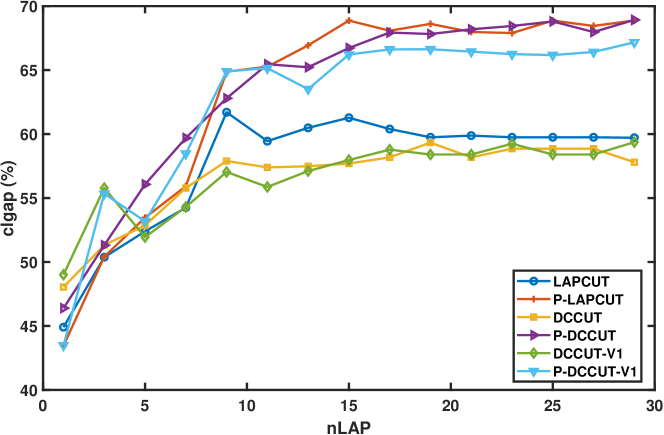
Figure 3: nLAP v.s. clgap for sample_30_0_10 using 6 cutting plane algorithms in $30$ seconds

Comments on numerical results in Figure 3 and Table 1

• The clgap is in general improved with the increase of nLAP, and the parallel algorithms always perform better than the algorithms without parallelism. The algorithms with best (i.e., maximal) clgap seem to be P-LAPCUT and P-DCCUT, then followed by P-DCCUT-V1, LAPCUT, DCCUT-V1 and DCCUT. The closed gap of all compared methods is obviously improved at the beginning of the increase of nLAP (which is not a surprise since more than one cut added in each iteration could improve the lower bound more quickly), then the best clgap is reached at some nLAP and barely improved for larger nLAP. The best choice for nLAP depends on the specific problems, the optimization methods and the computing resources. In general, if parallel computing resources are abundant enough, then the best nLAP could be found at the total number of integer variables (this test case is exactly an example). However, for large-scale integer optimization problems, setting nLAP to be the number of integer variables is generally impossible due to large number of variables, the limitation of resources and the cost of communications in parallel framework. In practice, for a given specific type of (MBLP), it is always suggested to try more CPUs until the clgap is barely improved or all available CPUs are fully utilized. Note that, constructing LAP cuts too quickly is not always good for lower bound improvement, as more LAP cuts require solving more linear programs and increase the size of the linear constraints thereafter, thus could slow down the improvement in clgap.

• P-DCCUT can always find the global optimal solution -83 within 30 seconds, while the other DCCUT type algorithms can often find global optimal solution as well. This interesting result is due to the use of DCA which allows to quickly find a global optimal solution even the gap and clgap are far from optimal. However, this will no longer be the case for LAPCUT type algorithms, since a global optimal solution can only be found when the gap is reduced to $0$ or the clgap is increased to 1. This observation demonstrates that DCCUT type algorithms have the advantage of quickly finding and updating good upper bound solutions.

5.2 Second Example: sample_10_0_10

The second example is a pure binary linear program with $10$ binary variables and $10$ linear constraints. The data is given by:

$$c^{\top}=\left[\begin{array}[]{cccccccccc}-2.2696&-0.3942&3.6018&-0.9882&-3.6844&2.9946&-0.6465&-0.4548&3.3601&-2.1507\end{array}\right],$$

$$A=\left[\begin{array}[]{cccccccccc}-0.9760&-0.2597&0.3479&-0.2245&-1.3819&-0.1699&1.8862&0.7490&-1.0811&-1.6861\\ -0.4179&-0.5955&-0.3371&-0.3062&0.8015&-1.4063&1.5717&-1.2475&-0.1122&1.4859\\ -0.7621&1.3052&0.5319&0.9497&1.6959&1.1078&0.6512&1.4769&-0.1982&-0.8773\\ -0.6498&0.0076&-0.3066&1.8852&1.1138&-0.7372&0.6152&-0.5799&-0.0836&-0.0105\\ 0.0810&-0.6236&-0.8002&0.8480&1.6002&-1.5630&-0.5826&0.9058&-1.2923&-1.5472\\ -1.0805&1.5700&1.0696&-0.0523&-0.5775&1.9393&0.7844&1.3766&-0.4787&0.6557\\ 1.9829&-0.0374&1.3243&1.4588&-1.8527&-0.7158&0.0847&1.4510&-0.5313&0.2882\\ -1.7562&1.8777&1.2762&-1.1542&1.4269&1.9436&-0.9917&1.8222&-0.2950&-1.4279\\ -0.5849&0.8489&-0.9042&0.8495&-0.6398&-1.2533&-0.5929&1.5026&-1.0576&-1.6837\\ -0.8693&1.5267&1.2275&-0.6247&0.9537&-0.8005&-1.2797&-0.3857&0.5152&0.0165\end{array}\right],$$

$$b^{\top}=\left[\begin{array}[]{cccccccccc}0.5288&0.7537&0.7413&0.1773&0.3005&0.2894&0.7848&0.2411&0.5476&0.2180\end{array}\right],$$

and the optimal value is 0.

We test $6$ cutting plane algorithms presented in subsection 5.1 for solving this problem. The absolute gap tolerance $\varepsilon$ is fixed to $0.01$ (i.e., algorithms will be terminated if $\texttt{UB}-\texttt{LB}\leq 0.01$). The updates of the UB (solid cycle line) and LB (dotted square line) with respect to the number of iterations are plotted in Figure 4. The numerical results are summarized in Table 2 where the best/worst computing time is highlighted in boldface/underline.

Table 2: Numerical results of different cutting plane algorithms (using up to 10 CPUs) for sample_10_0_10

Algorithms	nLAP	iter	LB	UB	gap(%)	clgap(%)	cut_dc1	cut_dc2	cut_lap	time(s)
DCCUT	1	27	1.478e-02	0	-1.46	100.22	1	13	40	1.156
P-DCCUT	10	9	4.795e-01	0	-32.41	107.17	1	4	86	0.833
DCCUT-V1	1	29	2.060e-01	0	-17.08	103.08	1	13	57	1.266
P-DCCUT-V1	10	9	3.220e-01	0	-24.36	104.82	1	4	99	1.127
LAPCUT	1	65	0	0	0.00	100.00	0	0	65	2.923
P-LAPCUT	10	16	0	0	0.00	100.00	0	0	83	1.356

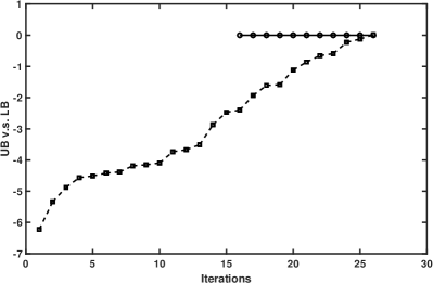
(a) DCCUT

(b) P-DCCUT

(c) DCCUT-V1

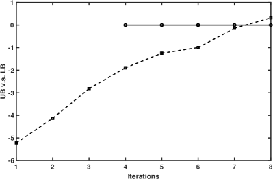
(d) P-DCCUT-V1

(e) LAPCUT

(f) P-LAPCUT

Figure 4: Updates of UB and LB in different cutting plane algorithms for sample_10_0_10

Comments on numerical results in Figure 4 and Table 2

• It is not surprise to see that the parallel algorithms always perform better than non-parallel ones. The fastest method is again P-DCCUT where $10$ CPUs are used for parallel workers. The slowest method is LAPCUT.

• The gap for DCCUT type algorithms could be negative, similar to the clgap which could be greater than $100\%$. This is due to the fact that the global optimal solution is found by DCA when gap and clgap are not optimal yet, then type-I DC cut (local cut) is introduced to cut off the global optimal solution, thus the lower bound on the reduced set could be greater than the current upper bound, which leads to negative gap and more than $100\%$ clgap. In both cases, the global optimality of the computed solution is guaranteed. Meanwhile, LAPCUT type algorithms can only have clgap between $0\%$ (initial) and $100\%$ (optimal), and the gap must be either $+\infty$ (non-optimal) or $0$ (optimal).

• Among non-parallel algorithms (DCCUT, DCCUT-V1 and LAPCUT), LAPCUT creates most number of LAP cuts, while DCCUT and DCCUT-V1 require less LAP cuts. This observation demonstrates the benefit of DC cuts which indeed accelerates the convergence of cutting plane algorithm by improving the lower bound more quickly than using LAP cuts alone.

• DCA is restarted in each iteration which not only helps to update upper bounds, but also leads to more DC cuts (type-I and type-II, cf. cut_dc1 and cut_dc2) for improving the lower bounds. It is worth noting that, once a global optimal solution is found by DCA, then restarting DCA in subsequent iterations will not improve UB anymore, but it is still helpful to construct DC cuts for LB improvement. However, as no one know the global optimality of the current UB, therefore, we cannot stop restarting DCA for UB updation until the convergence of the algorithm. In the case where UB is barely improved in many consecutive iterations, it is worth to think about reducing the probability of restarting DCA, which maybe useful to improve the overall performance of DCCUT type algorithms for solving hard cases.

5.3 Performance on MIPLIB 2017 dataset

Next, we will show some test results on the well-known benchmark testbed MIPLIB 2017 obtained from http://miplib.zib.de. We choose 14 problems in form of (MBLP) model whose information is given in Table 3. Note that all equality constraints $A_{eq}x+B_{eq}y=b_{eq}$ are converted into inequalities as $A_{eq}x+B_{eq}y\leq b_{eq}$ and $-A_{eq}x-B_{eq}y\geq-b_{eq}$. We are interested in the numerical results of clgap and gap for 6 cutting plane algorithms (namely, LAPCUT, P-LAPCUT, DCCUT, P-DCCUT, DCCUT-V1 and P-DCCUT-V1) tested within $120$ seconds and with fixed $\texttt{nLAP}=30$. The detailed numerical results are summarized in Table 4, where the algorithm provided the best clgap is highlighted in boldface.

Table 3: Tested problem information in MIPLIB 2017

Problem	Binary	Continuous	Constraints	$f^{0}$	fbest
neos5	53	10	63	13.00	15
mas74	150	1	13	10482.79528	11801.18572
mad	200	20	51	0	0.0268
pk1	55	31	45	0	11
assign1-5-8	130	26	161	183.36	212
ran14x18-disj-8	252	252	447	3444.42	3712
tr12-30	360	720	750	14210.43	130596
supportcase26	396	40	870	1288.102161	1745.123813
exp-1-500-5-5	250	740	550	28427.05	65887
neos-3754480-nidda	50	203	402	-1216923.27	12941.74
sp150x300d	300	300	450	4.89	69
mas76	150	1	12	38893.90364	40005.05399
neos-911970	840	48	107	23.26	54.76
gmu-35-40	1200	5	424	-2406943.556	-2406733.369

Table 4: Numerical results of different cutting plane algorithms (using up to 30 CPUs and $\texttt{nLAP}=30$) for MIPLIB benchmark within 120 seconds

Problem	LAPCUT	P-LAPCUT	DCCUT			P-DCCUT			DCCUT-V1			P-DCCUT-V1
	clgap(%)	clgap(%)	gap(%)	clgap(%)	UB	gap(%)	clgap(%)	UB	gap(%)	clgap(%)	UB	gap(%)	clgap(%)	UB
neos5	37.04	37.16	13.66	33.93	16.00	7.88	36.94	15.00	11.26	32.09	15.50	7.91	36.73	15.00
mas74	10.30	11.56	Inf	9.70	Inf	Inf	11.28	Inf	Inf	9.31	Inf	Inf	10.89	Inf
mad	0.00	0.00	44.35	0.00	0.80	43.08	0.00	0.76	44.35	0.00	0.80	47.81	0.00	0.92
pk1	0.00	0.00	96.30	0.00	26.00	95.00	0.00	19.00	96.30	0.00	26.00	93.75	0.00	15.00
assign1-5-8	18.79	21.12	Inf	16.81	Inf	12.82	19.85	217.00	Inf	16.79	Inf	Inf	19.96	Inf
ran14x18-disj-8	8.70	11.12	Inf	8.82	Inf	Inf	11.33	Inf	Inf	8.51	Inf	Inf	12.49	Inf
tr12-30	46.17	56.30	Inf	53.45	Inf	Inf	65.84	Inf	Inf	72.47	Inf	1.50	99.70	132228.00
supportcase26	24.26	27.44	Inf	26.91	Inf	Inf	30.51	Inf	Inf	22.79	Inf	Inf	28.49	Inf
exp-1-500-5-5	79.02	90.69	Inf	71.58	Inf	Inf	91.79	Inf	Inf	66.81	Inf	0.28	99.51	65887.00
neos-3754480-nidda	49.42	57.80	Inf	44.97	Inf	Inf	56.77	Inf	Inf	40.64	Inf	Inf	52.46	Inf
sp150x300d	75.05	100.00	Inf	62.59	Inf	Inf	98.44	Inf	Inf	65.18	Inf	0.00	100.00	69.00
mas76	9.28	11.71	Inf	9.42	Inf	Inf	11.11	Inf	Inf	8.25	Inf	Inf	10.73	Inf
neos-911970	82.74	91.68	62.64	83.40	134.24	42.65	91.32	91.46	62.64	83.40	134.24	29.68	91.69	74.57
gmu-35-40	0.00	0.02	Inf	0.03	Inf	Inf	0.05	Inf	Inf	0.00	Inf	Inf	0.06	Inf
Avg clgap	31.48	36.90	–	30.12	–	–	37.52	–		30.45	–	–	40.19	–

Comments on numerical results in Tables 4

• It is not surprising to see that the parallel algorithms outperform their non-parallel versions by improving the updation of lower bounds (i.e., with larger clgap). The best average clgap amounts to be P-DCCUT-V1, followed by P-DCCUT, P-LAPCUT, LAPCUT, DCCUT-V1 and DCCUT.

• It is interesting to see that the parallel DCCUT-V1 (P-DCCUT-V1) achieves the best average clgap, while the non-parallel version DCCUT-V1 gives the worst clgap in most of cases. This is probably due to the fact that P-DCCUT-V1 creates most cutting planes in each iteration, if these cuts can be processed in parallel, then the lower bound will be improved more quickly, which leads to the best clgap in P-DCCUT-V1; otherwise, it will take more time to create more cuts in each iteration for the non-parallel version, which leads to the worst performance in updating clgap within a limited time range.

• P-DCCUT-V1 obtains more upper bound solutions than the other algorithms. We think this should be caused by the best improvement of the lower bounds, which reduces quickly the search region and thus increases the probability for DCA to find feasible local solutions.

• Moreover, in some cases, e.g. tr12-30, P-DCCUT-V1 and P-DCCUT outperform P-LAPCUT which demonstrates again the benefit of DC cut.

Based on the above tests, we also believe that the introduction of DC cut as a type of user cut in GUROBI and CPLEX solvers should be helpful in improving the lower bounds and the overall performance of these solvers. DC cuts and the corresponding algorithms should be promising techniques for mixed binary programs, and deserve more attention in the community.

6 Conclusions and Perspectives

In this paper, we investigate the construction of two types of DC cuts (namely, dccut-type-I and dccut-type-II). The type-I DC cut is a local cut for feasible point, while the type-II DC cut is a global cut for fractional point. We discuss about the cases where DC cuts are constructable. Otherwise, we propose introducing classical global cuts, such as Lift-and-Project cut, Gomory’s mixed-integer cut and Mixed-integer rounding cut for instead. We give examples to illustrate the relationship between DC cuts with L&P cuts. Combining DC cuts and classical global cuts, we establish a cutting plane algorithm (cf. DCCUT algorithm) for solving problem (MBLP), whose convergence theorem is proved. A variant DCCUT algorithm (DCCUT-V1) by introducing more classical global cuts in each iteration, and parallel DCCUT algorithms are also proposed. Numerical results demonstrate that DCCUT type algorithms are able to find global optimal solution quickly without optimal gap or clgap, and DC cut can indeed improve the lower bound. By introducing parallelism, the performance of DCCUT algorithms are significantly improved, and P-DCCUT-V1 algorithm often outperforms the others with best clgap tested on some MBLP problems in the MIPLIB2017 dataset.

Some questions deserve more attention: (i) developing finite mixed integer programming DCCUT algorithm; (ii) How to guarantee, without knowing the set of vertices $V(\mathcal{K})$, that a given parameter $t$ is large enough for exact penalty and for type-II DC cut? (iii) proposing appropriate heuristic to restart DCA with a suitable probability for improving the overall performance of DCCUT type algorithms, especially to solve hard problems; (iv) introducing other classical cuts such as Gomory’s mixed-integer cuts, mixed-integer rounding cut, knapsack cut, cover cuts and clique cuts in DCCUT algorithm to improve again the lower bound; (v) extending DC cut from binary linear case to general integer nonlinear case.

Conflict of interest

The authors declare that they have no conflict of interest.

References

- (1) Achterberg, T.: Scip: solving constraint integer programs. Mathematical Programming Computation 1(1), 1–41 (2009)
- (2) Balas, E.: Intersection cuts – a new type of cutting planes for integer programming. Operations Research 19(1), 19–39 (1971)
- (3) Balas, E., Ceria, S., Cornuéjols, G.: A lift-and-project cutting plane algorithm for mixed 0–1 programs. Mathematical programming 58(1-3), 295–324 (1993)
- (4) Belotti, P., Lee, J., Liberti, L., Margot, F., Wächter, A.: Branching and bounds tighteningtechniques for non-convex minlp. Optimization Methods & Software 24(4-5), 597–634 (2009)
- (5) Benders, J.F.: Partitioning procedures for solving mixed-variables programming problems. Numerische mathematik 4(1), 238–252 (1962)
- (6) Bertsekas, D.P.: Nonlinear programming. Journal of the Operational Research Society 48(3), 334–334 (1997)
- (7) Bonami, P., Lee, J.: Bonmin user’s manual. Numer Math 4, 1–32 (2007)
- (8) Cornuéjols, G.: Valid inequalities for mixed integer linear programs. Mathematical Programming 112(1), 3–44 (2008)
- (9) Dantzig, G.B., Fulkerson, D.R., Johnson, S.M.: Solution of a large-scale traveling-salesman problem. Journal of the Operations Research Society of America 2(4), 393–410 (1954)
- (10) Dantzig, G.B., Fulkerson, D.R., Johnson, S.M.: On a linear-programming, combinatorial approach to the traveling-salesman problem. Operations Research 7(1), 58–66 (1959)
- (11) Efroymson, M., Ray, T.: A branch-bound algorithm for plant location. Operations Research 14(3), 361–368 (1966)
- (12) Gomory, R.: An algorithm for the mixed integer problem. Tech. rep., RAND CORP SANTA MONICA CA (1960)
- (13) Gomory, R.E., et al.: Outline of an algorithm for integer solutions to linear programs. Bulletin of the American Mathematical society 64(5), 275–278 (1958)
- (14) Gurobi: Gurobi 9.0.2. http://www.gurobi.com/
- (15) IBM: Ibm ilog cplex optimization studio v12.9.0 documentation
- (16) Jeroslow, R.G.: A cutting-plane game for facial disjunctive programs. SIAM Journal on Control and Optimization 18(3), 264–281 (1980)
- (17) Jörg, M.: k-disjunctive cuts and cutting plane algorithms for general mixed integer linear programs. Ph.D. thesis, Technische Universität München (2008)
- (18) Karp, R.M.: Reducibility among combinatorial problems. In: Complexity of computer computations, pp. 85–103. Springer (1972)
- (19) Kolesar, P.J.: A branch and bound algorithm for the knapsack problem. Management science 13(9), 723–735 (1967)
- (20) Le Thi, H.A., Moeini, M., Pham, D.T.: Portfolio selection under downside risk measures and cardinality constraints based on dc programming and dca. Computational Management Science 6(4), 459–475 (2009)
- (21) Le Thi, H.A., Nguyen, Q.T., Nguyen, H.T., Pham, D.T.: Solving the earliness tardiness scheduling problem by dc programming and dca. Mathematica Balkanica 23(3-4), 271–288 (2009)
- (22) Le Thi, H.A., Pham, D.T.: A continuous approach for large-scale constrained quadratic zero-one programming. Optimization 45(3), 1–28 (2001)
- (23) Le Thi, H.A., Pham, D.T.: A continuous approch for globally solving linearly constrained quadratic zero-one programming problems. Optimization 50(1-2), 93–120 (2001)
- (24) Le Thi, H.A., Pham, D.T.: The dc (difference of convex functions) programming and dca revisited with dc models of real world nonconvex optimization problems. Annals of Operations Research 133(1-3), 23–46 (2005)
- (25) Le Thi, H.A., Pham, D.T.: Dc programming and dca: thirty years of developments. Mathematical Programming 169(1), 5–68 (2018)
- (26) Le Thi, H.A., Pham, D.T., Le Dung, M.: Exact penalty in dc programming. Vietnam J. Math. 27(4), 169–178 (1999)
- (27) Le Thi, H.A., Pham, D.T., Van Ngai, H.: Exact penalty and error bounds in dc programming. Journal of Global Optimization 52(3), 509–535 (2012)
- (28) Marchand, H., Martin, A., Weismantel, R., Wolsey, L.: Cutting planes in integer and mixed integer programming. Discrete Applied Mathematics 123(1-3), 397–446 (2002)
- (29) MathWorks: Matlab documentation. http://www.mathworks.com/help/matlab/
- (30) Mosek, A.: The mosek optimization software. http://www.mosek.com
- (31) Ndiaye, B.M., Pham, D.T., Niu, Y.S., et al.: Dc programming and dca for large-scale two-dimensional packing problems. In: Asian Conference on Intelligent Information and Database Systems, pp. 321–330. Springer (2012)
- (32) Nguyen, V.V.: Méthodes exactes pour l’optimisation dc polyédrale en variables mixtes 0-1 basées sur dca et des nouvelles coupes. Ph.D. thesis, INSA-Rouen (2006)
- (33) Niu, Y.S.: Programmation dc et dca en optimisation combinatoire et optimisation polynomiale via les techniques de sdp: codes et simulations numériques. Ph.D. thesis, INSA-Rouen (2010)
- (34) Niu, Y.S.: On combination of dca, branch-and-bound and dc cut for solving mixed 0-1 linear program. In: 21st International Symposium on Mathematical Programming (ISMP2012). Berlin (2012)
- (35) Niu, Y.S.: Pdcabb: A parallel mixed-integer nonlinear optimization solver (parallel dca-bb global optimization algorithm). https://github.com/niuyishuai/PDCABB (2017)
- (36) Niu, Y.S.: A parallel branch and bound with dc algorithm for mixed integer optimization. In: The 23rd International Symposium in Mathematical Programming (ISMP2018), Bordeaux, France (2018)
- (37) Niu, Y.S., Glowinski, R.: Discrete dynamical system approaches for boolean polynomial optimization. Preprint arXiv:1912.10221 (2019)
- (38) Niu, Y.S., Pham, D.T.: A dc programming approach for mixed-integer linear programs. In: International Conference on Modelling, Computation and Optimization in Information Systems and Management Sciences, pp. 244–253. Springer (2008)
- (39) Niu, Y.S., Pham, D.T.: Efficient dc programming approaches for mixed-integer quadratic convex programs. In: Proceedings of the International Conference on Industrial Engineering and Systems Management (IESM2011), pp. 222–231 (2011)
- (40) Niu, Y.S., Pham, D.T.: Dc programming approaches for bmi and qmi feasibility problems. In: Advanced Computational Methods for Knowledge Engineering, pp. 37–63. Springer (2014)
- (41) Niu, Y.S., You, Y., Xu, W., Ding, W., Hu, J., Yao, S.: A difference-of-convex programming approach with parallel branch-and-bound for sentence compression via a hybrid extractive model. Optimization Letters pp. 1–26 (2021)
- (42) Pang, J.S., Razaviyayn, M., Alvarado, A.: Computing b-stationary points of nonsmooth dc programs. Mathematics of Operations Research 42(1), 95–118 (2017)
- (43) Pham, D.T., Bouvry, P., et al.: Solving the perceptron problem by deterministic optimization approach based on dc programming and dca. In: 7th IEEE International Conference on Industrial Informatics, pp. 222–226. IEEE (2009)
- (44) Pham, D.T., Le Thi, H.A.: Convex analysis approach to dc programming: theory, algorithms and applications. Acta mathematica vietnamica 22(1), 289–355 (1997)
- (45) Pham, D.T., Le Thi, H.A.: A dc optimization algorithm for solving the trust-region subproblem. SIAM Journal on Optimization 8(2), 476–505 (1998)
- (46) Pham, D.T., Le Thi, H.A., Pham, V.N., Niu, Y.S.: Dc programming approaches for discrete portfolio optimization under concave transaction costs. Optimization letters 10(2), 261–282 (2016)
- (47) Quang, T.N.: Approches locales et globales basées sur la programmation dc et dca pour des problèmes combinatoires en variables mixtes 0-1: applications à la planification opérationnelle. Ph.D. thesis, Université Paul Verlaine-Metz (2010)
- (48) Robinson, J.: On the hamiltonian game (a traveling salesman problem). Rand Corporation (1949)
- (49) Sahinidis, N.V.: Baron: A general purpose global optimization software package. Journal of global optimization 8(2), 201–205 (1996)
- (50) Schleich, J., Le Thi, H.A., Bouvry, P.: Solving the minimum m-dominating set problem by a continuous optimization approach based on dc programming and dca. Journal of combinatorial optimization 24(4), 397–412 (2012)