FedPower: Privacy-Preserving Distributed Eigenspace Estimation 

Abstract

Eigenspace estimation is fundamental in machine learning and statistics, which has found applications in PCA, dimension reduction, and clustering, among others. The modern machine learning community usually assumes that data come from and belong to different organizations. The low communication power and the possible privacy breaches of data make the computation of eigenspace challenging. To address these challenges, we propose a class of algorithms called FedPower within the federated learning (FL) framework. FedPower leverages the well-known power method by alternating multiple local power iterations and a global aggregation step, thus improving communication efficiency. In the aggregation, we propose to weight each local eigenvector matrix with Orthogonal Procrustes Transformation (OPT) for better alignment. To ensure strong privacy protection, we add Gaussian noise in each iteration by adopting the notion of differential privacy (DP). We provide convergence bounds for FedPower that are composed of different interpretable terms corresponding to the effects of Gaussian noise, parallelization, and random sampling of local machines. Additionally, we conduct experiments to demonstrate the effectiveness of our proposed algorithms.

Keywords: Communication Efficiency, Federated Learning, Power Method, Stragglers’ Effect

1 Introduction

Modern machine learning tasks involve massive data that come from different sources, such as hospitals, banks, companies, etc. The communication power is thus limited, which makes large-scale data applications challenging. Further, the data from local sources often contain sensitive information about individuals, hence, privacy issues become more and more prominent (Bhowmick et al., 2018; Dwork et al., 2014a).

Federated learning (FL) has emerged as a prominent paradigm for distributed learning in large-scale problems involving multi-source data. For further background and recent advancements, please refer to Kairouz et al. (2021) and related literature. In FL, each machine typically trains its model locally and sends parameter updates to the central server whenever communication is required. The server then aggregates these updates, potentially with randomization, and broadcasts them to synchronize all local parameters. This process is iterated until convergence or the fulfillment of specific conditions. To address the aforementioned challenges including large-scale data and unreliable communication, autonomy, and privacy issues; see McMahan et al. (2017); Smith et al. (2017); Sattler et al. (2019); li2020challenges, a good FL algorithm should meet the following requirements. First, a FL algorithm should be communication efficient with more local computations and fewer communications. Second, it should be able to deal with the scheme when some of the local machines are inactive or the organizations decide not to participate in the following training procedures. Third, individual’s privacy should be protected, which is ensured apparently by leaving the original data at local machines.

Nevertheless, even if only the updates but not the original data are transmitted to the central server, individuals’ privacy can still be compromised through via delicately designed attacks (Dwork et al., 2017; Melis et al., 2018; Zhou and Tang, 2020). To address this issue, the framework of differential privacy (DP) (Dwork et al., 2006, 2014a) has gained widespread attention in private data analysis. A differentially private (DP) algorithm pursues that if the data is changed by one row (entry) with pre-specified limits, then the algorithm’s output appears similar in probability. Such algorithms protect the individuals’ privacy from any adversary who knows the algorithm’s output and even the rest of the data and can resist any kind of attack. Typically, a differentially private algorithm is obtained by adding calibrated noise to the non-differentially private algorithm.

This paper focuses on the problem of eigenspace estimation within the private-preserving federated learning framework. Eigen-decomposition is a widely used technique in various machine learning tasks, such as dimension reduction (Wold et al., 1987), clustering (Von Luxburg, 2007), ranking (Negahban et al., 2017), matrix completion (Candès and Recht, 2009), multiple testing (Fan et al., 2019a), and factor analysis (Bai and Ng, 2013). It also finds applications in fields like finance, biology, and neurosciences (Izenman, 2008). The computation of eigenvectors has evolved since the 1960s, with seminal works by Golub and Kahan (1965); Golub and Reinsch (1970) that provided the basis for the EISPACK and LAPACK routines. For computing leading eigenspace of matrices, iterative algorithms such as the power iteration and its variants (Golub and Van Loan, 2012; Hardt and Price, 2014) flourished. Recently, to solve large-scale problems, distributed learning of eigenvectors or principle components is receiving more and more attention; see Fan et al. (2019b); Chen et al. (2021), among others. However, as far as we are aware, most existing works can not meet the aforementioned challenges simultaneously.

To tackle the challenges of large-scale computation, unreliable communication, and privacy breaches in modern data analysis, we propose a set of algorithms called the Federated Power method (FedPower). Building upon the well-known single-machine power method, FedPower assumes a distributed data setting, where each machine performs local power iterations using its data. After several local steps, the local machines send their updates to the central server, which aggregates and returns the results back to the machines. Due to the orthogonal ambiguity of subspaces, we employ the Orthogonal Procrustes Transformation (OPT) during the aggregation. As connectivity issues may occur during the training process where each local machine may lose connection to the server actively or passively, we present two protocols: full participation and partial participation. In the partial participation protocol, the server may collect the first few responded local machines within a certain time range. We model this by assuming that the local machines are sampled with the replacement for fixed times. Moreover, to avoid privacy leakage, we take advantage of the notion of DP to add Gaussian noise to the updates in each iteration. This is based on our assumption that the server is honest-but-curious (semi-honest).

In addition to the algorithms, we study how the FedPower performs theoretically. Firstly, we provide rigorous analysis demonstrating the DP guarantees of the algorithms corresponding to both the full and partial participation schemes. These guarantees are established using the notion of Rényi differential privacy (Mironov, 2017). Secondly, we analyze the convergence bound of FedPower in terms of the subspace distance between the estimated and the true eigenspace using advanced random matrix theory and delicate error decomposition techniques. For the full participation scheme, the convergence error comprises two components. One component arises from the Gaussian noise, while the other comes from the parallelization and synchronization. For the partial participation scheme, the resulting convergence error bound consists of three components. Besides the two components appearing in the error of the full participation scheme, there exists an additional component that comes from the sampling of local machines, which could be regarded as the sampling bias term. The more local machines that are sampled, the smaller the bias term would be. As expected, the final error bounds can be made sufficiently small by ensuring a sufficiently large-sample and high-quality local data.

The remainder of the paper is organized as follows. Section 2 introduces the power method for the centralized and distributed eigenspace estimation, and two notions of DP. Section 3 includes the proposed algorithms FedPower and the corresponding convergence analysis under two schemes, namely, the full participation and the partial participation. Section 4 reviews and discusses the related works, and also summarizes the main contributions of this work. Section 5 presents the experimental results. Section 6 concludes the paper. Technical proofs and supplementary materials are all included in the Appendix.

2 Preliminaries

In this section, we first present the power method for computing the eigenspace, and a naive distributed power method designed for the distributed eigenspace computation. Then, we pose the demand, namely, the communication efficiency and privacy preservation, that the modern machine learning tasks call for. In particular, we propose one adversary model to show how privacy can be leaked during the communication rounds of the naive distributed power method. Last, we present the preliminaries of $(\epsilon,\delta)$-DP and its variant Rényi differential privacy.

2.1 Eigen-decomposition and Power Method

Given a positive semi-definite matrix $A\in\mathbb{R}^{d\times d}$, its full eigen-decomposition is defined as

$${A=U{\Sigma}U^{\intercal}=\sum_{i=1}^{d}{\sigma_{i}}u_{i}u_{i}^{\intercal},}$$

where $U=[u_{1},u_{2},\dots,u_{d}]\in\mathbb{R}^{d\times d}$ are orthogonal matrices that contain the eigenvectors of $A$, and $\Sigma={\rm diag}\{\sigma_{1},\sigma_{2},\ldots,\sigma_{d}\}$ is a diagonal matrix with the eigenvalues in decreasing order on the diagonal. The partial or truncated eigen-decomposition aims to compute the top $k~{}(k\leq d)$ eigenvectors $U_{k}=[u_{1},\ldots,u_{k}]$ and use the truncated decomposition $U_{k}\Sigma_{k}U_{k}^{\intercal}$ to approximate $A$, where $\Sigma_{k}={\rm diag}\{\sigma_{1},\ldots,\sigma_{k}\}$.

The power method (Golub and Van Loan, 2012) computes $U_{k}$ by iterating

$$Y\leftarrow AZ\quad{\rm and}\quad Z\leftarrow{\rm\textsf{orth}}(Y),$$ (2.1)

where $Y$ and $Z$ are $d\times k$ matrices, and ${\rm\textsf{orth}}(Y)$ means orthogonalizing the columns of $Y$ via QR-factorization.

2.2 Distributed Power Method

Suppose $A$ is stored at $m$ different local machines such that

$$A=\frac{1}{m}\sum_{i=1}^{m}A_{i}.$$ (2.2)

Typically, we consider the scenario where $A=\frac{1}{n}M^{\intercal}M$ for some $M\in\mathbb{R}^{n\times d}$. Suppose that $M$ is partitioned to $m$ blocks by row such that $M^{\intercal}=[M_{1}^{\intercal},...,M_{m}^{\intercal}]$, where $M_{i}\in\mathbb{R}^{s_{i}\times d}$ includes $s_{i}$ rows of $M$ and $\sum_{i=1}^{m}s_{i}=n$. For simplicity, we assume that $M$ is equally partitioned and $s_{i}=\frac{n}{m}$ for all $i$’s, yet we note that the results can be easily extended to more general cases. It is then clear that

$$A_{i}=\frac{m}{n}M_{i}^{\intercal}M_{i}.$$ (2.3)

For notational simplicity, we refer $A_{i}$ in what follows but one should keep (2.3) in mind.

With (2.2), $Y$ in (2.1) can be written as

$$Y=\frac{1}{m}\sum_{i=1}^{m}A_{i}Z\in\mathbb{R}^{d\times k},$$

which implies that the power method can be parallelized. See Figure 1 and Algorithm 1, which is called the distributed power method. Note that Algorithm 1 is identical to the power method except that the summations therein come from different workers. The following theorem is a well-known result on the convergence of the power method as well as the distributed power method (Arbenz, 2012).

Theorem 1.

Let $\sigma_{k}$ be the $k$-th largest eigenvalue of $A$ and assume $\sigma_{k+1}>0$, where $1\leq k<d$. Then for any $\epsilon>0$, with high probability, after $T=O(\frac{\sigma_{k}}{\sigma_{k+1}}{\rm log}(\frac{d}{\epsilon}))$ iterations, the output ${Z}_{T}$ of Algorithm 1 satisfies

$${\rm sin}\theta_{k}({Z}_{T},U_{k})=\|(\mathbb{I}_{d}-{Z}_{T}{Z}_{T}^{\intercal})U_{k}\|_{2}\leq\epsilon,$$

where ${\rm sin}\theta_{k}$ denotes the $k$-th principle angles between two subspaces which can be regarded as a subspace distance , and $\mathbb{I}_{d}$ denotes the identity matrix of dimension $d$.

The distributed power method can deal with data distributed across multiple workers. However, it falls short of addressing the challenges and concerns encountered in modern data applications. Firstly, Algorithm 1 necessitates two communication rounds in each iteration, resulting in substantial communication costs when simple parallelizing the power method. Furthermore, the issues of the straggler’s effect and privacy breaches are yet to be resolved. In the subsequent subsections, we will delve into further explanations of these two concerns.

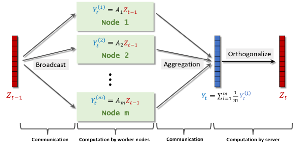
Figure 1: Protocol of the distributed power method. In every iteration, there are two rounds of communications.

Algorithm 1 Distributed Power Method

1:  Input: distributed dataset $\{A_{i}\}_{i=1}^{m}$, target rank $k$, number of iterations $T$.

2:  Initialization: orthonormal $Z_{0}^{(i)}=Z_{0}\in\mathbb{R}^{d\times k}$ by QR decomposition on a random Gaussian matrix with i.i.d. entries from $\mathcal{N}(0,1)$.

3:  for $t=1$ to $T$ do

4:     The $i$-th worker independently performs $Y_{t}^{(i)}=A_{i}Z_{t-1}^{(i)}$ for all $i\in[m]$;

5:     Each worker $i$ sends $Y_{t}^{(i)}$ to the server and the server performs aggregation: $Y_{t}=\sum_{i=1}^{m}\frac{1}{m}Y_{t}^{(i)}$;

6:     The server performs orthogonalization: $Z_{t}={\rm\textsf{orth}}(Y_{t})$ and broadcast $Z_{t}$ to each worker such that $Z_{t}^{(i)}=Z_{t}$;

7:  end for

8:  Output: approximated eigen-space ${Z}_{T}\in\mathbb{R}^{d\times k}$ with orthonormal columns.

2.3 Straggler’s Effect

Unlike traditional distributed learning, the FL system operates under the premise that the server does not have control over the local machines, leading to potential disconnections between the server and the local machines (Kairouz et al., 2021; Li et al., 2020b). This introduces two key considerations. Firstly, certain local machines may experience issues such as being powered off, encountering technical failures, or having limited internet connectivity, thereby becoming stragglers. Secondly, each local machine retains its autonomy, with the owners having the discretion to opt out of specific training steps for various reasons. Consequently, waiting for responses from all local machines becomes unfeasible for the server. Instead, the server can utilize the updates from the first few responsive local machines within a predetermined timeframe. Our proposed algorithm effectively captures and accounts for the impact of stragglers.

2.4 Adversary Model

Though the data are not shared by all the participants in FL or more general distributed learning systems, privacy breaches remain possible. In this paper, we consider a specific adversary termed as the curious onlooker, who can eavesdrop on the communication between the server and the local machines and possesses knowledge of the learning tasks and protocols. We consider the server as a potential onlooker, characterized as honest-but-curious (semi-honest). This means that while the server does not violate the protocol to attack the raw data, it is curious and will attempt to learn all possible information from its received messages (Goldreich, 2009). For instance, in a company, internal employees responsible for model training may attempt to infer personal information about the users. Additionally, we assume that each local machine is honest and does not attempt to infer information from other machines. The following example demonstrates how the distributed power method (Algorithm 1) can potentially cause privacy threats to curious onlookers.

Example 1 (Privacy breaches via curious onlookers).

Consider Algorithm 1 and assume that the server knows the updates $Y_{t}^{(i)}$ for each $i\in[m]$ and $t\in T$. In addition, the server could infer $Z_{t}^{(i)}$ from $Y_{t}^{(i)}$ because it also knows the learning rule that $Z_{t}^{(i)}$ is obtained from $Y_{t}^{(i)}$ via the QR decomposition (Line 6 in Algorithm 1). Then by

$$Y_{t}^{(i)}=A_{i}Z_{t-1}^{(i)}\;{\mbox{(Line 4 in Algorithm \ref{dispower})}},$$ (2.4)

and the results in Theorem 1 that the distributed power method converges after $T=O(\frac{\sigma_{k}}{\sigma_{k+1}}{\rm log}(\frac{d}{\epsilon}))$ iterations, the server can infer $A_{i}$ using $d\times k\times T$ equations provided that there are at most $O(d\log d)$ unknown elements in $A_{i}$. Indeed, the server may participate in the data collection, therefore they may know some prior information about $A_{i}$.

We have presented a simple example to illustrate the potential privacy leakage that can occur through curious onlookers. It is important to note that more sophisticated attacks can be found in studies such as Madry et al. (2017); Chakraborty et al. (2018), among others.

2.5 Differential Privacy

We have seen that privacy concerns are prevailing in modern data analysis. How to quantitatively describe privacy is the key point to understanding and designing privacy-preserving algorithms. Differential privacy, first introduced in Dwork et al. (2006), is a rigorous and most widely adopted notion of privacy, which generally guarantees that a randomized algorithm behaves similarly on similar input databases. The $(\varepsilon,\delta)$-DP (Dwork et al., 2014a) is defined as follows. Throughout this paper, we use the term "DP" as an abbreviation for “differential privacy” or “differentially private”, following common usage in the field.

Definition 1 ($(\varepsilon,\delta)$-DP).

A randomized algorithm $\mathcal{M}$: $\mathcal{X}^{n}\rightarrow\Theta$ is called $(\varepsilon,\delta)$-DP if for all pairs of neighboring databases $X,X^{\prime}\in\mathcal{X}^{n}$, and for all subsets of range $S\subseteq\Theta$:

$$\mathbb{P}(\mathcal{M}(X)\in S)\leq{\rm exp}(\varepsilon)\mathbb{P}(\mathcal{M}(X^{\prime})\in S)+\delta.$$

In literature, the definition of neighboring datasets $X,X^{\prime}$ varies case by case. In this work, dataset $X$ is the data matrix $M_{i}$ introduced in Section 2.2, and we consider the scenario where “neighboring” means $M_{i}$ and $M^{\prime}_{i}$ differ in one row, with a Euclidean norm of 1. DP achieves the privacy goal that anything can be learned about an individual from the released information can also be learned without that individual’s participation. The $\varepsilon$ is often called the privacy budget which is a small constant measuring the privacy loss and it should be no larger than 1 typically (Dwork et al., 2014a). The $\delta$ is also a small constant and it can be thought of as a tolerance of the more stringent $\varepsilon$-DP, i.e., $(\varepsilon,\delta)$-DP with $\delta$ being 0.

While $(\varepsilon,\delta)$-DP is interpretable and user-friendly, it can not tightly handle composition, that is, how much the privacy loss accumulates under repeated quires on the same data. To ensure the exact composition, many new notions of DP have been developed, such as concentrated differential privacy (Dwork and Rothblum, 2016), Rényi differential privacy (Mironov, 2017), truncated concentrated differential privacy (Bun et al., 2018), and Gaussian differential privacy (Dong et al., 2019), among others. In this work, we specifically focus on Rényi differential privacy (RDP).

Definition 2 ($(\alpha,\varepsilon)$-RDP).

A randomized algorithm $\mathcal{M}$: $\mathcal{X}^{n}\rightarrow\Theta$ is called $\epsilon$-Rényi DP of order $\alpha$, or $(\alpha,\varepsilon)$-RDP, if for all pairs of neighboring databases $X,X^{\prime}\in\mathcal{X}^{n}$,

$$D_{\alpha}(\mathcal{M}(X)\|\mathcal{M}(X^{\prime})):=\frac{1}{\alpha-1}\log\mathbb{E}_{x\sim\mathcal{M}(X^{\prime})}\left[\left(\frac{\mathcal{M}(X)(x)}{\mathcal{M}(X^{\prime})(x)}\right)^{\alpha}\right]\leq\varepsilon.$$

RDP can be achieved using the following Gaussian mechanism (Mironov, 2017).

Proposition 2 (RDP Gaussian mechanism).

For any $f:\mathcal{X}^{n}\rightarrow\mathbb{R}^{d}$, its $l_{2}$-sensitivity is defined by

$$\triangle_{2}(f)=\underset{X,X^{\prime}\,\mbox{\tiny neighboring}}{\sup}\|f(X)-f(X^{\prime})\|_{2}.$$

If ${\triangle_{2}(f)<\Delta}$, then the Gaussian mechanism given by

$$\mathcal{M}(X):=f(X)+(\xi_{1},\xi_{2},\dots,\xi_{d})^{\intercal},$$

where the $\xi_{i}$ are i.i.d.  drawn from $\mathcal{N}(0,\nu^{2})$, achieves $(\alpha,\frac{\alpha\Delta^{2}}{2\nu^{2}})$-RDP for any $\alpha>1$.

RDP enjoys the following two nice properties (Mironov, 2017). One is the composition property, that is, the privacy degrade of repeated mechanisms is just the summation of the privacy budgets of each mechanism. The other is the post-processing property, meaning that an $(\alpha,\varepsilon)$-RDP algorithm is still $(\alpha,\varepsilon)$-RDP after any post-processing procedure provided that no additional knowledge about the database is used.

Proposition 3 (Adaptive composition of RDP).

For $\alpha\in(1,\infty)$, suppose $\mathcal{M}_{1}:\mathcal{X}^{n}\rightarrow\Theta_{1}$ is $(\alpha,\varepsilon_{1})$-RDP and $\mathcal{M}_{2}:\mathcal{X}^{n}\times\Theta_{1}\rightarrow\Theta_{2}$ is $(\alpha,\varepsilon_{2})$-RDP, which takes as input the output of the first mechanism $\mathcal{M}_{1}$ in addition to the dataset. Then, the joint mechanism $\mathcal{M}:\mathcal{X}^{n}\rightarrow\Theta_{1}\times\Theta_{2}$ defined as

$$\mathcal{M}(X)=(\theta_{1},\mathcal{M}_{2}(X,\theta_{1}))$$

achieves $(\alpha,\varepsilon_{1}+\varepsilon_{2})$-RDP, where $X\subset\mathcal{X}^{n}$ and $\theta_{1}=\mathcal{M}_{1}(X)$.

The composition of RDP can be generalized to multiple compositions.

Proposition 4 (Post-processing of RDP).

Let $\mathcal{M}:\mathcal{X}^{n}\rightarrow\Theta$ be an $(\alpha,\varepsilon)$-RDP algorithm, and $g:\Theta\rightarrow\Theta^{\prime}$ be an arbitrary randomized mapping. Then $g\circ\mathcal{M}:\mathcal{X}^{n}\rightarrow\Theta^{\prime}$ is $(\alpha,\varepsilon)$-RDP.

We also have the conversion of RDP to $(\varepsilon,\delta)$-DP to enhance the interpretability of DP.

Proposition 5 (RDP to DP).

If $\mathcal{M}$ is $(\alpha,\varepsilon)$-RDP, then $\mathcal{M}$ is $(\varepsilon+\frac{\log(1/\delta)}{\alpha-1},\delta)$-DP for $\forall 0<\delta<1$.

All the properties enhance the utility of RDP in practical applications.

2.6 Notation

We summarize the notation and notions used in the following sections of this paper. Given a target matrix $A\in\mathbb{R}^{d{\times}d}$, the $k$-th largest eigenvalue of $A$ is denoted by $\sigma_{k}$. Let $k$ and $r\ (r\geq k)$ be the target rank and iteration rank of partial eigen-decomposition, respectively. The numbers of total iterations is denoted by $T$ and the set $\{1,\ldots,T\}$ is denoted by $[T]$. $\|\cdot\|_{2}$ denotes the spectral norm of a matrix or the Euclidean norm of a vector, $\|\cdot\|_{\tiny{\rm max}}$ denotes the entry-wise maximum absolute value of a matrix or a vector, $\|\cdot\|_{\infty}$ denotes the matrix operator $\ell_{\infty}$ norm, and $\|\cdot\|_{\tiny{\rm m}}$ denotes the minimum singular value of a matrix. Let $\kappa=\|A\|_{2}\|A^{\dagger}\|_{2}$ denote target matrix $A$’s condition number. $\mathcal{O}_{r}$ denotes the set of $r\times r$ orthogonal matrices and $\mathbb{I}_{r}$ denotes the identity matrix with dimension $r$.

In addition, we use the following standard notation for asymptotics. We write $f(n)\asymp g(n)$ if $cg(n)\leq f(n)\leq Cg(n)$ for some constants $0<c<C<\infty$. $f(n)\lesssim g(n)$ or $f(n)=O(g(n))$ if $f(n)\leq Cg(n)$ for some constant $C<\infty$. $f(n)=\Omega(g(n))$ if $f(n)\geq cg(n)$ for some constant $c>0$. Finally, we provide the definition of projection distance, which measures the distance of two subspaces.

Definition 3 (Projection distance).

Given two column-orthonormal matrices $U,\tilde{U}\in\mathbb{R}^{d\times k}$, the projection distance between the two subspaces spanned by their columns is defined as

$${\rm dist}(U,\tilde{U}):=\|UU^{\intercal}-\tilde{U}\tilde{U}^{\intercal}\|_{2}=\|\tilde{U}^{\intercal}U^{\bot}\|_{2}=\|{U}^{\intercal}\tilde{U}^{\bot}\|_{2}={\rm sin}\,\theta_{k}(U,\tilde{U}),$$ (2.6)

where $U^{\bot}$ and $\tilde{U}^{\bot}$ denote the complement subspaces of $U$ and $\tilde{U}$, respectively. Here $\theta_{k}$ denotes the $k$-th principle angle between two subspaces; see Appendix E for the formal definition.

3 Privacy-Preserving Distributed Eigenspace Estimation

In this section, we develop a set of power-iteration-based algorithms, called FedPower, for the eigenvector computation which is communication efficient, privacy-preserving, and allows for partial participation of the local machines. In particular, depending on whether the local machines all participate in the communication rounds, we study two protocols, namely, the full participation protocol and the partial participation protocol. The privacy bounds and convergence rates will also be established.

Before delving into the details, let us provide an overview of the basic idea behind FedPower, as depicted in Figure 2. The setup is consistent with that described in Section 2.2. To improve the communication efficiency of the naive distributed power method, FedPower trades more local computations for fewer communications. Specifically, each worker locally runs

$$Y_{t}^{(i)}=A_{i}Z_{t-1}^{(i)}$$

multiple times between two communication rounds. Let $T$ be the total number of iterations performed by each worker. Let $\mathcal{I}_{T}$, a subset of $[T]$, index the iterations that call for communications. $|\mathcal{I}_{T}|$ denotes its cardinality. If $\mathcal{I}_{T}=[T]$, synchronization happens at every iteration as in the distributed power method (see Figure 1). If $\mathcal{I}_{T}=\{T\}$, synchronization happens only at the end, and FedPower is similar to the one-shot divide-and-conquer eigenspace (Fan et al., 2019b). An important example that we will focus on latter is $\mathcal{I}_{T}^{p}$. It is defined by

$$\mathcal{I}_{T}^{p}=\{t\in[T]:t\ \text{mod}\ p=0\}=\{0,p,2p,\cdots,p\lfloor T/p\rfloor\},$$ (3.1)

where $p$ is a positive integer and $\lfloor T/p\rfloor$ is the largest integer which is smaller than $T/p$. FedPower with $\mathcal{I}_{T}^{p}$ only performs communications every $p$ iterations.

In order to address the orthogonal ambiguity of subspaces, the central server performs an average of the orthogonally transformed local eigenvectors during communication, denoted as $Y_{t}^{(i)}D_{t}^{(i)}$, instead of using the raw $Y_{t}^{(i)}$ values. The orthogonal matrices $D_{t}^{(i)}$ are constructed using the following procedure. First, we choose a baseline local machine that to be aligned with. Without loss of generality, we assume the first machine is chosen in the following paper. Next, we compute

$$D_{t}^{(i)}=\underset{D\in\mathcal{F}\cap\mathcal{O}_{r}}{{\rm argmin}}\;\|Z_{t-1}^{(i)}D-Z_{t-1}^{(1)}\|_{F},$$ (3.2)

where $\mathcal{O}_{r}(r\geq k)$ denotes the set of $r\times r$ orthogonal matrices. The choice of $\mathcal{F}$ can vary depending on the specific scenario. When $\mathcal{F}=\{\mathbb{I}_{r}\}$, the feasible set contains a single element, and as a result, $D_{t}^{(i)}=\mathbb{I}_{r}$. When $\mathcal{F}=\mathcal{O}_{r}$, (3.2) represents the classical matrix approximation problem known as the Procrustes problem (Schönemann, 1966; Cape, 2020). The solution to (3.2), referred to as the Orthogonal Procrustes Transformation (OPT), can be obtained in closed form:

$$D_{t}^{(i)}\;=\;W_{1}W_{2}^{\intercal},$$

where we assume that the SVD of $(Z^{(i)}_{t-1})^{\intercal}Z^{(1)}_{t-1}$ is $W_{1}\Lambda W_{2}^{\intercal}$. The concurrent work (Charisopoulos et al., 2021) also uses OPT.

Recall that we consider a strong adversary termed as honest-but-curious onlooker (see Section 2.4) who does not violate the rules to peep the raw data but is curious to infer data information from the communicative messages and the training rule. To prevent the potential privacy breaches, we consider the record-level DP that protects each row of one device’s data $M_{i}$’s which has Euclidean norm 1; recall also (2.3). We note that the client-level DP that protects against the whole data of each device has also been studied in FL (McMahan et al., 2018). However, this kind of privacy guarantee is too strong if the devices represent different organizations, say hospitals, companies, banks, etc (Li et al., 2019a; Zheng et al., 2021). In the record-level DP’s, we add calibrated Gaussian noise after each local steps on each active devices. After tight composition analysis of DP, the procedure can be shown to be DP at given privacy budget.

Finally, to take into account the straggler’s effect, we also consider the partial participation protocol, that is, each aggregation only involves the first $K$ responded (not necessarily different) machines before a certain time. Specifically, we model such a setting using sampling with replacement strategy.

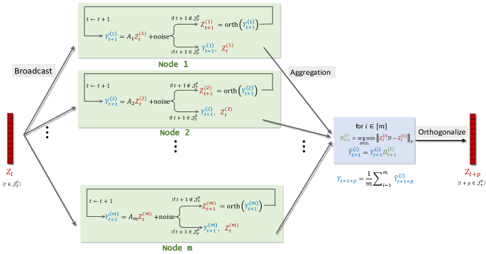
Figure 2: The full participation protocol of FedPower involves each local machine conducting noisy power iterations locally until a communication step is triggered. When communication occurs ($t+1\in\mathcal{I}_{T}^{p}$), the local machines transmit the updates $Y_{t+1}^{(i)}$ and previous $Z_{t}^{(i)}$ to the server. Subsequently, the server performs alignment and aggregation procedures.

3.1 Federated Power Method under Full Participation Protocol

The FedPower under the full participation protocol is shown in Algorithm 2, where we allow the iteration rank $r$ (i.e., the dimension of the output) being equal or larger than the target rank $k$, and we use $\mathcal{N}(0,\nu^{2})^{d\times r}$ to denote a $d\times r$ random matrix with each entry being i.i.d. $\mathcal{N}(0,\nu^{2})$. We have the following remark on Algorithm 2.

Remark 1.

If the data of the first local machine is publicly available, the OPT can be performed at each local machine. However, if all local machines’ data is private, additional communication of $Z_{t}^{(i)}$ is required to compute $D_{t+1}^{(i)}$. Nonetheless, the communication cost associated with transmitting $Z_{t}^{(i)}$ is order-wise comparable to that of sending $Y_{t+1}^{(i)}$ during the aggregation step. Furthermore, the computation of $D_{t+1}^{(i)}$ and the communication of $Y_{t+1}^{(i)}$ only occur when $t+1\in\mathcal{I}_{T}^{p}$. These factors make the additional communication cost affordable. Additionally, the computation of $D_{t}^{(i)}$ relies on the previous $Z_{t-1}^{(i)}$ and $Z_{t-1}^{(1)}$, which already satisfy DP. Hence, the adaptive composition theorem of DP guarantees that OPT does not introduce additional privacy leakage.

Algorithm 2 satisfies the strong notion of DP, shown as follows.

Algorithm 2 FedPower: Full Participation

1:  Input: distributed dataset $\{A_{i}\}_{i=1}^{m}$, iteration rank $r\geq k$, number of iterations $T$, synchronous set $\mathcal{I}_{T}^{p}$, the privacy parameters $(\varepsilon,\delta)$, the variance of Gaussian noise $\nu$.

2:  Initialization: $Z_{0}^{(i)}=Z_{0}={\rm orth}(\mathcal{N}(0,1)^{d\times r})$.

3:  for $t=0$ to $T-1$ do

4:     Broadcast: If $t\in\mathcal{I}_{T}^{p}$, the server sends $Z_{t}$ to every workers and for all $i\in[m]$, let $Z_{t}^{(i)}=Z_{t}$;

5:     Local training:

6:       For all $i\in[m]$, the $i$-th worker independently performs $Y_{t+1}^{(i)}\leftarrow A_{i}Z_{t}^{(i)}+_{i.i.d.}\mathcal{N}(0,\nu^{2})^{d\times r}$;

7:      If $t+1\notin\mathcal{I}_{T}^{p}$, $Z_{t+1}^{(i)}\leftarrow\textsf{orth}(Y_{t+1}^{(i)})$; return to line 6; $t\leftarrow t+1$;

8:      If $t+1\in\mathcal{I}_{T}^{p}$, move to line 9;

9:      Aggregation:

10:      Each worker $i$ sends $Y_{t+1}^{(i)}$ and $Z_{t}^{(i)}$ to the server;

11:      The server updates $Y_{t+1}^{(i)}\leftarrow Y_{t+1}^{(i)}D_{t+1}^{(i)}$ with $D_{t+1}^{(i)}=\underset{D\in\mathcal{F}\cap\mathcal{O}_{r}}{{\rm argmin}}\ \|Z_{t}^{(i)}D-Z_{t}^{(1)}\|_{F}$;

12:      The server performs aggregation: $Y_{t+1}\leftarrow\sum_{i=1}^{m}{Y_{t+1}^{(i)}}/{m}$ and $Z_{t+1}\leftarrow\textsf{orth}(Y_{t+1})$.

13:  end for

14:  Output: orthogonalize the approximated eigen-space:

$$\overline{Z}_{T}:=\left\{\begin{array}[]{cc}\sum_{i=1}^{m}Z^{(i)}_{T}D^{(i)}_{T+1}/m,&T\notin\mathcal{I}_{T}^{p}\\ \sum_{i=1}^{m}Z^{(i)}_{T}/m,&T\in\mathcal{I}_{T}^{p}\end{array}\right.$$

Theorem 6.

If we set the noise variance $\nu^{2}$ sufficiently large such that

$$\nu\geq\frac{2\sqrt{r}m}{n}\max\left\{\sqrt{\frac{T}{\varepsilon}},\,\frac{2\sqrt{2T\log(1/\delta)}}{\varepsilon}\right\},$$

then Algorithm 2 achieves $(\varepsilon,\delta)$-differential privacy towards a honest-but-curious onlooker(or the server).

We now proceed to provide the utility guarantee for Algorithm 2. To that end, we introduce several additional definitions.

Definition 4 (Data similarity).

$$\eta:=\underset{i\in[m]}{\max}\frac{\|A_{i}-A\|_{2}}{\|A\|_{2}},$$

This quantity $\eta$ serves as a measure of the distance between the local matrices $A_{1},\cdots,A_{m}$, and the reference matrix $A$. It quantifies the extent to which the local matrices deviate from $A$ in terms of their similarity.

Definition 5 (Residual error).

Define

$$\rho_{t}:={\rm max}_{i\in[m]}\|Z_{t}^{(i)}D_{t+1}^{(i)}-Z_{t}^{(1)}\|_{2},$$ (3.3)

In this equation, if OPT is used, then $D_{t+1}^{(i)}$ is computed via (3.2) with $t=t+1$ and $\mathcal{F}=\mathcal{O}_{r}$. On the other hand, if OPT is not used, then $D_{t+1}^{(i)}$ is computed via (3.2) with $t=t+1$ and $\mathcal{F}={\mathbb{I}_{r}}$.

The purpose of $\rho_{t}$ is to measure the maximum distance between the aligned eigenspace $Z_{t}^{(i)}D_{t+1}^{(i)}$ and the reference eigenspace $Z_{t}^{(1)}$ across all local machines. Its value indicates the extent of misalignment among the local estimators during the aggregation step. When OPT is used, the value of $\rho_{t}$ tends to be smaller compared to when OPT is not used. This is because OPT aims to align the local estimators more effectively, reducing the discrepancy between $Z_{t}^{(i)}D_{t+1}^{(i)}$ and $Z_{t}^{(1)}$. When $t\in\mathcal{I}_{T}^{p}$, all local machines reach synchronization, and the local estimators become identical, resulting in $\rho_{t}=0$. However, when $t\notin\mathcal{I}_{T}^{p}$, each local update can contribute to enlarging $\rho_{t}$, leading to increased misalignment among the estimators. Intuitively, the value of $\rho_{t}$ is expected to depend on the number of local iterations, denoted by $p$, between two communication rounds. However, our later analysis will show that when OPT is employed, $\rho_{t}$ does not depend on $p$, while without OPT, it does depend on $p$. The presence of a residual error, represented by $\rho_{t}$, is a common phenomenon in previous literature on empirical risk minimization, where local updates are used to improve communication efficiency. Several studies have explored this in the context of distributed optimization (Stich, 2018; Wang and Joshi, 2018; Yu et al., 2019; Li et al., 2020b, 2019b; Li and Zhang, 2021).

Theorem 7.

Let $\epsilon^{\prime}:=I_{1}+I_{2}$ with

$$I_{1}:=\frac{(\sigma_{k}-\sigma_{k+1})^{-1}}{1-(1-1/m){\rm max}_{t}\rho_{t}}\cdot{\nu}\max\left\{\sqrt{{d\log(dT)}/{m}},\;{\log(dT)}/{m}\right\},$$ (3.4)

and

$$I_{2}:=\frac{(\sigma_{k}-\sigma_{k+1})^{-1}}{1-(1-1/m){\rm max}_{t}\rho_{t}}\cdot{2}\sigma_{1}\left(\eta+(2+\eta){\rm max}_{t}\rho_{t}\right),$$ (3.5)

where $\rho_{t}$ in defined in (3.3) and $\nu$ is defined in Theorem 6. If ${\epsilon^{\prime}\lesssim{\rm min}\{\frac{1}{2},\frac{\sqrt{r}-\sqrt{k-1}}{\sqrt{d}}\}}$, then after $T=O(\frac{\sigma_{k}}{\sigma_{k}-\sigma_{k+1}}{\rm log}(\frac{d}{\epsilon^{\prime}}))$ iterations, the output $\overline{Z}_{T}$ of Algorithm 2 satisfies

$${\rm sin}\theta_{k}(\overline{Z}_{T},U_{k})=\|(\mathbb{I}_{d}-\overline{Z}_{T}\overline{Z}_{T}^{\intercal})U_{k}\|_{2}\lesssim\epsilon^{\prime},$$

with probability at least $1-(dT)^{-\alpha}-\tau^{-\Omega(r+1-k)}-e^{-\Omega(d)}$, for some positive constants $\alpha$ and $\tau$.

Theorem 7 establishes the convergence of Algorithm 2. The convergence bound $\epsilon^{\prime}$ can be divided into two components. $I_{1}$ is induced by the Gaussian noise required by DP. In particular, we use the tool in Lei and Lin (2022) to bound the sum of the Gaussian random matrices multiplied by orthonormal matrices. $I_{1}$ decreases as the number of local machines $m$ increases. Apparently, $I_{1}$ depends on $\sqrt{d}$. However, we note that the denominator $\sigma_{k}-\sigma_{k+1}$ may also depend on $d$. On the other hand, $I_{2}$ is associated with local computations, which are inevitable in previous research on empirical risk minimization that incorporates local updates to enhance communication efficiency (Stich, 2018; Wang and Joshi, 2018; Yu et al., 2019; Li et al., 2020b, 2019b). In Theorem 8, we demonstrate that $\rho_{t}$ is a function of $\eta$ and becomes sufficiently small when $\eta$ is adequately small. Consequently, this leads to a reduction in the value of $I_{2}$. Notably, Algorithm 2 simplifies to LocalPower, as introduced in Li et al. (2021), when the Gaussian noise is not incorporated, and only $I_{2}$ remains in the convergence bound.

Theorem 8.

Let $\tau(t)\in\mathcal{I}_{T}^{p}$ be the nearest communication time before $t$ and $p=t-\tau(t)$. Let $\mathrm{e}$ be the natural constant and $\kappa=\|M\|_{2}\|M^{\dagger}\|_{2}$ be the condition number of $M$. Suppose $\eta\leq 1/p$ and $\eta\kappa\leq 1/3$. Then $\rho_{t}$ is a monotone increasing function of $\eta$. Moreover, when $\epsilon^{\prime}$ in Theorem 7 is small enough, we have the following upper bound for $\rho_{t}$.

• With OPT, $\rho_{t}$ is bounded by

  $${\rm min}\left\{2\mathrm{e}^{2}\kappa^{p}p\eta,\frac{\eta\sigma_{1}}{\delta_{k}}+2\gamma_{k}^{p/4}C_{t}\right\}=O(\eta),$$ (3.6)

  where $\gamma_{k}\in(0,1)$, ${\delta_{k}\asymp(\sigma_{k}-\sigma_{k+1})}$, and $\limsup_{t}C_{t}=O(\eta)$.

• Without OPT, $\rho_{t}$ is bounded by

  $$4\mathrm{e}\sqrt{k}p\kappa^{p}\eta=O(\sqrt{k}p\kappa^{p}\eta).$$ (3.7)

Theorem 8 reveals that when OPT is employed (i.e., $\mathcal{F}=\mathcal{O}_{r}$), $\rho_{t}=O(\eta)$ without any dependence on $p$. However, in the absence of OPT (i.e., $\mathcal{F}={\mathbb{I}_{r}}$), $\rho_{t}=O(\sqrt{k}p\kappa^{p}\eta)$ exhibits an exponential dependence on $p$. Theorem 8 indicates why using OPT has such an exponential improvement on the dependence on $p$. This is mainly because of the property of OPT. Let $O^{*}={\rm arg\,min}_{O\in\mathcal{O}_{r}}\|U-\tilde{U}O\|_{F}$ for $U,\tilde{U}\in\mathcal{O}_{d\times r}$. Then, up to some universal constant, we have $\|U-\tilde{U}O^{*}\|_{2}\approxeq{\rm dist}(U,\tilde{U}).$ See Lemma 26 in Appendix for a formal statement and detailed proof. It implies up to a tractable orthonormal transformation, the difference between the orthonormal bases of two subspaces is no larger than the projection distance between the subspaces. By the Davis-Kahan theorem (see Lemma 23), their projection distance is not larger than $O(\eta)$ up to some problem-dependent constants. However, without OPT, we have to use perturbation theory to bound $\rho_{t}$, which inevitably results in exponential dependence on $p$ (see Lemma 15).

3.2 Federated Power Method under Partial Participation Protocol

To address the limitation of the full participation protocol in accounting for stragglers, we introduce a partial participation protocol. In this protocol, during each communication round, the server collects the outputs from the first $K$ (where $K\leq m$) local machines that respond. Once the server has collected $K$ outputs, it stops waiting for the remaining machines. The local machines that do not respond within the given round are referred to as "stragglers" for that particular iteration. We denote $\mathcal{S}_{t}$ (where $|\mathcal{S}_{t}|=K$) as the set of indices corresponding to the local machines participating in the $t$-th iteration (when $t\in\mathcal{I}_{T}^{p}$). To model this behavior, we employ the following sampling and aggregation schemes, which have also been utilized in prior works such as Li et al. (2020a).

Sampling and Aggregation.

The server generates $\mathcal{S}_{t}$ by i.i.d. sampling with replacement from $\{1,\dots,m\}$ for $K$ times. Specifically, index $i$ is selected with probability $\frac{1}{m}$, and the elements in $\mathcal{S}_{t}$ may occur more than once. The server then aggregates according to

$$Y_{t}=\frac{1}{K}\underset{i\in\mathcal{S}_{t}}{\sum}Y_{t}^{(i)}.$$

Such an aggregation policy ensures that the partial participation protocol agrees with the full participation protocol in expectation. Indeed, considering only the randomness that comes from $\mathcal{S}_{t}$, we observe that

$$\mathbb{E}_{\mathcal{S}_{t}}(Y_{t})=\frac{1}{K}\mathbb{E}_{\mathcal{S}_{t}}(\sum_{k=1}^{K}Y_{t}^{(i_{k})})=\mathbb{E}_{\mathcal{S}_{t}}Y_{t}^{(i_{1})}=\frac{1}{m}\sum_{i=1}^{m}Y_{t}^{(i)}.$$

It is worth noting that the proof does not strictly require the expectation of the partial aggregation to be identical to that of the full aggregation.

The proposed FedPower under the partial participation protocol is summarized in Algorithm 3. In this algorithm, we use $\tau(t)$ to denote the latest synchronization step that occurs before iteration $t$.

Remark 2.

For simplicity, we assume that the first local machine is always active and keeps updating the parameters no matter whether it is selected or not. Alternatively, one can choose any one of the active machines in each iteration as the reference machine.

Similar to the proof of Theorem 6, we can easily demonstrate that Algorithm 3 achieves $(\varepsilon,\delta)$-DP against an honest-but-curious onlooker for the same requirement of $\nu$. The following theorem provides the convergence bound for Algorithm 3.

Algorithm 3 FedPower: Partial Participation

1:  Input: distributed dataset $\{A_{i}\}_{i=1}^{m}$, iteration rank $r\geq k$, number of iterations $T$, synchronous set $\mathcal{I}_{T}^{p}$, the number of participated machines $K$, the privacy parameters $(\varepsilon,\delta)$, the variance of Gaussian noise $\nu$.

2:  Initialization: $Z_{0}^{(i)}=Z_{0}={\rm orth}(\mathcal{N}(0,1)^{d\times r})$.

3:  for $t=0$ to $T-1$ do

4:     Broadcast: If $t\in\mathcal{I}_{T}^{p}$, the server sends $Z_{t}$ to every workers and for all $i\in[m]$, let $Z_{t}^{(i)}=Z_{t}$;

5:     Local training:

6:       For all $i\in[m]$, the $i$-th worker independently performs $Y_{t+1}^{(i)}\leftarrow A_{i}Z_{t}^{(i)}+_{i.i.d.}\mathcal{N}(0,\nu^{2})^{d\times r}$;

7:      If $t+1\notin\mathcal{I}_{T}^{p}$, $Z_{t+1}^{(i)}\leftarrow\textsf{orth}(Y_{t+1}^{(i)})$; return to line 6; $t\leftarrow t+1$;

8:      If $t+1\in\mathcal{I}_{T}^{p}$; move to line 9;

9:      Sampling and Aggregation:

10:      The server generates $\mathcal{S}_{t+1}$ with cardinality $K$ according to the sampling with replacement strategy;

11:      For $i\in\mathcal{S}_{t+1}\cup\{1\}$, each worker $i$ sends $Y_{t+1}^{(i)}$ and $Z_{t}^{(i)}$ to the server;

12:      For $i\in\mathcal{S}_{t+1}\cup\{1\}$, the server updates $Y_{t+1}^{(i)}\leftarrow Y_{t+1}^{(i)}D_{t+1}^{(i)}$ with $D_{t+1}^{(i)}=\underset{D\in\mathcal{F}\cap\mathcal{O}_{r}}{{\rm argmin}}\ \|Z_{t}^{(i)}D-Z_{t}^{(1)}\|_{F}$;

13:      The server performs partial aggregation: $Y_{t+1}\leftarrow\sum_{i\in\mathcal{S}_{t+1}}{Y_{t+1}^{(i)}}/{K}$ and $Z_{t+1}\leftarrow\textsf{orth}(Y_{t+1})$;

14:  end for

15:  Output: orthogonalize the approximated eigenspace:

$$\overline{Z}_{T}:=\left\{\begin{array}[]{cc}\sum_{i\in\mathcal{S}_{\tau(T)}}Z^{(i)}_{T}D^{(i)}_{T+1}/K,&T\notin\mathcal{I}_{T}^{p}\\ \sum_{i\in\mathcal{S}_{\tau(T)}}Z^{(i)}_{T}/K,&T\in\mathcal{I}_{T}^{p}\end{array}\right.$$

Theorem 9.

Let $\epsilon^{\prime\prime}:=I_{1}+I_{2}+I_{3}$ with

$$I_{1}:=\frac{(\sigma_{k}-\sigma_{k+1})^{-1}}{1-{\rm max}_{t}\rho_{t}}\cdot{\nu}\max\left\{\sqrt{\frac{d\log(dT)}{K}},\;\frac{\log(dT)}{K}\right\},$$ (3.8)

$$I_{2}:=\frac{(\sigma_{k}-\sigma_{k+1})^{-1}}{1-{\rm max}_{t}\rho_{t}}\cdot{2}\sigma_{1}\left(\eta+(2+\eta){\rm max}_{t}\rho_{t}\right),$$ (3.9)

and

$$I_{3}:=\frac{(\sigma_{k}-\sigma_{k+1})^{-1}}{1-{\rm max}_{t}\rho_{t}}\cdot\sigma_{1}\max\left\{\sqrt{\frac{\log(dT)}{K}},\;\frac{\log(dT)}{K}\right\},$$ (3.10)

where $\rho_{t}$ in defined in (3.3) and $\nu$ is defined in Theorem 6. If ${\epsilon^{\prime\prime}\lesssim{\rm min}\{\frac{1}{2},\frac{\sqrt{r}-\sqrt{k-1}}{\sqrt{d}}\}}$, then after $T=O(\frac{\sigma_{k}}{\sigma_{k}-\sigma_{k+1}}{\rm log}(\frac{d}{\epsilon^{\prime\prime}}))$ iterations, the output $\overline{Z}_{T}$ of Algorithm 3 satisfies

$${\rm sin}\theta_{k}(\overline{Z}_{T},U_{k})=\|(\mathbb{I}_{d}-\overline{Z}_{T}\overline{Z}_{T}^{\intercal})U_{k}\|_{2}\lesssim\epsilon^{\prime},$$

with probability at least $1-(dT)^{-\beta}-\tau^{-\Omega(r+1-k)}-e^{-\Omega(d)}$ for some positive constants $\beta$ and $\tau$.

Unlike Theorem 7, the convergence bound of Algorithm 3 in Theorem 9 is divided into three components. As before, $I_{1}$ arises from the Gaussian noise. Notably, in contrast to the full participation protocol, we observe that $I_{1}$ depends on the number of active machines $K$ rather than the total number of local machines $m$. $I_{2}$ is incurred by the local iterates, which has the same effects as in the full participation protocol. $I_{3}$ can be regarded as the bias that the sampling brings, where a larger $K$ yields a smaller $I_{3}$. In addition, $\rho_{t}$ can be upper bounded differently depending on whether OPT is used (see Theorem 8).

3.3 Discussion

Bound for $\eta$.

The convergence of FedPower depends on the smallness of $\eta$, which indicates that each local data set $A_{i}$ is a typical representative of the whole data matrix $A$. Previous work (Gittens and Mahoney, 2016; Woodruff, 2014; Wang et al., 2016) has demonstrated that uniform sampling and partition sizes described in Lemma 25 are sufficient for $A_{i}$ to provide a good approximation of $A$. It would be interesting to explore whether the requirement of small $\eta$ can be eliminated, similar to the work of Karimireddy et al. (2020) in the context of regression, by using gradient-based methods (Ammad-Ud-Din et al., 2019; Chai et al., 2020; Chen et al., 2021) for eigen-decomposition.

Effect of $p$.

Theorems 7 and 9 demonstrate that for a given error tolerance $\epsilon$, the number of required communications is approximately $\lfloor T/p\rfloor$, where $T=O(\frac{\sigma_{k}}{\sigma_{k+1}}{\rm log}(\frac{d}{\epsilon}))$. Thus, increasing the number of local iterations (larger $p$) enhances communication efficiency. However, this advantage of larger $p$ comes at a cost. As shown in Theorem 8, the residual error $\rho_{t}$ (with OPT) is bounded by ${\rm min}\left\{a_{1},a_{2}\right\}$, where $a_{1}=2\mathrm{e}^{2}\kappa^{p}p\eta$ and $a_{2}=\frac{\eta\sigma_{1}}{\delta_{k}}+2\gamma_{k}^{p/4}C_{t}$. Here, $\gamma_{k}\in(0,1)$ and $\limsup_{t}C_{t}=O(\eta)$. For moderate values of $p$, $a_{2}$ is smaller than $a_{1}$ and is decreasing in $p$, indicating that larger $p$ leads to a smaller final error. However, it is important to note that its limit (i.e., $\frac{\eta\sigma_{1}}{\delta_{k}}$) does not depend on $p$ when the final error $\epsilon^{\prime},\epsilon^{\prime\prime}$ is sufficiently small.

Decay $p$ gradually.

We have observed that using a large value of $p$ accelerates the initial convergence but leads to a larger final error. On the other hand, setting $p=1$ achieves the lowest error, although it also has the slowest convergence rate. Similar observations have been made in the context of distributed empirical risk minimization (Wang et al., 2019; Li et al., 2019b). To strike a balance between fast initial convergence and achieving a vanishing final error, we propose gradually decaying the value of $p$. In particular, we set

$$\mathcal{I}_{T}^{p,\text{decay}}=\bigg{\{}t\in[T]:t=\sum_{i=0}^{l}\max(p-i,1),\ l\geq 0\bigg{\}}.$$ (3.11)

Dependence on $\sigma_{k}{-}\sigma_{k+1}$.

Our result depends on the difference $\sigma_{k}-\sigma_{k+1}$ even when $r>k$, where $r$ represents the number of columns used in the subspace iteration. By leveraging the technique introduced by Balcan et al. (2016) instead of Hardt and Price (2014), we might be able to further improve the result to achieve a slightly milder dependency on $\sigma_{k}-\sigma_{q+1}$, where $q$ is an intermediate integer between $k$ and $r$. It is worth noting that certain work (such as Musco and Musco (2015)) have obtained gap-free results, but their goal is to find a good subspace that captures nearly as much variance as the top eigenvectors of $A$. In contrast, our focus is on quantifying the deviation of estimated eigenvectors from the true eigenvectors of $A$.

4 Related Works and Contributions

Partial eigen-decomposition or PCA is one of the most important and popular techniques in modern statistics and machine learning. A multitude of researches focus on iterative algorithms such as power iterations or its variants (Golub and Van Loan, 2012; Saad, 2011). These deterministic algorithms inevitably depend on the spectral gap, which can be quite large in large-scale problems. Another branch of algorithm seek alternatives in stochastic and incremental algorithms (Oja and Karhunen, 1985; Arora et al., 2013; Shamir, 2015, 2016; De Sa et al., 2018). Some work could achieve gap-free convergence rate and low-iteration-complexity (Musco and Musco, 2015; Shamir, 2016; Allen-Zhu and Li, 2016). Other work seeks to accelerate the eigen-decomposition via randomization (Halko et al., 2011; Witten and Candès, 2015; Guo et al., 2020; Zhang et al., 2022).

Large-scale problems and large decentralized datasets necessitate cooperation among multiple worker nodes to overcome the obstacles of data storage and heavy computation. A review of distributed algorithms for PCA can be found in Wu et al. (2018). One line of work employs divide-and-conquer algorithms that require only one round of communication (Garber et al., 2017; Fan et al., 2019b; Bhaskara and Wijewardena, 2019; Charisopoulos et al., 2021). However, such algorithms often require large local datasets to achieve a certain level of accuracy. Another line of work uses iterative algorithms for distributed eigenspace estimation, which involve multiple communication rounds. These algorithms typically require a much smaller sample size and can achieve arbitrary accuracy. Some work utilizes the shift-and-invert framework for PCA, which transforms the problem of computing the leading eigenvector into the approximate solution of a small linear system of equations (Garber and Hazan, 2015; Garber et al., 2016; Allen-Zhu and Li, 2016; Garber et al., 2017; Gang et al., 2019; Chen et al., 2021).

The technique of local updates has proven to be a simple yet powerful tool in distributed empirical risk minimization (McMahan et al., 2017; Zhou and Cong, 2017; Stich, 2018; Wang and Joshi, 2018; Yu et al., 2019; Li et al., 2020b, 2019b; Khaled et al., 2019). However, it is important to note that our analysis of FedPower significantly differs from the local SGD algorithms commonly used in empirical risk minimization (Zhou and Cong, 2017; Stich, 2018; Wang and Joshi, 2018; Yu et al., 2019; Li et al., 2020b, 2019b; Khaled et al., 2019). The main challenge in analyzing FedPower arises from the fact that local SGD algorithms for empirical risk minimization often involve explicit forms of (stochastic) gradients. However, in the case of SVD or PCA, the gradient cannot be explicitly expressed, making existing techniques inapplicable.

In terms of privacy preservation, several privacy-preserving algorithms for PCA or eigen-decomposition have been proposed in the single-machine setting (Chaudhuri et al., 2012; Hardt and Roth, 2013; Dwork et al., 2014b; Hardt and Price, 2014; Upadhyay, 2018; Amin et al., 2019; Singhal and Steinke, 2021; Dong et al., 2022). In the distributed setting, Ge et al. (2018) introduced a power-method-based privacy-preserving distributed sparse PCA algorithm. However, the communication cost of that algorithm is higher compared to FedPower. Grammenos et al. (2020) proposed a federated, asynchronous, and input-perturbed differentially private algorithm for decentralized PCA, where the theoretical justification of the estimated eigen-space is lacked. Chai et al. (2022) proposed a federated SVD method using a lossless matrix masking scheme, which is weaker than differential privacy. There are also works on related matrix factorization problems, such as Ammad-Ud-Din et al. (2019); Chai et al. (2020).

Our Contributions.

The main contributions of this work can be summarized as follows.

• First, we develop a set of algorithms called FedPower, which is communication efficient, privacy-preserving, and adapts to stragglers.

• Second, we propose to decay the communication interval $p$, over time. In this way, the loss drops fast in the beginning and converges to the optimal solution in the end. We use OPT to post-processes the output matrices of the $m$ nodes after each iteration so that the $m$ nodes are close to each other.

• Last but not least, we provide a rigorous analysis of the privacy bound by using the tools of RDP. We provide a framework to analyze the convergence bound of FedPower. We make a delicate analysis of the error influenced by local iterates, DP’s perturbation, and random straggling of local machines.

Compared with the shorter version of this paper (Li et al., 2021), the novelty of this work lie in the following aspects.

• Besides the communication efficiency considered in Li et al. (2021), we also consider the privacy breaches and stragglers’ effect which are real issues faced by distributed eigenspace estimation.

• We analyze the convergence of the virtual sequence in the form of $\overline{Z}_{t}$ instead of $\overline{Y}_{t}$ in Li et al. (2021), which improves the convergence bound by a factor of $\kappa$.

• We utilize the advanced tools of random matrix theory to bound the sum of OPT-transformed Gaussian matrices that comes from DP perturbation and the sampling bias that comes from a random sampling of local machines.

5 Experiments

In this section, we numerically evaluate the efficacy of the proposed algorithm FedPower. Specifically, we generate the data from two low-rank statistical models, namely, the spiked covariance model (Cai et al., 2015) and the stochastic block model (SBM) (Lei and Lin, 2022).

Model I (Spiked covariance model)

We choose $n=2\times 10^{6}$, $d=100$, $m=20$, $k=4$, $r=5$ in the experiment. For each local machine, the data samples $M_{i}\in\mathbb{R}^{\frac{n}{m}\times d}$ are generated independently from a multivariate Gaussian distribution with population covariance $\Sigma$ and mean $0$ with

$$\Sigma=U_{d\times k}U^{\intercal}_{k\times d}+\sigma^{2}\mathbb{I}_{d},$$

where $\sigma=0.6$ and $U$ is obtained by orthogonalizing a random $d\times k$ matrix with i.i.d. entries from $N(0.5,1)$. Each sample is then normalized. The whole data matrix $A$ is formulated using (2.2) and (2.3).

Model II (Stochastic block model)

We choose $n=2\times 10^{4}$, $d=1000$, $m=20$, $k=r=2$. It is easy to check that $\frac{n}{m}=d$. For each $l\in\{1,...,m\}$, the $l$th local machine owns a $1000\times 1000$ network adjacency matrix $M_{l}$ from SBM. Assume the network nodes in $m$ local machines are aligned and they are consistently assigned to $k$ non-overlapping communities with the community assignment of nodes $l$ denoted by $g_{l}\in\{1,...,k\}$. Given $g_{i}$’s, each entry of $M_{i}$ is generated independently according to

$$[M_{l}]_{ij}\sim{\rm Bernoulli}(B_{g_{i}g_{j}}),\quad i<j,$$

$[M_{l}]_{ji}=[M_{l}]_{ij}$ and $[M_{l}]_{ii}=0$. $B$ is the connectivity matrix. For the first half networks, $B^{(1)}=0.8W$ and for the second half networks, $B^{(2)}=0.6W$, where $W=[0.25,0.1;0.1,0.25]$. Each row of $M_{i}$’s is then normalized and the whole data matrix $A$ is formulated using (2.2) and (2.3). The rationality of squaring the adjacency matrix can be found in (Lei and Lin, 2022).

Experimental setup

Under Model I and Model II, we study the effect of local iterates $p$, the privacy budget $\varepsilon$, and the proportion of participated local machines $\frac{K}{m}$ (in the partial participation scheme). The number of iterations is fixed to be $T=10$. And we generally choose the number local iterates $p=2$, the total privacy budget $\varepsilon=0.5$, the other privacy parameter $\delta=10^{-4}$, and the number of participated machines $K=m$, which may vary when we study the effect of $p$, $\varepsilon$ and $\frac{K}{m}$. We use the decay $p$ strategy in all the experiments. We study how the projection distance between the eigenvector computed by FedPower and the eigenvector of $A$ varies with the number of communications.

Effect of the number of local iterations $p$:

Figures 3(a) and 4(a) present the results for $p=1,2,4$ under Model I and Model II, respectively. It was observed that larger values of $p$ led to smaller projection distances compared to the baseline case of $p=1$. This demonstrates the communication efficiency of FedPower, as it achieved lower projection distances with the same number of communications. We here also highlight the requirements for obtaining these results, including the small noise from differential privacy, which is influenced by the number of iterations $T$ and the sensitivity, as well as a small number of local machines to reduce the aggregation bias.

Effect of the number of privacy budget $\varepsilon$.

Figure 3(b) and 4(b) show the results with $\varepsilon=10,1,0.5$ under Model I and Model II, respectively. As expected, increasing the privacy budget $\varepsilon$ leads to improved performance of FedPower, indicating the trade-off between privacy and accuracy. It should be noted that we fix the other privacy parameter $\delta$ to be $10^{-4}$, which ensures that $\delta$ is smaller than the number of samples per-machine and is a desirable choice in DP.

Effect of the proportion of participated machines $\frac{K}{m}$.

In addition to the full participation protocol, we investigate the impact of the proportion of participated machines $\frac{K}{m}$ in the partial participation scheme. Figures 3(c) and 4(c) demonstrate the results for $\frac{K}{m}=1,0.6,0.4$ under Model I and Model II, respectively. Notably, larger values of $\frac{K}{m}$ tend to yield better results compared to smaller values. However, the overall influence of $\frac{K}{m}$ on the algorithm’s accuracy is not significant, thus confirming the effectiveness of FedPower in real-world scenarios with a notable proportion of stragglers.

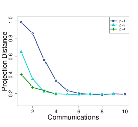
(a) Effect of $p$

(b) Effect of $\varepsilon$

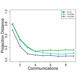
(c) Effect of $\frac{K}{m}$

Figure 3: The numerical performance of FedPower under Model I. We vary $p$, $\varepsilon$, and $\frac{K}{m}$ in (a), (b), and (c) respectively to show their effects on the performance of FedPower.

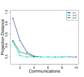
(a) Effect of $p$

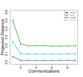
(b) Effect of $\varepsilon$

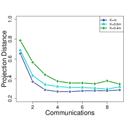
(c) Effect of $\frac{K}{m}$

Figure 4: The numerical performance of FedPower under Model II. We vary $p$, $\varepsilon$, and $\frac{K}{m}$ in (a), (b), and (c) respectively to show their effects on the performance of FedPower.

6 Conclusion and Discussion

We present FedPower, a distributed algorithm designed for the federated learning framework to address the eigenspace estimation problem while ensuring communication efficiency, privacy preservation, and tolerance to stragglers. Our approach involves performing multiple noisy local power iterations between consecutive communications on each worker machine, where the noise comes from the DP’s requirement. Full or partial aggregation scheme is performed after every $p$ iterates. Methodologically, our algorithms provide a flexible and general framework for the computation of leading eigenspace in the modern machine learning setting. Theoretically, our analysis gives a new application of the noisy power method (Hardt and Price, 2014) by combining the perturbed iterate analysis. In addition, the proposed algorithms can be applied to a wide range of statistical and machine learning tasks, including matrix completion, clustering, and ranking, among others.

This work is a first step towards the power-method-based leading eigenspace estimation in the realistic federated learning regime. There are several challenges and open problems that require further investigation. First, the coupled factors $Z_{t}^{(i)}$ and $R_{t}^{(i)}$ in $W_{t}:=\sum_{i}W_{t}^{(i)}$ (see, e.g., (A.5)) make $\|W_{t}\|_{2}$ challenging to bound. In this work, we bound $\|W_{t}\|_{2}$ by taking maximization over all $i\in[m]$ and analyzing each $\|W_{t}^{(i)}\|_{2}$ respectively. However, ideally, one may hope that the summation is left inside the spectral norm and the bound of $\|W_{t}\|_{2}$ depends on the overall error $\|\sum_{i}A_{i}-A\|_{2}$ like the one-shot framework of Charisopoulos et al. (2021). In that case, the theoretical dependence on the heterogeneity parameter $\eta$ can also be relaxed. Therefore, new analyzing tools are in urgent need.

Second, it is well-known that privacy can be amplified by subsampling, that is, a DP mechanism run on a random subsample of a dataset provides higher privacy guarantees than when run on the entire dataset. Most literature considers the sampling without replacement strategy, including Possion subsampling and uniform subsampling. The privacy bound of the sampling without replacement strategy is easy to analyze. Due to technical challenges, very few literature consider the sampling with replacement strategy. In particular, Balle et al. (2018) provides a tight analysis of the privacy bound of the Gaussian mechanism by using the tools of privacy profiles. In our context, the subsampling of local machines ideally can lead to privacy amplification by a factor $K/m$. However, since our algorithm is not additive Gaussian noise perturbation, the privacy profile is difficult to compute. Thus, the tools of sampling with replacement in Balle et al. (2018) are not applicable. Therefore, in terms of privacy analysis, the privacy amplification of the sampling with replacement is harder than that of the sampling without replacement. While in terms of the utility analysis, the non-dependency of local machines in the sampling without replacement strategy would make the analysis challenging. Therefore, whatever the sampling strategy is, the privacy analysis and utility analysis can not be satisfied simultaneously. New concentration inequality on the sum of uniformly sampled (without replacement) matrices and new privacy amplification bound for sampling with replacement strategy without using the privacy profile is imperative.

Third, we mainly consider the curious-but-honest attacker who can see the parameters via communication. In some cases, there also exists an external adversary who only can see the final published results with additional prior information. For example, people who participate in the data collection and model design may be such kind of attackers. Hence, it is beneficial to see how much privacy the FedPower leaks to the external adversary. For the same noise, the privacy leakage (namely, the privacy budget $\varepsilon$) to the external adversary is hopefully smaller than that to the curious onlooker. However, in our context, the DP’s noise to the external adversary is the average of OPT transformed Gaussian random matrices, which makes it difficult to quantify the corresponding privacy leakage. This problem deserves further study.

Appendix

Subsection A and B includes the proofs (also the proof sketch if necessary) corresponding to the full and partial participation protocols, respectively. Subsection C contains the technical lemmas. Subsection D presents auxiliary lemmas used in the proofs. Subsection E introduces the formal definitions and lemmas on metrics between two subspaces.

A. Full participation

Proof of Theorem 6

We provide the proof in the following steps.

First step: Bounding the sensitivity.

Without loss of generality, consider the $i$-th local machine in $t$-th iteration. Let $[Z_{t-1}^{(i)}]_{\cdot l}$ denote the $l$-th ($1\leq l\leq r$) column of $Z_{t-1}^{(i)}$ and let $A_{i}^{\prime}=\frac{m}{n}M_{i}^{\prime\intercal}M_{i}^{\prime}$ be the neighboring dataset of $A_{i}=\frac{m}{n}M_{i}^{\intercal}M_{i}$, where $M_{i}$ and $M_{i}^{\prime}$ differ in one row (denoted by $\omega$ and $\omega^{\prime}$) and all their rows are normalized to have Euclidean norm 1. Conditioning on $[Z_{t-1}^{(i)}]_{\cdot l}$, we have that the $l_{2}$-sensitivity of $A_{i}[Z_{t-1}^{(i)}]_{\cdot l}$ is

$$\|A_{i}[Z_{t-1}^{(i)}]_{\cdot l}-A_{i}^{\prime}[Z_{t-1}^{(i)}]_{\cdot l}\|_{2} \leq\|A_{i}-A_{i}^{\prime}\|_{2}\cdot\|[Z_{t-1}^{(i)}]_{\cdot l}\|_{2}\leq\|A_{i}-A_{i}^{\prime}\|_{\tiny F}$$

$$=\frac{m}{n}\|\omega\omega^{\intercal}-\omega^{\prime}\omega^{\prime\intercal}\|_{\tiny F}\leq\frac{m}{n}(\|\omega\omega^{\intercal}\|_{\tiny F}+\|\omega^{\prime}\omega^{\prime\intercal}\|_{\tiny F})$$

$$=\frac{m}{n}(\|\omega\|_{2}\|\omega\|_{2}+\|\omega^{\prime}\|_{2}\|\omega^{\prime}\|_{2})=\frac{2m}{n}.$$

Stacking $r$ such vectors together to obtain a $d\times r$-dimensional vector, we have that the total sensitivity of $A_{i}Z_{t-1}^{(i)}$ is bounded by $\sqrt{r}\cdot\frac{2m}{n}$.

Second step: Tight composition of RDP.

Suppose that we add i.i.d. Gaussian noise to each entry of $A_{i}Z_{t-1}^{(i)}$ according to

$${Y_{t}^{(i)}=A_{i}Z_{t-1}^{(i)}+\mathcal{N}(0,(\frac{2\sqrt{r}m}{n}\sigma_{g})^{2})^{{d\times r}},}$$

then by Proposition 2, conditioning on $Z_{t-1}^{(i)}$, we have that the above mechanism satisfies $(\alpha,\frac{\alpha}{2\sigma_{g}^{2}})$-RDP.

After $p$ local iterations and $\lfloor T/p\rfloor$ communication rounds, by invoking the adaptive composition theorem of RDP in Proposition 3, we have that Algorithm 2 satisfies $(\alpha,\frac{T\alpha}{2\sigma_{g}^{2}})$-RDP.

Third step: Optimizing $\alpha$ and choosing $\sigma_{g}$.

To be interpretable, we convert RDP to DP via Proposition 5, that is, Algorithm 2 satisfies $(\frac{T\alpha}{2\sigma_{g}^{2}}+\frac{\log(1/\delta)}{\alpha-1},\delta)$-RDP for any $\alpha>1$ and $\delta>0$. To select an optimal $\alpha$, we consider the following optimization problem,

$$\underset{\alpha>1}{\min}\;\varepsilon(\alpha):=\frac{T\alpha}{2\sigma_{g}^{2}}+\frac{\log(1/\delta)}{\alpha-1}.$$ (A.1)

It is easy to obtain that the optimal $\alpha$ for (A.1) is

$$\alpha_{\rm opt}:=1+\sqrt{2\sigma_{g}^{2}\log(1/\delta)/T},$$

and the corresponding $\varepsilon(\alpha_{\rm opt})$ is

$$\varepsilon(\alpha_{\rm opt}):=\frac{T}{2\sigma_{g}^{2}}+\frac{2\sqrt{T\log(1/\delta)}}{\sqrt{2}\cdot\sigma_{g}}.$$ (A.2)

Finally, letting the two parts of RHS of (A.2) both smaller than $\varepsilon/2$, we obtain the following choice of $\sigma_{g}$

$$\sigma_{g}\geq\max\{\sqrt{\frac{T}{\varepsilon}},\;\frac{2\sqrt{2T\log(1/\delta)}}{\varepsilon}\}.$$

As a result, Algorithm 2 attains $(\varepsilon,\delta)$-DP with the variance of Gaussian noise $\nu:=\frac{2\sqrt{r}m}{n}\sigma_{g}\geq\frac{2\sqrt{r}m}{n}\max\{\sqrt{\frac{T}{\varepsilon}},\;\frac{2\sqrt{2T\log(1/\delta)}}{\varepsilon}\}$. $\blacksquare$

Proof of Theorem 7

Proof sketch of Theorem 7: First, we define a virtual sequence

$$\overline{Z}_{t}=\frac{1}{m}\sum_{i=1}^{m}Z_{t}^{(i)}O_{t}^{(i)}.$$

Here $O_{t}^{(i)}\in\mathbb{R}^{r\times r}$ is defined as

$$O_{t}^{(i)}=\begin{cases}\mathbb{I}_{r}&\text{if}\ t\in\mathcal{I}_{T}^{p}\\ D_{t+1}^{(i)}&\text{if}\ t\notin\mathcal{I}_{T}^{p}.\end{cases}$$

Then, we will write $\overline{Z}_{t}$ in the following recursive manner,

$$\overline{Z}_{t}=[A\overline{Z}_{t-1}+\mathcal{G}_{t}]R_{t}^{-1},$$

where $R_{t}$ is a reversible matrix to be defined, and $\mathcal{G}_{t}$ is some noisy perturbation coming from the Gaussian noise incurred by DP and local iterates. To analyze the convergence of FedPower, we use the analytical framework of noisy power iterates in (Hardt and Price, 2014). However, their results require $\overline{Z}_{t}$ to have orthonormal columns, which is not met in our setting. As a remedy, we obtain the following results, which is a modification of Corollary 1.1 (see Lemma 18) in (Hardt and Price, 2014).

Lemma 10 (Informal version of Lemma 12).

Let $\overline{Z}_{0}$ be the orthonormalized space of a $d\times r$ random matrix with each entry being i.i.d. standard Gaussian. Assume $\overline{Z}_{t}$ iterates as follows,

$$\overline{Z}_{t}\leftarrow A\overline{Z}_{t-1}+\mathcal{G}_{t}.$$

If $\mathcal{G}_{t}$ satisfies

$$5\|\mathcal{G}_{t}\|_{2}\leq\epsilon(\sigma_{k}-\sigma_{k+1}){\rm min}_{t}\|\overline{Z}_{t}\|_{\tiny{\rm m}}\quad{\rm and}\quad 5\|U_{k}^{\intercal}\mathcal{G}_{t}\|_{2}\leq(\sigma_{k}-\sigma_{k+1}){\rm min}_{t}\|\overline{Z}_{t}\|_{\tiny{\rm m}}\frac{\sqrt{r}-\sqrt{k-1}}{\tau\sqrt{d}},$$

for some fixed $\tau$ and $\epsilon<1/2$. Then with high probability, there exists an $T=O(\frac{\sigma_{k}}{\sigma_{k}-\sigma_{k+1}}{\rm log}(d\tau/\epsilon))$ so that after $T$ steps

$$\|(\mathbb{I}-\overline{Z}_{T}\overline{Z}_{T}^{\intercal})U_{k}\|_{2}\leq\epsilon.$$

The result also holds for the following iterates with any reversible matrix $R_{t}$,

$$\overline{Z}_{t}\leftarrow[A\overline{Z}_{t-1}+\mathcal{G}_{t}]R_{t}^{-1}.$$

In light of this result, the convergence of Algorithm 2 could be established if we could bound the perturbation error induced from un-synchronization and DP. $\blacksquare$

Proof.

We provide a proof in three steps.

First step: Perturbed iterate analysis.

Recall that we defined a virtual sequence by

$$\overline{Z}_{t}=\frac{1}{m}\sum_{i=1}^{m}Z_{t}^{(i)}O_{t}^{(i)},$$

where $O_{t}^{(i)}$ is $\mathbb{I}_{r}$ if $t\in\mathcal{I}_{T}^{p}$, and is $D_{t+1}^{(i)}$ defined by

$$D_{t+1}^{(i)}=\underset{D\in\mathcal{F}\cap\mathcal{O}_{r}}{{\rm argmin}}\;\|Z_{t}^{(i)}D-Z_{t}^{(1)}\|_{o},$$

if $t\notin\mathcal{I}_{T}^{p}$. Now we discuss the recursive iteration of $\overline{Z}_{t}$ under $t\notin\mathcal{I}_{T}^{p}$ and $t\in\mathcal{I}_{T}^{p}$, respectively. We will use repeatedly the fact that $Y_{t}^{(i)}=Z_{t}^{(i)}R_{t}^{(i)}$ in the following proof.

When $t\notin\mathcal{I}_{T}^{p}$, we note that $Y_{t}^{(i)}=A_{i}Z_{t-1}^{(i)}+N_{t}^{(i)}$, where $N_{t}^{(i)}$ has i.i.d. $\mathcal{N}(0,\nu^{2})$ entries. Then, given any invertible $R_{t}$ (to be specified in Lemma 13), we have

$$\overline{Z}_{t} =\frac{1}{m}\sum_{i=1}^{m}Z^{(i)}_{t}O^{(i)}_{t}$$

$$=\frac{1}{m}\sum_{i=1}^{m}A_{i}Z^{(i)}_{t-1}O^{(i)}_{t-1}R_{t}^{-1}+\frac{1}{m}\sum_{i=1}^{m}Z^{(i)}_{t}[O_{t}^{(i)}R_{t}-R_{t}^{(i)}O_{t-1}^{(i)}]R_{t}^{-1}+\frac{1}{m}\sum_{i=1}^{m}N^{(i)}_{t}O_{t-1}^{(i)}R^{-1}_{t}$$

$$:=(A\overline{Z}_{t-1}+H_{t}+W_{t}+N_{t})R_{t}^{-1},$$ (A.3)

where

$$H_{t}:=\frac{1}{m}\sum_{i=1}^{m}H_{t}^{(i)}:=\frac{1}{m}\sum_{i=1}^{m}(A_{i}-A)Z_{t-1}^{(i)}O_{t-1}^{(i)},$$ (A.4)

$$W_{t}:=\frac{1}{m}\sum_{i=1}^{m}W_{t}^{(i)}:=\frac{1}{m}\sum_{i=1}^{m}Z_{t}^{(i)}[O_{t}^{(i)}R_{t}-R^{(i)}_{t}O_{t-1}^{(i)}],$$ (A.5)

and

$$N_{t}=\frac{1}{m}\sum_{i=1}^{m}N_{t}^{(i)}O_{t-1}^{(i)}.$$

When $t\in\mathcal{I}_{T}^{p}$, synchronization happens. In such case, $R^{(i)}_{t}$’s are identical for all $i\in[m]$ and we let them be $R_{t}$; see Lemma 13 for details, and

$$Y^{(i)}_{t}=\frac{1}{m}\sum_{l=1}^{m}[A_{l}Z^{(l)}_{t-1}D^{(l)}_{t}+N_{t}^{(l)}D_{t}^{(l)}],$$

for all $i\in[m]$. Hence,

$$\overline{Z}_{t} =\frac{1}{m}\sum_{i=1}^{m}Z^{(i)}_{t}O^{(i)}_{t}$$

$$=(\frac{1}{m}\sum_{i=1}^{m}A_{i}Z^{(i)}_{t-1}D^{(i)}_{t}+\frac{1}{m}\sum_{i=1}^{m}Z^{(i)}_{t}[O_{t}^{(i)}R_{t}-R_{t}^{(i)}]+\frac{1}{m}\sum_{i=1}^{m}N_{t}^{(i)}D_{t}^{(i)})R_{t}^{-1}$$

$$=(\frac{1}{m}\sum_{i=1}^{m}A_{i}Z^{(i)}_{t-1}O^{(i)}_{t-1}+\frac{1}{m}\sum_{i=1}^{m}Z^{(i)}_{t}[R_{t}-R_{t}^{(i)}]+\frac{1}{m}\sum_{i=1}^{m}N_{t}^{(i)}D_{t}^{(i)})R_{t}^{-1}$$

$$:=(A\overline{Z}_{t-1}+H_{t}+N^{\prime}_{t})R_{t}^{-1},$$ (A.6)

where we used the fact that $O_{t}^{(i)}=\mathbb{I}_{r}$, $O_{t-1}^{(i)}=D^{(i)}_{t}$, and $R_{t}=R_{t}^{(i)}$; $H_{t}$ is defined in (A.4), and

$$N_{t}^{\prime}:=\frac{1}{m}\sum_{i=1}^{m}N_{t}^{(i)}D_{t}^{(i)}.$$

Second step: Bound the noise term.

We proceed to bound $\|H_{t}\|_{2},\|W_{t}\|_{2}$, $\|N_{t}\|_{2}$ and $\|N^{\prime}_{t}\|_{2}$, respectively.

$\bullet$ For $\|H_{t}\|_{2}$, we have

$$\|H_{t}\|_{2} =\|\frac{1}{m}\sum_{i=1}^{m}H_{t}^{(i)}\|_{2}=\frac{1}{m}\sum_{i=1}^{m}\|\left(A_{i}-A\right)Z_{t-1}^{(i)}O_{t-1}^{(i)}\|_{2}$$

$$\leq\frac{1}{m}\sum_{i=1}^{m}\|A_{i}-A\|_{2}\|Z_{t-1}^{(i)}O_{t-1}^{(i)}\|_{2}\leq\eta\sigma_{1},$$ (A.7)

where the last inequality follows from Definition 4.

$\bullet$ For $\|W_{t}\|_{2}$, we have

$$\|W_{t}\|_{2} =\big{\|}\frac{1}{m}\sum_{i=1}^{m}W_{t}^{(i)}\|_{2}=\frac{1}{m}\sum_{i=1}^{m}\big{\|}Z_{t}^{(i)}\left(O_{t}^{(i)}R_{t}-R_{t}^{(i)}O_{t-1}^{(i)}\right)\big{\|}_{2}$$

$$\leq\frac{1}{m}\sum_{i=1}^{m}\big{\|}O_{t}^{(i)}R_{t}-R_{t}^{(i)}O_{t-1}^{(i)}\big{\|}_{2}.$$

Here, a good choice of $R_{t}$ should be specified to ensure a tight bound of $\|W_{t}\|_{2}$. Specifically, $R_{t}$ is chosen in a recursive manner as we show in Lemma 13 in the Appendix C. In particular, we prove in Lemma 13 that for any $i\in[m]$

$$\|O_{t}^{(i)}R_{t}-R_{t}^{(i)}O_{t-1}^{(i)}\|_{2} \leq\sigma_{1}(A_{1})\|Z_{t}^{(i)}O_{t}^{(i)}-Z_{t}^{(1)}\|_{2}+\|A_{1}-A_{i}\|_{2}+\sigma_{1}(A_{i})\|Z_{t-1}^{(i)}O_{t-1}^{(i)}-Z_{t-1}^{(1)}\|_{2}$$

$$\leq{2}\sigma_{1}\left(\rho_{t}+\eta+(1+\eta)\rho_{t-1}\right),$$ (A.8)

where we make use of Definition 4 and define

$$\rho_{t}={\rm max}_{i}\|Z_{t}^{(i)}O_{t}^{(i)}-Z_{t}^{(1)}\|_{2}={\rm max}_{i}\|Z_{t}^{(i)}D_{t+1}^{(i)}-Z_{t}^{(1)}\|_{2},$$ (A.9)

with $\rho_{t}$ upper bounded as in (3.6) and (3.7); see Lemma 14 and 15 for details. As a result, we obtain

$$\|W_{t}\|_{2}\leq 2\sigma_{1}\left(\rho_{t}+\eta+(1+\eta)\rho_{t-1}\right).$$ (A.10)

$\bullet$ For $\|N_{t}\|_{2}$, we recall that

$$N_{t}=\frac{1}{m}\sum_{i=1}^{m}N_{t}^{(i)}O_{t-1}^{(i)},$$

where $N_{t}^{(i)}$ is a random matrix with each entry being i.i.d. $\mathcal{N}(0,\nu^{2})$. We will make use of Bernstein-type concentration inequality developed for sums of a random matrix multiplied by a non-random matrix ((Lei and Lin, 2022), see also Lemma 20) to proceed. We first observe that $Y\sim\mathcal{N}(0,\nu^{2})$ is $(2\nu^{2},\nu^{2})$-Bernstein (see Definition 6) because for non-negative integer $q$,

$$\mathbb{E}|Y|^{q}\leq\nu^{q}(q-1)!\leq\frac{2\nu^{2}}{2}q!\nu^{q-2},$$ (A.11)

where the first inequality follows from Lemma 21. Then by conditioning on $O_{t-1}^{(i)}$’s and Lemma 20, we have

$$\mathbb{P}(\|N_{t}\|_{2}\geq t)=\mathbb{P}(\|\sum_{i=1}^{m}N_{t}^{(i)}O_{t-1}^{(i)}\|_{2}\geq mt)\leq 4d\exp\left(-\frac{m^{2}t^{2}/2}{2\nu^{2}dm+\nu tm}\right)$$ (A.12)

Let

$$t_{\rm opt}\asymp\sqrt{4d\nu^{2}\log(dT)/m}+\nu\log(dT)/m,$$

we then have with probability larger than $1-(dT)^{-\gamma}$ for some $\gamma>1$ that

$$\|N_{t}\|_{2}\leq t_{\rm opt}\lesssim{\nu}\max\left\{\sqrt{\frac{d\log(dT)}{m}},\;\frac{\log(dT)}{m}\right\}.$$ (A.13)

Further, by the union bound, $\max_{t}\|N_{t}\|_{2}$ is also bounded by the RHS of (A.13) but with probability $1-(dT)^{-\alpha}$ for some $\alpha>0$.

$\bullet$ For $\|N_{t}^{\prime}\|_{2}$, we can use the same technique as that for bounding $\|N_{t}\|_{2}$ and the same bound can be derived.

Combining (Second step: Bound the noise term.), (A.10) and (A.13) and recalling the expression (First step: Perturbed iterate analysis.) and (First step: Perturbed iterate analysis.), we obtain that the perturbation noise $\mathcal{G}_{t}:=H_{t}+W_{t}+N_{t}+N^{\prime}_{t}$ satisfies that

$${\rm max}_{t}\|\mathcal{G}_{t}\|_{2}\lesssim{\nu}\max\left\{\sqrt{{d\log(dT)}/{m}},\;{\log(dT)}/{m}\right\}+2\sigma_{1}\left(\eta+(2+\eta){\rm max}_{t}\rho_{t}\right),$$ (A.14)

with probability larger than $1-(dT)^{-\alpha}$ for some $\alpha>0$. To lighten the notation, we denote the RHS of (A.14) by ${\rm Err}(\nu,\sigma_{1},d,m,T,p,k,\eta)$.

Third step: Establish convergence.

Now we make use of the result in Lemma 12 to establish convergence. Note that in Lemma 12, there still exists an unknown term $\|\overline{Z}_{t}\|_{\rm\tiny m}$. We prove in Lemma 16 that

$$\|\overline{Z}_{t}\|_{\rm\tiny m}\geq 1-(1-1/m){\rm max}_{t}\rho_{t}.$$

Denote

$$\epsilon^{\prime}:=\frac{{\rm Err}(\nu,\sigma_{1},d,m,T,p,k,\eta)}{(\sigma_{k}-\sigma_{k+1})(1-(1-1/m){\rm max}_{t}\rho_{t})},$$

then by (A.14),

$$5{\rm max}_{t}\|\mathcal{G}_{t}\|_{2}\leq\epsilon^{\prime}(\sigma_{k}-\sigma_{k+1})\|\overline{Z}_{t}\|_{\rm\tiny m}.$$ (A.15)

Hence the first condition in Lemma 12 is satisfied. For the second condition, we have that

$$5{\rm max}_{t}\|U_{k}^{\intercal}\mathcal{G}_{t}\|_{2}\leq 5{\rm max}_{t}\|\mathcal{G}_{t}\|_{2},$$

which implies that the second condition would be met automatically if $\epsilon^{\prime}<\frac{\sqrt{r}-\sqrt{k-1}}{\tau\sqrt{d}}$, which is our condition. Consequently, by Lemma 12, we have after $T=O(\frac{\sigma_{k}}{\sigma_{k}-\sigma_{k+1}}{\rm log}(\frac{d}{\epsilon^{\prime}}))$ iterations,

$$\|(\mathbb{I}_{d}-\overline{Z}_{T}\overline{Z}_{T}^{\intercal})U_{k}\|_{2}\leq\epsilon^{\prime},$$

with probability larger than $1-(dT)^{-\alpha}-\tau^{-\Omega(r+1-k)}-e^{-\Omega(d)}$. ∎

Proof of Theorem 8

By Lemma 14 and 15, the following results hold.

• If $\mathcal{F}=\mathcal{O}_{r}$, then

  $$\rho_{t}\leq\sqrt{2}\min\left\{\frac{2\kappa^{p}\eta(1+\eta)^{p-1}}{(1-\eta)^{p}},\frac{\eta\sigma_{1}}{\delta_{k}}+2\gamma_{k}^{p/4}\max_{i\in[m]}\tan\theta_{k}(Z_{\tau(t)},U_{k}^{(i)})\right\}.$$

  with the parameters $\delta_{k}={\rm min}_{i\in[m]}\delta_{k}^{(i)}$ with $\delta_{k}^{(i)}={\rm min}\{|\sigma_{j}(A_{i})-\sigma_{k}(A)|:j\geq k+1\}$ and $\gamma_{k}={\rm max}\{{\rm max}_{i\in[m]}\frac{\sigma_{k+1}(A_{i})}{\sigma_{k}(A_{i})},\frac{\sigma_{k+1}(A)}{\sigma_{k}(A)}\}$. By requiring $\eta\kappa\leq 1/3$, and Wely’s inequality, we have

  $$\sigma_{{j}}(A)-\sigma_{k}(A)-\frac{1}{3}\sigma_{d}(A)\leq\sigma_{j}(A_{i})-\sigma_{k}(A)\leq\sigma_{{j}}(A)-\sigma_{k}(A)+\frac{1}{3}\sigma_{d}(A).$$

  Hence, $\delta_{k}\asymp\sigma_{k}(A)-\sigma_{k+1}(A)$. By requiring $\eta\leq 1/p$, we have $\frac{(1+\eta)^{p-1}}{(1-\eta)^{p}}\leq\frac{(1+1/p)^{p-1}}{(1-1/p)^{p}}\leq\mathrm{e}^{2}$. Define $C_{t}=\max_{i\in[m]}{\rm tan}\theta_{k}(Z_{\tau(t)},U_{k}^{(i)})$. Actually, we have shown in Theorem 7 that $\sin\theta_{k}(Z_{\tau(t)},U_{k})\leq\epsilon^{\prime}$ for sufficiently large $t$. By the condition that $\epsilon^{\prime}$ is small enough, we can obtain $\lim\limits_{t\to\infty}\theta_{k}(Z_{\tau(t)},U_{k})=0$. Then, we have

  $$\limsup\limits_{t\to\infty}C_{t}=\limsup\limits_{t\to\infty}\max_{i\in[m]}{\rm tan}\,\theta_{k}(Z_{\tau(t)},U_{k}^{(i)})\leq\max_{i\in[m]}{\tan}\,\theta_{k}(U_{k},U_{k}^{(i)})\leq\max_{i\in[m]}{\tan}\arg\sin\frac{\eta\sigma_{1}}{\delta_{k}}=O(\eta),$$

  where the last inequality follows from the Davis-Kahan theorem (see Lemma 23).

• If $\mathcal{F}=\{\mathbb{I}_{r}\}$, then

  $$\rho_{t}\leq 4\sqrt{2k}p\kappa^{p}\eta(1+\eta)^{p-1}\leq 4\mathrm{e}\sqrt{2k}p\kappa^{p}\eta,$$

  where the last inequality requires $\eta\leq 1/p$.

Simply put together, we confirm that the bounds of $\rho_{t}$ in Theorem 8 hold. $\blacksquare$

B. Partial participation

Proof of Theorem 9

Proof sketch of Theorem 9: Similar to the proof under the full participation setting, we consider the virtual sequence

$$\overline{Z}_{t}:=\frac{1}{K}\sum_{i\in\mathcal{S}_{\tau(t)}}Z_{t}^{(i)}O_{t}^{(i)},$$ (B.1)

where $O_{t}^{(i)}$ is $\mathbb{I}_{r}$ if $t\in\mathcal{I}_{T}^{p}$, and is $D_{t+1}^{(i)}$ defined by

$$D_{t+1}^{(i)}=\underset{D\in\mathcal{F}\cap\mathcal{O}_{r}}{{\rm argmin}}\;\|Z_{t}^{(i)}D-Z_{t}^{(1)}\|_{o},$$

if $t\notin\mathcal{I}_{T}^{p}$. We will write $\overline{Z}_{t}$ in the following recursive manner,

$$\overline{Z}_{t}=[A\overline{Z}_{t-1}+\mathcal{G}_{t}]R_{t}^{-1},$$

where $R_{t}^{-1}$ is the a reversible matrix to be specified, and $\mathcal{G}_{t}$ is some noisy perturbations which turns out to come from three sources. Except for the DP’s noise and the local iterates’ perturbation, the random sampling of local machines also contributes to $\mathcal{G}_{t}$. To be specific, when $\tau(t)\neq\tau(t-1)$, it holds with high probability that $\mathcal{S}_{\tau(t)}\neq\mathcal{S}_{\tau(t-1)}$. Thus we also need to bound the bias term that the random sampling of local machines brings. With $\mathcal{G}_{t}$ properly bounded, the convergence of would be established using Lemma 12. $\blacksquare$

Proof.

We provide a proof in three steps.

First step: Perturbed iterate analysis.

Now we proceed to derive the recursive iteration of $\overline{Z}_{t}$ under $t\notin\mathcal{I}_{T}^{p}$ and $t\in\mathcal{I}_{T}^{p}$, respectively. We will use repeatedly the fact that $Y_{t}^{(i)}=Z_{t}^{(i)}R_{t}^{(i)}$ in the following proof.

When $t\notin\mathcal{I}_{T}^{p}$, we have $Y_{t}^{(i)}=A_{i}Z_{t-1}^{(i)}+N_{t}^{(i)}$, where $N_{t}^{(i)}$ has i.i.d. $\mathcal{N}(0,\nu^{2})$ entries. Thus, given any invertible $R^{t}$ (to be specified in Lemma 13), we have

$$\overline{Z}_{t} =\frac{1}{K}\sum_{i\in\mathcal{S}_{\tau(t)}}Z_{t}^{(i)}O_{t}^{(i)}$$

$$=\frac{1}{K}\sum_{i\in\mathcal{S}_{\tau(t)}}AZ^{(i)}_{t-1}O_{t-1}^{(i)}R_{t}^{-1}+\frac{1}{K}\sum_{i\in\mathcal{S}_{\tau(t)}}(A_{i}-A)Z^{(i)}_{t-1}O_{t-1}^{(i)}R_{t}^{-1}$$

$$\quad\quad\quad\quad\quad+\frac{1}{K}\sum_{i\in\mathcal{S}_{\tau(t)}}Z^{(i)}_{t}[O_{t}^{(i)}R_{t}-R_{t}^{(i)}O_{t-1}^{(i)}]R^{-1}_{t}+\frac{1}{K}\sum_{i\in\mathcal{S}_{\tau(t)}}N_{t}^{(i)}O_{t-1}^{(i)}R^{-1}_{t}$$

$$:=(\mathcal{J}_{t}+H_{t}+W_{t}+N_{t})R_{t}^{-1},$$ (B.2)

for which $\mathcal{J}_{t}$ could be further expressed as

$$\mathcal{J}_{t} =\frac{1}{K}\sum_{i\in\mathcal{S}_{\tau(t-1)}}AZ^{(i)}_{t-1}O_{t-1}^{(i)}+\frac{1}{K}\left(\sum_{i\in\mathcal{S}_{\tau(t)}}AZ^{(i)}_{t-1}O_{t-1}^{(i)}-\sum_{i\in\mathcal{S}_{\tau(t-1)}}AZ^{(i)}_{t-1}O_{t-1}^{(i)}\right)$$

$$=A\overline{Z}_{t-1}+\left(\sum_{i\in\mathcal{S}_{\tau(t)}}AZ^{(i)}_{t-1}O_{t-1}^{(i)}/K-\mathbb{E}_{\mathcal{S}_{\tau(t)}}[\sum_{i\in\mathcal{S}_{\tau(t)}}AZ^{(i)}_{t-1}O_{t-1}^{(i)}/K]\right)$$

$$\quad\quad\quad\quad\quad\quad\quad\quad\quad\quad\quad\quad\quad\quad\quad\quad\quad\quad\quad+\left(\mathbb{E}_{\mathcal{S}_{\tau(t)}}[\sum_{i\in\mathcal{S}_{\tau(t)}}AZ^{(i)}_{t-1}O_{t-1}^{(i)}/K]-\sum_{i\in\mathcal{S}_{\tau(t-1)}}AZ^{(i)}_{t-1}O_{t-1}^{(i)}/K\right)$$

$$=A\overline{Z}_{t-1}+\left(\sum_{i\in\mathcal{S}_{\tau(t)}}AZ^{(i)}_{t-1}O_{t-1}^{(i)}/K-\sum_{i=1}^{m}AZ_{t-1}^{(i)}O_{t-1}^{(i)}/m\right)+\left(\sum_{i=1}^{m}AZ_{t-1}^{(i)}O_{t-1}^{(i)}/m-\sum_{i\in\mathcal{S}_{\tau(t-1)}}AZ^{(i)}_{t-1}O_{t-1}^{(i)}/K\right)$$

$$:=A\overline{Z}_{t-1}+E_{t}+F_{t},$$ (B.3)

where the expectation only involves the randomness from sampling the local machines. Combining (First step: Perturbed iterate analysis.) with (First step: Perturbed iterate analysis.), we obtain when $t\notin\mathcal{I}^{p}_{T}$ that,

$$\overline{Z}_{t}=(A\overline{Z}_{t-1}+E_{t}+F_{t}+H_{t}+W_{t}+N_{t})R_{t}^{-1}.$$ (B.4)

When $t\in\mathcal{I}^{p}_{T}$, the synchronization happens. Thereby, for all $i\in\mathcal{S}_{\tau(t)}$,

$$Y_{t}^{(i)} =\frac{1}{K}\sum_{l\in\mathcal{S}_{\tau(t)}}(A_{l}Z_{t-1}^{(l)}D_{t}^{(l)}+N_{t}^{(l)}D_{t}^{(l)}):=\frac{1}{K}\sum_{l\in\mathcal{S}_{\tau(t)}}A_{l}Z_{t-1}^{(l)}D_{t}^{(l)}+N^{\prime}_{t}.$$ (B.5)

Using similar treatments as in (First step: Perturbed iterate analysis.) and (First step: Perturbed iterate analysis.), we have when $t\in\mathcal{I}^{p}_{T}$ that,

$$\overline{Z}_{t}=(A\overline{Z}_{t-1}+E_{t}+F_{t}+H_{t}+N^{\prime}_{t})R_{t}^{-1},$$ (B.6)

where note that similar to the full participation protocol, $W_{t}$ does not appear when $t\in\mathcal{I}^{p}_{T}$.

Second step: Bound the noise term.

We proceed to bound $E_{t}$, $F_{t}$, $H_{t}$, $W_{t}$, $N_{t}$ and $N^{\prime}_{t}$, respectively.

$\bullet$ For $\|E_{t}\|_{2}$, we denote

$$E_{t} :=A\sum_{i\in\mathcal{S}_{\tau(t)}}\frac{1}{K}\left(Z^{(i)}_{t-1}O^{(i)}_{t-1}-\frac{1}{m}\sum_{i=1}^{m}Z_{t-1}^{(i)}O^{(i)}_{t-1}\right):=A\sum_{i\in\mathcal{S}_{\tau(t)}}S_{t}^{(i)}:=AS_{t}.$$ (B.7)

We will make use of the matrix Bernstein inequality ((Tropp, 2015), restated in Lemma 22), to bound $\|S_{t}\|_{2}$. Consider only the randomness that the $S_{\tau(t)}$ brings, we have

$$\mathbb{E}_{S_{\tau(t)}}(S_{t}^{(i)})=0\quad{\rm and}\quad\|S_{t}^{(i)}\|_{2}\leq\frac{2}{K},$$

and let

$$\nu(S_{t})={\rm max}\{\|\mathbb{E}(S_{t}S_{t}^{\intercal})\|_{2},\|\mathbb{E}(S_{t}^{\intercal}S_{t})\|_{2}\}.$$ (B.8)

By Lemma 22, we thus have

$$\mathbb{P}(\|S_{t}\|_{2}\geq t)\leq(d+r)\cdot\exp\left(\frac{-t^{2}/2}{\nu(S_{t})+{2t}/{(3K)}}\right).$$ (B.9)

Choosing $t=\sqrt{2\nu(S_{t})\log(T(d+r))}+{2\log(T(d+r))}/{(3K)}$, then (B.9) implies

$$\|S_{t}\|_{2}\lesssim\sqrt{2\nu(S_{t})\log(T(d+r))}+{2\log(T(d+r))}/{(3K)},$$ (B.10)

with probability larger than $1-(T(d+r))^{-\mu}$ for some $\mu>1$. It remains to bound $\nu(S_{t})$. Denote $\xi=\frac{1}{m}\sum_{i=1}^{m}Z_{t-1}^{(i)}O^{(i)}_{t-1}$, then

$$S_{t}S_{t}^{\intercal}=\frac{1}{K^{2}}\sum_{i\in\mathcal{S}_{\tau(t)}}Z^{(i)}_{t-1}O^{(i)}_{t-1}\sum_{i\in\mathcal{S}_{\tau(t)}}(Z^{(i)}_{t-1}O^{(i)}_{t-1})^{\intercal}-\xi\frac{1}{K}\sum_{i\in\mathcal{S}_{\tau(t)}}(Z^{(i)}_{t-1}O^{(i)}_{t-1})^{\intercal}-\frac{1}{K}\sum_{i\in\mathcal{S}_{\tau(t)}}Z^{(i)}_{t-1}O^{(i)}_{t-1}\xi^{\intercal}+\xi\xi^{\intercal}.$$ (B.11)

To shorten the notation, we denote $Z^{o(i)}_{t-1}:=Z^{(i)}_{t-1}O^{(i)}_{t-1}$. Taking expectation with respect to $\mathcal{S}_{\tau(t)}$, we then have

$$\mathbb{E}_{\mathcal{S}_{\tau(t)}}S_{t}S_{t}^{\intercal} =\mathbb{E}_{\mathcal{S}_{\tau(t)}}[\frac{1}{K^{2}}\sum_{i\in\mathcal{S}_{\tau(t)}}Z^{o(i)}_{t-1}\sum_{i\in\mathcal{S}_{\tau(t)}}(Z^{o(i)}_{t-1})^{\intercal}]-\xi\xi^{\intercal}$$

$$=\frac{1}{K^{2}}\mathbb{E}_{\mathcal{S}_{\tau(t)}}[\sum_{i\neq j,i,j\in\mathcal{S}_{\tau(t)}}Z^{o(i)}_{t-1}(Z^{o(j)}_{t-1})^{\intercal}+\sum_{i=j,i,j\in\mathcal{S}_{\tau(t)}}Z^{o(i)}_{t-1}(Z^{o(j)}_{t-1})^{\intercal}]-\xi\xi^{\intercal}$$

$$=\frac{K(K-1)}{K^{2}}\sum_{i\neq j,i,j=1}^{m}\frac{1}{m^{2}}Z^{o(i)}_{t-1}(Z^{o(j)}_{t-1})^{\intercal}+\frac{K}{K^{2}}\sum_{i=j=1}^{m}\frac{1}{m}Z^{o(i)}_{t-1}(Z^{o(j)}_{t-1})^{\intercal}-\sum_{i,j=1}^{m}\frac{1}{m^{2}}Z^{o(i)}_{t-1}(Z^{o(j)}_{t-1})^{\intercal}$$

$$=-\frac{1}{K}\sum_{i\neq j,i,j=1}^{m}\frac{1}{m^{2}}Z^{o(i)}_{t-1}(Z^{o(j)}_{t-1})^{\intercal}+\sum_{i=1}^{m}\frac{1}{m}(\frac{1}{K}-\frac{1}{m})Z^{o(i)}_{t-1}(Z^{o(i)}_{t-1})^{\intercal}.$$ (B.12)

As a result,

$$\|\mathbb{E}_{\mathcal{S}_{\tau(t)}}(S_{t}S_{t}^{\intercal})\|_{2}\leq\frac{1}{K}\sum_{i\neq j,i,j=1}^{m}\frac{1}{m^{2}}+\sum_{i=1}^{m}\frac{1}{m^{2}}+\frac{1}{K}\lesssim\frac{1}{K}.$$ (B.13)

Similarly, we could obtain

$$\|\mathbb{E}_{\mathcal{S}_{\tau(t)}}(S_{t}^{\intercal}S_{t})\|_{2}\lesssim\frac{1}{K}.$$

Consequently, by (B.10), (B.7), and the union bound, we have

$$\underset{t\in\mathcal{I}_{T}^{p}}{\rm max}\|E_{t}+F_{t}\|_{2}\leq\underset{t}{\rm max}2\|E_{t}\|_{2}\lesssim\sigma_{1}\max\left\{\sqrt{\frac{\log(dT)}{K}},\;\frac{\log(dT)}{K}\right\}.$$ (B.14)

with probability larger than $1-(T(d+r))^{-\iota}$ for some $\iota>0$.

$\bullet$ For $\|H_{t}\|_{2}$, similar to the deviation of (Second step: Bound the noise term.), we have

$$\|H_{t}\|_{2}=\|\frac{1}{K}\sum_{i\in\mathcal{S}_{\tau(t)}}(A_{i}-A)Z^{(i)}_{t-1}O^{(i)}_{t-1}\|_{2}\leq\eta\sigma_{1}.$$ (B.15)

$\bullet$ For $\|W_{t}\|_{2}$, similar to the deviation of (A.10), we have

$$\|W_{t}\|_{2}=\|\frac{1}{K}\sum_{i\in\mathcal{S}_{\tau(t)}}Z^{(i)}_{t-1}(O_{t}^{(i)}R_{t}-R_{t}^{(i)}O_{t-1}^{(i)})\|_{2}\leq 2\sigma_{1}\left(\eta+(2+\eta){\rm max}_{t}\rho_{t}\right),$$ (B.16)

where $\rho_{t}$ is defined as

$$\rho_{t}={\rm max}_{i}\|Z_{t}^{(i)}O_{t}^{(i)}-Z_{t}^{(1)}\|_{2}={\rm max}_{i}\|Z_{t}^{(i)}D_{t+1}^{(i)}-Z_{t}^{(1)}\|_{2},$$

and upper bounded as in (3.6) and (3.7); see Lemma 14 and 15 for details.

$\bullet$ For $\|N_{t}\|_{2}$, conditioning on $\mathcal{S}_{\tau(t)}$, using similar tools as for (A.13), we have

$${\rm max}_{t}\|N_{t}\|_{2}\lesssim{\nu}\max\left\{\sqrt{\frac{d\log(dT)}{K}},\;\frac{\log(dT)}{K}\right\}.$$ (B.17)

with probability larger than $1-(dT)^{-\gamma}$ for some $\gamma>0$.

Putting (B.14)-(B.17) together, and recalling (B.4) and (B.6), then the perturbation noise $\mathcal{G}_{t}:=E_{t}+F_{t}+H_{t}+W_{t}+N_{t}+N^{\prime}_{t}$ satisfies that

$${\rm max}_{t} \|\mathcal{G}_{t}\|_{2}\lesssim{\nu}\max\left\{\sqrt{\frac{d\log(dT)}{K}},\;\frac{\log(dT)}{K}\right\}+2\sigma_{1}\left(\eta+(2+\eta){\rm max}_{t}\rho_{t}\right)$$

$$\quad\quad\quad\quad\quad\quad\quad\quad\quad+\sigma_{1}\max\left\{\sqrt{\frac{\log(dT)}{K}},\;\frac{\log(dT)}{K}\right\},$$ (B.19)

with probability larger than $1-(dT)^{-\beta}$ for positive constant $\beta$. For notational simplicity, we denote the RHS of (Second step: Bound the noise term.) as ${\rm Err}(\nu,\sigma_{1},d,m,K,T,p,k,\eta)$

Third step: Establish convergence.

At last, we use Lemma 12 to establish convergence. Denote

$$\epsilon^{\prime\prime}:=\frac{{\rm Err}(\nu,\sigma_{1},d,m,K,T,p,k,\eta)}{(\sigma_{k}-\sigma_{k+1})(1-{\rm max}_{t}\rho_{t})},$$

then by (Second step: Bound the noise term.),

$$5{\rm max}_{t}\|\mathcal{G}_{t}\|_{2}\leq\epsilon^{\prime\prime}(\sigma_{k}-\sigma_{k+1})\|\overline{Z}_{t}\|_{\rm\tiny m},$$

where we used the fact in Lemma 16 that

$$\|\overline{Z}_{t}\|_{\rm\tiny m}\geq 1-{\rm max}_{t}\rho_{t}.$$

The first condition in Lemma 12 is thus satisfied. For the second condition, we have that

$$5{\rm max}_{t}\|U_{k}^{\intercal}\mathcal{G}_{t}\|_{2}\leq 5{\rm max}_{t}\|\mathcal{G}_{t}\|_{2},$$

which implies that the second condition would be met automatically if $\epsilon^{\prime\prime}<\frac{\sqrt{r}-\sqrt{k-1}}{\tau\sqrt{d}}$, which is our condition. Overall, by Lemma 12, we have after $T=O(\frac{\sigma_{k}}{\sigma_{k}-\sigma_{k+1}}{\rm log}(\frac{d}{\epsilon^{\prime\prime}}))$ iterations,

$$\|(\mathbb{I}_{d}-\overline{Z}_{T}\overline{Z}_{T}^{\intercal})U_{k}\|_{2}\leq\epsilon^{\prime\prime},$$

with probability larger than $1-(dT)^{-\beta}-\tau^{-\Omega(r+1-k)}-e^{-\Omega(d)}$ for some positive constants $\beta$ and $\tau$. ∎

C. Technical lemmas

The following lemma is a variant of Lemma 2.2 in (Hardt and Price, 2014) (see Lemma 17). Given the relation $\overline{Z}_{t}=A\overline{Z}_{t-1}+\mathcal{G}_{t}$, they require $\overline{Z}_{t}$ to have orthonormal columns, i.e., $\overline{Z}_{t}^{\intercal}\overline{Z}_{t}=\mathbb{I}_{r}$. However, it is impossible in our analysis. As a remedy, we slightly change the lemma to allow arbitrary $\overline{Z}_{t}$. This will also change the condition on $\mathcal{G}_{t}$.

Lemma 11.

Let $U_{k}\in\mathbb{R}^{d\times k}$ denote the top $k$ eigenvectors of $A$ and let $\sigma_{1}\geq...\geq\sigma_{d}$ denote its eigenvalues. Let $\overline{Z}_{t}\in\mathbb{R}^{d\times r}$ for some $r\geq k$. Let $\mathcal{G}_{t}$ satisfy

$$4\|U_{k}^{\intercal}\mathcal{G}_{t}\|_{2}\leq(\sigma_{k}-\sigma_{k+1}){\rm cos}\,\theta_{k}(U_{k},\overline{Z}_{t})\|\overline{Z}_{t}\|_{\tiny{\rm m}}\quad{\rm and}\quad 4\|\mathcal{G}_{t}\|_{2}\leq(\sigma_{k}-\sigma_{k+1})\|\overline{Z}_{t}\|_{\tiny{\rm m}}\epsilon,$$

for some $\epsilon\leq 1$, where $\|\overline{Z}_{t}\|_{\tiny{\rm m}}$ denotes the minimum singular value of $\overline{Z}_{t}$. Then

$${\rm tan}\,\theta_{k}(U_{k},A\overline{Z}_{t}+\mathcal{G}_{t})\leq{\rm max}\left(\epsilon,{\rm max}\left(\epsilon,\left(\frac{\sigma_{k+1}}{\sigma_{k}}\right)^{1/4}\right){\rm tan}\,\theta_{k}(U_{k},\overline{Z}_{t})\right),$$

where the LHS can be replaced by ${\rm tan}\,\theta_{k}(U_{k},(A\overline{Z}_{t}+\mathcal{G}_{t})R^{-1}_{t})$ with any reversible matrix $R_{t}$.

Proof.

The proof actually follows closely from that of (Hardt and Price, 2014). Hence, we here only show the main steps.

First, by the definition of angles between subspaces, the Lemma 2.2 in (Hardt and Price, 2014) obtain that,

$${\rm tan}\,\theta_{k}(U_{k},A\overline{Z}_{t}+\mathcal{G}_{t})\leq\underset{\|w\|_{2}=1,\Pi^{*}w=w}{{\rm max}}\frac{1}{\|U_{k}^{\intercal}\overline{Z}_{t}w\|_{2}}\cdot\frac{\sigma_{k+1}\|(U_{k}^{\perp})^{\intercal}\overline{Z}_{t}w\|_{2}+\|(U_{k}^{\perp})^{\intercal}\mathcal{G}_{t}w\|_{2}}{\sigma_{k}-\|U_{k}^{\intercal}\mathcal{G}_{t}w\|_{2}/\|U_{k}^{\intercal}\overline{Z}_{t}w\|_{2}},$$

where $\Pi^{*}$ is the matrix projecting onto the smallest $k$ principal angles of $\overline{Z}_{t}$. Define $\Delta=(\sigma_{k}-\sigma_{k+1})/4$. Then, by the assumption on $\mathcal{G}_{t}$,

$$\underset{\|w\|_{2}=1,\Pi^{*}w=w}{{\rm max}}\frac{\|U_{k}^{\intercal}\mathcal{G}_{t}w\|_{2}}{\|U_{k}^{\intercal}\overline{Z}_{t}w\|_{2}}\leq\frac{\|U_{k}^{\intercal}\mathcal{G}_{t}\|_{2}}{{\rm cos}\,\theta_{k}(U_{k},\overline{Z}_{t})\|\overline{Z}_{t}\|_{\tiny{\rm m}}}\leq\Delta,$$

where we used Fact 2 on the principle angle in Appendix E. Similarly, using the fact that ${1/{\rm cos}\,\theta}\leq 1+{\rm tan}\,\theta$ for any angle $\theta$, we have

$$\underset{\|w\|_{2}=1,\Pi^{*}w=w}{{\rm max}}\frac{\|(U_{k}^{\perp})^{\intercal}\mathcal{G}_{t}w\|_{2}}{\|U_{k}^{\intercal}\overline{Z}_{t}w\|_{2}}\leq\frac{\|\mathcal{G}_{t}\|_{2}}{{\rm cos}\,\theta_{k}(U_{k},\overline{Z}_{t})\|\overline{Z}_{t}\|_{\tiny{\rm m}}}\leq\epsilon\Delta(1+{\rm tan}\,\theta_{k}(U_{k},\overline{Z}_{t})).$$

Given the above two inequalities, the remaining proofing strategy is the same as that of (Hardt and Price, 2014). Hence we here omit it. In addition, noting the Fact 1 in Appendix E, we know that the result can be generalized to ${\rm tan}\,\theta_{k}(U_{k},(A\overline{Z}_{t}+\mathcal{G}_{t})R^{-1}_{t})$ with any reversible matrix $R_{t}$. ∎

With Lemma 11, it is easy to derive an analog of Corollary 1.1 in (Hardt and Price, 2014) (see Lemma 18). We summarize the results as the following lemma.

Lemma 12.

Let $k$ and $r$ ($k\leq r$) be the target rank and iteration rank, respectively. Let $U_{k}\in\mathbb{R}^{d\times k}$ denote the top $k$ eigenvectors of $A$ and let ${\sigma_{1}\geq...\geq\sigma_{d}}$ denote its eigenvalues. Suppose $\overline{Z}_{0}$ is the orthonormalized space of $\sim\mathcal{N}(0,\mathbb{I}_{d\times r})$. Assume the noisy power method iterates as follows,

$$\overline{Z}_{t}\leftarrow A\overline{Z}_{t-1}+\mathcal{G}_{t},$$

where $\overline{Z}_{t}$ does not necessarily have orthonormal columns and $\mathcal{G}_{t}$ is some noisy perturbation that satisfies

$$5\|\mathcal{G}_{t}\|_{2}\leq\epsilon(\sigma_{k}-\sigma_{k+1}){\rm min}_{t}\|\overline{Z}_{t}\|_{\tiny{\rm m}}\quad{\rm and}\quad 5\|U_{k}^{\intercal}\mathcal{G}_{t}\|_{2}\leq(\sigma_{k}-\sigma_{k+1}){\rm min}_{t}\|\overline{Z}_{t}\|_{\tiny{\rm m}}\frac{\sqrt{r}-\sqrt{k-1}}{\tau\sqrt{d}},$$

for some fixed $\tau$ and $\epsilon<1/2$. Then with all but $\tau^{-\Omega(r+1-k)}+e^{-\Omega(d)}$ probability, there exists an $T=O(\frac{\sigma_{k}}{\sigma_{k}-\sigma_{k+1}}{\rm log}(d\tau/\epsilon))$ so that after $T$ steps

$$\|(I-\overline{Z}_{T}\overline{Z}_{T}^{\intercal})U_{k}\|_{2}\leq\epsilon.$$

The result also holds for the sequence

$$\overline{Z}_{t}\leftarrow[A\overline{Z}_{t-1}+\mathcal{G}_{t}]R^{-1}_{t},$$

with any reversible $R_{t}$.

Proof.

By Lemma 11 and the proofing techniques of Corollary 1.1 in (Hardt and Price, 2014) (see Lemma 18), the result follows. ∎

In the next lemma, we specify the choice of $R_{t}$ and analyze the residual error bound $\|O_{t}^{(i)}R_{t}-R_{t}^{(i)}O_{t-1}^{(i)}\|_{2}$ when $t\notin\mathcal{I}_{T}^{p}$. In particular, given a baseline data matrix $A_{o}$, $R_{t}$ is the shadow matrix that depicts what the upper triangle matrix ought to be, if we start from the nearest synchronized matrix and perform QR factorization using the matrix $A_{o}$. We will set $A_{o}=A_{1}$.

Lemma 13 (Choice of $R_{t}$).

Fix any $t$ and let $t_{0}=\tau(t)\in\mathcal{I}_{T}^{p}$ be the latest synchronization step before $t$, then $t\geq\tau(t)$.

• If $t=t_{0}$, we define $R_{t}=R_{t}^{(i)}$ for any $i\in[m]$ since all $R_{t}^{(i)}$’s are equal.

• If $t>t_{0}$, given a baseline data matrix $A_{o}$, we define $R_{t}\in\mathbb{R}^{r\times r}$ recursively as the following. Let $Z_{t_{0}}=\overline{Z}_{t_{0}}$. For $l=t_{0}+1,\cdots,t$, we use the following QR factorization to define $R_{t}$’s:

  $$A_{o}Z_{l}=Z_{l+1}R_{l+1}.$$

  With such choice of $R_{t}$’s, for any $i\in[m]$, we have

  $$\|O_{t}^{(i)}R_{t}-R_{t}^{(i)}O_{t-1}^{(i)}\|_{2}\leq\sigma_{1}(A_{o})\|Z_{t}^{(i)}O_{t}^{(i)}-Z_{t}\|_{2}+\|A_{o}-A_{i}\|_{2}+\sigma_{1}(A_{i})\|Z_{t-1}^{(i)}O_{t-1}^{(i)}-Z_{t-1}\|_{2}.$$ (C.1)

Proof.

Note that $t\notin\mathcal{I}_{T}^{p}$ and thus $t>t_{0}$. Let’s fix some $i\in[m]$ and denote $\Delta M=M_{i}-M_{o}$. Based on FedPower, we have for $l=t_{0}+1,\cdots,t$,

$$A_{i}Z_{l}^{(i)}=Z_{l+1}^{(i)}R_{t+1}^{(i)}.$$

Then,

$$Z_{l}^{(i)}R_{l}^{(i)}O_{l-1}^{(i)} =A_{i}Z_{l-1}^{(i)}O_{l-1}^{(i)}$$

$$=(A_{o}+\Delta A)(Z_{l-1}+\Delta Z_{l-1})$$

$$=A_{o}Z_{l-1}+\Delta A\cdot Z_{l-1}+A_{i}\cdot\Delta Z_{l-1}$$

$$:=A_{o}Z_{l-1}+E_{l-1}=Z_{l}R_{l}+E_{l-1}$$

where $E_{l-1}=\Delta A\cdot Z_{l-1}+A_{i}\cdot\Delta Z_{l-1}$ and $\Delta Z_{l-1}=Z_{l-1}^{(i)}O_{l-1}^{(i)}-Z_{l-1}$.

Note that

$$Z_{t}^{(i)}R_{t}^{(i)}O_{t-1}^{(i)}=Z_{t}R_{t}+E_{t-1}.$$

Then we have

$$\|O_{t}^{(i)}R_{t}-R_{t}^{(i)}O_{t-1}^{(i)}\|_{2} =\|Z_{t}^{(i)}O_{t}^{(i)}R_{t}-Z_{t}^{(i)}R_{t}^{(i)}O_{t-1}^{(i)}\|_{2}$$

$$\overset{(a)}{=}\|Z_{t}^{(i)}O_{t}^{(i)}R_{t}-Z_{t}R_{t}-E_{t-1}\|_{2}$$

$$\leq\|(Z_{t}^{(i)}O_{t}^{(i)}-Z_{t})R_{t}\|_{2}+\|E_{t-1}\|_{2}$$

$$\overset{(b)}{\leq}\|Z_{t}^{(i)}O_{t}^{(i)}-Z_{t}\|_{2}\|R_{t}\|_{2}+\|\Delta A\|_{2}+\|A_{i}\|_{2}\|Z_{t-1}^{(i)}O_{t-1}^{(i)}-Z_{t-1}\|_{2}$$

$$\overset{(c)}{\leq}\sigma_{1}(A_{o})\|Z_{t}^{(i)}O_{t}^{(i)}-Z_{t}\|_{2}+\|A_{o}-A_{i}\|_{2}+\sigma_{1}(A_{i})\|Z_{t-1}^{(i)}O_{t-1}^{(i)}-Z_{t-1}\|_{2}$$

where (a) uses the equality of $Z_{t}^{(i)}R_{t}^{(i)}O_{t-1}^{(i)}$; (b) uses the definition of $E_{t-1}$; and (c) uses $\|R_{t}\|_{2}\leq\|A_{o}\|_{2}=\sigma_{1}(A_{o})$.

∎

Note that the bound (C.1) in the above lemma depends on the following unknown terms

$$\rho_{t}={\rm max}_{i}\|Z_{t}^{(i)}O_{t}^{(i)}-Z_{t}\|_{2}={\rm max}_{i}\|Z_{t}^{(i)}D_{t+1}^{(i)}-Z_{t}\|_{2}.$$

Hence, in the next two lemmas, we provide the upper bounds for $\rho_{t}$ in two cases, namely, $\mathcal{F}=\mathcal{O}_{r}$ and $\mathcal{F}=\{\mathbb{I}_{r}\}$. Before going on we note that $Z_{t}$ in $\rho_{t}$ is actually $Z_{t}^{(1)}$ as $A_{o}$ is chosen to be $A_{1}$ in Lemma 13.

Lemma 14 (Bound for $\rho_{t}$ when $\mathcal{F}=\mathcal{O}_{r}$).

If $D_{t}^{(i)}$ is solved from

$$D_{t}^{(i)}=\underset{D\in\mathcal{F}\cap\mathcal{O}_{r}}{{\rm argmin}}\;\|Z_{t-1}^{(i)}D-Z_{t-1}^{(1)}\|_{o}$$

with $\mathcal{F}=\mathcal{O}_{r}$, where $\|\cdot\|_{o}$ can be either the Frobenius norm or the spectral norm though in the body text we use only the Frobenius norm, then

$$\rho_{t}\leq{\rm min}\sqrt{2}\left\{{2\kappa^{p}p\eta(1+\eta)^{p-1}},\frac{\eta\sigma_{1}}{\delta_{k}}+2\gamma_{k}^{p/4}\max_{i\in[m]}\tan\theta_{k}(Z_{\tau(t)},U_{k}^{(i)})\right\}.$$

where

• $\delta_{k}={\rm min}_{i\in[m]}\delta_{k}^{(i)}$ with $\delta_{k}^{(i)}={\rm min}\{|\sigma_{j}(A_{i})-\sigma_{k}(A)|:j\geq k+1\}$;

• $\gamma_{k}={\rm max}\{{\rm max}_{i\in[m]}\frac{\sigma_{k+1}(A_{i})}{\sigma_{k}(A_{i})},\frac{\sigma_{k+1}(A)}{\sigma_{k}(A)}\}$,

• $\kappa=\|A\|_{2}\|A^{\dagger}\|_{2}$ is the condition number of $A$;

• $p=t-\tau(u)$, $\tau(t)\in\mathcal{I}_{T}^{p}$ is defined as the nearest synchronization time before $t$.

Proof.

By Lemma 26, we have

$$\|Z_{t-1}^{(i)}D_{t}^{(i)}-Z_{t-1}^{(1)}\|_{2}\leq\sqrt{2}{\rm dist}(Z_{t-1}^{(i)},Z_{t-1}^{(1)}),$$

so we only need to bound ${\rm max}_{i\in[m]}{\rm dist}(Z_{t}^{(i)},Z_{t}^{(1)})$. We will bound each ${\rm dist}(Z_{t}^{(i)},Z_{t}^{(1)})$ uniformly in two ways. Then the minimum of the two upper bounds holds for their maximum that is exactly $\rho_{t}$. Fix any $i\in[m]$ and $t\in[T]$. Let $\tau(t)$ be the latest synchronization step before $t$ and $p=t-\tau(t)$ be the number of nearest local updates.

• For small $p$, by Lemma 24, it follows that

  $${\rm dist}(Z_{t}^{(i)},Z_{t}^{(1)}) ={\rm dist}(A_{i}^{p}Z_{\tau(t)},A_{1}^{p}Z_{\tau(t)})$$

  $$\leq{\rm dist}(A_{i}^{p}Z_{\tau(t)},A^{p}Z_{\tau(t)})+{\rm dist}(A^{p}Z_{\tau(t)},A_{1}^{p}Z_{\tau(t)})$$

  $$\leq{\rm min}\{\|(A_{i}^{p}Z_{\tau(t)})^{\dagger}\|_{2},\|(A^{p}Z_{\tau(t)})^{\dagger}\|_{2}\}\|(A_{i}^{p}-A^{p})Z_{\tau(t)}\|_{2}$$

  $$\qquad+{\rm min}\{\|(A^{p}Z_{\tau(t)})^{\dagger}\|_{2},\|(A_{1}^{p}Z_{\tau(t)})^{\dagger}\|_{2}\}\|(A^{p}-A_{1}^{p})Z_{\tau(t)}\|_{2}$$

  $$\leq{2\kappa^{p}((1+\eta)^{p}-1)\leq 2\kappa^{p}p\eta(1+\eta)^{p-1}},$$

  where $\kappa=\|A\|_{2}\|A^{\dagger}\|_{2}$ is the condition number of $A$.

• For large $p$, let the top-$k$ eigenspace of $A_{1}$ and $A_{i}$ be respectively $U_{k}^{(1)}$ and $U_{k}^{(i)}$ (both of which are orthonormal). The $k$-largest eigenvalue of $A$ is denoted by $\sigma_{k}(A_{1})$ and similarly for $\sigma_{k}(A_{i})$. Then by Lemma 23, we have

  $${\rm dist}(U_{k},U_{k}^{(i)})\leq\frac{\|A_{i}-A\|_{2}}{\delta_{k}^{(i)}}\leq\frac{\eta\sigma_{1}}{\delta_{k}^{(i)}}.$$

  where $\sigma_{1}=\sigma_{1}(A)$ and $\delta_{k}^{(i)}={\rm min}\{|\sigma_{j}(A_{i})-\sigma_{k}(A)|:j\geq k+1\}$.

  Note that local updates are equivalent to noiseless power method. Then, using Lemma 17 and setting $\epsilon=0$ and $\mathcal{G}=0$ therein, we have

  $${\rm tan}\theta_{k}(Z_{t}^{(i)},U_{k}^{(i)})\leq\left(\frac{\sigma_{k+1}(A_{i})}{\sigma_{k}(A_{i})}\right)^{1/4}{\rm tan}\theta_{k}(Z_{t-1}^{(i)},U_{k}^{(i)}).$$

  Hence,

  $${\rm dist}(Z_{t}^{(i)},Z_{t}^{(1)}) \leq{\rm dist}(Z_{t}^{(i)},U_{k}^{(i)})+{\rm dist}(U_{k}^{(i)},U_{k}^{(1)})+{\rm dist}(U_{k}^{(1)},Z_{t}^{(1)})$$

  $$\leq\left(\frac{\sigma_{k+1}(A_{i})}{\sigma_{k}(A_{i})}\right)^{p/4}{\rm tan}\theta_{k}(Z_{\tau(t)},U_{k}^{(i)})+\frac{\eta\sigma_{1}}{\delta_{k}^{(i)}}+\left(\frac{\sigma_{k+1}(A)}{\sigma_{k}(A)}\right)^{p/4}{\rm tan}\theta_{k}(Z_{\tau(t)},U_{k}^{(1)})$$

  $$\leq\frac{\eta\sigma_{1}}{{\rm min}_{i\in[m]}\delta_{k}^{(i)}}+2\gamma_{k}^{p/4}{\rm max}_{i\in[m]}{\rm tan}\theta_{k}(Z_{\tau(t)},U_{k}^{(i)}).$$

Combining the two cases, we have

$$\rho_{t}\leq\sqrt{2}\min\left\{{2\kappa^{p}p\eta(1+\eta)^{p-1}},\frac{\eta\sigma_{1}}{\delta_{k}}+2\gamma_{k}^{p/4}\max_{i\in[m]}{\rm tan}\theta_{k}(Z_{\tau(t)},U_{k}^{(i)})\right\}.$$

∎

Lemma 15 (Bound for $\rho_{t}$ when $\mathcal{F}=\{\mathbb{I}_{r}\}$).

If $D_{t}^{(i)}$ is solved from

$$D_{t}^{(i)}=\underset{D\in\mathcal{F}\cap\mathcal{O}_{r}}{{\rm argmin}}\;\|Z_{t-1}^{(i)}D-Z_{t-1}^{(1)}\|_{o},$$

with $\mathcal{F}=\{\mathbb{I}_{r}\}$, then

$$\rho_{t}\leq 4\sqrt{2k}p\kappa^{p}\eta(1+\eta)^{p-1},$$

where $\kappa=\|A\|_{2}\|A^{\dagger}\|_{2}$ is the condition number of $A$, $p=t-\tau(u)$, $\tau(t)\in\mathcal{I}_{T}^{p}$ is defined as the nearest synchronization time before $t$.

Proof.

In this case, we are going to bound $\rho_{t}={\rm max}_{i\in[m]}\|Z^{(i)}-Z_{t}^{(1)}\|_{2}$. Fix any $i\in[m]$ and $t\in[T]$. We will bound $\|Z^{(i)}-Z_{t}^{(1)}\|_{2}$ uniformly so that the bound holds for their maximum.

Fix any $i\in[m]$ and $t\in[T]$. Let $\tau(t)$ be the latest synchronization step before $t$ and $p=t-\tau(t)$ be the number of nearest local updates. Note that $Z_{t}^{(i)}$ and $Z_{t}^{(1)}$ are the $Q$-factor of the QR factorization of $A_{i}^{p}Z_{\tau(t)}$ and $A_{1}^{p}Z_{\tau(t)}$. Let $\tilde{Z}_{t}$ be the $Q$-factor of the QR factorization of $A^{p}Z_{\tau(t)}$. Then Lemma 19 yields

$$\|Z_{t}^{(i)}-\tilde{Z}_{t}\|_{2}\leq\sqrt{2k}\frac{\|(A^{p}Z_{\tau(t)})^{\dagger}\|_{2}\|(A_{i}^{p}-A^{p})Z_{\tau(t)}\|_{2}}{1-\|(A^{p}Z_{\tau(t)})^{\dagger}\|_{2}\|(A_{i}^{p}-A^{p})Z_{\tau(t)}\|_{2}}:=\sqrt{2k}\frac{\omega}{1-\omega}$$

where $\omega=\|(A^{p}Z_{\tau(t)})^{\dagger}\|_{2}\|(A_{i}^{p}-A^{p})Z_{\tau(t)}\|_{2}$ for short. If $\omega\leq 1/2$, then we have $\|Z_{t}^{(i)}-\tilde{Z}_{t}\|_{2}\leq 2\sqrt{2k}\omega$. Otherwise, we have $\omega\geq 1/2$ and $\|Z_{t}^{(i)}-\tilde{Z}_{t}\|_{2}\leq 2\leq\sqrt{2k}\leq 2\sqrt{2k}\omega$. Then we have for all $i\in[m]$,

$$\|Z_{t}^{(i)}-\tilde{Z}_{t}\|_{2}\leq 2\sqrt{2k}\|(A^{p}Z_{\tau(t)})^{\dagger}\|_{2}\|(A_{i}^{p}-A^{p})Z_{\tau(t)}\|_{2}.$$

Hence,

$$\rho_{t} =\|Z_{t}^{(i)}-Z_{t}^{(1)}\|_{2}$$

$$\leq\|Z_{t}^{(i)}-\tilde{Z}_{t}\|_{2}+\|\tilde{Z}_{t}-{Z}_{t}^{(1)}\|_{2}$$

$$\leq 2\sqrt{2k}\left[\|(A^{p}Z_{\tau(t)})^{\dagger}\|_{2}\|(A_{i}^{p}-A^{p})Z_{\tau(t)}\|_{2}+\|(A^{p}Z_{\tau(t)})^{\dagger}\|_{2}\|(A_{1}^{p}-A^{p})Z_{\tau(t)}\|_{2}\right]$$

$$\leq 4\sqrt{2k}\kappa^{p}\left[(1+\eta)^{p}-1\right]$$

$$\leq 4\sqrt{2k}p\kappa^{p}\eta(1+\eta)^{p-1},$$

where $\kappa=\|A\|_{2}\|A^{\dagger}\|_{2}$ is the condition number of $A$. ∎

The next lemma provide a lower bound for $\|\overline{Z}_{t}\|_{\rm\tiny m}$, which is needed when using Lemma 11 to carry out the convergence analysis of FedPower.

Lemma 16 (Bound for $\|\overline{Z}_{t}\|_{\rm\tiny m}$).

Recall that

$$\rho_{t}={\rm max}_{i}\|Z_{t}^{(i)}O_{t}^{(i)}-Z_{t}^{(1)}\|_{2}.$$

Then the following holds
(a) If $\overline{Z}_{t}:=\frac{1}{m}\sum_{i=1}^{m}Z_{t}^{(i)}O_{t}^{(i)}$, then

$$\|\overline{Z}_{t}\|_{\rm\tiny m}\geq 1-(1-1/m){\rm max}_{t}\rho_{t}:=\mu_{t1};$$

(b) If $\overline{Z}_{t}:=\frac{1}{K}\sum_{i\in\mathcal{S}_{\tau(t)}}Z_{t}^{(i)}O_{t}^{(i)}$, then

$$\|\overline{Z}_{t}\|_{\rm\tiny m}\geq 1-{\rm max}_{t}\rho_{t}:=\mu_{t2}.$$

Proof.

It suffices to show $\|\overline{Z}_{t}^{\dagger}\|_{2}\leq 1/\mu_{t}$ ($\mu_{t}=\mu_{t1},\mu_{t2},\mu_{t3}$) by noting $\|\overline{Z}_{t}\|_{\rm\tiny m}\|\overline{Z}_{t}^{\dagger}\|_{2}=1$. Next we show (a), (b) and (c), respectively.

(a) For $\overline{Z}_{t}=\frac{1}{m}\sum_{i=1}^{m}Z_{t}^{(i)}O_{t}^{(i)}$, we have

$$\|\overline{Z}_{t}^{\dagger}\|_{2}={\rm max}\{\|w\|_{2}:\|\frac{1}{m}\sum_{i=1}^{m}Z_{t}^{(i)}O_{t}^{(i)}w\|_{2}\leq 1\}.$$

When $t\in\mathcal{I}_{T}^{p}$, $O_{t}^{(i)}=\mathbb{I}$ and $Z_{t}^{(i)}$’s are equal, hence $\|\overline{Z}_{t}^{\dagger}\|_{2}=1$ and the result holds naturally. When $t\notin\mathcal{I}_{T}^{p}$, we have

$$\|\frac{1}{m}\sum_{i=1}^{m}Z_{t}^{(i)}O_{t}^{(i)}w\|_{2} =\|\frac{1}{m}\sum_{i=1}^{m}Z_{t}^{(i)}D_{t+1}^{(i)}w\|_{2}$$

$$\geq\|\frac{1}{m}\sum_{i=1}^{m}Z_{t}^{(1)}w\|_{2}-\|\frac{1}{m}\sum_{i=1}^{m}(Z_{t}^{(i)}D_{t+1}^{(i)}-Z_{t}^{(1)})w\|_{2}$$

$${\geq}\|w\|_{2}(1-\frac{1}{m}\sum_{i=1}^{m}\|Z_{t}^{(i)}D_{t+1}^{(i)}-Z_{t}^{(1)}\|_{2})\geq\|w\|_{2}\mu_{t1}.$$

Hence, $\|\overline{Z}_{t}^{\dagger}\|_{2}\leq 1/\mu_{t1}$.

(b) For $\overline{Z}_{t}=\frac{1}{K}\sum_{i\in\mathcal{S}_{\tau(t)}}Z_{t}^{(i)}O_{t}^{(i)}$, we have

$$\|\frac{1}{K}\sum_{i\in\mathcal{S}_{\tau(t)}}Z_{t}^{(i)}O_{t}^{(i)}w\|_{2} =\|\frac{1}{K}\sum_{i\in\mathcal{S}_{\tau(t)}}Z_{t}^{(i)}D_{t+1}^{(i)}w\|_{2}$$

$$\geq\|\frac{1}{K}\sum_{i\in\mathcal{S}_{\tau(t)}}Z_{t}^{(1)}w\|_{2}-\|\frac{1}{K}\sum_{i\in\mathcal{S}_{\tau(t)}}(Z_{t}^{(i)}D_{t+1}^{(i)}-Z_{t}^{(1)})w\|_{2}$$

$$\geq\|w\|_{2}(1-\frac{1}{K}\sum_{i\in\mathcal{S}_{\tau(t)}}\|Z_{t}^{(i)}D_{t+1}^{(i)}-Z_{t}^{(1)}\|_{2})$$

$$\geq\|w\|_{2}\mu_{t2},$$

then the result follows.

∎

D. Auxiliary lemmas

Lemma 17 (Lemma 2.2 of (Hardt and Price, 2014)).

Let $U_{k}\in\mathbb{R}^{d\times k}$ denote the top $k$ eigenvectors of $A$ and let $\sigma_{1}\geq...\geq\sigma_{d}$ denote its eigenvalues. Let $Z\in\mathbb{R}^{d\times r}$ with $Z^{\intercal}Z=\mathbb{I}_{r}$ for some $r\geq k$. Let $\mathcal{G}$ satisfy

$$4\|U_{k}^{\intercal}\mathcal{G}\|_{2}\leq(\sigma_{k}-\sigma_{k+1}){\rm cos}\,\theta_{k}(U_{k},Z)\quad{\rm and}\quad 4\|\mathcal{G}\|_{2}\leq(\sigma_{k}-\sigma_{k+1})\epsilon,$$

for some $\epsilon\leq 1$. Then

$${\rm tan}\,\theta_{k}(U_{k},AZ+\mathcal{G})\leq{\rm max}\left(\epsilon,{\rm max}\left(\epsilon,\left(\frac{\sigma_{k+1}}{\sigma_{k}}\right)^{1/4}\right){\rm tan}\,\theta_{k}(U_{k},Z)\right).$$

Lemma 18 (Corollary 1.1 of (Hardt and Price, 2014)).

Let $k$ and $r$ ($k\leq r$) be the target rank and iteration rank, respectively. Let $U_{k}\in\mathbb{R}^{d\times k}$ denote the top $k$ eigenvectors of $A$ and let $\sigma_{1}\geq...\geq\sigma_{d}$ denote its eigenvalues. Suppose $Z_{0}$ be the orthonormalized space of $\mathcal{N}(0,\mathbb{I}_{d\times r})$. Assume the noisy power method iterates as follows,

$$Y_{t}\leftarrow AZ_{t-1}+\mathcal{G}_{t}\quad{\rm and}\quad Z_{t}\leftarrow{\textsf{\rm orth}}(Y_{t}),$$

where $Z_{t}\in\mathbb{R}^{d\times r}$ with $Z_{t}^{\intercal}Z_{t}=\mathbb{I}_{r}$ and $\mathcal{G}_{t}$ is some noisy perturbation that satisfies

$$5\|\mathcal{G}_{t}\|_{2}\leq\epsilon(\sigma_{k}-\sigma_{k+1})\quad{\rm and}\quad 5\|U_{k}^{\intercal}\mathcal{G}_{t}\|_{2}\leq(\sigma_{k}-\sigma_{k+1})\frac{\sqrt{r}-\sqrt{k-1}}{\tau\sqrt{d}},$$

for some fixed $\tau$ and $\epsilon<1/2$. Then with all but $\tau^{-\Omega(r+1-k)}+e^{-\Omega(d)}$ probability, there exists an $T=O(\frac{\sigma_{k}}{\sigma_{k}-\sigma_{k+1}}{\rm log}(d\tau/\epsilon))$ so that after $T$ steps

$$\|(I-Z_{T}Z_{T}^{\intercal})U_{k}\|_{2}\leq\epsilon.$$

Lemma 19.

Let $A\in\mathbb{R}^{d\times k}$ with $d\geq k$ be any matrix with full rank. Denote by its QR factorization as $A=QR$ where $Q$ is an orthogonal matrix. Let $E$ be some perturbation matrix and $A+E=\tilde{Q}\tilde{R}$ the resulting QR factorization of $A+E$. When $\|E\|_{2}\|A^{\dagger}\|_{2}<1$, $A+E$ is of full rank. What’s more, it follows that

$$\|\tilde{Q}-Q\|_{2}\leq\sqrt{2k}\frac{\|A^{\dagger}\|_{2}\|E\|_{2}}{1-\|A^{\dagger}\|_{2}\|E\|_{2}}.$$

Proof.

Actually, we have

$$\|\tilde{Q}-Q\|_{F}\overset{(a)}{\leq}\frac{\sqrt{2}\|E\|_{F}}{\|E\|_{2}}{\rm ln}\frac{1}{1-\|A^{\dagger}\|_{2}\|E\|_{2}}\overset{(b)}{\leq}\sqrt{2}\frac{\|A^{\dagger}\|_{2}\|E\|_{F}}{1-\|A^{\dagger}\|_{2}\|E\|_{2}}\overset{(c)}{\leq}\sqrt{2k}\frac{\|A^{\dagger}\|_{2}\|E\|_{2}}{1-\|A^{\dagger}\|_{2}\|E\|_{2}}$$

where (a) comes from Theorem 5.1 in (Sun, 1995), (b) uses ${\rm ln}(1+x)\leq x$ for all $x>-1$, and (c) uses $\|E\|_{F}\leq\sqrt{k}\|E\|_{2}$. ∎

Definition 6 (Bernstein tail condition).

A random variable $Y$ is said to be $(v,R)$-Bernstein if $\mathbb{E}[|Y|^{k}]\leq\frac{v}{2}k!R^{k-2}$ for all integers $k\geq 2$.

Lemma 20 (Theorem 3 in (Lei and Lin, 2022)).

Let $X_{1},...,X_{m}$ be a sequence of independent $d\times r$ random matrices with zero-mean independent entries being $(v_{1},R_{1})$-Bernstein (see Definition 6). Let $H_{1},...H_{m}$ be any sequence of $r\times r$ non-random matrices. Then for all $t>0$,

$$\mathbb{P}(\|\sum_{i=1}^{m}X_{i}H_{i}\|_{2}\geq t)\leq 4d\exp\left(-\frac{t^{2}/2}{v_{1}d\|\sum_{i}H_{i}^{\intercal}H_{i}\|_{2}+R_{1}\max_{i}\|H_{i}\|_{2\rightarrow\infty}t}\right).$$

Lemma 21 (Absolute moments of Gaussian (Winkelbauer, 2012)).

Let $Y$ be zero-mean Gaussian random variable with variance $\nu$. Then for any non-negative integer $k$,

$$\mathbb{E}(|Y|^{k})=\nu^{k}(k-1)!!\begin{cases}\sqrt{\frac{\pi}{2}}\;&{\rm if}\;k\;{\rm is}\;{\rm odd},\\ \;\;1\;&{\rm if}\;k\;{\rm is}\;{\rm even}.\end{cases}$$

Lemma 22 (Matrix Bernstein inequality, Chapter 6 in (Tropp, 2015)).

Consider a finite sequence $\{S_{k}\}$ of independent, random matrices with common dimension $d_{1}\times d_{2}$. Assume that

$$\mathbb{E}S_{k}=0\quad\mbox{ and}\quad\|S_{k}\|_{2}\leq L\quad\mbox{ for each index }k.$$

Introduce the random matrix

$$Z=\sum_{k}S_{k}.$$

Let $\nu(Z)$ be the matrix variance statistics of the sum:

$$\nu(Z)={\rm max}\{\|\mathbb{E}(ZZ^{\intercal})\|_{2},\|\mathbb{E}(Z^{\intercal}Z)\|_{2}\}.$$

Then

$$\mathbb{E}\|Z\|_{2}\leq\sqrt{2\nu(Z){\rm log}(d_{1}+d_{2})}+\frac{1}{3}L{\rm log}(d_{1}+d_{2}).$$

Moreover, for all $t\geq 0$,

$$\mathbb{P}(\|Z\|_{2}\geq t)\leq(d_{1}+d_{2}){\rm exp}\left(\frac{-t^{2}/2}{\nu(Z)+Lt/3}\right).$$

Lemma 23 (Davis-Kahan $\sin(\theta)$ theorem).

Let the top-$k$ eigenspace of $A$ and $\tilde{A}$ be respectively $U_{k}$ and $\tilde{U}_{k}$ (both of which are orthonormal). The $k$-largest eigenvalue of $A$ is denoted by $\sigma_{k}(A)$ and similarly for $\sigma_{k}(\tilde{A})$. Define $\delta_{k}={\rm min}\{|\sigma_{k}(A)-\sigma_{j}(\tilde{A})|:j\geq k+1\}$, then

$${\rm dist}(U_{k},\tilde{U}_{k})={\rm sin}\theta_{k}(U_{k},\tilde{U}_{k})\leq\frac{\|A-\tilde{A}\|_{2}}{\delta_{k}}.$$

Lemma 24 (Perturbation theorem of projection distance).

Let $\mathrm{rank}(X)=\mathrm{rank}(Y)$, then

$${\rm dist}(X,Y)\leq{\rm min}\{\|X^{\dagger}\|_{2},\|Y^{\dagger}\|_{2}\}\|X-Y\|_{2}.$$

Proof.

See Theorem 2.3 of (Ji-Guang, 1987). ∎

Lemma 25 (Uniform sampling).

Let $\eta,\zeta\in(0,1)$. Assume the rows of $B_{i}$ are sampled from the rows of $B$ uniformly at random. Assume each node has sufficiently many samples, that is, for all $i\in m$,

$$s_{i}\>\geq\>\tfrac{3\mu k}{\epsilon^{2}}\log\big{(}\tfrac{\rho m}{{\zeta}}\big{)},$$

where $s_{i}$ is the number of rows of $B_{i}$, $k$ is the rank of $B$ and $\mu$ is the row coherence of $B$. Then with probability greater than $1-\zeta$, $\eta$ in Definition 4 is smaller than $\epsilon$.

E. Definitions on subspace distance

In this subsection, we introduce additional definitions and lemmas on metrics between two subspaces. Let $\mathcal{O}_{d\times k}$ be the set of all $d\times k$ orthonormal matrices and $\mathcal{O}_{k}$ short for $\mathcal{O}_{k\times k}$ denote the set of $k\times k$ orthogonal matrices.

Principle Angles.

Given two matrices $U,\tilde{U}\in\mathcal{O}_{d\times k}$ which are both full rank with $1\leq k\leq d$, we define the $i$-th ($1\leq i\leq k$) between $U$ and $\tilde{U}$ in a recursive manner:

$$\theta_{i}(U,\tilde{U})={\rm min}\bigg{\{}\arccos\left(\frac{x^{\intercal}y}{\|x\|_{2}\|y\|_{2}}\right):x\in\mathcal{R}(U),y\in\mathcal{R}(\tilde{U}),x\perp x_{j},y\perp y_{j},\forall j<i\bigg{\}},$$

where $\mathcal{R}(U)$ denotes by the space spanned by all columns of $U$. In this definition, we require that $0\leq\theta_{1}\leq\cdots\leq\theta_{k}\leq\frac{\pi}{2}$ and that $\{x_{1},\cdots,x_{k}\}$ and $\{y_{1},\cdots,y_{k}\}$ are the associated principal vectors. Principle angles can be used to quantify the similarity between two given subspaces.

We have following facts about the $k$-th principle angle between $U$ and $\tilde{U}$:

Fact 1.

Let $U^{\perp}$ denote by the complement subspace of $U$ (so that $[U,U^{\perp}]\in\mathbb{R}^{d\times d}$ forms an orthonormal basis of $\mathbb{R}^{d}$) and so does $\tilde{U}^{\perp}$,

1. ${\rm sin}\,\theta_{k}(U,\tilde{U})=\|U^{\intercal}\tilde{U}^{\perp}\|_{2}=\|\tilde{U}^{\intercal}U^{\perp}\|_{2}$;

2. ${\rm tan}\,\theta_{k}(U,\tilde{U})=\|\left[(U^{\perp})^{\intercal}\tilde{U}\right](U^{\intercal}\tilde{U})^{\dagger}\|_{2}$ where $\dagger$ denotes by the Moore-Penrose inverse.

3. For any reversible matrix $R\in\mathbb{R}^{k\times k}$, ${\rm tan}\,\theta_{k}(U,\tilde{U})={\rm tan}\,\theta_{k}(U,\tilde{U}R)$.

Fact 2.

Let $U^{\perp}$ denote by the complement subspace of $U$ (so that $[U,U^{\perp}]\in\mathbb{R}^{d\times d}$ forms an orthonormal basis of $\mathbb{R}^{d}$) and so does $\tilde{U}^{\perp}$,

1. ${\rm sin}\,\theta_{k}(U,\tilde{U})=\|U^{\intercal}\tilde{U}^{\perp}\|_{2}=\|\tilde{U}^{\intercal}U^{\perp}\|_{2}$;

2. ${\rm tan}\,\theta_{k}(U,\tilde{U})=\|\left[(U^{\perp})^{\intercal}\tilde{U}\right](U^{\intercal}\tilde{U})^{\dagger}\|_{2}$ where $\dagger$ denotes by the Moore-Penrose inverse.

3. For any reversible matrix $R\in\mathbb{R}^{k\times k}$, ${\rm tan}\,\theta_{k}(U,\tilde{U})={\rm tan}\,\theta_{k}(U,\tilde{U}R)$.

Projection Distance.

Define the projection distance between two subspaces by

$${\rm dist}(U,\tilde{U})=\|UU^{\intercal}-\tilde{U}\tilde{U}^{\intercal}\|_{2}.$$

This metric has several equivalent expressions:

$${\rm dist}(U,\tilde{U})=\|U^{\intercal}\tilde{U}^{\perp}\|_{2}=\|\tilde{U}^{\intercal}U^{\perp}\|_{2}={\rm sin}\theta_{k}(U,\tilde{U}).$$

More generally, for any two matrix $A,B\in\mathbb{R}^{d\times k}$, we define the projection distance between them as

$${\rm dist}(A,B)=\|U_{A}U_{A}^{\intercal}-U_{B}U_{B}^{\intercal}\|_{2},$$

where $U_{A},U_{B}$ are the orthogonal basis of $\mathcal{R}(A)$ and $\mathcal{R}(B)$ respectively.

Orthogonal Procrustes.

Let $U,\tilde{U}\in\mathbb{R}^{d\times k}$ be two orthonormal matrices. $\mathbb{R}(U)$ is close to $\mathbb{R}(\tilde{U})$ does not necessarily imply $U$ is close to $\tilde{U}$, since any orthonormal invariant of $U$ forms a base of $\mathcal{R}(U)$. However, the converse is true. If we try to map $\tilde{U}$ to $U$ using an orthogonal transformation, we arrive at the following optimization

$$O^{*}={\rm argmin}_{O\in\mathcal{O}_{r}}\|U-\tilde{U}O\|_{F},$$

where $\mathcal{O}_{k}$ denotes the set of $k\times k$ orthogonal matrices. The following lemma shows there is an interesting relationship between the subspace distance and their corresponding basis matrices. It implies that as a metric on linear space, ${\rm dist}(U,\tilde{U})$ is equivalent to $\|U-\tilde{U}O^{*}\|_{2}$ (or ${\rm min}_{O\in\mathcal{O}_{k}}\|U-\tilde{U}O\|_{2}$) up to some universal constant. The optimization problem involved in is named as the orthogonal procrustes problem and has been well studied (Schönemann, 1966; Cape, 2020).

Lemma 26.

Let $U,\tilde{U}\in\mathcal{O}_{d\times k}$ and $O^{*}$ is the solution of the following optimization,

$$O^{*}={\rm argmin}_{O\in\mathcal{O}_{k}}\|U-\tilde{U}O\|_{F},$$

Then we have

1. $O^{*}$ has a closed form given by $O^{*}=W_{1}W_{2}$ where $\tilde{U}^{\intercal}U=W_{1}\Sigma W_{2}$ is the singular value decomposition of $\tilde{U}^{\intercal}U$.

2. Define $d(U,\tilde{U}):=\|U-\tilde{U}O^{*}\|_{2}$ where $\|\cdot\|_{2}$ is the spectral norm. Then we have

   $$d(U,\tilde{U})=\sqrt{2-2\sqrt{1-{\rm dist}(U,\tilde{U})^{2}}}=2{\rm sin}\frac{\theta_{k}(U,\tilde{U})}{2}.$$

3. $d(U_{1},U_{2})=d(U_{2},U_{1})$ for any $U_{1},U_{2}\in\mathcal{O}_{d\times k}$.

4. ${\rm dist}(U,\tilde{U})\leq d(U,\tilde{U})\leq\sqrt{2}{\rm dist}(U,\tilde{U})$.

5. Define

   $$\ell(U,\tilde{U}):={\rm min}_{O\in\mathcal{O}_{k}}\|U-\tilde{U}O\|_{2}.$$

   Then $\ell(U,\tilde{U})$ is a metric satisfying

   • $\ell(U,\tilde{U})\geq 0$ for all $U,\tilde{U}\in\mathcal{O}_{d\times k}$. $\ell(U,\tilde{U})=0$ if and only if $\mathcal{R}(U)=\mathcal{R}(\tilde{U})$.

   • $\ell(U,\tilde{U})=\ell(\tilde{U},U)$ for all $U,\tilde{U}\in\mathcal{O}_{d\times k}$.

   • $\ell(U_{1},U_{2})\leq\ell(U_{1},U_{3})+\ell(U_{3},U_{2})$ for any $U_{1},U_{2}$ and $U_{3}\in\mathcal{O}_{d\times k}$.

6. ${\rm dist}(U,\tilde{U})\leq\ell(U,\tilde{U})\leq d(U,\tilde{U})\leq\sqrt{2}{\rm dist}(U,\tilde{U})$.

Proof.

The first item comes from (Schönemann, 1966). The second item comes from (Cape, 2020). The third and fourth items follow from the second one. The fifth item follows directly from the definition. For the rightest two $\leq$ of the last item, we use $\ell(U,\tilde{U})\leq d(U,\tilde{U})$ and the fourth item. For the leftest $\leq$, see Lemma 2.6 in (chen2021spectral) and Proposition 2.2 of (Vu et al., 2013). ∎

References

- Allen-Zhu and Li (2016) Zeyuan Allen-Zhu and Yuanzhi Li. Lazysvd: even faster svd decomposition yet without agonizing pain. In Advances in Neural Information Processing Systems, pages 974–982, 2016.
- Amin et al. (2019) Kareem Amin, Travis Dick, Alex Kulesza, Andres Munoz, and Sergei Vassilvitskii. Differentially private covariance estimation. Advances in Neural Information Processing Systems, 32, 2019.
- Ammad-Ud-Din et al. (2019) Muhammad Ammad-Ud-Din, Elena Ivannikova, Suleiman A Khan, Were Oyomno, Qiang Fu, Kuan Eeik Tan, and Adrian Flanagan. Federated collaborative filtering for privacy-preserving personalized recommendation system. arXiv preprint arXiv:1901.09888, 2019.
- Arbenz (2012) Peter Arbenz. Lecture notes on solving large scale eigenvalue problems. 2012.
- Arora et al. (2013) Raman Arora, Andy Cotter, and Nati Srebro. Stochastic optimization of pca with capped msg. In Advances in Neural Information Processing Systems, pages 1815–1823, 2013.
- Bai and Ng (2013) Jushan Bai and Serena Ng. Principal components estimation and identification of static factors. Journal of Econometrics, 176(1):18–29, 2013.
- Balcan et al. (2016) Maria-Florina Balcan, Simon Shaolei Du, Yining Wang, and Adams Wei Yu. An improved gap-dependency analysis of the noisy power method. In Conference on Learning Theory, pages 284–309, 2016.
- Balle et al. (2018) Borja Balle, Gilles Barthe, and Marco Gaboardi. Privacy amplification by subsampling: Tight analyses via couplings and divergences. Advances in Neural Information Processing Systems, 31, 2018.
- Bhaskara and Wijewardena (2019) Aditya Bhaskara and Pruthuvi Maheshakya Wijewardena. On distributed averaging for stochastic k-PCA. In Advances in Neural Information Processing Systems, pages 11024–11033, 2019.
- Bhowmick et al. (2018) Abhishek Bhowmick, John Duchi, Julien Freudiger, Gaurav Kapoor, and Ryan Rogers. Protection against reconstruction and its applications in private federated learning. arXiv preprint arXiv:1812.00984, 2018.
- Bun et al. (2018) Mark Bun, Cynthia Dwork, Guy N Rothblum, and Thomas Steinke. Composable and versatile privacy via truncated cdp. In Proceedings of the 50th Annual ACM SIGACT Symposium on Theory of Computing, pages 74–86, 2018.
- Cai et al. (2015) Tony Cai, Zongming Ma, and Yihong Wu. Optimal estimation and rank detection for sparse spiked covariance matrices. Probability theory and related fields, 161(3-4):781–815, 2015.
- Candès and Recht (2009) Emmanuel J Candès and Benjamin Recht. Exact matrix completion via convex optimization. Foundations of Computational mathematics, 9(6):717, 2009.
- Cape (2020) Joshua Cape. Orthogonal procrustes and norm-dependent optimality. The Electronic Journal of Linear Algebra, 36(36):158–168, 2020.
- Chai et al. (2020) Di Chai, Leye Wang, Kai Chen, and Qiang Yang. Secure federated matrix factorization. IEEE Intelligent Systems, 36(5):11–20, 2020.
- Chai et al. (2022) Di Chai, Leye Wang, Junxue Zhang, Liu Yang, Shuowei Cai, Kai Chen, and Qiang Yang. Practical lossless federated singular vector decomposition over billion-scale data. In Proceedings of the 28th ACM SIGKDD Conference on Knowledge Discovery and Data Mining, pages 46–55, 2022.
- Chakraborty et al. (2018) Anirban Chakraborty, Manaar Alam, Vishal Dey, Anupam Chattopadhyay, and Debdeep Mukhopadhyay. Adversarial attacks and defences: A survey. arXiv preprint arXiv:1810.00069, 2018.
- Charisopoulos et al. (2021) Vasileios Charisopoulos, Austin R Benson, and Anil Damle. Communication-efficient distributed eigenspace estimation. SIAM Journal on Mathematics of Data Science, 3(4):1067–1092, 2021.
- Chaudhuri et al. (2012) Kamalika Chaudhuri, Anand Sarwate, and Kaushik Sinha. Near-optimal differentially private principal components. In Advances in Neural Information Processing Systems, pages 989–997, 2012.
- Chen et al. (2021) Xi Chen, Jason D Lee, He Li, and Yun Yang. Distributed estimation for principal component analysis: An enlarged eigenspace analysis. Journal of the American Statistical Association, pages 1–12, 2021.
- De Sa et al. (2018) Christopher De Sa, Bryan He, Ioannis Mitliagkas, Christopher Ré, and Peng Xu. Accelerated stochastic power iteration. Proceedings of machine learning research, 84:58, 2018.
- Dong et al. (2019) Jinshuo Dong, Aaron Roth, and Weijie J Su. Gaussian differential privacy. arXiv preprint arXiv:1905.02383, 2019.
- Dong et al. (2022) Wei Dong, Yuting Liang, and Ke Yi. Differentially private covariance revisited. arXiv preprint arXiv:2205.14324, 2022.
- Dwork and Rothblum (2016) Cynthia Dwork and Guy N Rothblum. Concentrated differential privacy. arXiv preprint arXiv:1603.01887, 2016.
- Dwork et al. (2006) Cynthia Dwork, Frank McSherry, Kobbi Nissim, and Adam Smith. Calibrating noise to sensitivity in private data analysis. In Theory of cryptography conference, pages 265–284. Springer, 2006.
- Dwork et al. (2014a) Cynthia Dwork, Aaron Roth, et al. The algorithmic foundations of differential privacy. Foundations and Trends in Theoretical Computer Science, 9(3-4):211–407, 2014a.
- Dwork et al. (2014b) Cynthia Dwork, Kunal Talwar, Abhradeep Thakurta, and Li Zhang. Analyze gauss: optimal bounds for privacy-preserving principal component analysis. In Proceedings of the forty-sixth annual ACM symposium on Theory of computing, pages 11–20, 2014b.
- Dwork et al. (2017) Cynthia Dwork, Adam Smith, Thomas Steinke, and Jonathan Ullman. Exposed! a survey of attacks on private data. Annal Review of Statistics and its Applications, 2017.
- Fan et al. (2019a) Jianqing Fan, Yuan Ke, Qiang Sun, and Wen-Xin Zhou. Farmtest: Factor-adjusted robust multiple testing with approximate false discovery control. Journal of the American Statistical Association, 114(528):1880–1893, 2019a.
- Fan et al. (2019b) Jianqing Fan, Dong Wang, Kaizheng Wang, Ziwei Zhu, et al. Distributed estimation of principal eigenspaces. The Annals of Statistics, 47(6):3009–3031, 2019b.
- Gang et al. (2019) Arpita Gang, Haroon Raja, and Waheed U Bajwa. Fast and communication-efficient distributed PCA. In ICASSP 2019-2019 IEEE International Conference on Acoustics, Speech and Signal Processing (ICASSP), pages 7450–7454. IEEE, 2019.
- Garber and Hazan (2015) Dan Garber and Elad Hazan. Fast and simple PCA via convex optimization. arXiv preprint arXiv:1509.05647, 2015.
- Garber et al. (2016) Dan Garber, Elad Hazan, Chi Jin, Sham M Kakade, Cameron Musco, Praneeth Netrapalli, and Aaron Sidford. Faster eigenvector computation via shift-and-invert preconditioning. In ICML, pages 2626–2634, 2016.
- Garber et al. (2017) Dan Garber, Ohad Shamir, and Nathan Srebro. Communication-efficient algorithms for distributed stochastic principal component analysis. arXiv preprint arXiv:1702.08169, 2017.
- Ge et al. (2018) Jason Ge, Zhaoran Wang, Mengdi Wang, and Han Liu. Minimax-optimal privacy-preserving sparse PCA in distributed systems. In International Conference on Artificial Intelligence and Statistics, AISTATS 2018, 2018.
- Gittens and Mahoney (2016) Alex Gittens and Michael W Mahoney. Revisiting the nyström method for improved large-scale machine learning. The Journal of Machine Learning Research, 17(1):3977–4041, 2016.
- Goldreich (2009) Oded Goldreich. The Foundations of Cryptography, volume 2. Cambridge University Press, 2009.
- Golub and Kahan (1965) Gene H Golub and William Kahan. Calculating the singular values and pseudo-inverse of a matrix. Journal of the Society for Industrial and Applied Mathematics, Series B: Numerical Analysis, 2(2):205–224, 1965.
- Golub and Reinsch (1970) Gene H Golub and C Reinsch. Singular value decomposition and least squares solutions. Numerische Mathematik, 14:403–420, 1970.
- Golub and Van Loan (2012) Gene H Golub and Charles Francis. Van Loan. Matrix computations, volume 3. JHU Press, 2012.
- Grammenos et al. (2020) Andreas Grammenos, Rodrigo Mendoza-Smith, Jon Crowcroft, and Cecilia Mascolo. Federated principal component analysis. In 34th Conference on Neural Information Processing Systems (NeurIPS 2020), 2020.
- Guo et al. (2020) Xiao Guo, Yixuan Qiu, Hai Zhang, and Xiangyu Chang. Randomized spectral co-clustering for large-scale directed networks. arXiv preprint arXiv:2004.12164, 2020.
- Halko et al. (2011) Nathan Halko, Per-Gunnar Martinsson, and Joel A Tropp. Finding structure with randomness: Probabilistic algorithms for constructing approximate matrix decompositions. SIAM review, 53(2):217–288, 2011.
- Hardt and Price (2014) Moritz Hardt and Eric Price. The noisy power method: A meta algorithm with applications. In Advances in Neural Information Processing Systems, pages 2861–2869, 2014.
- Hardt and Roth (2013) Moritz Hardt and Aaron Roth. Beyond worst-case analysis in private singular vector computation. In Proceedings of the forty-fifth annual ACM symposium on Theory of computing, pages 331–340, 2013.
- Izenman (2008) Alan Julian Izenman. Modern multivariate statistical techniques. Regression, classification and manifold learning, 10:978–0, 2008.
- Ji-Guang (1987) Sun Ji-Guang. Perturbation of angles between linear subspaces. Journal of Computational Mathematics, pages 58–61, 1987.
- Kairouz et al. (2021) Peter Kairouz, H Brendan McMahan, Brendan Avent, Aurélien Bellet, Mehdi Bennis, Arjun Nitin Bhagoji, Kallista Bonawitz, Zachary Charles, Graham Cormode, Rachel Cummings, et al. Advances and open problems in federated learning. Foundations and Trends® in Machine Learning, 14(1–2):1–210, 2021.
- Karimireddy et al. (2020) Sai Praneeth Karimireddy, Satyen Kale, Mehryar Mohri, Sashank Reddi, Sebastian Stich, and Ananda Theertha Suresh. Scaffold: Stochastic controlled averaging for federated learning. In International Conference on Machine Learning, pages 5132–5143. PMLR, 2020.
- Khaled et al. (2019) Ahmed Khaled, Konstantin Mishchenko, and Peter Richtárik. First analysis of local GD on heterogeneous data. arXiv preprint arXiv:1909.04715, 2019.
- Lei and Lin (2022) Jing Lei and Kevin Z Lin. Bias-adjusted spectral clustering in multi-layer stochastic block models. Journal of the American Statistical Association, pages 1–13, 2022.
- Li et al. (2019a) Jeffrey Li, Mikhail Khodak, Sebastian Caldas, and Ameet Talwalkar. Differentially private meta-learning. arXiv preprint arXiv:1909.05830, 2019a.
- Li et al. (2020a) Tian Li, Anit Kumar Sahu, Manzil Zaheer, Maziar Sanjabi, Ameet Talwalkar, and Virginia Smith. Federated optimization in heterogeneous networks. Proceedings of Machine Learning and Systems, 2:429–450, 2020a.
- Li and Zhang (2021) Xiang Li and Zhihua Zhang. Delayed projection techniques for linearly constrained problems: Convergence rates, acceleration, and applications. arXiv preprint arXiv:2101.01505, 2021.
- Li et al. (2019b) Xiang Li, Wenhao Yang, Shusen Wang, and Zhihua Zhang. Communication efficient decentralized training with multiple local updates. arXiv preprint arXiv:1910.09126, 2019b.
- Li et al. (2020b) Xiang Li, Kaixuan Huang, Wenhao Yang, Shusen Wang, and Zhihua Zhang. On the convergence of FedAvg on non-iid data. In International Conference on Learning Representations, 2020b.
- Li et al. (2021) Xiang Li, Shusen Wang, Kun Chen, and Zhihua Zhang. Communication-efficient distributed svd via local power iterations. In International Conference on Machine Learning, pages 6504–6514. PMLR, 2021.
- Madry et al. (2017) Aleksander Madry, Aleksandar Makelov, Ludwig Schmidt, Dimitris Tsipras, and Adrian Vladu. Towards deep learning models resistant to adversarial attacks. arXiv preprint arXiv:1706.06083, 2017.
- McMahan et al. (2017) Brendan McMahan, Eider Moore, Daniel Ramage, Seth Hampson, and Blaise Aguera y Arcas. Communication-efficient learning of deep networks from decentralized data. In Artificial Intelligence and Statistics, pages 1273–1282. PMLR, 2017.
- McMahan et al. (2018) H Brendan McMahan, Daniel Ramage, Kunal Talwar, and Li Zhang. Learning differentially private recurrent language models. 2018.
- Melis et al. (2018) Luca Melis, Congzheng Song, Emiliano De Cristofaro, and Vitaly Shmatikov. Inference attacks against collaborative learning. arXiv preprint arXiv:1805.04049, 13, 2018.
- Mironov (2017) Ilya Mironov. Rényi differential privacy. In 2017 IEEE 30th computer security foundations symposium (CSF), pages 263–275. IEEE, 2017.
- Musco and Musco (2015) Cameron Musco and Christopher Musco. Randomized block Krylov methods for stronger and faster approximate singular value decomposition. In Advances in Neural Information Processing Systems (NIPS), 2015.
- Negahban et al. (2017) Sahand Negahban, Sewoong Oh, and Devavrat Shah. Rank centrality: Ranking from pairwise comparisons. Operations Research, 65(1):266–287, 2017.
- Oja and Karhunen (1985) Erkki Oja and Juha Karhunen. On stochastic approximation of the eigenvectors and eigenvalues of the expectation of a random matrix. Journal of mathematical analysis and applications, 106(1):69–84, 1985.
- Saad (2011) Yousef Saad. Numerical methods for large eigenvalue problems. preparation. Available from: http://www-users. cs. umn. edu/saad/books. html, 2011.
- Sattler et al. (2019) Felix Sattler, Simon Wiedemann, Klaus-Robert Müller, and Wojciech Samek. Robust and communication-efficient federated learning from non-iid data. IEEE transactions on neural networks and learning systems, 31(9):3400–3413, 2019.
- Schönemann (1966) Peter H Schönemann. A generalized solution of the orthogonal procrustes problem. Psychometrika, 31(1):1–10, 1966.
- Shamir (2015) Ohad Shamir. A stochastic pca and svd algorithm with an exponential convergence rate. In International Conference on Machine Learning, pages 144–152, 2015.
- Shamir (2016) Ohad Shamir. Convergence of stochastic gradient descent for pca. In International Conference on Machine Learning, pages 257–265, 2016.
- Singhal and Steinke (2021) Vikrant Singhal and Thomas Steinke. Privately learning subspaces. Advances in Neural Information Processing Systems, 34:1312–1324, 2021.
- Smith et al. (2017) Virginia Smith, Chao-Kai Chiang, Maziar Sanjabi, and Ameet S Talwalkar. Federated multi-task learning. In Advances in Neural Information Processing Systems, pages 4424–4434, 2017.
- Stich (2018) Sebastian U Stich. Local SGD converges fast and communicates little. arXiv preprint arXiv:1805.09767, 2018.
- Sun (1995) Ji-Guang Sun. On perturbation bounds for the QR factorization. Linear algebra and its applications, 215:95–111, 1995.
- Tropp (2015) Joel A Tropp. An introduction to matrix concentration inequalities. arXiv preprint arXiv:1501.01571, 2015.
- Upadhyay (2018) Jalaj Upadhyay. The price of privacy for low-rank factorization. Advances in Neural Information Processing Systems, 31, 2018.
- Von Luxburg (2007) Ulrike Von Luxburg. A tutorial on spectral clustering. Statistics and computing, 17(4):395–416, 2007.
- Vu et al. (2013) Vincent Q Vu, Jing Lei, et al. Minimax sparse principal subspace estimation in high dimensions. The Annals of Statistics, 41(6):2905–2947, 2013.
- Wang and Joshi (2018) Jianyu Wang and Gauri Joshi. Cooperative SGD: A unified framework for the design and analysis of communication-efficient SGD algorithms. arXiv preprint arXiv:1808.07576, 2018.
- Wang et al. (2016) Shusen Wang, Luo Luo, and Zhihua Zhang. SPSD matrix approximation vis column selection: Theories, algorithms, and extensions. The Journal of Machine Learning Research, 17(1):1697–1745, 2016.
- Wang et al. (2019) Shusen Wang, Alex Gittens, and Michael W Mahoney. Scalable kernel k-means clustering with nyström approximation: relative-error bounds. The Journal of Machine Learning Research, 20(1):431–479, 2019.
- Winkelbauer (2012) Andreas Winkelbauer. Moments and absolute moments of the normal distribution. arXiv preprint arXiv:1209.4340, 2012.
- Witten and Candès (2015) Rafi Witten and Emmanuel Candès. Randomized algorithms for low-rank matrix factorizations: sharp performance bounds. Algorithmica, 72(1):264–281, 2015.
- Wold et al. (1987) Svante Wold, Kim Esbensen, and Paul Geladi. Principal component analysis. Chemometrics and intelligent laboratory systems, 2(1-3):37–52, 1987.
- Woodruff (2014) David P Woodruff. Sketching as a tool for numerical linear algebra. arXiv preprint arXiv:1411.4357, 2014.
- Wu et al. (2018) Sissi Xiaoxiao Wu, Hoi-To Wai, Lin Li, and Anna Scaglione. A review of distributed algorithms for principal component analysis. Proceedings of the IEEE, 106(8):1321–1340, 2018.
- Ye and Lim (2016) Ke Ye and Lek-Heng Lim. Schubert varieties and distances between subspaces of different dimensions. SIAM Journal on Matrix Analysis and Applications, 37(3):1176–1197, 2016.
- Yu et al. (2019) Hao Yu, Sen Yang, and Shenghuo Zhu. Parallel restarted sgd with faster convergence and less communication: Demystifying why model averaging works for deep learning. In AAAI Conference on Artificial Intelligence, 2019.
- Zhang et al. (2022) Hai Zhang, Xiao Guo, and Xiangyu Chang. Randomized spectral clustering in large-scale stochastic block models. Journal of Computational and Graphical Statistics, 31(3):887–906, 2022.
- Zheng et al. (2021) Qinqing Zheng, Shuxiao Chen, Qi Long, and Weijie Su. Federated f-differential privacy. In International Conference on Artificial Intelligence and Statistics, pages 2251–2259. PMLR, 2021.
- Zhou and Cong (2017) Fan Zhou and Guojing Cong. On the convergence properties of a k-step averaging stochastic gradient descent algorithm for nonconvex optimization. arXiv preprint arXiv:1708.01012, 2017.
- Zhou and Tang (2020) Yaqin Zhou and Shaojie Tang. Differentially private distributed learning. INFORMS Journal on Computing, 32(3):779–789, 2020.