Estimating dust attenuation from galactic spectra. II. Stellar and gas attenuation in star-forming and diffuse ionized gas regions in MaNGA

Abstract

We investigate the dust attenuation in both stellar populations and ionized gas in kpc-scale regions in nearby galaxies, using integral field spectroscopy data from MaNGA MPL-9. We identify star-forming (Hii) and diffuse ionized gas (DIG) regions from MaNGA datacubes. From the stacked spectrum of each region, we measure the stellar attenuation, $E(B-V)_{\rm star}$, using the technique developed by Li et al. (2020), as well as the gas attenuation, $E(B-V)_{\rm gas}$, from the Balmer decrement. We then examine the correlation of $E(B-V)_{\rm star}$, $E(B-V)_{\rm gas}$, $E(B-V)_{\rm gas}-E(B-V)_{\rm star}$ and $E(B-V)_{\rm star}/E(B-V)_{\rm gas}$ with 16 regional/global properties, and for regions with different $\rm H{\alpha}$ surface brightnesses ($\Sigma_{\rm H\alpha}$). We find a stronger correlation between $E(B-V)_{\rm star}$ and $E(B-V)_{\rm gas}$ in regions of higher $\Sigma_{\rm H\alpha}$. Luminosity-weighted age ($t_{L}$) is found to be the property that is the most strongly correlated with $E(B-V)_{\rm star}$, and consequently with $E(B-V)_{\rm gas}-E(B-V)_{\rm star}$ and $E(B-V)_{\rm star}/E(B-V)_{\rm gas}$. At fixed $\Sigma_{\rm H\alpha}$, $\log_{10}$$t_{L}$ is linearly and negatively correlated with $E(B-V)_{\rm star}/E(B-V)_{\rm gas}$ at all ages. Gas-phase metallicity and ionization level are important for the attenuation in the gas. Our results indicate that the ionizing source for DIG regions is likely distributed in the outer-skirt of galaxies, while for Hii regions our results can be well explained by the two-component dust model of Charlot & Fall (2000).

1 Introduction

Dust accounts for $\lesssim 1\%$ of the interstellar medium (ISM) mass in a typical galaxy, but has an important influence on the spectral energy distribution (SED) of the galaxy through absorbing and scattering the starlight, an effect known as dust attenuation or dust extinction (see reviews by Galliano et al., 2018; Salim & Narayanan, 2020). Dust is produced from the ejecta of asymptotic giant branch (AGB) stars and supernovae (e.g., Dwek, 1998; Nanni et al., 2013; Schneider et al., 2014; Popping et al., 2017; Aoyama et al., 2017), and grows in the ISM by accreting gas-phase metals (e.g., Dominik & Tielens, 1997; Dwek, 1998; Hirashita & Kuo, 2011; Zhukovska, 2014). Dust can be destroyed by supernova shocks, thermal sputtering and grain collisions, or be incorporated into new-born stars (e.g., Dwek, 1998; Bianchi & Ferrara, 2005; Nozawa et al., 2007). As dust attenuation can cause changes in the overall shape of galactic spectra and SEDs, one has to consider and correct the effect of attenuation in order to reliably measure the intrinsic properties of galaxies from their observed spectra and SEDs.

A variety of methods have been used to estimate the stellar continuum dust attenuation, $E(B-V)_{\rm star}$. Dust extinction can be probed by observing individual stars along different lines of sight in the Milky Way or very nearby galaxies (e.g., Prevot et al., 1984; Cardelli et al., 1989; Fitzpatrick, 1999; Gordon et al., 2003). Shorter wavelength photons are more susceptible to dust attenuation, and dust can re-emit photons in the infrared. Thus, the $L_{\rm IR}/L_{\rm UV}$ ratio (known as IRX; e.g., Meurer et al., 1999; Gordon et al., 2000) is often used to estimate the dust attenuation. A galactic spectrum contains a variety of information about the physical properties of the galaxy. A simple approach to estimate dust attenuation through a galactic spectrum is to match the attenuated spectrum with those of unattenuated galaxies that have similar stellar populations (e.g., Calzetti et al., 2000; Wild et al., 2011; Reddy et al., 2015; Battisti et al., 2017a, b). Alternatively, fitting the SED (or full spectrum) with a stellar population synthesis model is also widely adopted to obtain the stellar attenuation (e.g., Cid Fernandes et al., 2005; Asari et al., 2007; Riffel et al., 2009; Conroy, 2013; Wilkinson et al., 2015; Ge et al., 2018; Boquien et al., 2019; Li et al., 2020; Riffel et al., 2021). In ionized gas regions, the dust attenuation on emission lines, $E(B-V)_{\rm gas}$, is commonly estimated from the Balmer decrement $\rm H{\alpha}/H{\beta}$. The intrinsic line ratio can be calculated by atomic physics applied to a given environment (Osterbrock & Ferland, 2006).

However, previous studies found that $E(B-V)_{\rm gas}$ is not consistent with $E(B-V)_{\rm star}$. Fanelli et al. (1988) found that $E(B-V)_{\rm gas}$ is significantly higher than $E(B-V)_{\rm star}$. Calzetti et al. (1994, 2000) further confirmed the result and found that the typical value of the ratio $f=\;$$E(B-V)_{\rm star}/E(B-V)_{\rm gas}$ is about 0.44. Moreover, studies based on both the local and high redshift galaxies show that $E(B-V)_{\rm gas}$ tends to be larger than $E(B-V)_{\rm star}$ (e.g., Wuyts et al., 2011, 2013; Kreckel et al., 2013; Price et al., 2014; Pannella et al., 2015; Zahid et al., 2017; Buat et al., 2018; Koyama et al., 2019), which is also seen in the near infrared (e.g. Riffel et al., 2008). The value of $f$ found in the literature varies over a wide range, from 0.44 to $\sim 1$ (e.g., Calzetti et al., 1994; Reddy et al., 2010; Wuyts et al., 2011; Kashino et al., 2013; Price et al., 2014; Pannella et al., 2015; Valentino et al., 2015; Puglisi et al., 2016), and the variation is found to be correlated with physical properties of galaxies, such as total stellar mass (e.g., Zahid et al., 2017; Koyama et al., 2019), specific star formation rate (sSFR; e.g., Wild et al., 2011; Price et al., 2014; Koyama et al., 2019; Qin et al., 2019), and axial ratio ($b/a$; Wild et al., 2011).

In general, the discrepancy between the two attenuations may be explained by a two-component dust model (e.g., Charlot & Fall, 2000; Wild et al., 2011; Chevallard et al., 2013), which includes an optically thin, diffuse component distributed throughout the ISM and an optically thick, dense component (the birth clouds) where young stars are born. The typical lifetime of a birth cloud is about $10^{7}$yr (Blitz & Shu, 1980; Charlot & Fall, 2000). In this model, the emission lines are produced in the Hii regions of the birth clouds and stars younger than $3\times 10^{6}$yr produce most of the ionizing photons. Thus the emission lines and the continuum radiation of young stars in birth clouds are attenuated by both the dust in the ambient ISM and the dust in the birth clouds, while the continuum radiation of older stars are attenuated only by the diffuse dust in the ambient ISM (Charlot & Fall, 2000). Consequently, emission lines suffer larger attenuation than the stellar continuum if the observed region is dominated by older stars. Only in idealized cases where one can resolve individual birth clouds or regions dominated by young stars in birth clouds, the two attenuations are expected to be roughly the same (e.g., Basu-Zych et al., 2007).

However, previous studies of dust attenuation have been mostly based on global properties of galaxies. As dust attenuations depend on the geometrical distribution of the dust relative to stars (e.g., Charlot & Fall, 2000; Wild et al., 2011), the relation between $E(B-V)_{\rm star}$ and $E(B-V)_{\rm gas}$ may be driven by local properties within galaxies. With the advent of new integral field units (IFU) facilities, such as the Calar Alto Legacy Integral Field Area survey (CALIFA; Sánchez et al., 2012a), the Sydney Australian Astronomical Observatory Multi-object Integral Field Spectrograph survey (SAMI; Croom et al., 2012), the Multi Unit Spectroscopic Explorer Wide survey (MUSE-Wide; Urrutia et al., 2019), and the Mapping Nearby Galaxies at Apache Point Observatory survey (MaNGA; Bundy et al., 2015), spatially resolved spectroscopy can be used to provide large samples to study properties of regions within individual galaxies. In addition, most of the previous studies focused on galaxies or regions that have high star formation rate (SFR), ignoring the diffuse ionized gas (DIG; Haffner et al., 2009) regions. As the mechanisms of producing emission lines are quite different between DIG and Hii regions (e.g., Zhang et al., 2017), the relation between $E(B-V)_{\rm star}$ and $E(B-V)_{\rm gas}$ may also be different between the two. Spatially resolved spectroscopy provides a way to divide a galaxy into DIG-dominated and Hii-dominated regions, whereby making it possible to investigate dust attenuation in different types of regions (e.g., Zhang et al., 2017; Tomičić et al., 2017; Lacerda et al., 2018).

Recently, using data of MaNGA galaxies in Sloan Digital Sky Survey Data Release 15 (SDSS DR15; Aguado et al., 2019) and MaNGA value-added catalog (VAC) of the Pipe3D pipeline (Sánchez et al., 2018), Lin & Kong (2020) investigated the variations of $f$ from sub-galactic to galactic scales. They found that $E(B-V)_{\rm star}$ and $E(B-V)_{\rm gas}$ have a stronger correlation for more active Hii regions, while $f$ is found to have a moderate correlation with tracers of DIG regions. Their results suggest that local physical conditions, such as metallicity and ionization level, play an important role in determining $f$, in that metal-poor regions with higher ionized level have larger $f$. Using a sample of 232 star-forming spiral galaxies from MaNGA and the full spectral fitting code STARLIGHT (Cid Fernandes et al., 2005), Greener et al. (2020) also found that the variation in dust attenuation properties is likely driven by local physical properties of galaxies, such as the SFR surface density. Riffel et al. (2021) analyzed a sample of 170 active galactic nuclei (AGN) hosts with strong star formation and a control sample of 291 star-forming galaxies from MaNGA. They also found a strong correlation between $E(B-V)_{\rm star}$ (derived with STARLIGHT) and $E(B-V)_{\rm gas}$, with $f\sim 0.37$, which is close to, but slightly smaller than the typical value of $f=0.44$ found for the general population of star-forming regions.

In this paper, we use the latest internal data release of MaNGA, the MaNGA Product Launch 9 (MPL-9) of about 8,000 unique galaxies (4,621 in SDSS DR15), to explore the correlation between $E(B-V)_{\rm star}$ and $E(B-V)_{\rm gas}$ in DIG and Hii regions, to study how $f$ correlates with physical properties of galaxies and whether or not the two-component model works on spatially resolved regions. Our analysis improves upon earlier ones by using a much larger sample and by adopting a new method to estimate the dust attenuation from full optical spectral fitting (Li et al., 2020, hereafter Paper I). In addition, following the Wolf-Rayet searching procedure of Liang et al. (2020), we perform spatial binning for each data cube according to the $\Sigma_{\rm H\alpha}$ map instead of the continuum signal-to-noise ratio (S/N) map. The ionized gas regions identified in this way are expected to be more uniform and smoother in terms of physical properties, compared to those binned by S/N.

This paper is organized as follows. Section 2 describes the observational data, quantities measured from the data, and samples for our analysis. In Section 3, we present our main results. We discuss and compare our results with those obtained previously in Section 4. Finally, we summarize our results in Section 5. Throughout this paper we assume a $\Lambda$ cold dark matter cosmology model with $\Omega_{\rm m}=0.3$, $\Omega_{\Lambda}=0.7$, and $H_{0}=70\;{\rm km\;s^{-1}\;Mpc^{-1}}$, and a Chabrier (2003) initial mass function (IMF).

2 Data

2.1 Overview of MaNGA

The MaNGA survey is one of the three core programs of the fourth-generation Sloan Digital Sky Survey project (SDSS-IV; Blanton et al., 2017). During the past six years from July 2014 through August 2020, MaNGA has obtained integral field spectroscopy (IFS) for 10,010 nearby galaxies (Bundy et al., 2015). A total of 29 integral field units (IFUs) with various sizes are used to obtain the IFS data, including 17 science fiber bundles with five different field of views (FoVs) ranging from 12″ (19 fibers) to 32″ (127 fibers), and 12 seven-fiber mini-bundles for flux calibration. Obtained with the two dual-channel BOSS spectrographs at the 2.5-meter Sloan telescope (Gunn et al., 2006; Smee et al., 2013) and a typical exposure time of three hours, the MaNGA spectra cover a wavelength range from 3622 Å to 10354 Å with a spectral resolution of $R\sim 2000$, and reach a target $r$-band signal-to-noise (S/N) of $4-8$ (Å$\rm{}^{-1}\;per\;2\mbox{\arcsec}\;fiber$) at $1-2$ effective radius ($R_{e}$) of galaxies. A detailed description of the MaNGA instrumentation can be found in Drory et al. (2015).

Targets of the MaNGA survey are selected from the NASA Sloan Atlas (NSA), a catalog of $\sim 640,000$ low-redshift galaxies constructed by Blanton et al. (2011) based on the SDSS, GALEX and 2MASS. As detailed in Wake et al. (2017), the MaNGA sample selection is designed so as to simultaneously optimize the IFU size distribution, the IFU allocation strategy and the number density of targets. The Primary and Secondary samples, which are the main samples of the survey, are selected to effectively have a flat distribution of the $K$-corrected $i$-band absolute magnitude ($M_{i}$), covering out to 1.5 and 2.5$R_{e}$, respectively. In addition, the Color-Enhanced sample selects galaxies that are not well sampled by the main samples in the $NUV-r$ versus $M_{i}$ diagram. Overall the MaNGA targets cover a wide range of stellar mass, $10^{9}M_{\odot}\lesssim M_{\ast}\lesssim 6\times 10^{11}M_{\odot}$, and a redshift range, $0.01<z<0.15$, with a median redshift of $z\sim 0.03$.

MaNGA raw data are reduced using the Data Reduction Pipeline (DRP; Law et al., 2016), and provide a datacube for each galaxy with a spaxel size of $0.5\mbox{\arcsec}\times 0.5\mbox{\arcsec}$ with an effective spatial resolution that can be described by a Gaussian with a full width at half maximum (FWHM) of $\sim 2.5$″. For more than 80% of the wavelength range, the absolute flux calibration of the MaNGA spectra is better than 5%. Details about the flux calibration, survey strategy and data quality tests are provided in Yan et al. (2016a, b). In addition, MaNGA also provides products of the Data Analysis Pipeline (DAP; Westfall et al., 2019) developed by the MaNGA collaboration, which performs full spectral fitting to the DRP datacubes and obtains measurements of stellar kinematics, emission lines and spectral indices. The latest data release from the MaNGA was made in SDSS DR15 (Aguado et al., 2019), including DRP and DAP products of 4824 data cubes for 4621 unique galaxies. In this paper, we make use of the latest internal sample, the MPL-9, which contains 8113 datacubes for 8000 unique galaxies.

2.2 Identifying ionized gas regions

Our study aims to examine the spatially resolved dust attenuation in both starlight and ionized gas. To this end, we first identify ionized gas regions in the MaNGA galaxies, and then measure the stellar and gas attenuation as well as other properties for each region. We make use of the $\rm H{\alpha}$ flux maps obtained by MaNGA DAP for the identification of ionized gas regions. Given the $\rm H{\alpha}$ flux map of a galaxy, we calculate the surface density of $\rm H{\alpha}$ emission $\Sigma_{\rm H\alpha}$ in units of $\rm erg\;s^{-1}\;kpc^{-2}$ for each spaxel in the map, and select all the spaxels with $\Sigma_{\rm H\alpha}$ exceeding a threshold of $\Sigma_{\rm H\alpha,min}$ for the identification. We have corrected the effect of dust attenuation on the $\rm H{\alpha}$ fluxes using the observed Balmer decrement, i.e. the $\rm H{\alpha}$-to-H$\beta$ flux ratio ($\rm H{\alpha}/H{\beta}$)_obs with the H$\beta$ flux also from the DAP, assuming case-B recombination with an intrinsic Balmer decrement ($\rm H{\alpha}/H{\beta}$)${}_{\rm int}=2.86$ (Osterbrock & Ferland, 2006).

We apply the public pipeline HIIEXPLORER developed by Sánchez et al. (2012b) to the $\Sigma_{\rm H\alpha}$ map to identify ionized gas regions. The HIIEXPLORER begins by picking up the peak spaxel in the map, i.e. the one with the highest $\Sigma_{\rm H\alpha}$, as the center of an ionized gas region. The spaxels in the vicinity are then appended to the region if their distance from the center is less than $r_{p}^{\rm max}$ and if their $\Sigma_{\rm H\alpha}$ is higher than 10% of the central $\Sigma_{\rm H\alpha}$. The latter requirement aims to make the region roughly coherent. The region is then removed from the map, and the pipeline moves on to the peak spaxel of the remaining map. This process is repeated until every spaxel with $\Sigma_{\rm H\alpha}$$\;>\;$$\Sigma_{\rm H\alpha,min}$ is assigned to a region.

The HIIEXPLORER was initially designed for identifying Hii regions, and so the threshold density $\Sigma_{\rm H\alpha,min}$ is usually set to be a relatively high value, e.g. $\Sigma_{\rm H\alpha,min}$$\;=10^{39.5}$$\rm erg\;s^{-1}\;kpc^{-2}$ in a recent MaNGA-based study by Liang et al. (2020). Here we adopt a much lower threshold, $\Sigma_{\rm H\alpha,min}$$\;=10^{37.5}$$\rm erg\;s^{-1}\;kpc^{-2}$, in order to extend to DIG regions. Following Liang et al. (2020) we set $r_{p}^{\rm max}=1.5^{\prime\prime}$, which is comparable to but slightly larger than half of the MaNGA spatial resolution ($2.5^{\prime\prime}$, corresponding to $\sim 1.5$ kpc at the MaNGA median redshift $z=0.03$). Due to the limited resolution one cannot resolve individual Hii regions whose sizes typically range from a few to hundreds of parsecs (e.g., Kennicutt, 1984; Kim & Koo, 2001; Hunt & Hirashita, 2009; Lopez et al., 2011; Anderson et al., 2019). Therefore, the ionized gas regions identified from MaNGA may contain a few to hundreds of individual Hii regions, or be a mixture of DIG and Hii regions. According to Zhang et al. (2017), $\Sigma_{\rm H\alpha}$ can be used to effectively separate DIG-dominated regions from Hii-dominated regions in the MaNGA galaxies, with an empirical dividing value of $\sim 10^{39}$$\rm erg\;s^{-1}\;kpc^{-2}$. In what follows, we refer Hii-dominated regions as Hii regions and DIG-dominated regions as DIG regions, for simplicity.

The above process results in a total of $\sim 5\times 10^{5}$ ionized gas regions down to $\Sigma_{\rm H\alpha,min}$$\;=10^{37.5}$$\rm erg\;s^{-1}\;kpc^{-2}$, out of 8000 galaxies from the MPL-9.

2.3 Measuring stellar attenuation

In our sample each ionized gas region contains a few to tens of spaxels that have similar $\Sigma_{\rm H\alpha}$ by definition. We stack the spectra within each region to obtain an average spectrum with high S/N, from which we then measure the stellar and gas attenuation, as well as other properties necessary for this work. We adopt the “weighted mean” estimator for the spectral stacking, which is described in detail in Liang et al. (2020). Briefly, the spectra in a given region are corrected to the rest-frame considering both the redshift of the host galaxy and the relative velocities of each spaxel, using the stellar velocity map from DAP, and the fluxes at each wavelength point are weighted by their spectral error provided by the MaNGA DRP. Error of the stacked spectrum is derived so as to correct for the effect of covariance, by following the formula given in figure 16 of Law et al. (2016). We find that the stacking process effectively reduces the noise in the original spectra: the S/N of the stacked spectra is higher than that of the original spectra by $\sim 20\%$ on average, ranging from about 15% at the highest S/N up to 50% at the lowest S/N. On average, one region contains $\sim 10$ spaxels and the typical final S/N is $\sim 12$.

For each region we then estimate the relative attenuation curve ($A_{\lambda}-A_{V}$) and the stellar color excess $E(B-V)_{\rm star}$, by applying the method developed in Paper I to the stacked spectrum. In this method, the small-scale features ($S$) in the observed spectrum is firstly separated from the large-scale spectral shape ($L$) using a moving average filter. The same separation is also performed for the spectrum of model templates, and the intrinsic dust-free model spectrum of the stellar component is then derived by fitting the observed ratio of the small- to large-scale spectral components ($S/L$)_obs with the same ratio of the model spectra ($S/L$)_model. As shown in Paper I (see §2.1 and Eqns. 3-8 in that paper), the small- and large-scale components are attenuated by dust in the same way so that their ratio $S/L$ is dust free, as long as the dust attenuation curves are similar for different stellar populations in a galactic region. Finally, $A_{\lambda}-A_{V}$ is derived by comparing the observed spectrum with the best-fit model spectrum. The value of $E(B-V)_{\rm star}$ ($=A_{B}-A_{V}$) is then directly calculated from the $A_{\lambda}-A_{V}$.

As shown in Paper I, one important advantage of this method is that the relative dust attenuation curve can be directly obtained without the need to assume a functional form for the curve. Furthermore, extensive tests on mock spectra have shown that the method is able to recover the input dust attenuation curve accurately from an observed spectrum with S/N$\;>5$, as long as the underlying stellar populations have similar dust attenuation or the optical depths are smaller than unity. This method should be well valid in the current study, where the ionized gas regions are selected to each span a limited range of $\Sigma_{\rm H\alpha}$, thus expected to have limited variations in the underlying stellar population properties.

2.4 Measuring stellar populations

Using the measurements of relative dust attenuation curves obtained above, we correct the effect of dust attenuation for the stacked spectra of the ionized gas regions in our sample. We then perform full spectral fitting to the dust-free spectrum, and measure both stellar population parameters from the best-fit stellar component and emission line parameters from the starlight-subtracted component. We use the simple stellar populations (SSPs) given by Bruzual & Charlot (2003, BC03) to fit our spectra. BC03 provides the spectra for a set of 1,326 SSPs at a spectral resolution of 3Å, covering 221 ages from $t=0$Gyr to $t=20$Gyr and six metallicities from $Z=0.005Z_{\odot}$ to $Z=2.5Z_{\odot}$, where the solar metallicity $Z_{\odot}=0.02$. The SSPs are computed using the Padova evolutionary track (Bertelli et al., 1994) and the Chabrier (2003) IMF. We select a subset of 150 SSPs that cover 25 ages at each of the six metallicities, ranging from $t=0.001$Gyr to $t=13$Gyr with approximately equal intervals in $\log_{10}t$. For a given region, we fit its spectrum $F(\lambda)$ with a linear combination of the SSPs:

$$F(\lambda)=\sum_{j=1}^{j=N_{\ast}}x_{j}f^{j}_{SSP}(\lambda),$$ (1)

where $N_{\ast}=150$, $f^{j}_{SSP}(\lambda)$ is the spectrum of the $j$-th SSP, and $x_{j}$ is the coefficient of the $j$-th SSP to be determined by the fitting. The effect of stellar velocity dispersion is taken into account by convolving the SSPs in Equation 1 with a Gaussian. We have carefully masked out all the detected emission lines in the spectra following the scheme described in Li et al. (2005).

We then obtain the following parameters to quantify the stellar populations in each region, based on the coefficients $x_{j}$ of the best-fit stellar spectrum or the best-fit spectrum itself.

• $\log_{10}\Sigma_{\ast}$ — logarithm of the surface density of stellar mass given by $\Sigma_{\ast}=(\sum^{N_{*}}_{j=1}x_{j}M_{j})/A$ in units of $M_{\odot}\,{\rm kpc}^{-2}$, where $M_{j}$ is the stellar mass of the $j$-th SSP and $A$ is the area of the region.

• $\log_{10}t_{L}$ — logarithm of the light-weighted stellar age, given by $\log_{10}t_{L}=\sum^{N_{*}}_{j=1}x_{j}\log_{10}t_{j}$, where $t_{j}$ is the age of the $j$-th SSP in units of yr.

• $Z_{L}$ — light-weighted stellar metallicity, given by $Z_{L}=\sum^{N_{*}}_{j=1}x_{j}Z_{j}$, where $Z_{j}$ is the metallicity of the $j$-th SSP in units of solar metallicity.

• $\log_{10}t_{M}$ — logarithm of the mass-weighted stellar age, given by $\log_{10}t_{M}=(\sum^{N_{*}}_{j=1}x_{j}M_{j}\log_{10}t_{j})/(\sum^{N_{*}}_{j=1}x_{j}M_{j})$.

• $Z_{M}$ — mass-weighted stellar metallicity, given by $Z_{M}=(\sum^{N_{*}}_{j=1}x_{j}M_{j}Z_{j})/(\sum^{N_{*}}_{j=1}x_{j}M_{j})$.

• $D_{n}4000$ — the narrow-band version of the 4000Å break, defined by Balogh et al. (1999). We measure this parameter from the best-fit stellar spectrum rather than the observed spectrum in order to minimize the effect of noise.

Since the spectra are corrected for dust attenuation before they are used for the spectral fitting, the known degeneracy between dust attenuation and stellar populations should be largely alleviated. This provides more reliable estimates of the stellar age and metallicity, as shown in Paper I (Appendix B), where extensive tests are made on mock spectra that cover wide ranges in age and metallicity and include realistic star formation histories and emission lines. In these tests, Bayesian inferences of the stellar age and metallicity are derived by applying the spectral fitting code BIGS (Zhou et al., 2019) to the mock spectra with the same set of BC03 SSPs as used here, with or without correcting the effect of dust attenuation before the fitting. It is found that the inference uncertainties for both stellar parameters are significantly reduced if the dust attenuation is corrected before the fitting (see their Figure B1 and B2).

2.5 Measuring emission lines and gas attenuations

We measure the flux, surface density and equivalent width (EW) for a number of emission lines for each region, including [Oii]$\;\lambda\lambda 3726,3729$, $\rm H{\beta}$, [Oiii]$\;\lambda\lambda 4959,5007$, [Nii]$\;\lambda\lambda 6548,6583$, $\rm H{\alpha}$, and [Sii]$\;\lambda\lambda 6717,6731$. We subtract the best-fit stellar spectrum from the stacked spectrum, and fit the emission lines with Gaussian profiles. We use single Gaussian to fit $\rm H{\beta}$, [Oiii]$\;\lambda 4959$, [Oiii]$\;\lambda 5007$, [Nii]$\;\lambda 6548$, $\rm H{\alpha}$, [Nii]$\;\lambda 6583$, [Sii]$\;\lambda 6717$ and [Sii]$\;\lambda 6731$, and double Gaussian to fit [Oii]$\;\lambda\lambda 3726,3729$. The line ratios of [Nii]$\;\lambda 6583$/[Nii]$\;\lambda 6548$ and [Oiii]$\;\lambda 5007$/[Oiii]$\;\lambda 4959$ are fixed to 3 during the fitting. The parameters of each line are then calculated from the Gaussian profiles, together with the best-fit stellar spectrum when needed. We have corrected the fluxes for the effect of attenuation using the observed $\rm H{\alpha}$-to-$\rm H{\beta}$ flux ratio as described in Section 2.2. For this we have assumed the case-B recombination. An estimate of the dust attenuation in the gas, as quantified by $E(B-V)_{\rm gas}$, is obtained for each region:

$$E(B-V)_{\rm gas}=\frac{2.5}{k(\lambda_{\rm H\beta})-k(\lambda_{\rm H\alpha})}\log_{10}\left[\frac{(\rm H\alpha/\rm H\beta)_{\rm obs}}{2.86}\right],$$ (2)

where $k(\lambda_{\rm H\beta})$ and $k(\lambda_{\rm H\alpha})$ are the attenuation curves evaluated at the wavelength of $\rm H{\alpha}$ and $\rm H{\beta}$. For each region, we use its attenuation curve measured from our method, as described in Section 2.3.

Based on the emission line measurements, we have estimated the following parameters to quantify gas-related properties.

• $\log_{10}$$\Sigma_{\rm H\alpha}$ — logarithm of the surface density of the $\rm H{\alpha}$ emission in units of $\rm erg\;s^{-1}\;kpc^{-2}$.

• $\log_{10}$$\rm{EW}_{H\alpha}$ — logarithm of the equivalent width of the $\rm H{\alpha}$ emission line in units of Å.

• sSFR — specific star formation rate (SFR) defined by the ratio of star formation rate to stellar mass in a region. The SFR is computed from the dust-corrected $\rm H{\alpha}$ luminosity following Kennicutt (1998) with a Chabrier (2003) IMF: ${\rm SFR}(M_{\odot}\;{\rm yr}^{-1})=4.6\times 10^{-42}L_{\mbox{$\rm H{\alpha}$}}({\rm erg\;s}^{-1})$. The stellar mass is obtained above from the spectral fitting (Section 2.4).

• 12+$\log_{10}$(O/H) — gas-phase metallicity. We adopt the O3N2 estimator in which the metallicity is empirically estimated from the parameter O3N2$\;\equiv\;$([Oiii]$\;\lambda 5007$/$\rm H{\beta}$)/([Nii]$\;\lambda 6583$/$\rm H{\alpha}$) (e.g., Alloin et al., 1979; Zaritsky et al., 1994; Pilyugin, 2001; Denicoló et al., 2002; Pettini & Pagel, 2004; Pilyugin & Thuan, 2005).

• $\log_{10}$([Nii]/[Oii]) — logarithm of the flux ratio between [Nii]$\;\lambda 6583$ and [Oii]$\;\lambda\lambda 3726,3729$.

• $\log_{10}$([Oiii]/[Oii])— logarithm of the flux ratio between [Oiii]$\;\lambda 5007$ and [Oii]$\;\lambda\lambda 3726,3729$.

• $\log_{10}$([Nii]/[Sii]) — logarithm of the flux ratio between [Nii]$\;\lambda 6583$ and [Sii]$\;\lambda 6717$.

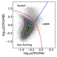
Figure 1: (a1)

Figure 2: (a2)

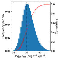
Figure 3: (b)

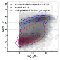
Figure 4: (c)

Figure 5: Panel (a1): The BPT diagram of the ionized gas regions identified from the MaNGA MPL-9. The red line from Kewley et al. (2001) and the blue line from Kewley et al. (2006) jointly divide the regions into three classes: star-forming regions (below the red line), Syeferts (above the two lines) and LINERs (above the red but below the blue line). The gray scale indicates the number density of the ionized gas regions in logarithm. The contours indicate the areas enclosing 30%, 60%, and 90% of the total sample. Panel (a2): It’s similar to panel (a1) but for [Oiii]$\;\lambda 5007$/$\rm H{\beta}$ versus [Nii]$\;\lambda 6583$/$\rm H{\alpha}$ diagram. The red line is from Kewley et al. (2001) and the blue line is from Kauffmann et al. (2003a). Regions above the red line are classified as AGN. Panel (b): The histogram shows the distribution of dust-corrected $\Sigma_{\rm H\alpha}$ for the final sample of ionized gas regions. The red line shows the cumulative distribution of the final sample. Panel (c): Diagram of $NUV-r$ color versus stellar mass. The red dashed contours show the distribution of the galaxies hosting the ionized gas regions in our final sample. The blue contours show the distribution of the parent MaNGA MPL-9 sample. The gray-scale distribution in the background is for a volume-limited sample of galaxies selected from the SDSS with $M_{\ast}>10^{9}M_{\odot}$ and $0.01<z<0.03$. See the text in Section 2.6.

2.6 Selection of ionized gas regions

For our analysis we further select a subset of the ionized gas regions with substantially higher S/N in both the stellar continuum and the relevant emission lines. Specifically, we require S/N$\;>5$ for the stellar continuum and the $\rm H{\alpha}$ and $\rm H{\beta}$ lines, and S/N$\;>3$ for the [Oii]$\;\lambda\lambda 3726,3729$, [Oiii]$\;\lambda 5007$, [Nii]$\;\lambda 6583$ and [Sii]$\;\lambda\lambda 6717,6731$. Furthermore, we exclude regions classified as AGN on the Baldwin-Phillips-Terlevich diagram (BPT; Baldwin et al., 1981). Figure 5 (panel (a1) and (a2)) displays the distribution of all the ionized gas regions in the planes of [Oiii]/$\rm H{\beta}$ versus [Sii]/$\rm H{\alpha}$ and [Oiii]/$\rm H{\beta}$ versus [Nii]/$\rm H{\alpha}$. The majority of the regions are located in the area classified as star-forming (or Hii). We first exclude all the regions that are classified as Seyfert on [Oiii]/$\rm H{\beta}$ versus [Sii]/$\rm H{\alpha}$ diagram. We also exclude the regions that are located within 3″ from their galactic center and are classified as either LINER on the [Oiii]/$\rm H{\beta}$ versus [Sii]/$\rm H{\alpha}$ diagram or AGN on the [Oiii]/$\rm H{\beta}$ versus [Nii]/$\rm H{\alpha}$ diagram.

These restrictions exclude about 45% of the ionized gas regions identified in Section 2.2, which results in a final sample of $\sim 2.7\times 10^{5}$ regions. Panel (b) of Figure 5 displays the histogram of $\Sigma_{\rm H\alpha}$ of the final sample. The distribution is peaked at around $10^{39}$$\rm erg\;s^{-1}\;kpc^{-2}$, as indicated by the vertical dashed line. As mentioned above, $\Sigma_{\rm H\alpha}$$\;\sim 10^{39}$$\rm erg\;s^{-1}\;kpc^{-2}$ can be used to effectively separate the low-$\Sigma_{\rm H\alpha}$ DIG regions from the high-$\Sigma_{\rm H\alpha}$ Hii regions. Thus, about 40% of our sample are DIG regions, while 60% are Hii regions. Panel (c) of Figure 5 displays the distribution of the galaxies that host our ionized gas regions in the $NUV-r$ versus $\log_{10}M_{\ast}$ plane, using data from the NSA (Blanton et al., 2011). For comparison, the distribution of the full sample of MaNGA MPL-9 is plotted as blue contours. We have also selected from the NSA a volume-limited sample consisting of $\sim 3.5\times 10^{4}$ galaxies with stellar mass $M_{\ast}>10^{9}M_{\odot}$ and with redshift in the range $0.01<z<0.03$. The distribution of this sample is plotted as the gray background in the figure. Overall, galaxies in the MaNGA MPL-9 follow the general population. The host galaxies of our ionized gas regions are mostly found as the ‘blue cloud’ population ($NUV-r<4$), with a considerable fraction at $M_{\ast}\gtrsim 10^{10}M_{\odot}$ extending to the green valley with $4<NUV<5$, and with a small fraction at the highest mass end ($M_{\ast}\sim 10^{11}M_{\odot}$) to the red sequence ($NUV-r>5$).

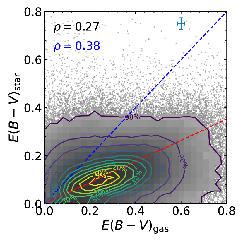
Figure 6: Distribution of the ionized gas regions in MaNGA galaxies on the diagram of $E(B-V)_{\rm star}$ versus $E(B-V)_{\rm gas}$. Contours of sample fraction are plotted and the contour levels are indicated. Individual ionized gas regions are plotted as small dots outside the 98% area. The Spearman rank correlation coefficients ($\rho$) are indicated for both the full sample (black) and the Hii regions (blue) selected by $\log_{10}$$\Sigma_{\rm H\alpha}$$\;>39$. The blue dashed line indicates the 1:1 relation, while the red dashed line represents $E(B-V)_{\rm star}$$\;=0.44$$E(B-V)_{\rm gas}$ which is the average relation of star-forming galaxies found by Calzetti et al. (2000). The typical uncertainties are shown in the upper right corner.

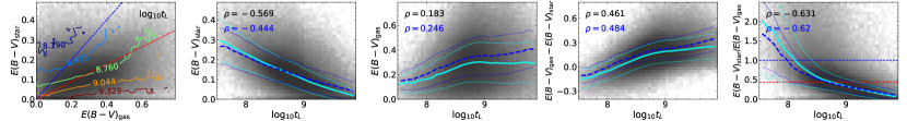
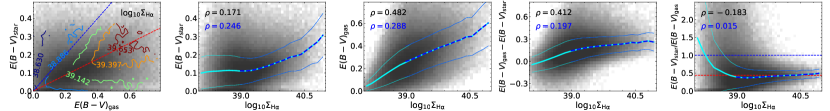
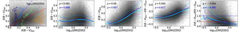
Figure 7: Correlations of $E(B-V)_{\rm star}$ and $E(B-V)_{\rm gas}$ on regional properties (panels from top to bottom): $\log_{10}$$t_{L}$, $\log_{10}$$\Sigma_{\rm H\alpha}$ and $\log_{10}$([Nii]/[Sii]). Panels in the left-most column show the diagram of $E(B-V)_{\rm star}$ versus $E(B-V)_{\rm gas}$ for all the ionized gas regions in our sample, with contours showing the distribution of the corresponding property. Panels from the second to the last column show the correlation of $E(B-V)_{\rm star}$, $E(B-V)_{\rm gas}$, $E(B-V)_{\rm gas}$$-$$E(B-V)_{\rm star}$ and $E(B-V)_{\rm star}$/$E(B-V)_{\rm gas}$ as functions of the property. The distribution of all the ionized gas regions are plotted as the gray-scale background in each panel, and the median relation and the 1$\sigma$ scatter are plotted as the cyan lines. The median relation and the 1$\sigma$ scatter of the subset of Hii regions selected by $\log_{10}$$\Sigma_{\rm H\alpha}$$\;>39$ are additionally plotted as the blue dashed lines. The Spearman rank correlation coefficients ($\rho$) for both the full sample (black) and the Hii regions (blue) are indicated.

3 Results

3.1 Correlations of dust attenuation with regional/global properties of galaxies

Figure 6 displays the distribution of all the ionized gas regions in our sample in the $E(B-V)_{\rm star}$ versus $E(B-V)_{\rm gas}$ plane. Overall, $E(B-V)_{\rm gas}$ spans a wider range than $E(B-V)_{\rm star}$, and there is a weak correlation between the two parameters. The Spearman rank correlation coefficients for both the full sample of ionized gas regions ($\rho=0.27$) and the subset of Hii regions of $\log_{10}$$\Sigma_{\rm H\alpha}$$\;>39$ ($\rho=0.38$) are quite low. For reference, we also plot the contours of constant sample fraction at levels ranging from 5% to 98%, as well as two linear relations: the 1:1 relation (blue dashed line) and $E(B-V)_{\rm star}$$\;=0.44$$E(B-V)_{\rm gas}$ (red dashed line), the previously found average relation of UV-bright starburst galaxies (e.g., Calzetti et al., 1994, 2000). The majority of the ionized gas regions are a bit below the red line, with large scatter. More interestingly, a significant population of the ionized gas regions is located above the 1:1 line, where the stellar attenuation is larger than the gas attenuation. A key goal of our study is to understand what drives the scatter in this diagram, particularly the bimodal distribution divided (roughly) by the 1:1 line.

We examine the dependence of $E(B-V)_{\rm star}$, $E(B-V)_{\rm gas}$, $E(B-V)_{\rm gas}-E(B-V)_{\rm star}$, and $E(B-V)_{\rm star}/E(B-V)_{\rm gas}$ on a variety of physical properties, both regional and global, in order to find the driving factor(s) for the overall distribution shown in Figure 6. We consider 13 regional properties: $\log_{10}$$\Sigma_{\rm H\alpha}$, $\log_{10}$$\rm{EW}_{H\alpha}$, sSFR, $\log_{10}$$\Sigma_{\ast}$, $\log_{10}$$t_{L}$, $\log_{10}$$t_{M}$, $Z_{L}$, $Z_{M}$, $D_{n}4000$, 12+$\log_{10}$(O/H), $\log_{10}$[Nii]/[Oii], $\log_{10}$[Oiii]/[Oii], $\log_{10}$[Nii]/[Sii], which are described in Section 2.4 and Section 2.5. In addition, three global properties are considered: total stellar mass ($M_{*}$), morphological type ($T$-type), and the $r$-band minor-to-major axial ratio ($b/a$). The measurements of $M_{*}$ and $b/a$ are taken from the NSA catalog (Blanton et al., 2005), and the estimates of $T$-type come from Domínguez Sánchez et al. (2018). A negative $T$-type usually indicates early-type morphology, while a positive $T$-type indicates late-type.

We find that, out of the 16 regional/global properties, dust attenuation shows the strongest correlation with the following three: $t_{L}$ for the stellar attenuation while $\Sigma_{\rm H\alpha}$ and [Nii]/[Sii] for the gas attenuation. Figure 7 shows the distribution of the ionized gas regions in the $E(B-V)_{\rm star}$ versus $E(B-V)_{\rm gas}$ space, color-coded by the three properties (panels in the leftmost column), as well as the correlation of four dust attenuation parameters ($E(B-V)_{\rm star}$, $E(B-V)_{\rm gas}$, and their difference and ratio) with the three properties (panels in the 2nd to 5th columns). In each of the correlation panels, the median relation and the 1$\sigma$ scatter around the median relation are plotted as solid cyan lines for all the ionized gas regions in our sample, and as blue dashed lines for the subset of Hii regions of $\log_{10}$$\Sigma_{\rm H\alpha}$$\;>39$. The Spearman rank correlation coefficients ($\rho$) are indicated for both the full sample and the subset. Results for the rest 13 properties, plotted in the same way, are presented in Appendix A.

By comparing the Spearman rank correlation coefficients, one can see that the stellar attenuation parameter $E(B-V)_{\rm star}$ shows the strongest (negative) correlation with stellar age. For the full sample, $\rho=-0.569$ for the luminosity-weighted age ($\log_{10}$$t_{L}$) and $\rho=-0.627$ for the mass-weighted age ($\log_{10}$$t_{M}$; see Figure 26). The stellar attenuation decreases with increasing $t_{L}$, from an average of $E(B-V)_{\rm star}$$\sim 0.3$ at $\log_{10}$($t_{L}$/yr)$\;\sim 7.5$ down to about zero at the oldest age, as can be seen from the first row of Figure 7. The correlation of $E(B-V)_{\rm star}$ with the other 12 properties is much weaker, with $|\rho|<0.2$ for all properties except the sSFR for which $\rho=0.339$. Similar results are obtained when the analysis is limited to Hii regions. These results strongly suggest that stellar age is the dominant parameter in driving the stellar attenuation, for both Hii and DIG regions. Compared to the mass-weighted stellar age ($\log_{10}$$t_{M}$), the luminosity-weighted age ($\log_{10}$$t_{L}$) shows a more linear correlation with stellar attenuation, although with a slightly smaller correlation coefficient. In addition, from the first row of Figure 7, one can see that the stellar age is positively correlated with the gas attenuation, although with a relatively small correlation coefficient ($\rho=0.183$). Consequently, $E(B-V)_{\rm gas}-E(B-V)_{\rm star}$ increases with $t_{L}$, while $E(B-V)_{\rm star}/E(B-V)_{\rm gas}$ decreases. Among all the properties and all the attenuation parameters, the strongest correlation is found between $E(B-V)_{\rm star}/E(B-V)_{\rm gas}$ and $\log_{10}$$t_{L}$, with $\rho=-0.631$. Thus, the driving role of $\log_{10}$$t_{L}$ in $E(B-V)_{\rm gas}-E(B-V)_{\rm star}$ and $E(B-V)_{\rm star}/E(B-V)_{\rm gas}$  comes mainly from the strong correlation between $E(B-V)_{\rm star}$ and $\log_{10}$$t_{L}$ , and the correlations of $E(B-V)_{\rm gas}-E(B-V)_{\rm star}$ and $E(B-V)_{\rm star}/E(B-V)_{\rm gas}$ with other properties are largely produced by this strong correlation with age.

Unlike $E(B-V)_{\rm star}$, the attenuation in gas, $E(B-V)_{\rm gas}$, shows strong correlations with multiple properties, including [Nii]/[Sii] ($\rho=0.58$) and $\Sigma_{\rm H\alpha}$ ($\rho=0.482$), as shown in Figure 7, and $\Sigma_{*}$ ($\rho=0.432$), as shown in Figure 26. From the second row of Figure 7, we can see that both $E(B-V)_{\rm star}$ and $E(B-V)_{\rm gas}$ are correlated with $\Sigma_{\rm H\alpha}$, but in different ways at both the high and low end of $\Sigma_{\rm H\alpha}$. For regions with $\log_{10}$$\Sigma_{\rm H\alpha}$$\;\gtrsim 39$, which are dominated by Hii regions, the two attenuation parameters behave quite similarly, showing positive correlations with $\Sigma_{\rm H\alpha}$. As a result, both their difference and ratio show a weak correlation with $\Sigma_{\rm H\alpha}$. The $E(B-V)_{\rm gas}-E(B-V)_{\rm star}$ increases slightly from $\sim 0.1$ mag at $\log_{10}$$\Sigma_{\rm H\alpha}$$\;=39$ up to $\sim 0.25$ mag at the highest $\Sigma_{\rm H\alpha}$. The $E(B-V)_{\rm star}/E(B-V)_{\rm gas}$ is almost constant at the value of 0.44 (Calzetti et al., 2000), ranging from $\sim 0.4$ at $\log_{10}$$\Sigma_{\rm H\alpha}$$\;=39$ to $\sim 0.5$ at $\log_{10}$$\Sigma_{\rm H\alpha}$$\;=41$, with small scatter. At $\log_{10}$$\Sigma_{\rm H\alpha}$$\;\lesssim 39$ where the regions are dominated by DIG, $E(B-V)_{\rm star}$ shows no obvious correlation with $\Sigma_{\rm H\alpha}$, with an average of $\sim 0.1$ mag and large scatter, while $E(B-V)_{\rm gas}$ rapidly increases with increasing $\Sigma_{\rm H\alpha}$. Consequently, the $E(B-V)_{\rm gas}-E(B-V)_{\rm star}$ increases and the $E(B-V)_{\rm star}/E(B-V)_{\rm gas}$ decreases as the $\Sigma_{\rm H\alpha}$ increases. At the lowest density, $\log_{10}$$\Sigma_{\rm H\alpha}$$\;\lesssim 38.5$, the stellar attenuation is stronger than the gas attenuation, mainly because of the small amount of dust in the gas as seen from the rapid decrease of $E(B-V)_{\rm gas}$ in the low-density end. The negative correlation of $E(B-V)_{\rm star}/E(B-V)_{\rm gas}$ with $\Sigma_{\rm H\alpha}$ has recently been discussed in depth in Lin & Kong (2020), based on an earlier sample of MaNGA. Our results show in addition that the correlation is essentially a result of the dichotomy of the intrinsic properties of the ionized gas regions, Hii regions and DIG regions, divided at $\Sigma_{\rm H\alpha}$$\;\sim 10^{39}$$\rm erg\;s^{-1}\;kpc^{-2}$ as suggested by Zhang et al. (2017). It is clear that Hii regions and DIG regions are distinct in terms of the dust attenuation, in the sense that Hii regions with higher $\Sigma_{\rm H\alpha}$ tend to be more dusty and have tighter correlation between the stellar and gas attenuation. It is thus necessary to consider the two types of regions separately when studying their dust properties.

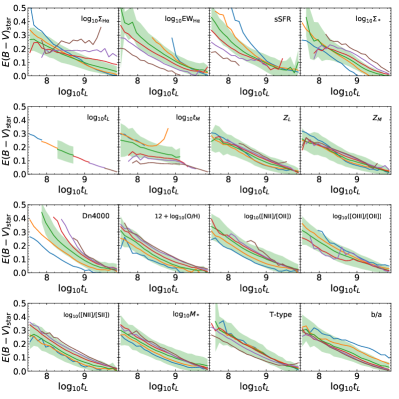
Figure 8: (a) $E(B-V)_{\rm star}$ versus $\log_{10}$$t_{L}$

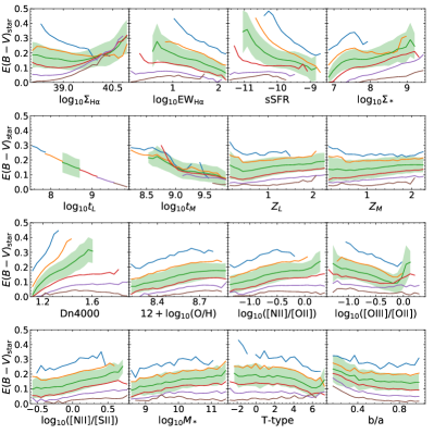
Figure 9: (b) $E(B-V)_{\rm star}$ versus regional/global properties

Figure 10: Panels (a): $E(B-V)_{\rm star}$ as a function of $\log_{10}$$t_{L}$. In each panel the different colors are for subsets of ionized gas regions selected by one of the 16 regional/global properties as indicated. The colors of cyan, orange, green, red, purple and brown correspond to subsets with increasing values of the property. For clarity, we only show the scatter of the green line as the scatters of other lines are comparable to that of the green line. Panels (b): $E(B-V)_{\rm star}$ as a function of regional and global properties. In each panel the different colors are for ionized gas regions in different intervals of $\log_{10}$$t_{L}$. The stellar age binning can be seen from the left-most panel in the second row.

The bottom row of Figure 7 shows the relationship between [Nii]/[Sii] and the four dust attenuation parameters. Both a strong correlation with the gas attenuation and the absence of correlation with the stellar attenuation can be clearly seen. For the gas attenuation, the strong correlation is seen only when [Nii]/[Sii] exceeds $\sim-0.2$. In addition, noticeable correlations between gas attenuation and the gas-phase metallicity or related parameters are also found: $\rho=0.445$ for $12+\log_{10}(\rm O/H)$ and $\rho=-0.461$ for [Oiii]/[Oii] (see Figure 26), which may share the same origin with the correlation with $\Sigma_{*}$ given the well-known mass-metallicity relation (Tremonti et al., 2004). Similar to [Nii]/[Sii], the [Oiii]/[Oii] also shows no correlation with the stellar attenuation, but a strong correlation with the gas attenuation (see Figure 26). Both [Nii]/[Sii] and [Oiii]/[Oii] have been used as indicators of the ionization level of gas (Dopita et al., 2013; Lin & Kong, 2020). In the ionization model of spherical Hii regions from Dopita et al. (2013), the line ratio of [Oiii]/[Oii] increases as the ionization parameter ($q$) increases, when the gas-phase metallicity diagnostics (e.g. [Nii]/[Oii]) are fixed. Based on the same models and the MaNGA data, Lin & Kong (2020) found the line ratio [Nii]/[Sii] to be sensitive to both the gas-phase metallicity and the ionization parameter, with smaller values of [Nii]/[Sii] in metal-poorer regions at fixed $q$. Note that $E(B-V)_{\rm gas}$ is also moderately correlated with $D_{n}4000$ ($\rho=0.386$) and $\log_{10}$$M_{*}$ ($\rho=0.459$). The former may be related to its correlation with stellar age as mentioned above, while the latter may be a result of its correlation with $\Sigma_{*}$.

In conclusion, we find that the stellar attenuation is mostly driven by stellar age, while the gas attenuation is most strongly related to $\Sigma_{\rm H\alpha}$, [Nii]/[Sii] and [Oiii]/[Oii]. In the latter case, $\Sigma_{\rm H\alpha}$ divides ionized gas regions into two distinct types, DIG regions and Hii regions, and [Nii]/[Sii] and [Oiii]/[Oii] are indicators of the gas-phase metallicity and ionization level. For the stellar-to-gas attenuation ratio (or difference), both stellar age and $\Sigma_{\rm H\alpha}$ play important roles. In the following subsections, we will discuss these findings further. We will focus on the stellar age versus stellar attenuation relation in Section 3.2, the role of $\Sigma_{\rm H\alpha}$, [Nii]/[Sii] and [Oiii]/[Oii] for the gas attenuation in Section 3.3, and the joint role of $\log_{10}$$t_{L}$ and $\Sigma_{\rm H\alpha}$ for the stellar-to-gas attenuation ratio in Section 3.4.

3.2 The role of stellar age in driving stellar attenuation

In this subsection we concentrate on $t_{L}$, which has the strongest correlation with $E(B-V)_{\rm star}$, when compared to any other regional/global properties. This implies the potential dominant role of the stellar age in driving the dust attenuation parameters. In order to test this hypothesis, we divide the ionized gas regions into different intervals of $\log_{10}$$t_{L}$, and examine the correlations of $E(B-V)_{\rm star}$ with other regional/global properties. Similarly, for a given regional/global property, we divide the ionized regions into intervals of the property, and examine the correlations of the dust attenuation parameters with $\log_{10}$$t_{L}$. The results are shown in Figure 10.

Panels (a) of Figure 10 show the correlation of $E(B-V)_{\rm star}$ with $\log_{10}$$t_{L}$, but for the subsets of ionized gas regions selected by each of the regional/global properties. Panels (b) show the correlation of $E(B-V)_{\rm star}$ with different regional/global properties, but for the subsets of ionized gas regions selected by $\log_{10}$$t_{L}$. In most cases, $E(B-V)_{\rm star}$ shows tight correlations with $\log_{10}$$t_{L}$ even when the sample is limited to a narrow range of a specific property, as can be seen from panels (a), while $E(B-V)_{\rm star}$ shows no or rather weak dependence on all other properties once the stellar age is limited to a narrow range, as shown in panels (b). This result reinforces the conclusion from the previous subsection that the stellar attenuation is predominantly driven by the stellar age.

One can identify two subsets of the ionized gas regions in which residual correlations are clearly seen. The subset, which consists of the regions with both high $\rm H{\alpha}$ surface brightness ($\Sigma_{\rm H\alpha}$$\;\gtrsim 10^{39}$$\rm erg\;s^{-1}\;kpc^{-2}$) and old stellar ages ($t_{L}$$\;\gtrsim 1$Gyr), shows that the $E(B-V)_{\rm star}$ is more strongly correlated with $\Sigma_{\rm H\alpha}$ than with $\log_{10}$$t_{L}$. This can be seen from the top-left panel in both panels (a) and (b) of the figure. The second subset, consisting of regions with very young ages (with $t_{L}$ less than a few $\times 10^{8}$yr), shows residual correlations with $D_{n}4000$ (as well as with $\rm{EW}_{H\alpha}$ and sSFR) at fixed $\log_{10}$$t_{L}$.

We have done the same analysis for $E(B-V)_{\rm gas}-E(B-V)_{\rm star}$ and $E(B-V)_{\rm star}/E(B-V)_{\rm gas}$, and the results are presented in Appendix B. We see that the stellar age is correlated with both $E(B-V)_{\rm gas}-E(B-V)_{\rm star}$ and $E(B-V)_{\rm star}/E(B-V)_{\rm gas}$ in most cases when other properties are fixed, while at fixed $\log_{10}$$t_{L}$ no strong correlation is seen between either of the attenuation parameters and other properties. These behaviors can be attributed largely to the correlation between $E(B-V)_{\rm star}$ and $\log_{10}$$t_{L}$, as shown in Figure 10.

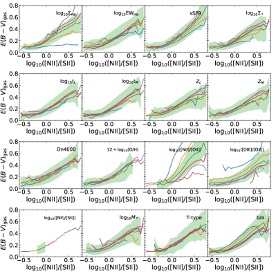
Figure 11: (a) $E(B-V)_{\rm gas}$ versus $\log_{10}$([Nii]/[Sii])

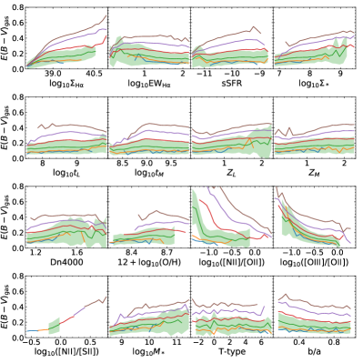
Figure 12: (b) $E(B-V)_{\rm gas}$ versus regional/global properties

Figure 13: $E(B-V)_{\rm gas}$ as function of $\log_{10}$([Nii]/[Sii]) for subsets of ionized gas regions selected by each of the 16 regional/global properties as indicated (panels a), and as functions of regional/global properties for subsets of ionized gas regions selected by $\log_{10}$([Nii]/[Sii]) (panels b). Symbols/lines are the same as in Figure 10.

3.3 The role of $\Sigma_{\rm H\alpha}$, [Nii]/[Sii] and [Oiii]/[Oii] in driving gas attenuation

Similarly, we have compared the dependence of $E(B-V)_{\rm gas}$ on $\Sigma_{\rm H\alpha}$, [Nii]/[Sii] and [Oiii]/[Oii] with that on other regional/global properties. We find that, among the three properties, [Nii]/[Sii] shows stronger correlations with $E(B-V)_{\rm gas}$ than both $\Sigma_{\rm H\alpha}$ and [Oiii]/[Oii] when other properties are limited to a narrow range. This is consistent with the fact that the highest correlation efficient is between $E(B-V)_{\rm gas}$ and [Nii]/[Sii] (see Section 3.1). We therefore only show the results for [Nii]/[Sii] in Figure 13, and present the results for $\Sigma_{\rm H\alpha}$ and [Oiii]/[Oii] in Appendix B.

As can be seen from Figure 13, the gas attenuation is positively correlated with [Nii]/[Sii] when other properties are fixed, but this is true only for Hii regions with $\Sigma_{\rm H\alpha}$$\;\gtrsim 10^{39}$$\rm erg\;s^{-1}\;kpc^{-2}$. This result echoes the $\Sigma_{\rm H\alpha}$ dichotomy as discussed above. For DIG regions with lower $\Sigma_{\rm H\alpha}$, the gas attenuation shows weak dependence on [Nii]/[Sii] (see the top-left panel of panels (a)), and strong dependence on $\Sigma_{\rm H\alpha}$ when [Nii]/[Sii] is fixed (see the top-left panel of panels (b)). Apparently, [Nii]/[Sii] plays a dominant role for Hii regions, showing strong correlations with $E(B-V)_{\rm gas}$ in almost all cases when the regional/global properties, including $\Sigma_{\rm H\alpha}$  are fixed (panels (a)). No residual correlation of $E(B-V)_{\rm gas}$ is seen for most of the regional/global properties if $\log_{10}$([Nii]/[Sii]) is fixed (panels (b)). Two properties, [Nii]/[Oii] and [Oiii]/[Oii], show residual correlations with $E(B-V)_{\rm gas}$ at fixed $\log_{10}$([Nii]/[Sii]). This probably is not surprising. As found in Lin & Kong (2020), [Nii]/[Sii] is sensitive to both gas-phase metallicity and the ionized level of the gas, and thus expected to correlate with both [Nii]/[Oii]  which is a metallicity indicator, and [Oiii]/[Oii]  which is an indicator of the ionized level.

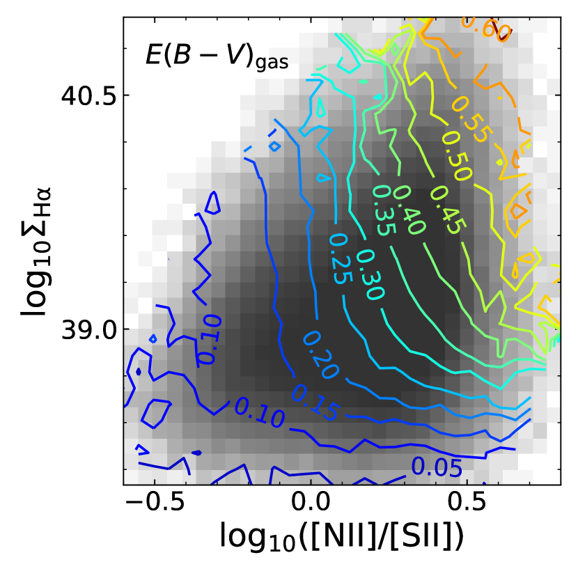
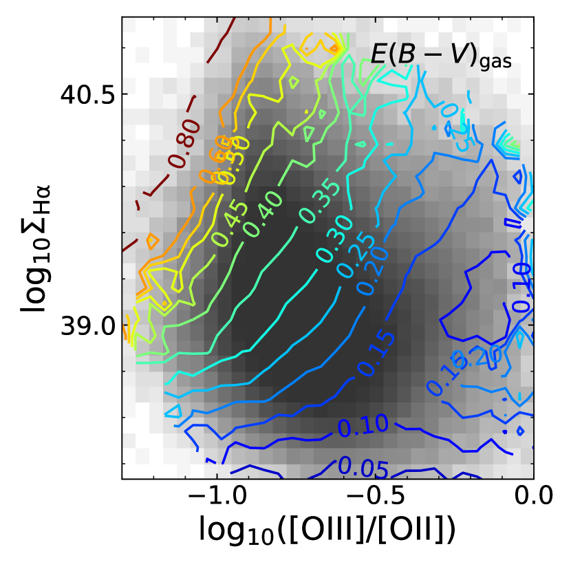
Figure 14: Distribution of all the ionized gas regions on the plane of $\log_{10}$$\Sigma_{\rm H\alpha}$ versus $\log_{10}$([Nii]/[Sii]) (left panel) and the plane of $\log_{10}$$\Sigma_{\rm H\alpha}$ versus $\log_{10}$([Oiii]/[Oii]) (right panel) are plotted as the gray-scale background, while contours of $E(B-V)_{\rm gas}$ are plotted in the colored lines with contour levels being indicated.

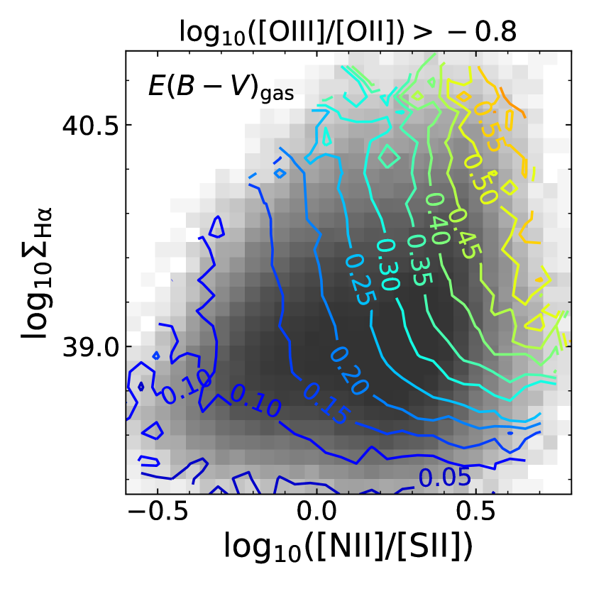
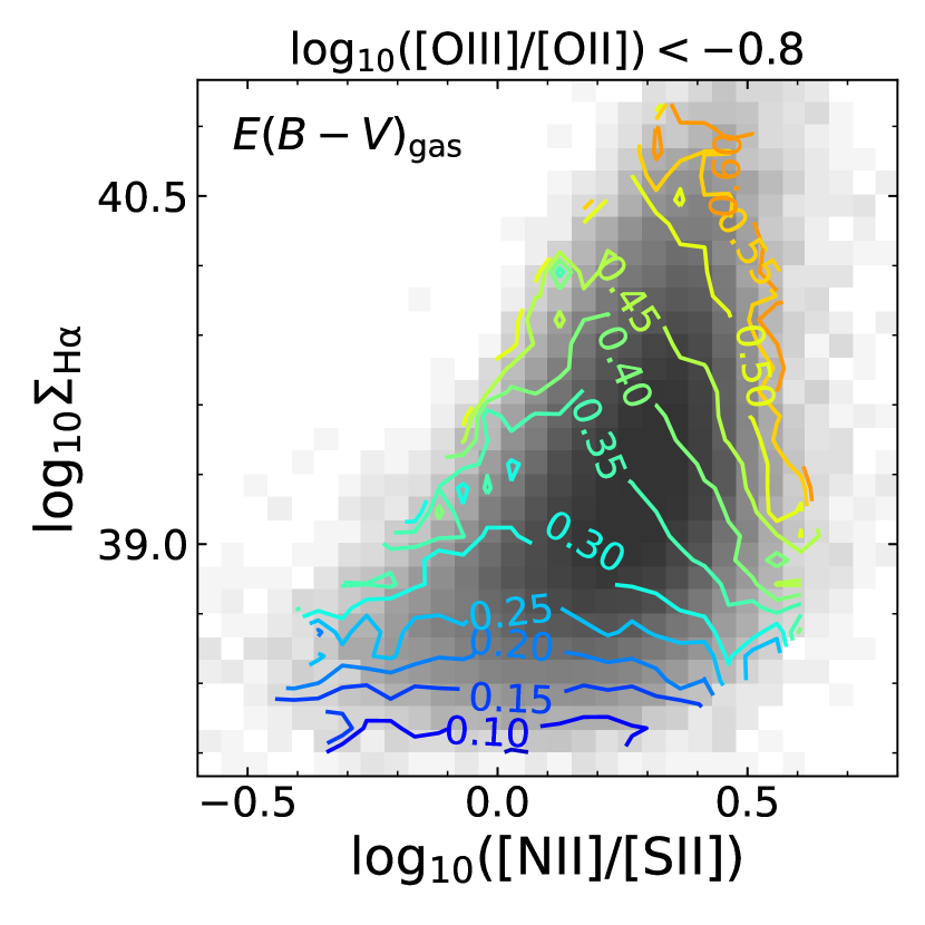
Figure 15: Distribution on the plane of $\log_{10}$$\Sigma_{\rm H\alpha}$ versus $\log_{10}$([Nii]/[Sii]) for ionized gas regions with $\log_{10}$([Oiii]/[Oii])$\;>-0.8$ (left panel) and those with $\log_{10}$([Oiii]/[Oii])$\;<-0.8$ (right panel). Symbols/lines are the same as in Figure 14.

Figure 13 suggests that the $E(B-V)_{\rm gas}$ is determined mainly by two parameters: $\Sigma_{\rm H\alpha}$ for DIG regions with low $\Sigma_{\rm H\alpha}$, and [Nii]/[Sii] for Hii regions with high $\Sigma_{\rm H\alpha}$. This finding is more clearly seen in Figure 14 (left panel) where we show the contours of $E(B-V)_{\rm gas}$ in the diagram of $\log_{10}$$\Sigma_{\rm H\alpha}$ versus $\log_{10}$([Nii]/[Sii]). Below $\log_{10}$$\Sigma_{\rm H\alpha}$$\;\sim 39$, the contours are almost horizontal, and so the change of $E(B-V)_{\rm gas}$ is mainly driven by $\Sigma_{\rm H\alpha}$. Above $\log_{10}$$\Sigma_{\rm H\alpha}$$\;\sim 39$, in contrast, the contours are largely vertical, indicating that $E(B-V)_{\rm gas}$ is driven mainly by $\log_{10}$([Nii]/[Sii]). In the right panel of the same figure, we show the contours of $E(B-V)_{\rm gas}$ in the $\log_{10}$$\Sigma_{\rm H\alpha}$ versus $\log_{10}$([Oiii]/[Oii]) plane. Below $\log_{10}$$\Sigma_{\rm H\alpha}$$\;\sim 39$, again, the $E(B-V)_{\rm gas}$ is mainly driven by $\Sigma_{\rm H\alpha}$  with no correlation with [Oiii]/[Oii]. At higher $\Sigma_{\rm H\alpha}$, the contours are inclined, indicating that neither $\Sigma_{\rm H\alpha}$ nor [Oiii]/[Oii] alone can dominate in the $E(B-V)_{\rm gas}$. At fixed $\Sigma_{\rm H\alpha}$, the correlation of $E(B-V)_{\rm gas}$ with [Oiii]/[Oii] appears to be weaker in regions with $\log_{10}$([Oiii]/[Oii])$\;\gtrsim-0.8$ than in lower ionization regions.

Figure 15 displays the $\Sigma_{\rm H\alpha}$–[Nii]/[Sii] relation again, but separately for high and low ionization regions divided at $\log_{10}$([Oiii]/[Oii])$\;=-0.8$. The high ionization regions (left panel) cover almost the full range in the diagram, and the contours in Hii regions (high $\Sigma_{\rm H\alpha}$) and with high [Nii]/[Sii] (high metallicity) become more vertical when compared to those for the full sample, suggesting that the diagnostic of [Oiii]/[Oii] in these regions may be negligible. This is consistent with the weak correlation of $E(B-V)_{\rm gas}$ with [Oiii]/[Oii] at $\log_{10}$([Oiii]/[Oii])$\;\gtrsim-0.8$ seen in the right panel of Figure 14. Low ionization regions (right panel) are distributed differently: they are either DIG regions spanning all the range of [Nii]/[Sii], or limited to Hii regions of high [Nii]/[Sii]. In the latter case the $E(B-V)_{\rm gas}$ depends jointly on $\Sigma_{\rm H\alpha}$ and [Nii]/[Sii], as indicated by the inclined contours. Apparently, the diagnostic of [Oiii]/[Oii] cannot be neglected for low ionization Hii regions.

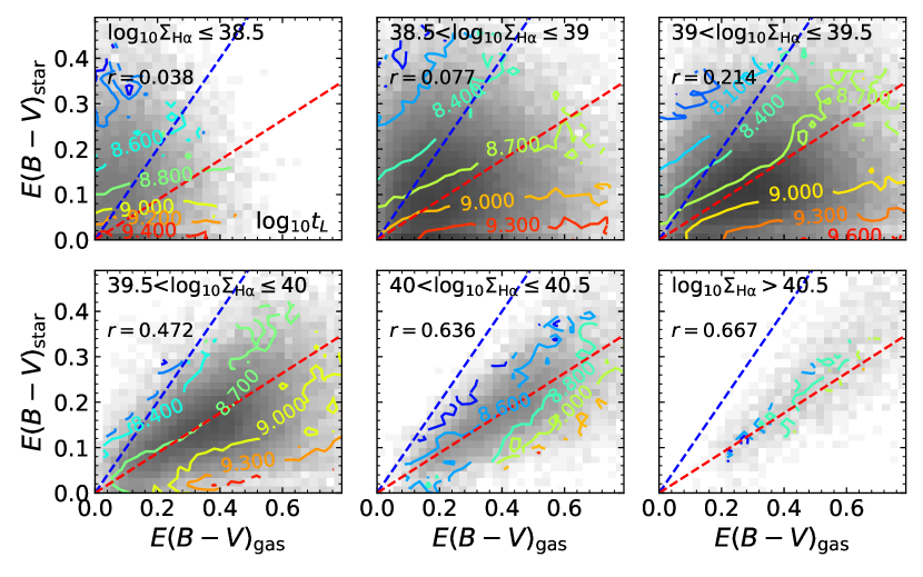
Figure 16: $E(B-V)_{\rm star}$ versus $E(B-V)_{\rm gas}$ in different intervals of $\Sigma_{\rm H\alpha}$. The colored lines are the contours of $\log_{10}$$t_{L}$ as indicated, and the gray-scale background shows the number density distribution of the ionized gas regions in each $\Sigma_{\rm H\alpha}$ bin. The blue dashed line is the 1:1 relation and the red dashed line represents the relation of $E(B-V)_{\rm star}$$\;=0.44$$E(B-V)_{\rm gas}$. The Pearson linear correlation coefficient ($r$) between the two attenuations is indicated in each panel.

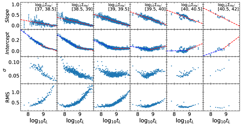
Figure 17: Upper two rows show the slope and intercept of the relation in Equation 3 as a function of $\log_{10}$$t_{L}$, for different intervals of $\log_{10}$$\Sigma_{\rm H\alpha}$. In each panel, the dashed red/blue lines are the best-fit model. The third row shows the standard deviation of ionized gas regions around the best-fit relation ($\sigma$), while the bottom row shows the rms of the relative difference of the ionized gas regions from the best-fit relation ($\sigma/$best-fit). See text for details.

3.4 Dependence of $E(B-V)_{\rm star}/E(B-V)_{\rm gas}$ on both $\Sigma_{\rm H\alpha}$ and $t_{L}$

In this subsection we focus on the stellar-to-gas attenuation ratio, $E(B-V)_{\rm star}/E(B-V)_{\rm gas}$. The analysis so far has revealed that the stellar age is the property most strongly correlated with $E(B-V)_{\rm star}/E(B-V)_{\rm gas}$ (see Figure 7), and that the $\Sigma_{\rm H\alpha}$ plays an important role as well. The residual dependence on $\Sigma_{\rm H\alpha}$ at fixed $\log_{10}$$t_{L}$ can largely be attributed to the dichotomy of the ionized gas regions. Thus, all the regions can be well divided into Hii regions with high $\Sigma_{\rm H\alpha}$ and DIG regions with low $\Sigma_{\rm H\alpha}$. In this subsection we study the dependence of $E(B-V)_{\rm star}/E(B-V)_{\rm gas}$ on $\Sigma_{\rm H\alpha}$ and $t_{L}$ jointly.

Figure 16 shows the distribution of the ionized regions in the $E(B-V)_{\rm star}$ versus $E(B-V)_{\rm gas}$ plane, but for six successive, non-overlapping intervals of $\log_{10}$$\Sigma_{\rm H\alpha}$. In each $\log_{10}$$\Sigma_{\rm H\alpha}$ interval, the distribution of the ionized gas regions is plotted in gray scales, overlaid with colored contours of $\log_{10}$$t_{L}$. The Pearson linear correlation coefficient is also indicated in each panel. For DIG regions with $\log_{10}$$\Sigma_{\rm H\alpha}$$\;\lesssim 39$, the correlation coefficient is close to zero, indicative of no correlation. At fixed $E(B-V)_{\rm gas}$, $E(B-V)_{\rm star}$ spans the full range from zero up to $\sim 0.5$ mag, while $E(B-V)_{\rm gas}$ is limited to relatively low values with the upper limit increasing from $\sim 0.2$ mag at $\log_{10}$$\Sigma_{\rm H\alpha}$$\;\leq 38.5$ to $\sim 0.6$ mag at $38.5<\;$$\log_{10}$$\Sigma_{\rm H\alpha}$$\;\leq 39$. For Hii regions, as $\Sigma_{\rm H\alpha}$ increases, the correlation between the two $E(B-V)$ measurements becomes more and more evident and the scatter decreases steadily. The average relation of the Hii regions follows the relation $E(B-V)_{\rm star}$$\;=0.44$$E(B-V)_{\rm gas}$, which is indicated by the red dashed line in each panel. When $\log_{10}$$\Sigma_{\rm H\alpha}$ exceeds $\sim 39.5$, almost all the regions fall below the 1:1 relation.

When $\log_{10}$$t_{L}$ is fixed, $E(B-V)_{\rm star}$ is linearly correlated with $E(B-V)_{\rm gas}$, and this is true in all the different $\log_{10}$$\Sigma_{\rm H\alpha}$ intervals, although the slope and intercept of the linear relation vary with both $\log_{10}$$t_{L}$ and $\log_{10}$$\Sigma_{\rm H\alpha}$. To quantify the joint dependence on $\log_{10}$$\Sigma_{\rm H\alpha}$ and $\log_{10}$$t_{L}$, we perform a linear fitting to the relation between $E(B-V)_{\rm star}$ and $E(B-V)_{\rm gas}$ for given $\log_{10}$$t_{L}$ and $\log_{10}$$\Sigma_{\rm H\alpha}$. For each $\log_{10}$$\Sigma_{\rm H\alpha}$ bin, the ionized gas regions are sorted by increasing $\log_{10}$$t_{L}$, and are divided into a number of $\log_{10}$$t_{L}$ bins by requiring each bin to contain 200 ionized gas regions. A linear relation is obtained by fitting the following equation to the data in each bin:

$$\mbox{{$E(B-V)_{\rm star}$}}=Slope\times\mbox{$E(B-V)_{\rm gas}$}+Intercept.$$ (3)

The upper two panels in Figure 17 show the best-fit $Slope$ and $Intercept$ as functions of $\log_{10}$$t_{L}$, for different $\log_{10}$$\Sigma_{\rm H\alpha}$ bins. Overall, the relations are quite flat at the lowest $\Sigma_{\rm H\alpha}$ and the highest $t_{L}$, with a slope close to zero for regions with $\log_{10}$$\Sigma_{\rm H\alpha}$$\;<38.5$ and $t_{L}$ older than a few Gyr. The slope increases with $\Sigma_{\rm H\alpha}$ at fixed $t_{L}$, and decreases with $t_{L}$ at fixed $\Sigma_{\rm H\alpha}$. The intercept behaves differently for young regions with $t_{L}$$\;\lesssim 1$Gyr and old regions with higher $t_{L}$. For the young regions, the intercept decreases with both $t_{L}$ and $\Sigma_{\rm H\alpha}$, while for the old regions, the intercept decreases with $t_{L}$ in DIG regions, and increases with $t_{L}$ in Hii regions. For DIG regions, the small $Slope$ suggests a poor correlation between $E(B-V)_{\rm star}$ and $E(B-V)_{\rm gas}$. In Hii regions, the $Intercept$ is relatively small, close to zero in Hii regions with $\log_{10}$$\Sigma_{\rm H\alpha}$$\;>39.5$. The $Slope$ is thus approximately equal to $E(B-V)_{\rm star}/E(B-V)_{\rm gas}$ for these Hii regions, with a value comparable to the average of $E(B-V)_{\rm star}/E(B-V)_{\rm gas}$$\;\approx 0.44$, but varying with both $t_{L}$ and $\Sigma_{\rm H\alpha}$.

The lower two panels of Figure 17 show the standard deviation of the ionized gas regions around the best-fit relation, and the rms of their relative difference from the best-fit relation. The scatter of the ionized regions around the $E(B-V)_{\rm star}$ versus $E(B-V)_{\rm gas}$ relations depends on $\Sigma_{\rm H\alpha}$ and $t_{L}$ in a way similar to the dependence of the intercept on these two parameters. Overall, the scatter is smaller than 0.1 mag in all cases, and is relatively large for DIG regions of young ages ($\Sigma_{\rm H\alpha}$$\;\lesssim 10^{39}$$\rm erg\;s^{-1}\;kpc^{-2}$ and $t_{L}$$\;\lesssim 1$Gyr) and for high-$\Sigma_{\rm H\alpha}$ Hii regions of old ages ($\Sigma_{\rm H\alpha}$$\;\gtrsim 10^{40}$$\rm erg\;s^{-1}\;kpc^{-2}$ and $t_{L}$$\;\gtrsim 1$Gyr), ranging from 0.05 mag to 0.1 mag. The rms of the relative difference from the best-fit relations decreases with increasing $\Sigma_{\rm H\alpha}$, and it is smaller than 50% at ages younger than $\sim 1$Gyr with weak dependence on $t_{L}$. At older ages, the rms is only 20-30% at the highest $\Sigma_{\rm H\alpha}$ ($>10^{40}$$\rm erg\;s^{-1}\;kpc^{-2}$), but increases rapidly towards lower $\Sigma_{\rm H\alpha}$. The large rms at the low $\Sigma_{\rm H\alpha}$ again reflects the poor correlations between the stellar and gas attenuation in the DIG regions.

Table 1: Best-fit coefficients in Equation 4 and Equation 7 which describe the slope and intercept of the stellar-to-gas attenuation linear relation as a function of luminosity-weighted stellar age.

$\log_{10}$$\Sigma_{\rm H\alpha}$	$a_{0}$	$b_{0}$	$a_{1}$	$b_{1}$	$a_{2}$	$b_{2}$
(, 38.5]	-0.130	1.253	-0.211	1.968	-0.101	0.996
(38.5, 39.0]	-0.174	1.692	-0.168	1.553	-0.058	0.582
(39.0, 39.5]	-0.234	2.286	-0.110	1.012	0.0006	0.041
(39.5, 40.0]	-0.257	2.576	-0.049	0.452	0.062	-0.520
(40.0, 40.5]	-0.271	2.766	0.007	-0.052	0.118	-1.024
(40.5, ]	-0.360	3.527	0.097	-0.812	0.207	-1.783

As can be seen from Figure 17, both $Slope$ and $Intercept$ depend on $\log_{10}$$t_{L}$ in a rather simple way. For a given $\Sigma_{\rm H\alpha}$ range, we model $Slope$ and $Intercept$ as function of $\log_{10}$$t_{L}$ using

$$Slope=a_{0}\times\log_{10}t_{L}+b_{0},$$ (4)

and

$$Intercept=\left\{\begin{array}[]{ll}a_{1}\times\log_{10}t_{L}+b_{1},\mbox{if}\;\log_{10}t_{L}\leq 8.8\\ a_{2}\times\log_{10}t_{L}+b_{2},\mbox{if}\;\log_{10}t_{L}>8.8\end{array}\right.$$ (7)

The best-fit relations are plotted in Figure 17 as the dashed lines, and the best-fit values of $a_{0}$, $b_{0}$, $a_{1}$, $b_{1}$, $a_{2}$ and $b_{2}$ are listed in Table 1 for the different intervals of $\Sigma_{\rm H\alpha}$.

4 Discussion

4.1 Comparison with previous MaNGA-based studies

Recently, Lin & Kong (2020) and Greener et al. (2020) have used the MaNGA data to study the dust attenuation in nearby galaxies. In this subsection we compare our work with both studies. We note that, in a recent study based on MaNGA, Riffel et al. (2021) also examined the correlation between $E(B-V)_{\rm star}$ and $E(B-V)_{\rm gas}$, but focusing on AGN host galaxies and a control sample of star-forming galaxies. Here we will not make comparisons with this study, given the difference in sample selection.

4.1.1 Comparison with Lin & Kong (2020)

Lin & Kong (2020) used the dust attenuation parameters and spectroscopic properties from the MaNGA value-added catalog produced by applying the Pipe3D pipeline (Sánchez et al., 2018) to the SDSS DR15 that contains $\sim 4,800$ datacubes from MaNGA. Pipe3D performed spatial binning for each datacube and fitted the binned spectra with a set of simple stellar population models base (González Delgado et al., 2005; Vazdekis et al., 2010; Cid Fernandes et al., 2013). The dust attenuation curve of Cardelli et al. (1989) and a selective extinction of $R_{V}=3.1$ were assumed, and a stellar attenuation was determined as one of the free parameters in the spectral fitting.

The authors examined the correlation between $E(B-V)_{\rm star}$ and $E(B-V)_{\rm gas}$, and the dependence on a variety of galaxy properties, both regional and global. In particular, they found that both the Pearson and Spearman rank correlation coefficients increase rapidly with $\log_{10}$$\Sigma_{\rm H\alpha}$, from $<0.1$ at $\log_{10}$$\Sigma_{\rm H\alpha}$$\;<39$ up to $\sim 0.8$ at $\log_{10}$$\Sigma_{\rm H\alpha}$$\;>40.5$ (see their figure 2). This dependence is also seen in our results, e.g. in Figure 16. We further find that the scatter in the relation between $E(B-V)_{\rm star}$ and $E(B-V)_{\rm gas}$ at fixed $\Sigma_{\rm H\alpha}$ can well be explained by the stellar age, which can also be seen from Figure 16. Once limited to a narrow range of $\log_{10}$$t_{L}$, the two attenuation parameters are linearly correlated, although the slope, intercept and scatter of the relation vary with $\Sigma_{\rm H\alpha}$ and $t_{L}$. We show that the variations can be described quantitatively by simple functions (see Figure 17 and Table 1).

Lin & Kong (2020) payed particular attention to $E(B-V)_{\rm star}/E(B-V)_{\rm gas}$, finding it to be larger in DIG regions than in Hii regions, which is also found from our data (see Figure 7). According to the Spearman rank correlation analysis, they found that $E(B-V)_{\rm star}$/$E(B-V)_{\rm gas}$ is the most strongly correlated with $\log_{10}$([Nii]/[Sii]), with a correlation coefficient close to $\rho=-0.5$, and is the least strongly correlated with $D_{n}4000$, with $\rho\sim-0.1$ (see their figure 3). In contrast, we find that, among other properties, the luminosity-weighted stellar age $t_{L}$ is the property that shows the strongest correlation with $E(B-V)_{\rm star}$/$E(B-V)_{\rm gas}$, with $\rho=-0.63$ (see Figure 7). The Spearman correlation coefficient is $\rho=-0.38$ between $E(B-V)_{\rm star}$/$E(B-V)_{\rm gas}$ and $D_{n}4000$, not as weak as found in Lin & Kong (2020). The different correlation coefficient for $D_{n}4000$ may be attributed to the different data products used in the two studies. In fact, we have repeated the analysis of the correlation between $E(B-V)_{\rm star}$/$E(B-V)_{\rm gas}$ and $D_{n}4000$ using measurements from the Pipe3D VAC, and found a similarly weak correlation.

In Section 3.1 we have discussed the dominant role of the stellar age in driving $E(B-V)_{\rm star}$, as well as its difference and ratio relative to $E(B-V)_{\rm gas}$. This analysis was missing in Lin & Kong (2020) for two reasons. First, the authors did not consider the stellar age directly, but adopted $D_{n}4000$ as an indicator of it. The $D_{n}4000$ is indeed a good indicator of stellar age, but sensitive only to populations younger than 1-2Gyr (Bruzual & Charlot, 2003; Kauffmann et al., 2003b). Second, our measurements of $E(B-V)_{\rm star}$ are more reliable and accurate than in previous studies, because we use the new technique of measuring stellar attenuation developed in Paper I. As shown in Appendix B of Paper I, our method can obtain $E(B-V)_{\rm star}$ before the stellar population is modeled, thus significantly alleviating the degeneracy between dust attenuation and stellar population properties, such as stellar age and metallicity. We have used data from the Pipe3D VAC and found the Spearman rank correlation coefficient to be $\rho=-0.3$ between $E(B-V)_{\rm star}/E(B-V)_{\rm gas}$ and $\log_{10}$$t_{L}$. Thus, the dominant role of the stellar age would be missed in our analysis if the stellar attenuation and age measurements were not improved substantially.

We find that the Spearman correlation coefficient between $E(B-V)_{\rm star}/E(B-V)_{\rm gas}$ and [Nii]/[Sii] is $\rho=-0.36$ (see Figure 7), weaker than the coefficient of $\rho\sim-0.5$ found in Lin & Kong (2020). Again, using the Pipe3D data we obtain $\rho=-0.49$, in good agreement with their result. Assuming the relevant emission lines are measured reasonably well in both studies, we conclude that the different correlation coefficients for the relation of $E(B-V)_{\rm star}/E(B-V)_{\rm gas}$with [Nii]/[Sii] are caused mainly by the different measurements of $E(B-V)_{\rm star}$. Our $E(B-V)_{\rm star}$ measurements are expected to be more reliable for the reasons mentioned above. On the other hand, we find that [Nii]/[Sii] is indeed one of the dominant parameters for $E(B-V)_{\rm gas}$, as discussed in Section 3.1, and drives the gas attenuation in Hii regions. Furthermore, we confirm the finding of Lin & Kong (2020) that the ionization level of the gas as indicated by [Oiii]/[Oii] cannot be simply neglected, and we find that this parameter needs to be considered only in Hii regions with low ionization, $\log_{10}$([Oiii]/[Oii])$\;\lesssim-0.8$.

To conclude, comparing with Lin & Kong (2020), we confirm the following results:

• The relation between $E(B-V)_{\rm star}$ and $E(B-V)_{\rm gas}$ is stronger for more active Hii regions;

• Local physical properties such as metallicity and ionization level play important roles in determining the dust attenuation.

In addition we obtain the following new results:

• Stellar age is the driving factor for $E(B-V)_{\rm star}$, and consequently for $E(B-V)_{\rm gas}-E(B-V)_{\rm star}$ and $E(B-V)_{\rm star}/E(B-V)_{\rm gas}$;

• At fixed $\Sigma_{\rm H\alpha}$, the stellar age is linearly correlated with $E(B-V)_{\rm star}/E(B-V)_{\rm gas}$ at all ages;

• Gas-phase metallicity and ionization level are important, but only for the attenuation in $E(B-V)_{\rm gas}$.

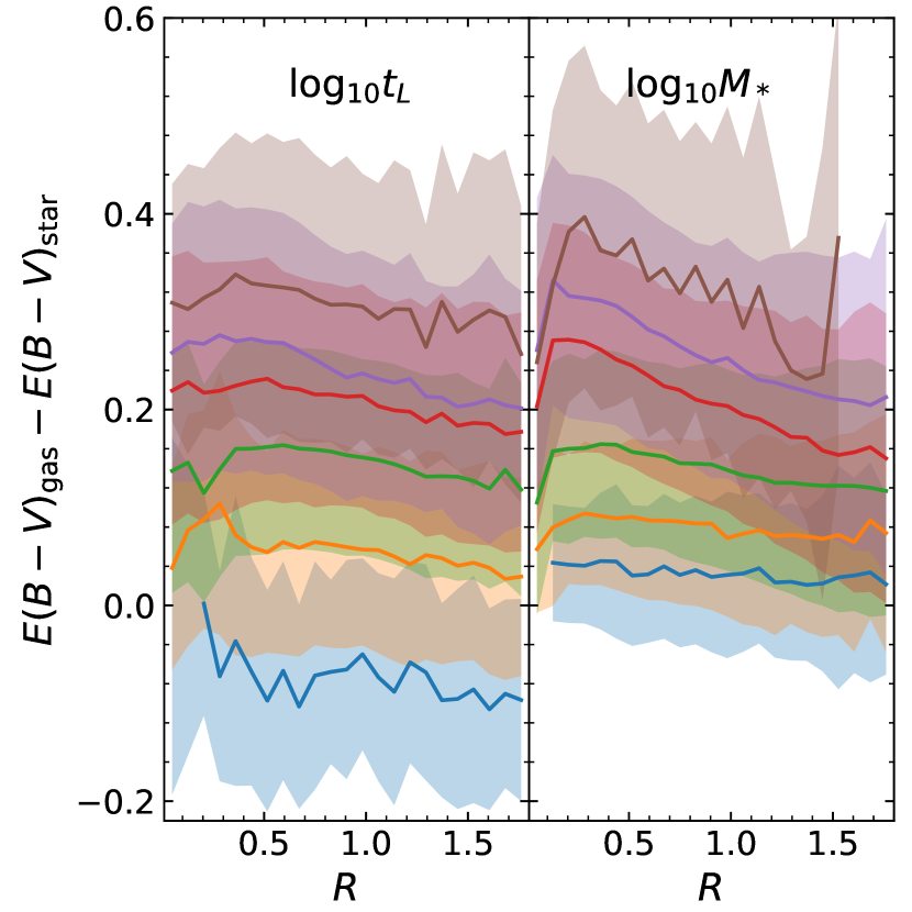
Figure 18: The median radial profiles of the gas-to-stellar attenuation difference for ionized gas regions with different $\log_{10}$$t_{L}$ (left panel) or $\log_{10}$$M_{\ast}$ (right panel). The shaded regions indicate the $1\sigma$ scatter of the regions around the median profile.

4.1.2 Comparison with Greener et al. (2020)

Greener et al. (2020) have recently studied the spatially resolved dust attenuation in 232 spiral galaxies from the eighth MaNGA Product Launch (MPL-8) with morphological classifications from Galaxy Zoo:3D (Masters & Galaxy Zoo Team, 2020). The stellar dust attenuation was measured using the full-spectrum stellar population fitting code STARLIGHT (Cid Fernandes et al., 2005; Cid Fernandes, 2018), with SSPs from the E-MILES (Vazdekis et al., 2010, 2016) templates and a Calzetti et al. (2000) attenuation curve with $R_{V}=4.05$, while the gas dust attenuation was measured from the Balmer decrement assuming $R_{V}=3.1$.

The authors found that dust attenuation increases with $\Sigma_{\rm SFR}$ (SFR surface density), consistent with the positive correlations of both $E(B-V)_{\rm star}$ and $E(B-V)_{\rm gas}$ with $\Sigma_{\rm H\alpha}$ seen from Figure 7, and that the ratio $E(B-V)_{\rm star}/E(B-V)_{\rm gas}$ decreases with $M_{*}$, which is also seen from our data. They found that both $E(B-V)_{\rm star}$ and $E(B-V)_{\rm gas}$ decrease as one goes from the galactic center outwards, which is also seen from our data. They also found that the ratio $E(B-V)_{\rm star}/E(B-V)_{\rm gas}$ has no correlation with the distance from galactic center ($R$), while our data show a weak correlation between $E(B-V)_{\rm star}/E(B-V)_{\rm gas}$ and $R$, with $\rho=0.25$ for all the ionized gas regions and $\rho=0.24$ for Hii regions. In addition, Greener et al. (2020) found a high concentration of birth clouds near the galactic center, as indicated by a negative radial gradient in $E(B-V)_{\rm gas}-E(B-V)_{\rm star}$. As can be seen from Figure 18 (the right panel), our data also show such negative radial profiles at fixed stellar mass and the gradient is stronger at higher mass. We find, however, that the gradient becomes rather weak when the ionized gas regions are limited to narrow ranges of $\log_{10}$$t_{L}$, as shown in the left panel of the same figure. Therefore, the higher $E(B-V)_{\rm gas}$$-$$E(B-V)_{\rm star}$ at smaller $R$ should be attributed to the positive correlation of $E(B-V)_{\rm gas}$$-$$E(B-V)_{\rm star}$ with stellar age (see Figure 7), given that the stellar populations in the inner regions of galaxies are typically older than those in the outer regions. We notice from Figure 18 a weak upturn within $\sim 0.5R_{e}$ in the $E(B-V)_{\rm gas}-E(B-V)_{\rm star}$ of the youngest regions. This may be explained if birth clouds are concentrated in the central regions of galaxies, as suggested by Greener et al. (2020), because very young stars are mostly embedded in birth clouds. However, this result should not be overemphasized, given that the upturn is weak and the noise level is high. We will come back to this in the future.

4.2 Implications of ionizing source for DIG

We find that in DIG regions, $E(B-V)_{\rm star}$ is weakly correlated with $E(B-V)_{\rm gas}$ and in many cases $E(B-V)_{\rm star}$ is larger than $E(B-V)_{\rm gas}$. The behavior is very different from that for Hii regions. Hii regions are mostly located below the 1:1 relation in the $E(B-V)_{\rm star}$ versus $E(B-V)_{\rm gas}$ diagram and follow the $E(B-V)_{\rm star}$$\;=0.44$$E(B-V)_{\rm gas}$ relation on average (Figure 16). For DIG regions, most of the scatter in the relation between $E(B-V)_{\rm star}$ and $E(B-V)_{\rm gas}$ can be explained by the variance in stellar age, as shown in Section 3.4 and Figure 17.

The different behaviors of the dust attenuation between DIG and Hii regions imply that the emission in the two classes are produced by different mechanisms. The physical origin of the DIG is not clear. A variety of ionizing sources have been proposed for the DIG, including supernova shocks, cosmic rays, leaky radiation from Hii regions, and hot evolved stars (e.g., Reynolds & Cox, 1992; Haffner et al., 2009; Yan & Blanton, 2012; Barnes et al., 2014, 2015; Zhang et al., 2017). Using MaNGA data, Zhang et al. (2017) examined the ionization and metallicity diagnostics of DIG-dominated regions, finding that DIG has a lower ionization level than Hii regions, which can enhance $\rm[NII]/H\alpha$, $\rm[SII]/H\alpha$, $\rm[OII]/H\alpha$ and $\rm[OI]/H\alpha$, but reduce $\rm[OIII]/H\beta$. As the leaky Hii region model cannot produce LINER-like emission commonly seen in DIG regions, the authors suggested that hot evolved stars could be a major ionization source for DIG, at least in the following two cases: (1) low-surface brightness regions that are located far from Hii regions, such as regions at large vertical height, and (2) post-starburst galaxies and quiescent galaxies.

Our data support the suggestion of Zhang et al. (2017). In Figure 19 we plot $E(B-V)_{\rm gas}$ as a function of both $b/a$ and $\log_{10}$$t_{L}$, for DIG regions with $\Sigma_{\rm H\alpha}$$\;<10^{38.5}$$\rm erg\;s^{-1}\;kpc^{-2}$. Here we use a $\Sigma_{\rm H\alpha}$ limit 0.5 dex smaller than the usually adopted value to reduce the contamination of the Hii regions. For comparison, the results for the Hii regions with $\Sigma_{\rm H\alpha}$$\;>10^{39}$$\rm erg\;s^{-1}\;kpc^{-2}$ are also plotted, as blue solid/dashed lines. Overall, the DIG and Hii regions behave quite differently, in the sense that $E(B-V)_{\rm gas}$ depends on both $b/a$ and $\log_{10}$$t_{L}$ in Hii regions but $E(B-V)_{\rm gas}$ shows no dependence on either parameter in DIG regions. In addition, the median value of $E(B-V)_{\rm gas}$ in DIG regions is pretty small, constantly at $\sim 0.1$ mag for all values of $b/a$ and $\log_{10}$$t_{L}$. This weak gas attenuation in DIG regions and its independence of $b/a$ strongly indicates that the ionizing source for DIG is distributed in the outskirts of galaxies, either at large vertical heights or at large radial distances, or both. Ionizing photons emerging from these locations can easily escape the galaxy without being attenuated much because of the short propagation path through the ISM, thus leading to $E(B-V)_{\rm gas}$ values that are small and similar in different viewing angles.

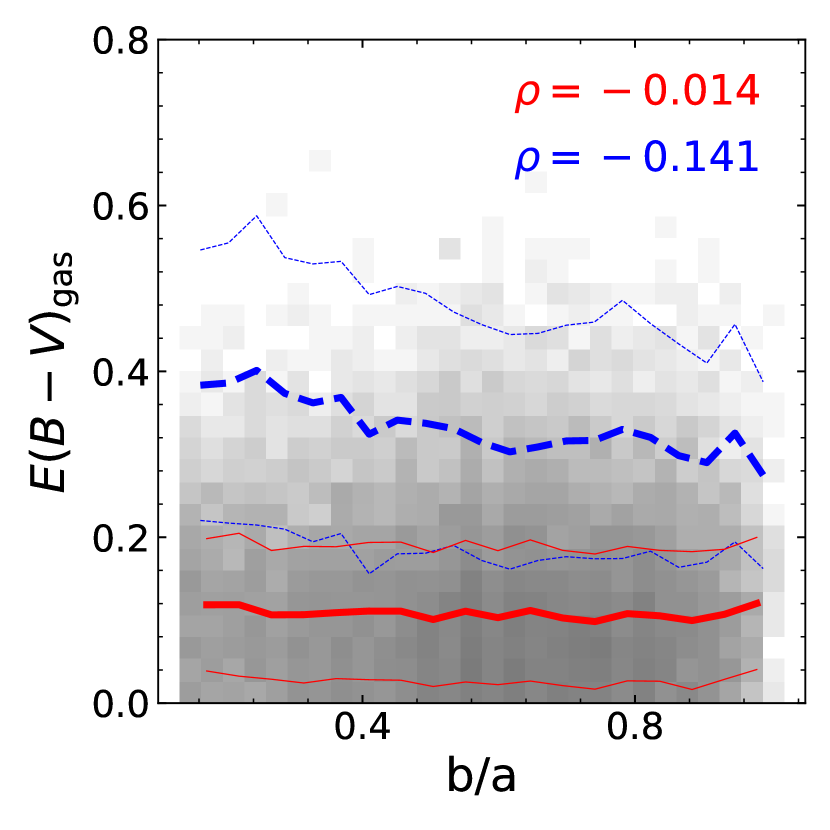
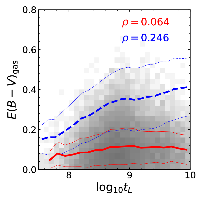
Figure 19: $E(B-V)_{\rm gas}$ as function of $b/a$ (left) and $\log_{10}$$t_{L}$ (right) for DIG regions with $\Sigma_{\rm H\alpha}$$\;<10^{38.5}$$\rm erg\;s^{-1}\;kpc^{-2}$ (red lines) and Hii regions with $\Sigma_{\rm H\alpha}$$\;>10^{39}$$\rm erg\;s^{-1}\;kpc^{-2}$ (blue lines). The number density distribution of the DIG regions is plotted as the gray-scale background. The solid lines are the median relations and the dashed lines indicate the $1\sigma$ scatter of the DIG or Hii regions around the median relation. The Spearman rank correlation coefficients are indicated for both types of regions, with red for DIG and blue for Hii regions.

Figure 20 shows the stellar attenuation parameter $E(B-V)_{\rm star}$ as a function of $b/a$ and $\log_{10}$$t_{L}$ for the DIG and Hii regions. The two types of regions behave similarly, with $E(B-V)_{\rm star}$ decreasing as both $b/a$ and $\log_{10}$$t_{L}$ increase. For DIG regions, the dependence of $E(B-V)_{\rm star}$ on $b/a$ appears to be contradictory to the independence of $E(B-V)_{\rm gas}$ on $b/a$. The stronger stellar attenuation at smaller $b/a$ indicates that the non-ionizing continuum photons emitted from stars must have propagated a longer path than the ionizing photons emerging in the outskirt of the galaxy. The ionized gas regions are selected from the two-dimensional map of $\Sigma_{\rm H\alpha}$, and so they include emission and attenuation along the line of sight. Therefore, the stellar continuum of each DIG region is not emitted from the DIG region itself, but is the integration of the attenuated continuum photons from all stars in the area covered by the region in question, while the ionizing photons are produced in the DIG region. This conjecture is supported by the similar behaviors of DIG and Hii regions in the right-hand panel of Figure 20, which shows again the driving role of the stellar age in the stellar attenuation.

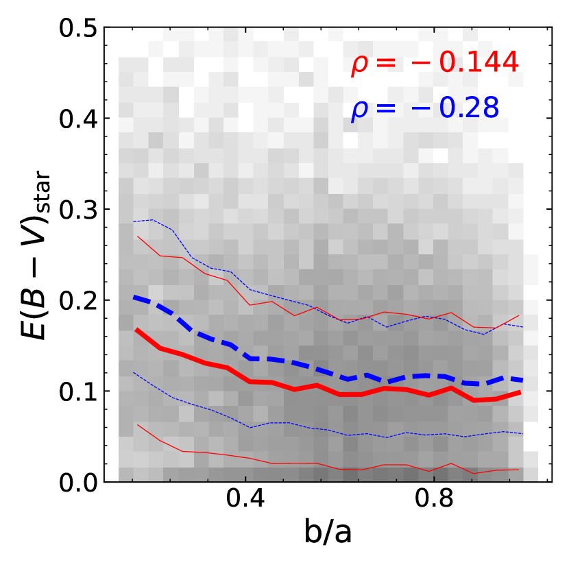
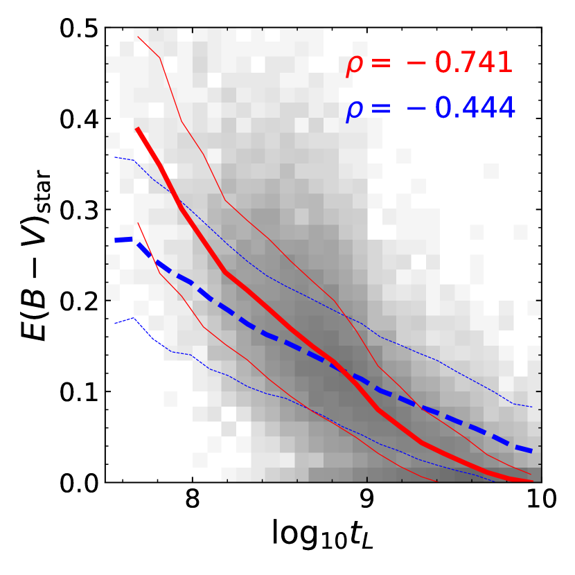
Figure 20: $E(B-V)_{\rm star}$ as function of $b/a$ (left) and $\log_{10}$$t_{L}$ (right) for DIG regions with $\Sigma_{\rm H\alpha}$$\;<10^{38.5}$$\rm erg\;s^{-1}\;kpc^{-2}$ (red lines) and Hii regions with $\Sigma_{\rm H\alpha}$$\;>10^{39}$$\rm erg\;s^{-1}\;kpc^{-2}$ (blue lines). Symbols/lines are the same as in Figure 19.

4.3 The dominant role of stellar age and the dust model of Charlot & Fall (2000)

We find in this paper that the stellar age plays the dominant role in driving the correlation of stellar dust attenuation with many other regional/global properties of galaxies (see Section 3.1). As a result, the stellar age together with $\Sigma_{\rm H\alpha}$ can explain the properties of $E(B-V)_{\rm star}/E(B-V)_{\rm gas}$ in both Hii and DIG regions (see Section 3.4). Among all the correlations considered, the strongest is found between $E(B-V)_{\rm star}/E(B-V)_{\rm gas}$ and $\log_{10}$$t_{L}$  with a Spearman rank correlation coefficient $\rho=-0.63$ (Figure 7). The stellar attenuation itself has a strong correlation also with the stellar age, with $\rho=-0.569$ for the $E(B-V)_{\rm star}$$-$$\log_{10}$$t_{L}$ relation (Figure 7). The negative correlation of $E(B-V)_{\rm star}$ with stellar age is expected, because stars are born in environments with enhanced dust contents (Panuzzo et al., 2007). Such an age-dependent stellar attenuation has been considered in some earlier studies (e.g., Noll et al., 2009; Buat et al., 2012; Lo Faro et al., 2017; Tress et al., 2019).

In DIG regions, the ionizing source is distributed in the outskirts of galaxies while the stellar continuum is dominated by the underlying stars of intermediate/old ages in the ISM (see Section 4.2). Consequently, ionizing photons are less affected by the attenuation than non-ionizing continuum photons. The strong correlation between $E(B-V)_{\rm star}/E(B-V)_{\rm gas}$ and $\log_{10}$$t_{L}$ actually reveals the expected correlation between $E(B-V)_{\rm star}$ and $\log_{10}$$t_{L}$ in DIG regions.

In Hii regions, our results are broadly consistent with the dust model of Charlot & Fall (2000). In this model, non-ionizing continuum photons emitted by young stars and ionizing photons propagate through both the Hi envelope of the “birth clouds”, where young stars are born and embedded, before propagating through the ambient ISM, while emission from long-lived (old) stars only propagate through the ISM because of the finite lifetime of the stellar birth clouds. As emphasized in Charlot & Fall (2000), the finite lifetime of birth clouds is a key ingredient for resolving the discrepancy between the attenuation of line and continuum photons. In very young Hii regions, most of the stars are still embedded in “birth clouds”, so that the stellar attenuation is comparable to the gas attenuation. Basu-Zych et al. (2007) studied a sample of Ultraviolet-luminous galaxies whose $E(B-V)_{\rm star}$ are comparable to $E(B-V)_{\rm gas}$. They found that galaxies whose stars formed only recently are very young and can be explained by a model where the majority of stars are within birth clouds. In very old Hii regions, where the stellar continuum is dominated by old stars in the ISM, both $E(B-V)_{\rm star}$ and $E(B-V)_{\rm star}/E(B-V)_{\rm gas}$ are low, as seen in Figure 7. The intermediate-age Hii regions may be considered as a mixture of both young Hii regions and old Hii regions, so that their $E(B-V)_{\rm star}/E(B-V)_{\rm gas}$ cover the whole range from zero to unity. This is supported by the results shown in Figure 16, where younger Hii regions tend to have steeper slope, and almost all the regions are below the 1:1 relation at $\log_{10}$$\Sigma_{\rm H\alpha}$$\;>39.5$.

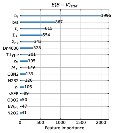
Figure 21: (a)

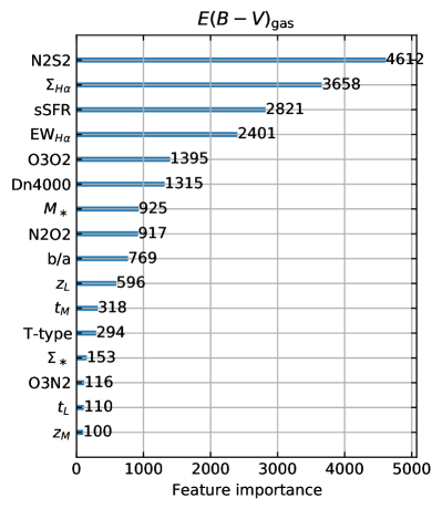
Figure 22: (b)

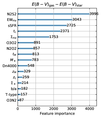
Figure 23: (c)

Figure 24: (d)

Figure 25: Feature importance of the 16 regional/global properties is shown respectively for the four dust attenuation parameters (panels a,b,c,d): $E(B-V)_{\rm star}$, $E(B-V)_{\rm gas}$, $E(B-V)_{\rm gas}-E(B-V)_{\rm star}$, $E(B-V)_{\rm star}/E(B-V)_{\rm gas}$. N2S2, N2O2, O3O2 represent [Nii]/[Sii], [Nii]/[Oii], [Oiii]/[Oii].

4.4 Feature importance of the properties based on machine learning

In Section 3.1 we have examined the correlation of dust attenuations with a large number of regional/global properties. The relative importance of different properties is quantified by the commonly used Spearman rank correlation coefficient. Nowadays, the technique of machine learning has been widely applied to more efficiently deal with such big-data problems. Here we have also done a machine-learning analysis as a consistency check on our results. We use LightGBM , which is a gradient boosting framework using tree-based learning algorithms to evaluate feature importance of the regional/global properties of our galaxies to the dust attenuation parameters.

Figure 25 shows the feature importance of all the 16 properties for $E(B-V)_{\rm star}$, $E(B-V)_{\rm gas}$, $E(B-V)_{\rm gas}-E(B-V)_{\rm star}$ and $E(B-V)_{\rm star}/E(B-V)_{\rm gas}$, respectively. Overall, it is encouraging that the results are well consistent with our previous analysis based on Spearman correlation coefficients: stellar age is indeed the most important property to $E(B-V)_{\rm star}$ and $E(B-V)_{\rm star}/E(B-V)_{\rm gas}$, and [Nii]/[Sii] and $\Sigma_{\rm H\alpha}$ are the most important to $E(B-V)_{\rm gas}$. In particular, the mass-weighted age ($t_{M}$) shows the highest feature importance to $E(B-V)_{\rm star}$, while the luminosity-weighted age ($t_{L}$) is most important to $E(B-V)_{\rm star}/E(B-V)_{\rm gas}$. This is also in good agreement with the Spearman correlation analysis, where $E(B-V)_{\rm star}$ has a correlation coefficient of $\rho=-0.627$ with $t_{M}$ (Figure 26) and $\rho=-0.529$ with $t_{L}$ (Figure 7), and the strongest correlation is found between $E(B-V)_{\rm star}/E(B-V)_{\rm gas}$ and $t_{L}$ with $\rho=-0.631$ (Figure 7). It is interesting to note that the $b/a$ shows a high feature importance to $E(B-V)_{\rm star}$, falling in between $t_{M}$ and $t_{L}$ in panel (a) of the figure. The Spearman correlation coefficient between $E(B-V)_{\rm star}$ and $b/a$ is relatively low ($\rho=-0.228$; Figure 26), however. This is probably because the $b/a$ is a global parameter, thus more sensitive to the overall stellar dust attenuation of the whole galaxy, while the Spearman correlation coefficients simply reflect the average behavior of individual regions. In this regard, the machine learning appears to be more powerful in comprehensively revealing the intrinsic correlations in a complex, high-dimensional dataset.

5 summary

In this paper, we study the relationship between $E(B-V)_{\rm star}$ and $E(B-V)_{\rm gas}$ in both Hii regions and DIG regions of kpc scales, using data of integral field spectroscopy from the MaNGA MPL-9. For each region, we stack the original spectra and perform full spectral fitting to obtain $E(B-V)_{\rm star}$ and other properties of the underlying stellar populations. We then measure emission lines from the starlight-subtracted spectra and calculate $E(B-V)_{\rm gas}$ from the Balmer decrement. With these measurements, we examine the correlations of $E(B-V)_{\rm star}$, $E(B-V)_{\rm gas}$, $E(B-V)_{\rm gas}-E(B-V)_{\rm star}$ and $E(B-V)_{\rm star}/E(B-V)_{\rm gas}$ with 16 regional/global properties. Our main results can be summarized as follows.

• The relation between $E(B-V)_{\rm star}$ and $E(B-V)_{\rm gas}$ is stronger for more active Hii regions.

• Stellar age is the driving factor for $E(B-V)_{\rm star}$, and consequently for $E(B-V)_{\rm gas}-E(B-V)_{\rm star}$ and $E(B-V)_{\rm star}/E(B-V)_{\rm gas}$ as well. At fixed $\Sigma_{\rm H\alpha}$, the stellar age is linearly and negatively correlated with $E(B-V)_{\rm star}/E(B-V)_{\rm gas}$ at all ages.

• Gas-phase metallicity and ionization level are important for $E(B-V)_{\rm gas}$.

• The ionizing sources for DIG regions are likely distributed in the outskirt of galaxies.

• The attenuation in Hii regions can be well explained by the two-component dust model of Charlot & Fall (2000).

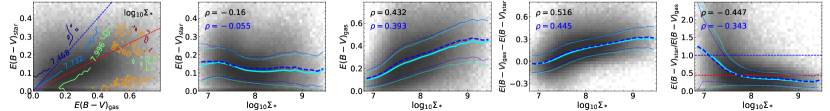
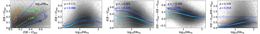
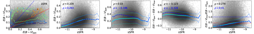
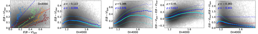
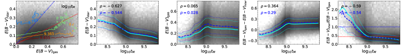
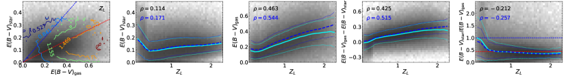
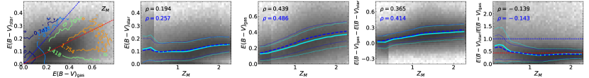
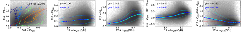
Figure 26: Correlations of $E(B-V)_{\rm star}$ and $E(B-V)_{\rm gas}$ on regional/global properties (panels from top to bottom): $\log_{10}$$\Sigma_{*}$, $\log_{10}$$\rm{EW}_{H\alpha}$, sSFR, $D_{n}4000$, $\log_{10}$$t_{M}$, $Z_{L}$, $Z_{M}$, 12+$\log_{10}$(O/H), $\log_{10}$([Nii]/[Oii]), $\log_{10}$([Oiii]/[Oii]), $\log_{10}$$M_{*}$, $T$-type and $b/a$. Symbols/lines are the same as in Figure 7.

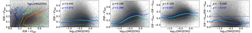
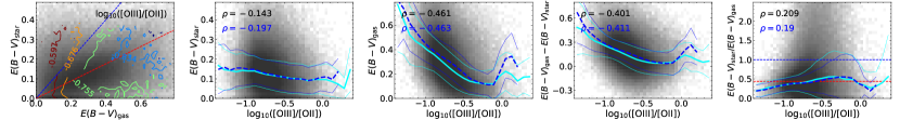
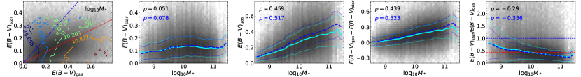
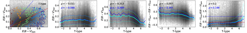
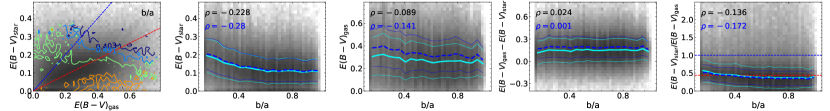
Figure 26: (Continued.)

Appendix A Correlations of dust attenuation parameters with regional/global properties

In the paper we have examined the correlation of dust attenuation with 13 regional properties and 3 global properties. Among other properties, $\log_{10}$$t_{L}$, $\Sigma_{\rm H\alpha}$ and [Nii]/[Sii] are found to be mostly correlated with the dust attenuation parameters, as shown in Figure 7 and discussed in detail in Section 3.1. Here we present the results for the rest 13 properties. Following the format of Figure 7, Figure 26 shows the distribution of each property on the diagram of $E(B-V)_{\rm star}$ versus $E(B-V)_{\rm gas}$, as well as the correlation of the dust attenuation parameters with the properties. The Spearman rank correlation coefficient is indicated in each panel, for both the full sample and the subset of Hii regions as selected by $\log_{10}$$\Sigma_{\rm H\alpha}$$\;>39$. This figure, together with Figure 7, is discussed in depth in the paper. In what follows we briefly mention several interesting points that can be obtained from the figure.

A dichotomy is present in the relation between the attenuation and $\Sigma_{*}$  in the sense that the ionized gas regions can be divided into two classes separated at $\log_{10}$$\Sigma_{\ast}\sim 8$. This can be seen, for instance, from the top-right panel where $E(B-V)_{\rm star}/E(B-V)_{\rm gas}$ decreases rapidly at $\log_{10}$$\Sigma_{\ast}<8$ and levels off at $\sim 0.5$ when $\log_{10}$$\Sigma_{\ast}$ exceeds $\sim 8$, a behavior very similar to the dichotomy in the relation between the attenuations and $\Sigma_{\rm H\alpha}$ as seen in the middle-right panel of Figure 7. This similarity may be understood from the main sequence of star forming regions of galaxies, in which SFR is strongly correlated with stellar mass (e.g., Noeske et al., 2007; Peng et al., 2010; Whitaker et al., 2012; Cano-Díaz et al., 2016; Hsieh et al., 2017).

Our result reveal a positive correlation between $E(B-V)_{\rm star}/E(B-V)_{\rm gas}$ and sSFR, with $\rho=0.274$ (the last panel in the third row). This is consistent with many previous studies based on integrated spectra of galaxies (e.g., Wild et al., 2011; Price et al., 2014; Qin et al., 2019; Koyama et al., 2019), but is different from that of Lin & Kong (2020), who found a negative correlation with $\rho\sim-0.24$. In our case, the attenuation parameters depend on $\rm{EW}_{H\alpha}$ and sSFR in a similar way, which is expected as $\rm{EW}_{H\alpha}$ quantifies the strength of the $\rm H{\alpha}$ luminosity (essentially the SFR) relative to the stellar continuum luminosity (roughly proportional to $\Sigma_{\ast}$). For regions with $\log_{10}$$\rm{EW}_{H\alpha}$$\;\gtrsim 1$ or sSFR$\;\gtrsim-10$, $E(B-V)_{\rm gas}-E(B-V)_{\rm star}$ is roughly constant at around zero and $E(B-V)_{\rm star}/E(B-V)_{\rm gas}$ is close to the value of 0.44, with weak dependence on $\rm{EW}_{H\alpha}$ or sSFR. At lower $\rm{EW}_{H\alpha}$ and sSFR, both attenuation parameters are positively correlated with the two properties, with $E(B-V)_{\rm gas}-E(B-V)_{\rm star}$$\;>0$ and $E(B-V)_{\rm star}/E(B-V)_{\rm gas}$$\;<0.44$.

Overall, all the dust attenuation parameters are weakly correlated with stellar metallicity, except the most metal-poor regions which appear to have higher $E(B-V)_{\rm star}$ and $E(B-V)_{\rm star}/E(B-V)_{\rm gas}$. The age $t_{M}$ shows similar behaviors to $t_{L}$ in its correlations with the attenuation parameters, but the correlation is much weeker for $t_{M}\gtrsim 1$Gyr. The absence of a strong correlation at $t_{M}\gtrsim 1$Gyr is particularly remarkable for $E(B-V)_{\rm gas}$. This result may be understood from the fact that $t_{M}$ is dominated by low-mass old stars which contribute little to dust-related processes. As an empirical indicator of mean stellar age, the 4000Å break is also correlated with the attenuation parameters, as expected. Similar to $t_{M}$, $D_{n}4000$ shows no correlation with $E(B-V)_{\rm gas}$ in old regions with $D_{n}4000\gtrsim 1.5$, which may be explained by the know fact that $D_{n}4000$ is sensitive only to stellar populations younger than 1-2Gyr (e.g., Kauffmann et al., 2003b).

The gas-phase metallicity $12+\log_{10}(\rm O/H)$ is estimated with the O3N2 estimator. The line ratio of [Nii]/[Oii] has also been frequently used to estimate the gas-phase metallicity, particularly when contribution from DIG becomes important (Zhang et al., 2017). Both parameters show weak correlation with $E(B-V)_{\rm star}$, positive correlation with $E(B-V)_{\rm gas}$ and $E(B-V)_{\rm gas}-E(B-V)_{\rm star}$, and negative correlation with $E(B-V)_{\rm star}/E(B-V)_{\rm gas}$. The behaviors of $12+\log_{10}(\rm O/H)$ are quite similar to [Nii]/[Sii], but with weaker correlations with all the dust attenuation parameters. The ionization parameter [Oiii]/[Oii] correlates with all the dust attenuation parameters but in a different way from the metallicity parameters. These trends are broadly consistent with Lin & Kong (2020, see their figure 8).

Figure 26 also shows the correlations of the dust attenuation parameters of ionized gas regions with three global properties of their host galaxies: $M_{*}$, $T$-type and $b/a$. The $E(B-V)_{\rm star}$ shows no obvious correlation with $\log_{10}$$M_{*}$ and $T$-type, but decreases slightly with increasing $b/a$. The latter result is understandable. Smaller $b/a$ correspond to more inclined disks where starlight has to travel through the dusty ISM with a longer path. The $E(B-V)_{\rm gas}$ increases with stellar mass, and shows anti-correlations with $T$-type and $b/a$. The $E(B-V)_{\rm gas}-E(B-V)_{\rm star}$ shows slightly positive correlation with $\log_{10}$$M_{*}$, slightly negative correlation with $T$-type, and weak/no correlation with $b/a$. The $E(B-V)_{\rm star}/E(B-V)_{\rm gas}$ decreases with stellar mass. This result is consistent with that in Lin & Kong (2020), who found that the globally averaged $E(B-V)_{\rm star}/E(B-V)_{\rm gas}$ is a linearly decreasing function of $\log_{10}$$M_{*}$ (see their figure 10). The $E(B-V)_{\rm star}/E(B-V)_{\rm gas}$ shows slightly positive correlation with $T$-type and almost no correlation with $b/a$. Generally, the trends of the dust attenuation parameters with the global properties are consistent with the correlations with the regional properties as described above.

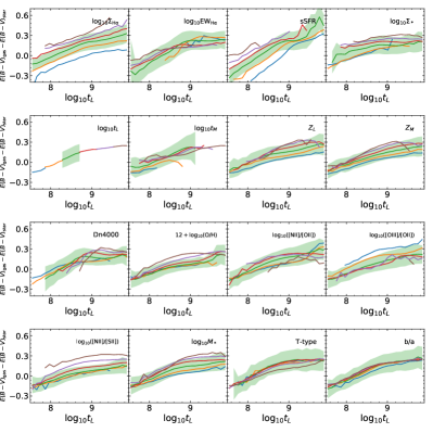
Figure 27: (a) $E(B-V)_{\rm gas}$$-$$E(B-V)_{\rm star}$ versus $\log_{10}$$t_{L}$

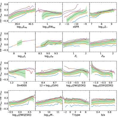
Figure 28: (b) $E(B-V)_{\rm gas}$$-$$E(B-V)_{\rm star}$ versus regional/global properties

Figure 29: $E(B-V)_{\rm gas}$$-$$E(B-V)_{\rm star}$ as function of stellar age ($\log_{10}$$t_{L}$) for ionized gas regions in different intervals of regional/global properties (panels a), and as functions of regional/global properties but in different intervals of $\log_{10}$$t_{L}$ (panels b). Symbols/lines are the same as in Figure 10.

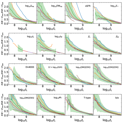
Figure 30: (a) $E(B-V)_{\rm star}/E(B-V)_{\rm gas}$ versus $\log_{10}$$t_{L}$

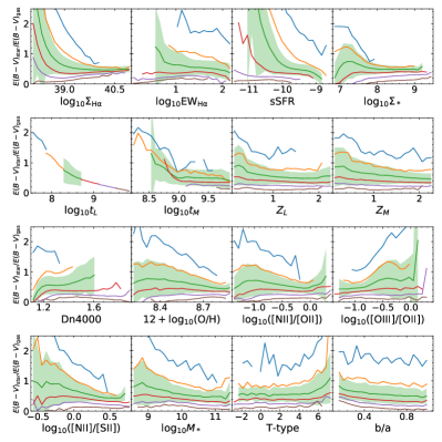
Figure 31: (b) $E(B-V)_{\rm star}/E(B-V)_{\rm gas}$ versus regional/global properties

Figure 32: $E(B-V)_{\rm star}$/$E(B-V)_{\rm gas}$ as functions of stellar age ($\log_{10}$$t_{L}$) but in different intervals of regional/global properties (panels a), and as function of regional/global properties but in different intervals of $\log_{10}$$t_{L}$ (panels b). Symbols/lines are the same as in Figure 10.

Appendix B Role of specific properties in driving dust attenuation

Section 3.2 examines the role of stellar age in driving stellar attenuation, and Section 3.3 investigates the role of $\Sigma_{\rm H\alpha}$, [Nii]/[Sii] and [Oiii]/[Oii] in driving the attenuation in gas. In those sections, for simplicity, results are shown only for some of the dust attenuation parameters or regional/global properties. Here we present the remaining results for completeness.

Figure 29 and Figure 32 show the correlations of the two dust attenuation parameters, $E(B-V)_{\rm gas}-E(B-V)_{\rm star}$ and $E(B-V)_{\rm star}/E(B-V)_{\rm gas}$ respectively, with all the regional/global properties, aiming to test the dominant role of $\log_{10}$$t_{L}$. These figures follow the same format as Figure 10, and provide complementary results to the analysis in Section 3.2. Each figure contains two sets of panels. In panel set (a), the dust attenuation parameter is plotted as function of $\log_{10}$$t_{L}$, but for different subsets of the ionized gas regions selected by different regional/global properties. In panel set (b), the full sample is divided into subsets according to $\log_{10}$$t_{L}$, and the dust attenuation parameter of each subset is plotted as function of the different regional/global properties. Figure 10 shows that stellar age is indeed a driving property for the stellar attenuation. The two figures here further show that the stellar age also plays an important role in driving the difference and ratio between the stellar and gas attenuation. This result is produced by the combined effect of the strong correlation of $\log_{10}$$t_{L}$ with $E(B-V)_{\rm star}$ and the moderate correlation of $\log_{10}$$t_{L}$ with $E(B-V)_{\rm gas}$, as discussed in Sections 3.2 and 3.3.

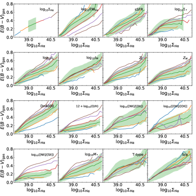
Figure 33: (a) $E(B-V)_{\rm gas}$ versus $\log_{10}$$\Sigma_{\rm H\alpha}$

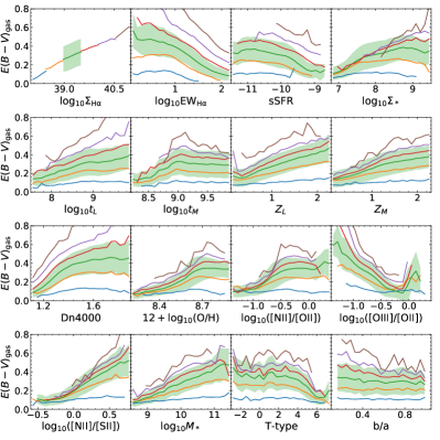
Figure 34: (b) $E(B-V)_{\rm gas}$ versus regional/global properties

Figure 35: $E(B-V)_{\rm gas}$ as functions of $\Sigma_{\rm H\alpha}$ but in different intervals of regional/global properties (panels a), and as function of regional/global properties but in different intervals of $\Sigma_{\rm H\alpha}$ (panels b). Symbols/lines are the same as in Figure 10.

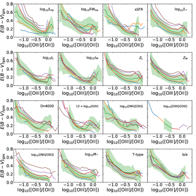
Figure 36: (a) $E(B-V)_{\rm gas}$ versus $\log_{10}$[Oiii]/[Oii]

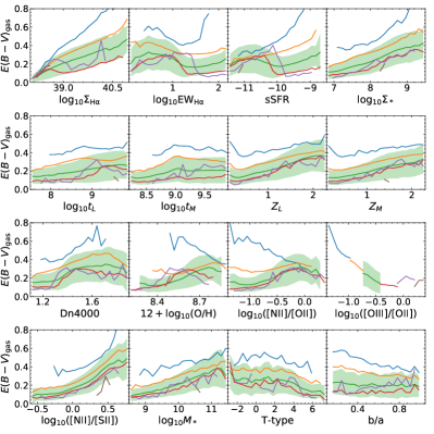
Figure 37: (b) $E(B-V)_{\rm gas}$ versus regional/global properties

Figure 38: $E(B-V)_{\rm gas}$ as functions of [Oiii]/[Oii] but in different intervals of regional/global properties (panels a), and as function of regional/global properties but in different intervals of [Oiii]/[Oii] (panels b). Symbols/lines are the same as in Figure 10.

Figure 35 and Figure 38 examine the correlation of $E(B-V)_{\rm gas}$ with the 16 regional/global properties, aiming to test the importance of $\Sigma_{\rm H\alpha}$ and [Oiii]/[Oii] in driving the attenuation in gas. These figures follow the same format as Figure 13 which tests the role of [Nii]/[Sii], and provide complementary results to the analysis in Section 3.3. Each figure contains two sets of panels, with one plotting $E(B-V)_{\rm gas}$ as a function of either $\Sigma_{\rm H\alpha}$ or [Oiii]/[Oii] for subsets of ionized gas regions selected by different properties, and the other plotting $E(B-V)_{\rm gas}$ as a function of different properties for subsets of ionized gas regions selected by either $\Sigma_{\rm H\alpha}$ or [Oiii]/[Oii]. Comparing the two figures here with Figure 13, one can find that [Nii]/[Sii] shows stronger correlation with the gas attenuation than $\Sigma_{\rm H\alpha}$ and [Oiii]/[Oii].

References

- Aguado et al. (2019) Aguado, D. S., Ahumada, R., Almeida, A., et al. 2019, ApJS, 240, 23, doi: 10.3847/1538-4365/aaf651
- Alloin et al. (1979) Alloin, D., Collin-Souffrin, S., Joly, M., & Vigroux, L. 1979, A&A, 78, 200
- Anderson et al. (2019) Anderson, L. D., Wenger, T. V., Armentrout, W. P., Balser, D. S., & Bania, T. M. 2019, ApJ, 871, 145, doi: 10.3847/1538-4357/aaf571
- Aoyama et al. (2017) Aoyama, S., Hou, K.-C., Shimizu, I., et al. 2017, MNRAS, 466, 105, doi: 10.1093/mnras/stw3061
- Asari et al. (2007) Asari, N. V., Cid Fernandes, R., Stasińska, G., et al. 2007, MNRAS, 381, 263, doi: 10.1111/j.1365-2966.2007.12255.x
- Baldwin et al. (1981) Baldwin, J. A., Phillips, M. M., & Terlevich, R. 1981, PASP, 93, 5, doi: 10.1086/130766
- Balogh et al. (1999) Balogh, M. L., Morris, S. L., Yee, H. K. C., Carlberg, R. G., & Ellingson, E. 1999, ApJ, 527, 54, doi: 10.1086/308056
- Barnes et al. (2014) Barnes, J. E., Wood, K., Hill, A. S., & Haffner, L. M. 2014, MNRAS, 440, 3027, doi: 10.1093/mnras/stu521
- Barnes et al. (2015) —. 2015, MNRAS, 447, 559, doi: 10.1093/mnras/stu2454
- Basu-Zych et al. (2007) Basu-Zych, A. R., Schiminovich, D., Johnson, B. D., et al. 2007, ApJS, 173, 457, doi: 10.1086/521146
- Battisti et al. (2017a) Battisti, A. J., Calzetti, D., & Chary, R.-R. 2017a, ApJ, 840, 109, doi: 10.3847/1538-4357/aa6fb2
- Battisti et al. (2017b) —. 2017b, ApJ, 851, 90, doi: 10.3847/1538-4357/aa9a43
- Bertelli et al. (1994) Bertelli, G., Bressan, A., Chiosi, C., Fagotto, F., & Nasi, E. 1994, A&AS, 106, 275
- Bianchi & Ferrara (2005) Bianchi, S., & Ferrara, A. 2005, MNRAS, 358, 379, doi: 10.1111/j.1365-2966.2005.08762.x
- Blanton et al. (2011) Blanton, M. R., Kazin, E., Muna, D., Weaver, B. A., & Price-Whelan, A. 2011, AJ, 142, 31, doi: 10.1088/0004-6256/142/1/31
- Blanton et al. (2005) Blanton, M. R., Schlegel, D. J., Strauss, M. A., et al. 2005, AJ, 129, 2562, doi: 10.1086/429803
- Blanton et al. (2017) Blanton, M. R., Bershady, M. A., Abolfathi, B., et al. 2017, AJ, 154, 28, doi: 10.3847/1538-3881/aa7567
- Blitz & Shu (1980) Blitz, L., & Shu, F. H. 1980, ApJ, 238, 148, doi: 10.1086/157968
- Boquien et al. (2019) Boquien, M., Burgarella, D., Roehlly, Y., et al. 2019, A&A, 622, A103, doi: 10.1051/0004-6361/201834156
- Bruzual & Charlot (2003) Bruzual, G., & Charlot, S. 2003, MNRAS, 344, 1000, doi: 10.1046/j.1365-8711.2003.06897.x
- Buat et al. (2018) Buat, V., Boquien, M., Małek, K., et al. 2018, A&A, 619, A135, doi: 10.1051/0004-6361/201833841
- Buat et al. (2012) Buat, V., Noll, S., Burgarella, D., et al. 2012, A&A, 545, A141, doi: 10.1051/0004-6361/201219405
- Bundy et al. (2015) Bundy, K., Bershady, M. A., Law, D. R., et al. 2015, ApJ, 798, 7, doi: 10.1088/0004-637X/798/1/7
- Calzetti et al. (2000) Calzetti, D., Armus, L., Bohlin, R. C., et al. 2000, ApJ, 533, 682, doi: 10.1086/308692
- Calzetti et al. (1994) Calzetti, D., Kinney, A. L., & Storchi-Bergmann, T. 1994, ApJ, 429, 582, doi: 10.1086/174346
- Cano-Díaz et al. (2016) Cano-Díaz, M., Sánchez, S. F., Zibetti, S., et al. 2016, ApJ, 821, L26, doi: 10.3847/2041-8205/821/2/L26
- Cardelli et al. (1989) Cardelli, J. A., Clayton, G. C., & Mathis, J. S. 1989, ApJ, 345, 245, doi: 10.1086/167900
- Chabrier (2003) Chabrier, G. 2003, PASP, 115, 763, doi: 10.1086/376392
- Charlot & Fall (2000) Charlot, S., & Fall, S. M. 2000, ApJ, 539, 718, doi: 10.1086/309250
- Chevallard et al. (2013) Chevallard, J., Charlot, S., Wandelt, B., & Wild, V. 2013, MNRAS, 432, 2061, doi: 10.1093/mnras/stt523
- Cid Fernandes (2018) Cid Fernandes, R. 2018, MNRAS, 480, 4480, doi: 10.1093/mnras/sty2012
- Cid Fernandes et al. (2005) Cid Fernandes, R., Mateus, A., Sodré, L., Stasińska, G., & Gomes, J. M. 2005, MNRAS, 358, 363, doi: 10.1111/j.1365-2966.2005.08752.x
- Cid Fernandes et al. (2013) Cid Fernandes, R., Pérez, E., García Benito, R., et al. 2013, A&A, 557, A86, doi: 10.1051/0004-6361/201220616
- Conroy (2013) Conroy, C. 2013, ARA&A, 51, 393, doi: 10.1146/annurev-astro-082812-141017
- Croom et al. (2012) Croom, S. M., Lawrence, J. S., Bland-Hawthorn, J., et al. 2012, MNRAS, 421, 872, doi: 10.1111/j.1365-2966.2011.20365.x
- Denicoló et al. (2002) Denicoló, G., Terlevich, R., & Terlevich, E. 2002, MNRAS, 330, 69, doi: 10.1046/j.1365-8711.2002.05041.x
- Domínguez Sánchez et al. (2018) Domínguez Sánchez, H., Huertas-Company, M., Bernardi, M., Tuccillo, D., & Fischer, J. L. 2018, MNRAS, 476, 3661, doi: 10.1093/mnras/sty338
- Dominik & Tielens (1997) Dominik, C., & Tielens, A. G. G. M. 1997, ApJ, 480, 647, doi: 10.1086/303996
- Dopita et al. (2013) Dopita, M. A., Sutherland, R. S., Nicholls, D. C., Kewley, L. J., & Vogt, F. P. A. 2013, ApJS, 208, 10, doi: 10.1088/0067-0049/208/1/10
- Drory et al. (2015) Drory, N., MacDonald, N., Bershady, M. A., et al. 2015, AJ, 149, 77, doi: 10.1088/0004-6256/149/2/77
- Dwek (1998) Dwek, E. 1998, ApJ, 501, 643, doi: 10.1086/305829
- Fanelli et al. (1988) Fanelli, M. N., O’Connell, R. W., & Thuan, T. X. 1988, ApJ, 334, 665, doi: 10.1086/166869
- Fitzpatrick (1999) Fitzpatrick, E. L. 1999, PASP, 111, 63, doi: 10.1086/316293
- Galliano et al. (2018) Galliano, F., Galametz, M., & Jones, A. P. 2018, ARA&A, 56, 673, doi: 10.1146/annurev-astro-081817-051900
- Ge et al. (2018) Ge, J., Yan, R., Cappellari, M., et al. 2018, MNRAS, 478, 2633, doi: 10.1093/mnras/sty1245
- González Delgado et al. (2005) González Delgado, R. M., Cerviño, M., Martins, L. P., Leitherer, C., & Hauschildt, P. H. 2005, MNRAS, 357, 945, doi: 10.1111/j.1365-2966.2005.08692.x
- Gordon et al. (2003) Gordon, K. D., Clayton, G. C., Misselt, K. A., Landolt, A. U., & Wolff, M. J. 2003, ApJ, 594, 279, doi: 10.1086/376774
- Gordon et al. (2000) Gordon, K. D., Clayton, G. C., Witt, A. N., & Misselt, K. A. 2000, ApJ, 533, 236, doi: 10.1086/308668
- Greener et al. (2020) Greener, M. J., Aragón-Salamanca, A., Merrifield, M. R., et al. 2020, MNRAS, 495, 2305, doi: 10.1093/mnras/staa1300
- Gunn et al. (2006) Gunn, J. E., Siegmund, W. A., Mannery, E. J., et al. 2006, AJ, 131, 2332, doi: 10.1086/500975
- Haffner et al. (2009) Haffner, L. M., Dettmar, R. J., Beckman, J. E., et al. 2009, Reviews of Modern Physics, 81, 969, doi: 10.1103/RevModPhys.81.969
- Hirashita & Kuo (2011) Hirashita, H., & Kuo, T.-M. 2011, MNRAS, 416, 1340, doi: 10.1111/j.1365-2966.2011.19131.x
- Hsieh et al. (2017) Hsieh, B. C., Lin, L., Lin, J. H., et al. 2017, ApJ, 851, L24, doi: 10.3847/2041-8213/aa9d80
- Hunt & Hirashita (2009) Hunt, L. K., & Hirashita, H. 2009, A&A, 507, 1327, doi: 10.1051/0004-6361/200912020
- Kashino et al. (2013) Kashino, D., Silverman, J. D., Rodighiero, G., et al. 2013, ApJ, 777, L8, doi: 10.1088/2041-8205/777/1/L8
- Kauffmann et al. (2003a) Kauffmann, G., Heckman, T. M., Tremonti, C., et al. 2003a, MNRAS, 346, 1055, doi: 10.1111/j.1365-2966.2003.07154.x
- Kauffmann et al. (2003b) Kauffmann, G., Heckman, T. M., White, S. D. M., et al. 2003b, MNRAS, 341, 33, doi: 10.1046/j.1365-8711.2003.06291.x
- Kennicutt (1984) Kennicutt, R. C., J. 1984, ApJ, 287, 116, doi: 10.1086/162669
- Kennicutt (1998) Kennicutt, Robert C., J. 1998, ARA&A, 36, 189, doi: 10.1146/annurev.astro.36.1.189
- Kewley et al. (2006) Kewley, L. J., Groves, B., Kauffmann, G., & Heckman, T. 2006, MNRAS, 372, 961, doi: 10.1111/j.1365-2966.2006.10859.x
- Kewley et al. (2001) Kewley, L. J., Heisler, C. A., Dopita, M. A., & Lumsden, S. 2001, ApJS, 132, 37, doi: 10.1086/318944
- Kim & Koo (2001) Kim, K.-T., & Koo, B.-C. 2001, ApJ, 549, 979, doi: 10.1086/319447
- Koyama et al. (2019) Koyama, Y., Shimakawa, R., Yamamura, I., Kodama, T., & Hayashi, M. 2019, PASJ, 71, 8, doi: 10.1093/pasj/psy113
- Kreckel et al. (2013) Kreckel, K., Groves, B., Schinnerer, E., et al. 2013, ApJ, 771, 62, doi: 10.1088/0004-637X/771/1/62
- Lacerda et al. (2018) Lacerda, E. A. D., Cid Fernandes, R., Couto, G. S., et al. 2018, MNRAS, 474, 3727, doi: 10.1093/mnras/stx3022
- Law et al. (2016) Law, D. R., Cherinka, B., Yan, R., et al. 2016, AJ, 152, 83, doi: 10.3847/0004-6256/152/4/83
- Li et al. (2005) Li, C., Wang, T.-G., Zhou, H.-Y., Dong, X.-B., & Cheng, F.-Z. 2005, AJ, 129, 669, doi: 10.1086/426909
- Li et al. (2020) Li, N., Li, C., Mo, H., et al. 2020, ApJ, 896, 38, doi: 10.3847/1538-4357/ab92a1
- Liang et al. (2020) Liang, F.-H., Li, C., Li, N., et al. 2020, ApJ, 896, 121, doi: 10.3847/1538-4357/ab9596
- Lin & Kong (2020) Lin, Z., & Kong, X. 2020, ApJ, 888, 88, doi: 10.3847/1538-4357/ab5f0e
- Lo Faro et al. (2017) Lo Faro, B., Buat, V., Roehlly, Y., et al. 2017, MNRAS, 472, 1372, doi: 10.1093/mnras/stx1901
- Lopez et al. (2011) Lopez, L. A., Krumholz, M. R., Bolatto, A. D., Prochaska, J. X., & Ramirez-Ruiz, E. 2011, ApJ, 731, 91, doi: 10.1088/0004-637X/731/2/91
- Masters & Galaxy Zoo Team (2020) Masters, K. L., & Galaxy Zoo Team. 2020, in IAU Symposium, Vol. 353, Galactic Dynamics in the Era of Large Surveys, ed. M. Valluri & J. A. Sellwood, 205–212, doi: 10.1017/S1743921319008615
- Meurer et al. (1999) Meurer, G. R., Heckman, T. M., & Calzetti, D. 1999, ApJ, 521, 64, doi: 10.1086/307523
- Nanni et al. (2013) Nanni, A., Bressan, A., Marigo, P., & Girardi, L. 2013, MNRAS, 434, 2390, doi: 10.1093/mnras/stt1175
- Noeske et al. (2007) Noeske, K. G., Weiner, B. J., Faber, S. M., et al. 2007, ApJ, 660, L43, doi: 10.1086/517926
- Noll et al. (2009) Noll, S., Burgarella, D., Giovannoli, E., et al. 2009, A&A, 507, 1793, doi: 10.1051/0004-6361/200912497
- Nozawa et al. (2007) Nozawa, T., Kozasa, T., Habe, A., et al. 2007, ApJ, 666, 955, doi: 10.1086/520621
- Osterbrock & Ferland (2006) Osterbrock, D. E., & Ferland, G. J. 2006, Astrophysics of gaseous nebulae and active galactic nuclei, 2nd edn. (Sausalito, CA: University Science Books)
- Pannella et al. (2015) Pannella, M., Elbaz, D., Daddi, E., et al. 2015, ApJ, 807, 141, doi: 10.1088/0004-637X/807/2/141
- Panuzzo et al. (2007) Panuzzo, P., Granato, G. L., Buat, V., et al. 2007, MNRAS, 375, 640, doi: 10.1111/j.1365-2966.2006.11337.x
- Peng et al. (2010) Peng, Y.-j., Lilly, S. J., Kovač, K., et al. 2010, ApJ, 721, 193, doi: 10.1088/0004-637X/721/1/193
- Pettini & Pagel (2004) Pettini, M., & Pagel, B. E. J. 2004, MNRAS, 348, L59, doi: 10.1111/j.1365-2966.2004.07591.x
- Pilyugin (2001) Pilyugin, L. S. 2001, A&A, 369, 594, doi: 10.1051/0004-6361:20010079
- Pilyugin & Thuan (2005) Pilyugin, L. S., & Thuan, T. X. 2005, ApJ, 631, 231, doi: 10.1086/432408
- Popping et al. (2017) Popping, G., Somerville, R. S., & Galametz, M. 2017, MNRAS, 471, 3152, doi: 10.1093/mnras/stx1545
- Prevot et al. (1984) Prevot, M. L., Lequeux, J., Maurice, E., Prevot, L., & Rocca-Volmerange, B. 1984, A&A, 132, 389
- Price et al. (2014) Price, S. H., Kriek, M., Brammer, G. B., et al. 2014, ApJ, 788, 86, doi: 10.1088/0004-637X/788/1/86
- Puglisi et al. (2016) Puglisi, A., Rodighiero, G., Franceschini, A., et al. 2016, A&A, 586, A83, doi: 10.1051/0004-6361/201526782
- Qin et al. (2019) Qin, J., Zheng, X. Z., Wuyts, S., Pan, Z., & Ren, J. 2019, ApJ, 886, 28, doi: 10.3847/1538-4357/ab4a04
- Reddy et al. (2010) Reddy, N. A., Erb, D. K., Pettini, M., Steidel, C. C., & Shapley, A. E. 2010, ApJ, 712, 1070, doi: 10.1088/0004-637X/712/2/1070
- Reddy et al. (2015) Reddy, N. A., Kriek, M., Shapley, A. E., et al. 2015, ApJ, 806, 259, doi: 10.1088/0004-637X/806/2/259
- Reynolds & Cox (1992) Reynolds, R. J., & Cox, D. P. 1992, ApJ, 400, L33, doi: 10.1086/186642
- Riffel et al. (2009) Riffel, R., Pastoriza, M. G., Rodríguez-Ardila, A., & Bonatto, C. 2009, MNRAS, 400, 273, doi: 10.1111/j.1365-2966.2009.15448.x
- Riffel et al. (2008) Riffel, R., Pastoriza, M. G., Rodríguez-Ardila, A., & Maraston, C. 2008, MNRAS, 388, 803, doi: 10.1111/j.1365-2966.2008.13440.x
- Riffel et al. (2021) Riffel, R., Mallmann, N. D., Ilha, G. S., et al. 2021, MNRAS, 501, 4064, doi: 10.1093/mnras/staa3907
- Salim & Narayanan (2020) Salim, S., & Narayanan, D. 2020, ARA&A, 58, 529, doi: 10.1146/annurev-astro-032620-021933
- Sánchez et al. (2012a) Sánchez, S. F., Kennicutt, R. C., Gil de Paz, A., et al. 2012a, A&A, 538, A8, doi: 10.1051/0004-6361/201117353
- Sánchez et al. (2012b) Sánchez, S. F., Rosales-Ortega, F. F., Marino, R. A., et al. 2012b, A&A, 546, A2, doi: 10.1051/0004-6361/201219578
- Sánchez et al. (2018) Sánchez, S. F., Avila-Reese, V., Hernandez-Toledo, H., et al. 2018, Rev. Mexicana Astron. Astrofis., 54, 217. https://arxiv.org/abs/1709.05438
- Schneider et al. (2014) Schneider, R., Valiante, R., Ventura, P., et al. 2014, MNRAS, 442, 1440, doi: 10.1093/mnras/stu861
- Smee et al. (2013) Smee, S. A., Gunn, J. E., Uomoto, A., et al. 2013, AJ, 146, 32, doi: 10.1088/0004-6256/146/2/32
- Tomičić et al. (2017) Tomičić, N., Kreckel, K., Groves, B., et al. 2017, ApJ, 844, 155, doi: 10.3847/1538-4357/aa7b30
- Tremonti et al. (2004) Tremonti, C. A., Heckman, T. M., Kauffmann, G., et al. 2004, ApJ, 613, 898, doi: 10.1086/423264
- Tress et al. (2019) Tress, M., Ferreras, I., Pérez-González, P. G., et al. 2019, MNRAS, 488, 2301, doi: 10.1093/mnras/stz1851
- Urrutia et al. (2019) Urrutia, T., Wisotzki, L., Kerutt, J., et al. 2019, A&A, 624, A141, doi: 10.1051/0004-6361/201834656
- Valentino et al. (2015) Valentino, F., Daddi, E., Strazzullo, V., et al. 2015, ApJ, 801, 132, doi: 10.1088/0004-637X/801/2/132
- Vazdekis et al. (2016) Vazdekis, A., Koleva, M., Ricciardelli, E., Röck, B., & Falcón-Barroso, J. 2016, MNRAS, 463, 3409, doi: 10.1093/mnras/stw2231
- Vazdekis et al. (2010) Vazdekis, A., Sánchez-Blázquez, P., Falcón-Barroso, J., et al. 2010, MNRAS, 404, 1639, doi: 10.1111/j.1365-2966.2010.16407.x
- Wake et al. (2017) Wake, D. A., Bundy, K., Diamond-Stanic, A. M., et al. 2017, AJ, 154, 86, doi: 10.3847/1538-3881/aa7ecc
- Westfall et al. (2019) Westfall, K. B., Cappellari, M., Bershady, M. A., et al. 2019, AJ, 158, 231, doi: 10.3847/1538-3881/ab44a2
- Whitaker et al. (2012) Whitaker, K. E., van Dokkum, P. G., Brammer, G., & Franx, M. 2012, ApJ, 754, L29, doi: 10.1088/2041-8205/754/2/L29
- Wild et al. (2011) Wild, V., Charlot, S., Brinchmann, J., et al. 2011, MNRAS, 417, 1760, doi: 10.1111/j.1365-2966.2011.19367.x
- Wilkinson et al. (2015) Wilkinson, D. M., Maraston, C., Thomas, D., et al. 2015, MNRAS, 449, 328, doi: 10.1093/mnras/stv301
- Wuyts et al. (2011) Wuyts, S., Förster Schreiber, N. M., Lutz, D., et al. 2011, ApJ, 738, 106, doi: 10.1088/0004-637X/738/1/106
- Wuyts et al. (2013) Wuyts, S., Förster Schreiber, N. M., Nelson, E. J., et al. 2013, ApJ, 779, 135, doi: 10.1088/0004-637X/779/2/135
- Yan & Blanton (2012) Yan, R., & Blanton, M. R. 2012, ApJ, 747, 61, doi: 10.1088/0004-637X/747/1/61
- Yan et al. (2016a) Yan, R., Tremonti, C., Bershady, M. A., et al. 2016a, AJ, 151, 8, doi: 10.3847/0004-6256/151/1/8
- Yan et al. (2016b) Yan, R., Bundy, K., Law, D. R., et al. 2016b, AJ, 152, 197, doi: 10.3847/0004-6256/152/6/197
- Zahid et al. (2017) Zahid, H. J., Kudritzki, R.-P., Conroy, C., Andrews, B., & Ho, I. T. 2017, ApJ, 847, 18, doi: 10.3847/1538-4357/aa88ae
- Zaritsky et al. (1994) Zaritsky, D., Kennicutt, Robert C., J., & Huchra, J. P. 1994, ApJ, 420, 87, doi: 10.1086/173544
- Zhang et al. (2017) Zhang, K., Yan, R., Bundy, K., et al. 2017, MNRAS, 466, 3217, doi: 10.1093/mnras/stw3308
- Zhou et al. (2019) Zhou, S., Mo, H. J., Li, C., et al. 2019, MNRAS, 485, 5256, doi: 10.1093/mnras/stz764
- Zhukovska (2014) Zhukovska, S. 2014, A&A, 562, A76, doi: 10.1051/0004-6361/201322989