Antipredator behavior in the rock-paper-scissors model

Abstract

When faced with an imminent risk of predation, many animals react to escape consumption. Antipredator strategies are performed by individuals acting as a group to intimidate predators and minimize the damage when attacked. We study the antipredator prey response in spatial tritrophic systems with cyclic species dominance using the rock-paper-scissors game. The impact of the antipredator behavior is local, with the predation probability reducing exponentially with the number of preys in the predator’s neighborhood. In contrast to the standard Lotka-Volterra implementation of the rock-paper-scissors model, where no spiral waves appear, our outcomes show that the antipredator behavior leads to spiral patterns from random initial conditions. The results show that the predation risk decreases exponentially with the level of antipredator strength. Finally, we investigate the coexistence probability and verify that antipredator behavior may jeopardize biodiversity for high mobility. Our findings may help biologists to understand ecosystems formed by species whose individuals behave strategically to resist predation.

I Introduction

The spatial segregation of species is a fundamental issue in ecologyBegon et al. (2006). To this purpose, many authors have conducted experimental and theoretical studies to understand how interactions among individuals are responsible for ecosystem formation and stability Purvis and Hector (2000); Buchholz (2007). In this scenario, the experiments with bacteria Escherichia coli unveiled the role of space to preserve biodiversity Kerr et al. (2002). There is a cyclic dominance among three bacteria strains that can be described by the rock-paper-scissors game rules Kirkup and Riley (2004). However, the cyclic dominance is not sufficient to guarantee coexistence, but individuals must interact locally. The consequence is the formation of spatial domains occupied mostly by individuals of the same species Durret and Levin (1997). The same phenomenon is observed in groups of lizards Sinervo and Lively (1996) and coral reefs Volkov et al. (2007).

Given the relevance of the cyclic dominance in maintaining biodiversity, stochastic simulations of the rock-paper-scissors model have been an essential tool to comprehend how spatial patterns appear and affect species persistence Szolnoki et al. (2020, 2014). The simulations may be realized either considering a conservation law for the total number of individuals (Lotka-Volterra implementation Lotka (1920); Volterra ((1931)) or with the presence of a variable density of empty spaces (May-Leonard implementation Reichenbach et al. (2007); Avelino et al. (2012); Menezes et al. (2019)). This paper focuses on the Lotka-Volterra version, where random mobility competes with local predation interaction. In this case, the spiral patterns observed in the May-Leonard stochastic simulations of the rock-paper-scissors models are not present, as shown in Ref. Peltomäki and Alava (2008) (see also Cheng et al. (2018); Avelino et al. (2014); Pereira et al. (2018); Avelino et al. (2019) for generalizations of the rock-paper-scissors game).

It is well known that behavioral strategies play a vital role in evolutionary biology Buchholz (2007). For example, movement strategies drive individuals either searching for natural resources (see Fraenkel and Gunn (1941); Cormont et al. (2011)) or seeking refuges against enemies Altieri (2008); Whitlow et al. (2003). Recently, it has been shown that behavioral movement tactics may give advantages to species that compete for space in cyclic models Moura and Menezes (2021). Another well-known animal behavior is the resistance against predation Caro (2005). For example, many vertebrates and invertebrates perform Thanatonis (death feigning) tactics to inhibit predator attack Humphreys and Ruxton (2018); Balaa and Blouin-Demers (2011). As an antipredator strategy, prey mites Tetranychus urticae emits an odor when exposed to the predatory mite Phytoseiulus persimilis to reduce the oviposition, and the consequent predator population growth Choh et al. (2010). It has also been reported in Ref. Faraji et al. (2001) that the western flower thrips Frankliniella occidentalis can kill the eggs of their predator, the predatory mite Iphiseius degenerans. To protect themselves against predators, spider mites also vary the nest size, and web density Saito et al. (2008); Lemos et al. (2010); Dias et al. (2016). Furthermore, antipredator behavior leads individuals to form groups Dittmann and Schausberger (2017). Lizards Lampropholis delicata live together to join efforts to respond to predation threat Downes and Hoefer (2004). The alarm vocalizations alerting against the presence of predators is one of the benefits observed in groups of California bighorn sheeps Ovis canadensis californiana Berger (1978). In addition, experiments have shown that the antipredator behavior is crucial to stabilize the predator-prey system at a population level Mori and Saito (2004). Studies of the effects of grouping on predator-prey interactions in cyclic models are scarce in the literature. Recently, some authors presented the results for a generalization for four species Cazaubiel et al. (2017). They investigated the system’s stability when both predators and preys congregate to maximize their performance in the game.

In this paper, we investigate the role of the antipredator behavior in cyclic nonhierarchical tritrophic systems. We consider that i) individuals of all species have the same ability to respond to predation when threatened; ii) the efficiency of the antipredator response depends on the prey group size. Our goal is to understand how the local dynamics of predator-prey interactions change population growth and biodiversity. To this purpose, we consider the Lotka-Volterra implementation of the rock-paper-scissors game, where interactions are predation and mobility. We introduce a local effect on predation, reducing the predation probability as a function of the prey group size. This means that each predator has an effective predation probability which depends on its local reality - the number of preys in the neighborhood. We also consider an antipredator strength factor to model the responsiveness to predators. The outline of this paper is as follows. In Sec. II, we introduce the model describing how the stochastic rules are implemented and how antipredator behavior is modeled. In Sec. III, we show the effects of the antipredator behavior on the spatial patterns, comparing the results with the standard Lotka-Volterra implementation of the rock-paper-scissors game. In Sec. IV, we investigate the dynamics of the spatial densities in the presence of the antipredator response. We quantify the spatial patterns using the autocorrelation function for various levels of antipredator strength in Sec. V. The impact of the antipredator behavior on an individual’s predation risk is presented in Sec. VI, while the biodiversity maintenance in terms of the individual’s mobility is addressed in Sec. VII. Finally, our comments and conclusions appear in Sec. VIII.

II The Model

We consider a system composed of three species that dominate each other according to the popular rock-paper-scissors game rules, as illustrated in Fig. 1 - the arrows indicate a cyclic trophic dominance among the species. The different species are labeled by $i$ (or $j$) with $i,j=1,...,3$, with the cyclic identification $i=i\,+\,3\,\alpha$ where $\alpha$ is an integer. Accordingly, individuals of species $i$ prey individuals of species $i+1$. The dynamics of individuals’ spatial organization happen in a square lattice with periodic boundary conditions. We follow the Lotka-Volterra numerical implementation, where the total number of individuals is conserved Lotka (1920); Volterra ((1931). In this scenario, the total number of individuals is always equal to $\mathcal{N}$, the total number of grid points - each grid point contains one individual. The possible interactions are:

• Predation: $i\ j\to i\ i\,$, with $j=i+1$. Every time one predation interaction occurs, the grid point occupied by the individual of species $i+1$ is occupied by a offspring of species $i$.

• Mobility: $i\ \odot\to\odot\ i\,$, where $\odot$ means an individual of any species. When moving, an individual of species $i$ switches positions with another individual of any species.

This work considers that individuals of every species perform antipredator behavior: predation is harmed by a defensive response of the prey group surrounding the predator. The collective antipredator action leads to a decrease in predation probability that depends on the group size and the preys’ resistance level. To implement the model, we first define an antipredator effect range, $R$, as the maximum distance that one prey can interfere with the predator action, which is measured in units of the lattice spacing. For a predator of species $i$, the effective predation probability is a function of the fraction of individuals of species $i+1$ within a disk of radius $R$, centered at the predator. Defining that $\mathcal{G}_{max}$ is the maximum group size - the number of individuals that fit within a disk of radius $R$ - and considering that $\mathcal{G}$ is the actual group size surrounding the prey, the effective predation probability is given by

$$p_{eff}\,=\,p\,e^{-\kappa\,\frac{\mathcal{G}}{\mathcal{G}_{max}}},$$ (1)

where $\kappa$ is the antipredator strength factor, a real parameter defined as $\kappa\geq 0$, indicating how the preys’ opposition jeopardizes predation. $\kappa=0$ represents the standard model, where predation probability is given by $p_{eff}=p$. When preys fully compose the predator’s neighborhood, $\mathcal{G\,}=\,\mathcal{G}_{max}$, predation probability is minimal: $p_{eff}=p\,e^{-\kappa}$. Conversely, when one prey is alone, it does not have the help of its co-specifics to react to the predator. In this case, the likelihood of being consumed is maximal: $p_{eff}=p\,e^{-\kappa/\mathcal{G}_{max}}$.

We assumed random initial conditions, where each grid point is given an individual of an arbitrary species. Initially, the total numbers of individuals of every species are the same: $I_{i}=\mathcal{N}/3$, for $i=1,2,3$. The interactions were implemented by assuming the Moore neighborhood, i.e., individuals may interact with one of their eight immediate neighbors. The simulation algorithm follows three steps: i.) sorting a random individual to be the active one; ii.) drawing one of its eight neighbor sites to be the passive individual; iii.) randomly choosing an interaction to be executed by the active individual ($m$ and $p_{eff}$ are the mobility and predation probabilities). If the active and passive individuals (steps i and ii) allow the raffled interaction (step iii) to be performed, one timestep is counted. Otherwise, the three steps are redone. Our time unit is called generation, which is the necessary time to $\mathcal{N}$ interactions to occur. Throughout this paper, we present results obtained for $R=3$, which means that the prey group size surrounding a predator varies in the range $0\leq\mathcal{G}\leq 28$.

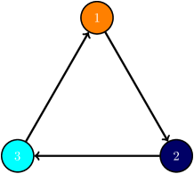
Figure 1: Illustration of the predation interaction rules among species in the rock-paper-scissors model.

III Spatial Patterns

We begin the numerical study by performing a single simulation for the cases $\kappa=0$ (the standard model), $\kappa=1$, $\kappa=3$, and $\kappa=5$. The realizations run in square lattices with $600^{2}$ sites for a timespan of $5000$ generations, assuming $p=2/3$ and $m=1/3$. The dynamics of the spatial patterns are shown in videos in Refs. Josinaldo Menezes (a, b, c, d). The snapshots depicted in the upper left, upper right, lower left, and lower right panels show the spatial configuration at the end of the simulations for $\kappa=0$, $\kappa=1$, $\kappa=3$, and $\kappa=5$, respectively. The colors follow the scheme in Fig. 1, where orange, dark blue, and cyan dots show individuals of species $1$, $2$, and $3$, respectively.

The aleatory distribution of individuals leads to a high predation rate in the initial stage of the simulation. In the standard model ($\kappa=0$), predators find and consume preys everywhere without resistance. The local species segregation continuously changes because of the cyclic predation interactions. For example, when a group of individuals of species $1$ appears, it is consumed and substituted by individuals of species $2$. The new spatial domain of species $2$ is, in its turn, destroyed by individuals of species $3$, that serve as food for species $1$. The consequence is the formation of irregular groups during the simulation, as shown in the upper left panel of Fig. 2. The video Josinaldo Menezes (a) shows the dynamics of the spatial patterns for the standard model during the entire simulation.

When antipredator behavior is considered, predation is no longer as likely probable to any predator. There is a local effect on the predation probability: the larger the prey group size, the more difficult it is to eat the prey. Because of this, predators that are close to conspecifics have more chances of devouring the prey. This accounts for the growth of the species spatial domains, leading to spiral patterns. As one sees in the upper right, lower left, and lower right panels of Fig. 2, $\kappa$ influences the spatial pattern formation. The more intense the prey’s resistance, the less likely predation to occur away from the boundaries of predator-dominated domains. Moreover, for higher $\kappa$, fewer predation interactions happen, increasing the effective mobility rate, and consequently, the spatial domain size (Avelino et al. (2012)). Videos Josinaldo Menezes (b) ($\kappa=1$), Josinaldo Menezes (c) ($\kappa=3$), and Josinaldo Menezes (d) ($\kappa=5$) show the dynamics of the species spatial segregation.

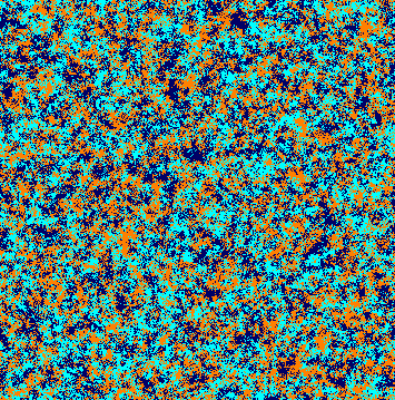
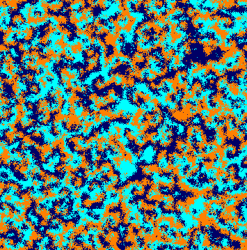
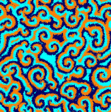
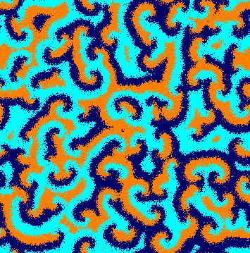
Figure 2: Snapshots of simulations of the rock-paper-scissors game illustrated in Fig. 1 running in square lattices with $600^{2}$ grid points. Each dot shows an individual according to the color scheme in Fig. 1. All simulations started from the same random initial conditions. The upper left, upper right, lower left, and lower right panels show the results for $\kappa=0$ (the standard model), $\kappa=1$, $\kappa=3$, and $\kappa=5$.

IV Dynamics of Species Densities

To quantify the population dynamics, we computed the spatial density $\rho$, defined as the fraction of the grid occupied by individuals of one species. Due to the cyclic tritrophic chain’s symmetry - inherent to the rock-paper-scissors model - the average spatial densities are the same for each species. Therefore, we concentrate only on the spatial density of species $1$, that is function of time $t$, i.e., $\rho(t)=I_{1}(t)/\mathcal{N}$.

The temporal changes in spatial densities of the simulations showed in Fig. 2 were depicted in Fig. 3. The grey line shows the dynamics of $\rho$ for the standard model (Josinaldo Menezes (a)), while the yellow, blue, and red lines represent the results for antipredator strength factor $\kappa=1$ (Josinaldo Menezes (b)), $\kappa=3$ (Josinaldo Menezes (c)), and $\kappa=5$(Josinaldo Menezes (d)), respectively. The outcomes show that the territorial dominance of species $i$ ($i=1,2,3$) is cyclic, as expected in the predator-prey models Lotka (1920); Volterra ((1931). The amplitude and frequency of the spatial densities increase for larger $\kappa$, resulting from the spiral pattern formation.

The species densities are also depicted in a ternary diagram in Fig. 4 for $\kappa=0$ (grey line), $\kappa=1$ (brown line), $\kappa=3$ (green line), and $\kappa=5$ (pink line). Even though the fluctuations of the species densities increase for larger $\kappa$, species coexist because the spatial domain average size is smaller than the grid size (Reichenbach et al. (2007); Avelino et al. (2018a)).

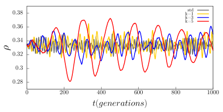
Figure 3: Temporal changes of spatial species densities $\rho$ in the simulations presented in Fig. 2. The grey, yellow, blue, and red lines represent the results for antipredator strength factor $\kappa=0$ (standard model), $\kappa=1$, $\kappa=3$, and $\kappa=5$, respectively.

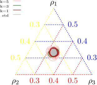
Figure 4: Ternary diagram of the species densities in the tritrophic systems presented in Fig. 2. The orbits for the cases $\kappa=0$, $\kappa=1$, $\kappa=3$, and $\kappa=5$, are showed by the grey, brown, green, and pink lines, respectively.

V Autocorrelation Function

The spatial autocorrelation function quantifies the species spatial segregation, measuring how individuals of the same species are spatially correlated. Again, we focus on computing the autocorrelation function of species $1$.

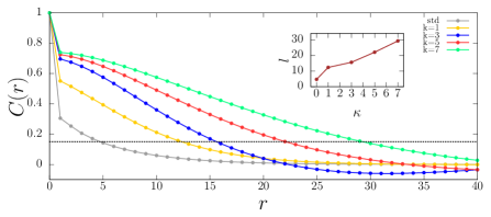
Figure 5: Autocorrelation functions $C(r)$. They grey, yellow, blue, red, and green lines show the outcomes for $\kappa=0$, $\kappa=1$, $\kappa=3$, $\kappa=5$, and $\kappa=7$, respectively. The horizontal dashed black line indicates the threshold assumed to calculate the characteristic length. The inset shows the characteristic length as a function of $\kappa$.

The autocorrelation function is computed from the inverse Fourier transform of the spectral density as

$$C(\vec{r}^{\prime})=\frac{\mathcal{F}^{-1}\{S(\vec{k})\}}{C(0)},$$ (2)

where $S(\vec{k})$ is given by

$$S(\vec{k})=\sum_{k_{x},k_{y}}\,\varphi(\vec{\kappa}),$$ (3)

with $\varphi(\vec{\kappa})$ being the following Fourier transform

$$\varphi(\vec{\kappa})=\mathcal{F}\,\{\phi(\vec{r})-\langle\phi\rangle\}.$$ (4)

The function $\phi(\vec{r})$ represents the spatial distribution of individuals of species $1$ ($\phi(\vec{r})=0$ and $\phi(\vec{r})=1$ indicate the absence and the presence of an individual of species $1$ in the the position $\vec{r}$ in the lattice, respectively).

The spatial autocorrelation function is computed as

$$C(r^{\prime})=\sum_{|\vec{r}^{\prime}|=x+y}\frac{C(\vec{r}^{\prime})}{min(2N-(x+y+1),(x+y+1)}.$$ (5)

Finally, we found the spatial domains’ scale for $C(l)=0.15$, where $l$ is the characteristic length.

Figure 5 shows how the spatial autocorrelation function changes in terms of the radial coordinate $r$, for various values of $\kappa$. The results were averaged from a set of $100$ simulations with lattices with $\mathcal{N}=300^{2}$ - each simulation started from different random initial conditions. The spatial configuration was captured after $3000$ generations, for $p=2/3$ and $m=1/3$. The yellow, blue, red, and green lines show the autocorrelation functions for $\kappa=1$, $\kappa=3$, $\kappa=5$, and $\kappa=7$, respectively in the upper panel. The grey line shows the autocorrelation function for the standard model, $\kappa=0$. The horizontal black line represents the threshold considered to calculate the length scale, $C(l)\,=\,0.15$. The inset shows the characteristic length in terms of $\kappa$. Accordingly, in the presence of the local effects of the antipredator behavior, the spatial clustering of individuals of the same species is remarkably augmented, reflecting the visualized effects in the spatial patterns.

VI Predation Risk

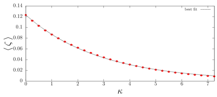
Figure 6: Mean predation risk as a function of the antipredator strength factor. The results were averaged from a set of $100$ simulations of squares lattices with $300^{2}$ points. The error bars shows the standard deviation.

Now, we aim to comprehend how collective antipredator behavior reduces the chances of an individual being killed. For this reason, we compute the predation risk $\zeta$. Because of the symmetry of the rock-paper-scissors model, individuals of every species have the same predation risk. We then focus on calculating $\zeta$ for species $1$.

We first count the total number of individuals of species $1$ at the beginning of each generation. Subsequently, we count how many individuals of species $1$ are consumed during the generation. The ratio between the number of preyed individuals and the initial amount is defined as the predation risk, $\zeta$. To avoid the noise inherent in the pattern formation period, we calculate the predation risk considering only the second half of the simulation. Besides, we averaged the results every $30$ generations.

To understand how the predation risk is sensitive to the antipredator strength factor $\kappa$, we run sets of $100$ realizations with different random initial conditions for each value of $\kappa$. The mean value of the predation risk, $\langle\zeta\rangle$ is depicted in Fig. 6 for $0\leq\kappa\leq 7.25$. The error bars show the standard deviation; $\kappa=0$ represents the standard model. We verified that the predation risk decreases exponentially when the antipredator strength factor grows. The best fit to the mean predation risk is given by

$$\langle\zeta\rangle\,=\,\langle\zeta_{0}\rangle\,e^{-\mu\,\kappa},$$ (6)

where $\langle\zeta_{0}\rangle=0.123\pm 3.7\times 10^{-4}$ is the predation risk in the standard model, whereas $\mu=0.35\pm 1.6\times 10^{-3}$. The fit shows the influence of the neighborhood on the predation risk. This means that $\mu$ computes the average antipredator effect caused by the prey group surrounding every predator.

VII Coexistence Probability

Finally, we aim to discover how antipredator behavior jeopardizes biodiversity. To this purpose, we performed $1000$ simulations in lattices with $120^{2}$ grid points for $0.05\,<\,m\,<\,0.95$ in intervals of $\Delta\,m\,=\,0.05$. The simulations started from different random initial conditions and run for a timespan of $120^{2}$ generations. Predation probability was set to $p\,=\,1-m$. Coexistence occurs if at least one individual of each species is present at the end of the simulation, $I_{i}(t=120^{4})\neq 0$ with $i=1,2,3$. Otherwise, the simulation results in extinction. The coexistence probability is the fraction of realizations resulting in coexistence.

We investigated how coexistence probability is affected by the antipredator strength factor $\kappa$. Figure  7 shows the results for various values of $\kappa$. Yellow, blue, red, and green lines show the coexistence probability for $\kappa=1$, $\kappa=3$, $\kappa=5$, and $\kappa=7$, respectively. As Fig. 7 indicates, the coexistence probability does not behave monotonically. This nonlinearity is a result of both the change of the spatial patterns resulting from the increase in $\kappa$ and the stochasticity caused by the different mobility probabilities Reichenbach et al. (2007).

For $m<0.55$, species biodiversity is more threatened when $\kappa=3$, while $m\geq 0.55$, the chances of all species persisting is lower for $\kappa=7$.

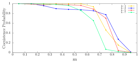
Figure 7: Coexistence probability as a function of the mobility probability $m$. The yellow, blue, red, and green lines show the results for $\kappa=1$, $\kappa=3$, $\kappa=3$, and $\kappa=7$, respectively. The results were obtained by running $1000$ simulations in lattices with $120^{2}$ grid points running until $120^{2}$

generations.

VIII Comments and Conclusions

We studied a tritrophic predator-prey system described by the nonhierarchical cyclic rock-paper-scissors game. In our model, collective behavior is responsible for the prey group’s opposition against a predator. Considering that the predation probability decreases exponentially with the prey group size and the antipredator strength, we performed a series of stochastic numerical simulations to understand the effects on the spatial pattern formation and species spatial densities. We also investigated the impact on predation risks and the coexistence probability.

Our main result shows that collective antipredator behavior leads to spiral pattern formation. Here, the Lotka-Volterra implementation of the rock-paper-scissors model shows the presence of spiral waves in on-lattice simulations. In Ref. Peltomäki and Alava (2008), the authors claim that this is not possible when a conservation law for the total number of individuals is assumed, nor is it likely to form any other visible spatial pattern (this was confirmed in our simulations for $\kappa=0$). The authors also claimed that spiral patterns only appear whether the total number of individuals on the lattice is no longer conserved (Peltomäki and Alava (2008)), the so-called May-Leonard implementation. In this case, besides individuals of species $1$, $2$, and $3$, empty spaces are also considered on the lattice (see Refs. Reichenbach et al. (2007); Avelino et al. (2012); Menezes et al. (2019); Avelino et al. (2019)). Indeed, for the Lotka-Volterra implementation, spiral patterns were observed exclusively in off-lattice simulations (Avelino et al. (2018b); Ni et al. (2010a, b)). Here, the spiral patterns result from the influence of the group size on local antipredator behavior: individuals on the borders between predator-dominated and prey-dominated are more likely to succeed in preying. This is similar to the May-Leonard implementation, where individuals need empty spaces, mostly present on domain boundaries, to reproduce.

Our findings also show how predation risk decreases exponentially with the antipredator strength factor. More, we verified that the collective antipredator behavior might jeopardize biodiversity for higher mobility probabilities. Our outcomes help to understand how regional conditions affect predators’ performance and, consequently, change population dynamics in cyclic models. The results may also shed light on investigations of complex systems in other areas of nonlinear science.

IX Acknowledgments

We thank Beatriz Moura and Enzo Rangel for enlightening discussions. We acknowledge ECT/UFRN, CNPQ/Fapern and IBED-Universiteit van Amsterdam for financial support.

References

- Begon et al. (2006) M. Begon, C. R. Townsend, and J. L. Harper, Ecology: from individuals to ecosystems (Blackwell Publishing, Oxford, 2006).
- Purvis and Hector (2000) A. Purvis and A. Hector, Nature 405, 212 (2000).
- Buchholz (2007) R. Buchholz, Trends in Ecology & Evolution 22, 401 (2007), ISSN 0169-5347.
- Kerr et al. (2002) B. Kerr, M. A. Riley, M. W. Feldman, and B. J. M. Bohannan, Nature 418, 171 (2002).
- Kirkup and Riley (2004) B. C. Kirkup and M. A. Riley, Nature 428, 412 (2004).
- Durret and Levin (1997) R. Durret and S. Levin, J. Theor. Biol. 185, 165 (1997).
- Sinervo and Lively (1996) B. Sinervo and C. M. Lively, Nature 380, 240 (1996).
- Volkov et al. (2007) I. Volkov, J. R. Banavar, S. P. Hubbell, and A. Maritan, Nature 450, 45 (2007).
- Szolnoki et al. (2020) A. Szolnoki, B. F. de Oliveira, and D. Bazeia, EPL (Europhysics Letters) 131, 68001 (2020).
- Szolnoki et al. (2014) A. Szolnoki, M. Mobilia, L.-L. Jiang, B. Szczesny, A. M. Rucklidge, and M. Perc, Journal of The Royal Society Interface 11, 20140735 (2014).
- Lotka (1920) A. J. Lotka, Journal of the American Chemical Society 42, 1595 (1920).
- Volterra ((1931) V. Volterra, Lecons dur la Theorie Mathematique de la Lutte pour la Vie (Gauthier-Villars, Paris, (1931)), ed.
- Reichenbach et al. (2007) T. Reichenbach, M. Mobilia, and E. Frey, Nature 448, 1046 (2007).
- Avelino et al. (2012) P. P. Avelino, D. Bazeia, L. Losano, J. Menezes, and B. F. Oliveira, Phys. Rev. E 86, 036112 (2012).
- Menezes et al. (2019) J. Menezes, B. Moura, and T. A. Pereira, Europhysics Letters 126, 18003 (2019).
- Peltomäki and Alava (2008) M. Peltomäki and M. Alava, Phys. Rev. E 78, 031906 (2008).
- Cheng et al. (2018) H. Cheng, N. Yao, Z.-G. Huang, J. Park, Y. Do, and Y.-C. Lai, Scientific Reports 8, 2045 (2018).
- Avelino et al. (2014) P. P. Avelino, D. Bazeia, L. Losano, J. Menezes, and B. F. de Oliveira, Phys. Rev. E 89, 042710 (2014).
- Pereira et al. (2018) T. A. Pereira, J. Menezes, and L. Losano, Intern. J. of Mod., Sim. and Sci. Comp. 9, 1850046 (2018).
- Avelino et al. (2019) P. P. Avelino, J. Menezes, B. F. de Oliveira, and T. A. Pereira, Phys. Rev. E 99, 052310 (2019).
- Fraenkel and Gunn (1941) G. S. Fraenkel and D. L. Gunn, The American Naturalist 75, 604 (1941).
- Cormont et al. (2011) A. Cormont, A. H. Malinowska, O. Kostenko, V. Radchuk, L. Hemerik, M. F. WallisDeVries, and J. Verboom, Biodiversity and Conservation 20, 483 (2011).
- Altieri (2008) A. H. Altieri, Ecology 89, 2808 (2008).
- Whitlow et al. (2003) W. L. Whitlow, N. A. Rice, and C. Sweeney, Biological Invasions 5, 23 (2003).
- Moura and Menezes (2021) B. Moura and J. Menezes, Scientific Reports 11, 6413 (2021).
- Caro (2005) T. Caro, Antipredator Defenses in Birds and Mammals (The University of Chicago Press., London, 2005).
- Humphreys and Ruxton (2018) R. K. Humphreys and G. D. Ruxton, Behav. Ecol. and Sociol. 72, 22 (2018).
- Balaa and Blouin-Demers (2011) R. E. Balaa and G. Blouin-Demers, J. Appl. Ichthyol. 27, 1052 (2011).
- Choh et al. (2010) Y. Choh, M. Uefune, and J. Takabayashi, Exp. App. Acarol. 50, 1 (2010).
- Faraji et al. (2001) F. F. Faraji, A. Janssen, and M. W. Sabelis, Exp. App. Acarol. 25, 613–623 (2001).
- Saito et al. (2008) Y. Saito, A. R. Chittenden, K. Mori, K. Ito, and A. Yamauchi, Behav. Ecol, Sociobiol. 63, 33 (2008).
- Lemos et al. (2010) F. Lemos, R. A. Sarmento, A. Pallini, C. R. Dias, M. W. Sabelis, and A. Janssen, Exp. Appl. Acarol. 52, 1 (2010).
- Dias et al. (2016) C. R. Dias, A. M. G. Bernado, J. Mecalha, C. W. C. Freitas, R. A. Sarmento, A. Pallini, and A. Janssen, Exp. Appl. Acarol. 69, 263 (2016).
- Dittmann and Schausberger (2017) L. Dittmann and P. Schausberger, Sci. Rep. 7, 10609 (2017).
- Downes and Hoefer (2004) S. Downes and A. M. Hoefer, Animal Behaviour 67, 485 (2004).
- Berger (1978) J. Berger, Behav. Ecol. Sociobiol. 4, 91 (1978).
- Mori and Saito (2004) K. Mori and Y. Saito, Behav. Ecol, Sociobiol. 56, 201 (2004).
- Cazaubiel et al. (2017) A. Cazaubiel, A. F. Lütz, and J. J. Arenzon, J. Theor. Biol. 430, 45 (2017).
- Josinaldo Menezes (a) Josinaldo Menezes, Standard lotka-volterra implementation of the rock-paper-scissors model, [YouTube video], URL https://youtu.be/21_YjeNvK3s.
- Josinaldo Menezes (b) Josinaldo Menezes, Antipredator behaviour rock-paper-scissors model - k=1, [YouTube video], URL https://youtu.be/6uI58Q-2vMU.
- Josinaldo Menezes (c) Josinaldo Menezes, Antipredator behaviour rock-paper-scissors model - k=3, [YouTube video], URL https://youtu.be/Wc758xSQIEs.
- Josinaldo Menezes (d) Josinaldo Menezes, Antipredator behaviour rock-paper-scissors model - k=5, [YouTube video], URL https://youtu.be/9ggvljOK6sI.
- Avelino et al. (2018a) P. P. Avelino, D. Bazeia, L. Losano, J. Menezes, B. F. de Oliveira, and M. A. Santos, Phys. Rev. E 97, 032415 (2018a).
- Avelino et al. (2018b) P. P. Avelino, D. Bazeia, L. Losano, J. Menezes, and B. F. de Oliveira, EPL (Europhysics Letters) 121, 48003 (2018b).
- Ni et al. (2010a) X. Ni, R. Yang, W.-X. Wang, Y.-C. Lai, and C. Grebogi, Chaos: An Interdisciplinary Journal of Nonlinear Science 20, 045116 (2010a).
- Ni et al. (2010b) X. Ni, W.-X. Wang, Y.-C. Lai, and C. Grebogi, Phys. Rev. E 82, 066211 (2010b).