OpenICS: Open Image Compressive Sensing Toolbox and Benchmark

Jonathan Zhao^*, Matthew Westerham^*, Mark Lakatos-Toth^*, Zhikang Zhang^*, Avi Moskoff, Fengbo Ren
* equally contribute Parallel Systems and Computing Laboratory
Arizona State University
Tempe, USA
jjzhao@asu.edu, mkweste1@asu.edu, mlakato1@asu.edu, zzhan362@asu.edu, amoskoff@asu.edu, renfengbo@asu.edu

Abstract

We present OpenICS, an image compressive sensing toolbox that includes multiple image compressive sensing and reconstruction algorithms proposed in the past decade. Due to the lack of standardization in the implementation and evaluation of the proposed algorithms, the application of image compressive sensing in the real-world is limited. We believe this toolbox is the first framework that provides a unified and standardized implementation of multiple image compressive sensing algorithms. In addition, we also conduct a benchmarking study on the methods included in this framework from two aspects: reconstruction accuracy and reconstruction efficiency. We wish this toolbox and benchmark can serve the growing research community of compressive sensing and the industry applying image compressive sensing to new problems as well as developing new methods more efficiently. Code and models are available at https://github.com/PSCLab-ASU/OpenICS. The project is still under maintenance, and we will keep this document updated.

Index Terms:

compressive sensing, computer vision, machine learning, signal processing

I Introduction

Compressive sensing is a signal sensing technique that performs the sensing and compression of signals simultaneously to reduce the sensing cost without losing information. Over the past decade, there is a wide variety of image compressive sensing reconstruction methods proposed. However, due to the lack of standardization in the implementation and evaluation of the proposed algorithms, the application of image compressive sensing in the real-world is still limited. Towards the goal of efficient deployment and evaluation of image compressive sensing, we build OpenICS which is an image compressive sensing toolbox containing multiple image compressive sensing reconstruction methods implemented in a unified interface and structure.

Major features of OpenICS are 1. Unified interface. We rewrite the code of multiple image compressive sensing algorithms to build a unified interface for all the methods. This unified design greatly improves the usability and availability of our toolbox. 2. Modular design. Each method locates in a separate folder, and there is no cross-dependency between different methods. This modular design improves the reusability of our toolbox. 3. Out-of-the-box usage. Our toolbox contains the most representative methods of image compressive sensing methods. See Section 2 for the full list.

In addition to the toolbox we implemented, we also propose a benchmark to evaluate all the methods included in the toolbox from two aspects: reconstruction accuracy and reconstruction speed. The benchmark results include the performance of all the methods evaluated on six different datasets and five different compression ratios. We believe our benchmark is the most complete benchmark in the domain of image compressive sensing so far in terms of the variety of datasets and the range of compression ratios.

Our contribution are summarized as follows:

1. We provide a toolbox in the domain of image compressive sensing that consists of multiple most representative algorithms in this domain. The toolbox has a unified interface, modular design, and it can be used out of box.

2. We propose a benchmark in the domain of image compressive sensing and use it to evaluate the methods included in our toolbox. It is by far the most complete benchmark in the domain of image compressive sensing in terms of the variety of datasets and the range of compression ratios.

II Methods Included

OpenICS contains implementations of multiple image CS reconstruction methods. Based on whether the method is data-dependent, we divide implemented methods into two categories: Model-based methods and data-driven methods.

II-A Model-based Methods

Model-based methods use pre-defined models based on prior knowledge of the signals to perform the reconstruction. The included model-based methods are listed and summarized in table I.

L1[1]: The first reconstruction methods in the domain of compressive sensing(Only the total-variation-based methods are currently implemented).

NLR-CS[2]: A reconstruction method based on non-local low-rank regularization.

TVAL-3[3]: An efficient image reconstruction method based on total variation minimization.

D-AMP[4]: An reconstruction method based on model-based image denoising algorithms.

II-B Data-driven Methods

Data-driven methods do not rely on pre-defined models of signals. Instead, they use neural networks to model the images and perform the reconstruction tasks. The included data-driven methods are listed below.

ReconNet[5]: An end-to-end reconstruction network based on convolutional neural networks.

LDAMP[6]: An end-to-end reconstruction network built from the unrolled iterative image denoising process by replacing the model-based image denoisers with neural-network-based denoisers.

ISTA-Net[7]: An end-to-end reconstruction network built by unrolling the conventional iterative shrinkage-thresholding algorithm.

LAPRAN[8]: An end-to-end reconstruction network based on deep laplacian pyramid neural networks.

CSGM[9]: An iterative reconstruction method based on generative adversial neural network.

CSGAN[10]: A variant of CSGM method enhanced by meta-learning to improve reconstruction speed.

Methods	Data dependent	Running process	Platform
L1	No	Iterative	CPU
TVAL-3	No	Iterative	CPU
NLR-CS	No	Iterative	CPU
D-AMP	No	Iterative	CPU
ReconNet	Yes	End-to-end	GPU
ISTA-Net	Yes	End-to-end	GPU
LDAMP	Yes	End-to-end	GPU
CSGM	Yes	Iterative	GPU
LAPRAN	Yes	End-to-end	GPU
CSGAN	Yes	Iterative	GPU

TABLE I: List of methods included in OpenICS

III Architecture

III-A Toolbox Structure

There are two programing languages used to implement all the methods. L1, NLR-CS, TVAL-3, D-AMP are implemented in Matlab. ReconNet, ISTA-Net, LAPRAN are implemented in Python with Pytorch[11]. CSGM, CSGAN, LDAMP are implemented in Python with Tensorflow[12].

We provide a unified interface to run all the methods. Specifically, the common parameters of all methods are listed as follows:

1.

dataset: the name of dataset to be used
2.

input_channel: number of channels training/testing images have
3.

input_width: width of training/testing images
4.

input_height: height of training/testing images
5.

m: number of measurements/outputs of sensing matrix
6.

n: number of inputs to sensing matrix

Besides, there are method-specific parameters that are included in a container-like object called ”specifics”. In python, it is a dictionary with its keys as parameter names and its values as actual parameters. In Matlab, it is a structure array with its field names as parameter names, and its field values are the parameters.

We also provide the functionality to directly call certain methods from the main interface. The parameters of the main interface are listed below:

1.

sensing: method of sensing
2.

reconstruction: method of reconstruction
3.

stage: training or testing(model-based methods do not have this parameter)
4.

default: will use default parameters if it’s true. Will override other parameters set manually.
5.

dataset: same as method’s corresponding parameter.
6.

input_channel: same as method’s corresponding parameter.
7.

input_width: same as method’s corresponding parameter.
8.

input_height: same as method’s corresponding parameter.
9.

m: same as method’s corresponding parameter.
10.

n: same as method’s corresponding parameter.
11.

specifics: specific parameter settings of chosen reconstruction method. Will be passed to the actual method.

Given an image to be sensed and reconstructed, for model-based methods, it can be directly reconstructed by calling the main function of specific methods. For data-driven methods, the networks of specific methods have to be trained first. We provide pre-trained networks of each method at five compression ratios(2,4,8,16,32) on six datasets. We also provide the functionality of training new networks on new datasets and compression ratios from scratch.

More details regarding how to use our code are listed in the main page of our Github repository(https://github.com/PSCLab-ASU/OpenICS).

IV Benchmarks

IV-A Benchmark Design

Dataset. We use six widely used datasets to evaluate all the methods in benchmark. They are MNIST[13], CIFAR10[14], CIFAR10(grayscaled), CELEBA[15], Bigset, Bigset(grayscaled). Bigset stands for a manually composed dataset. It was initially used in [16, 17, 18] in the domain of single image super-resolution. Later it was used in LAPRAN[8] for image compressive sensing. The training set of Bigset was composed of 91 images from [19] and 200 images from the BSD[20] dataset. The 291 images are augmented (rotation and flip) and cut into 228688 patches as training samples. The testing set of Bigset consists of image patches from Set5[21] and Set14[22] with same patch size. For MNIST, CIFAR10, CIFAR10(gray), the image size of samples is 32x32. For CELEBA, Bigset(gray) and Bigset, the image size of samples is 64x64.

Compression ratios. We take five different compression ratios to evaluate each method: 2,4,8,16,32. The compression is always performed channel-wise, i.e., for colored images(with RGB color channels), we perform the compression over each channel seperately. The measurements of all three channels are then grouped together for subsequent reconstruction. The training procedure of each data-driven method is almost the same as the original training guideline provided by the original authors. The discrepancy is detailed in our github repository.

Metrics. We evaluate all the methods from two aspects: reconstruction accuracy and reconstruction speed. The reconstruction accuracy is quantified with two metrics: PSNR(0-48) and SSIM(0-1) between reconstructed images and original images in the testing set. Higher values indicate higher accuracy. For each experiment we conduct, the reported results are the averaged values of both metrics over all the samples of the corresponding testing set. The reconstruction speed is quantified with the number of images reconstructed per second. This value is averaged over all the samples in the testing set as well.

Benchmark calculation. After obtaining the all raw benchmark results of each method(total of $6\text{\ datasets}\times 5\text{\ compression ratios}\times 3\text{\ metrics}=90\text{\ raw results}$ ), we use the following equation to calculate the final benchmark score:

score=\sum_{i=1}^{90}w_{dataset}*w_{cr}*w_{metric}*\bar{v}_{i}

(1)

$\bar{v}_{i}$ is the ith normalized raw experiment result. Due to the different value ranges of each metric, we have to normalize the raw values to 0-100 range to avoid the dominance of one metric over the others. The function used to normalize PSNR values is $\bar{v}=10^{\frac{v}{48}-1}*100$ . The function used to normalize SSIM values is $\bar{v}=10^{v-1}*100$ . The function used to normalize reconstruction speed values is $\bar{v}=\frac{100}{1+1/log(1+v)}$ .

$w_{dataset}$ is the weight of the corresponding dataset of $v_{i}$ . Different weights are assigned to different datasets according to their relative complexity in reconstruction compared with other datasets. The relative complexity is determined based on the results reported in literatures[1, 3, 2, 4, 5, 7, 6, 8, 9, 10] in the domain of image compressive sensing.

$w_{cr}$ is the weight of the corresponding compression ratio of $v_{i}$ . Since images compressed at higher compression ratios are more difficult to reconstruct than images compressed at lower compression ratios, we assign higher weights to higher compression ratios.

$w_{metric}$ is the weight of corresponding metric of $v_{i}$ . we assign different weights to different metrics as $\text{PSNR}:\text{SSIM}:\text{Speed}=1:1:2$ . As such, there is no bias between reconstruction accuracy and reconstruction speed. One can specify own weights to different metrics to make the score reflects one’s own preferences.

The actual weights are listed in table II,table III and table IV.

Dataset	Weight
MNIST	1/21
CelebA	4/21
CIFAR10	3/21
CIFAR10 Gray	2/21
Bigset	6/21
Bigset Gray	5/21

TABLE II: Weights of Datasets

Compression ratio	Weight
2	1/31
4	2/31
8	4/31
16	8/31
32	16/31

TABLE III: Weights of compression ratios

Metric	Weight
PSNR	1/4
SSIM	1/4
Reconstruction speed	1/2

TABLE IV: Weights of metrics

IV-B Benchmark Results

The raw benchmark results are listed in Table VI,VII,VIII,IX,X,XI,XII,XIII,XIV and XV in the appendix. The benchmark score of each method is shown in Table V and Fig 1.

Method	Speed	Accuracy	Score
LDAMP	30.25	17.21	47.46
ISTA-Net	30.02	20.69	50.71
CSGAN	32.58	19.03	51.61
LAPRAN	34.69	23.60	58.30
CSGM	4.75	13.07	17.82
ReconNet	37.00	19.15	56.15
TVAL-3	18.43	18.92	37.35
L1	3.78	19.69	23.46
D-AMP	2.35	21.83	24.19
NLR-CS	1.69	20.35	22.04

TABLE V: The benchmark scores

Refer to caption — Figure 1: The benchamark scores

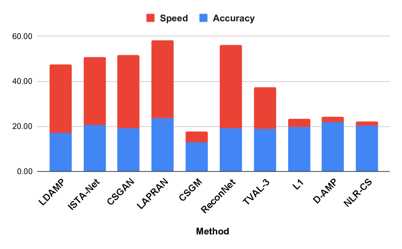
LAPRAN has the highest benchmark score due to its prominent performance in accuracy and speed. LDAMP has the highest performance in accuracy but bad performance in speed due to its heavyweight design of network structure(more than 200 neural layers). ReconNet has the highest performance in reconstruction speed due to its lightweight design in structure(only seven layers), but its performance in accuracy is limited as well. In general, model-based methods have lower performance on both accuracy and speed than data-driven methods due to their static, pre-defined signal prior and iterative running process. CSGM is a special case in data-driven methods. The unsatisfying performance in accuracy is due to the GAN model it uses, which is DCGAN[23] proposed in 2015. Over the past few years, there have been more successful GAN models proposed, such as StyleGAN[24] that has much higher performance in modeling signals from data, which may improve the performance of CSGM if it is used. For all the model-based methods, NLR-CS and D-AMP have higher performance in reconstruction accuracy but lower performance in reconstruction speed compared with the other two methods.

To conclude, in general, data-driven methods achieve the highest performance in terms of accuracy and performance. With enough training data and hardware platforms that have sufficient computation capacity, one should always choose end-to-end data-driven methods. If there is no sufficient data, one should choose model-based methods that have the highest reconstruction accuracy. If the reconstruction speed is a critical factor to consider as well, TVAL-3 has a significantly higher reconstruction speed than other model-based methods and comparable reconstruction accuracy to other methods.

Acknowledgment

This work is supported by the Research Experiences for Undergraduates (REU) funding of an NSF grant (IIS/CPS-1652038) and the Fulton Undergraduate Research Initiative (FURI) program at Arizona State University. Part of the NVIDIA GPUs used for this work was donated by NVIDIA Corporation. The CPU servers used for this work were donated by Intel Corporation.

References

[1] E. Candes and J. Romberg, “l1-magic: Recovery of sparse signals via convex programming,” URL: www. acm. caltech. edu/l1magic/downloads/l1magic. pdf, vol. 4, p. 14, 2005.
[2] W. Dong, G. Shi, X. Li, Y. Ma, and F. Huang, “Compressive sensing via nonlocal low-rank regularization,” IEEE transactions on image processing, vol. 23, no. 8, pp. 3618–3632, 2014.
[3] C. Li, W. Yin, H. Jiang, and Y. Zhang, “An efficient augmented lagrangian method with applications to total variation minimization,” Computational Optimization and Applications, vol. 56, no. 3, pp. 507–530, 2013.
[4] C. A. Metzler, A. Maleki, and R. G. Baraniuk, “From denoising to compressed sensing,” IEEE Transactions on Information Theory, vol. 62, no. 9, pp. 5117–5144, 2016.
[5] K. Kulkarni, S. Lohit, P. Turaga, R. Kerviche, and A. Ashok, “Reconnet: Non-iterative reconstruction of images from compressively sensed measurements,” in Proceedings of the IEEE Conference on Computer Vision and Pattern Recognition, 2016, pp. 449–458.
[6] C. A. Metzler, A. Mousavi, and R. G. Baraniuk, “Learned d-amp: Principled neural network based compressive image recovery,” arXiv preprint arXiv:1704.06625, 2017.
[7] J. Zhang and B. Ghanem, “Ista-net: Interpretable optimization-inspired deep network for image compressive sensing,” in Proceedings of the IEEE conference on computer vision and pattern recognition, 2018, pp. 1828–1837.
[8] K. Xu, Z. Zhang, and F. Ren, “Lapran: A scalable laplacian pyramid reconstructive adversarial network for flexible compressive sensing reconstruction,” in Proceedings of the European Conference on Computer Vision (ECCV), 2018, pp. 485–500.
[9] A. Bora, A. Jalal, E. Price, and A. G. Dimakis, “Compressed sensing using generative models,” in International Conference on Machine Learning. PMLR, 2017, pp. 537–546.
[10] Y. Wu, M. Rosca, and T. Lillicrap, “Deep compressed sensing,” in International Conference on Machine Learning. PMLR, 2019, pp. 6850–6860.
[11] A. Paszke, S. Gross, F. Massa, A. Lerer, J. Bradbury, G. Chanan, T. Killeen, Z. Lin, N. Gimelshein, L. Antiga et al., “Pytorch: An imperative style, high-performance deep learning library,” arXiv preprint arXiv:1912.01703, 2019.
[12] M. Abadi, P. Barham, J. Chen, Z. Chen, A. Davis, J. Dean, M. Devin, S. Ghemawat, G. Irving, M. Isard et al., “Tensorflow: A system for large-scale machine learning,” in 12th $\{$ USENIX $\}$ symposium on operating systems design and implementation ( $\{$ OSDI $\}$ 16), 2016, pp. 265–283.
[13] Y. LeCun, L. Bottou, Y. Bengio, and P. Haffner, “Gradient-based learning applied to document recognition,” Proceedings of the IEEE, vol. 86, no. 11, pp. 2278–2324, 1998.
[14] A. Krizhevsky, G. Hinton et al., “Learning multiple layers of features from tiny images,” 2009.
[15] Z. Liu, P. Luo, X. Wang, and X. Tang, “Deep learning face attributes in the wild,” in Proceedings of International Conference on Computer Vision (ICCV), December 2015.
[16] J. Kim, J. Kwon Lee, and K. Mu Lee, “Accurate image super-resolution using very deep convolutional networks,” in Proceedings of the IEEE conference on computer vision and pattern recognition, 2016, pp. 1646–1654.
[17] W.-S. Lai, J.-B. Huang, N. Ahuja, and M.-H. Yang, “Deep laplacian pyramid networks for fast and accurate super-resolution,” in Proceedings of the IEEE conference on computer vision and pattern recognition, 2017, pp. 624–632.
[18] S. Schulter, C. Leistner, and H. Bischof, “Fast and accurate image upscaling with super-resolution forests,” in Proceedings of the IEEE conference on computer vision and pattern recognition, 2015, pp. 3791–3799.
[19] J. Yang, J. Wright, T. S. Huang, and Y. Ma, “Image super-resolution via sparse representation,” IEEE transactions on image processing, vol. 19, no. 11, pp. 2861–2873, 2010.
[20] P. Arbelaez, M. Maire, C. Fowlkes, and J. Malik, “Contour detection and hierarchical image segmentation,” IEEE transactions on pattern analysis and machine intelligence, vol. 33, no. 5, pp. 898–916, 2010.
[21] M. Bevilacqua, A. Roumy, C. Guillemot, and M. L. Alberi-Morel, “Low-complexity single-image super-resolution based on nonnegative neighbor embedding,” 2012.
[22] R. Zeyde, M. Elad, and M. Protter, “On single image scale-up using sparse-representations,” in International conference on curves and surfaces. Springer, 2010, pp. 711–730.
[23] A. Radford, L. Metz, and S. Chintala, “Unsupervised representation learning with deep convolutional generative adversarial networks,” arXiv preprint arXiv:1511.06434, 2015.
[24] T. Karras, S. Laine, and T. Aila, “A style-based generator architecture for generative adversarial networks,” in Proceedings of the IEEE/CVF Conference on Computer Vision and Pattern Recognition, 2019, pp. 4401–4410.

V Appendix

	Compression ratio	PSNR	SSIM	Reconstruction per second
MNIST	2	47.9998	0.9997	27.5482
MNIST	4	47.5808	0.9994	34.6021
MNIST	8	39.8992	0.9965	34.9650
MNIST	16	30.8985	0.9751	34.7222
MNIST	32	16.2898	0.5901	34.3643
CelebA	2	41.1183	0.9911	23.4192
CelebA	4	32.0614	0.9459	27.5482
CelebA	8	27.5465	0.8723	30.9598
CelebA	16	23.592	0.7415	33.5570
CelebA	32	17.5607	0.3732	32.5733
CIFAR10	2	35.1695	0.9748	35.2113
CIFAR10	4	28.5017	0.9052	35.4610
CIFAR10	8	22.7743	0.7285	33.5570
CIFAR10	16	18.8613	0.498	34.6021
CIFAR10	32	13.7782	0.1406	34.1297
CIFAR10(Gray)	2	34.3648	0.9713	32.5733
CIFAR10(Gray)	4	27.8835	0.8945	33.0033
CIFAR10(Gray)	8	23.2726	0.7499	34.4828
CIFAR10(Gray)	16	16.6404	0.3471	35.2113
CIFAR10(Gray)	32	12.2314	0.0701	35.0877
Bigset	2	38.4191	0.9432	23.9234
Bigset	4	34.3927	0.8936	29.1545
Bigset	8	30.9195	0.8096	29.2398
Bigset	16	27.608	0.7055	34.3643
Bigset	32	17.3593	0.1853	33.2226
Bigset(Gray)	2	38.5702	0.9508	22.8311
Bigset(Gray)	4	34.5885	0.8956	27.3224
Bigset(Gray)	8	31.0164	0.808	30.1205
Bigset(Gray)	16	28.3581	0.7207	33.4448
Bigset(Gray)	32	17.283	0.178	35.5872

TABLE VI: Benchmark results of LDAMP

Dataset	Compression ratio	PSNR	SSIM	Reconstruction per second
MNIST	2	47.99	0.9999	93.4579
MNIST	4	44.27	0.9988	55.2486
MNIST	8	35.12	0.9907	75.7576
MNIST	16	27.31	0.9532	75.7576
MNIST	32	19.76	0.7747	82.6446
CelebA	2	37.43	0.9798	11.9190
CelebA	4	31.14	0.9297	14.3062
CelebA	8	27.07	0.8499	4.8170
CelebA	16	23.77	0.7406	7.3475
CelebA	32	21.13	0.6295	17.5439
CIFAR10	2	34.12	0.9703	30.1205
CIFAR10	4	27.66	0.8932	33.2226
CIFAR10	8	23.41	0.7632	31.4465
CIFAR10	16	20.25	0.5979	25.9067
CIFAR10	32	17.95	0.435	26.3852
CIFAR10(Gray)	2	33.63	0.9679	138.8889
CIFAR10(Gray)	4	27.46	0.8886	68.0272
CIFAR10(Gray)	8	23.15	0.7501	75.1880
CIFAR10(Gray)	16	20.25	0.5911	81.3008
CIFAR10(Gray)	32	18.13	0.4406	86.2069
Bigset	2	37.28	0.9393	15.8479
Bigset	4	33	0.8686	19.5313
Bigset	8	29.88	0.7823	22.0751
Bigset	16	27.03	0.682	25.6410
Bigset	32	24.67	0.5864	29.7619
Bigset(Gray)	2	38.49	0.95	57.8035
Bigset(Gray)	4	34.06	0.8874	76.9231
Bigset(Gray)	8	30.69	0.8007	82.6446
Bigset(Gray)	16	27.66	0.7035	74.0741
Bigset(Gray)	32	25.16	0.6074	65.3595

TABLE VII: Benchmark results of ISTA-Net

Dataset	Compression ratio	PSNR	SSIM	Reconstruction per second
MNIST	2	29.2126	0.9640	118.4133
MNIST	4	30.5120	0.9563	120.9862
MNIST	8	29.1593	0.9558	123.8261
MNIST	16	25.2426	0.9275	122.9381
MNIST	32	21.3493	0.8455	121.1784
CelebA	2	20.2156	0.8108	71.2754
CelebA	4	17.7137	0.6881	73.5295
CelebA	8	18.0141	0.7477	71.7567
CelebA	16	21.0598	0.8439	73.0777
CelebA	32	21.5447	0.8538	71.7036
CIFAR10	2	19.8350	0.8110	70.4578
CIFAR10	4	21.6027	0.8646	69.8564
CIFAR10	8	21.7896	0.8692	71.6831
CIFAR10	16	21.2262	0.8506	72.7173
CIFAR10	32	19.7638	0.7946	71.1875
CIFAR10(Gray)	2	23.4110	0.7581	75.6761
CIFAR10(Gray)	4	22.8502	0.7318	75.1091
CIFAR10(Gray)	8	21.7888	0.6794	74.7101
CIFAR10(Gray)	16	19.7298	0.5493	74.7030
CIFAR10(Gray)	32	18.1149	0.4288	74.9074
Bigset	2	18.1686	0.5370	72.5171
Bigset	4	16.3798	0.3874	80.3709
Bigset	8	17.6498	0.4811	72.8396
Bigset	16	21.4860	0.6384	72.8716
Bigset	32	21.0166	0.6326	66.1600
Bigset(Gray)	2	18.2207	0.2187	70.1563
Bigset(Gray)	4	21.5229	0.3874	68.3210
Bigset(Gray)	8	23.2503	0.5378	71.6273
Bigset(Gray)	16	23.5321	0.5401	72.4786
Bigset(Gray)	32	22.8348	0.5089	71.2181

TABLE VIII: Benchmark results of CSGAN

Dataset	Compression ratio	PSNR	SSIM	Reconstruction per second
MNIST	2	32.0483	0.9156	223.1187
MNIST	4	32.1388	0.9869	221.9279
MNIST	8	26.5582	0.954	222.8450
MNIST	16	23.3674	0.8691	229.3073
MNIST	32	19.7423	0.7701	219.0102
CelebA	2	29.4438	0.975	137.9121
CelebA	4	33.2433	0.9888	150.3084
CelebA	8	28.9183	0.9698	146.9329
CelebA	16	26.2793	0.9483	151.5757
CelebA	32	23.1517	0.8969	151.6358
CIFAR10	2	31.6029	0.9862	174.7553
CIFAR10	4	27.808	0.9674	225.8276
CIFAR10	8	25.4534	0.9428	227.8823
CIFAR10	16	22.262	0.8844	230.9234
CIFAR10	32	19.852	0.7874	214.7841
CIFAR10(Gray)	2	25.7358	0.8669	141.5323
CIFAR10(Gray)	4	23.6409	0.7804	219.8296
CIFAR10(Gray)	8	21.621	0.6675	229.1173
CIFAR10(Gray)	16	19.6054	0.5293	223.8697
CIFAR10(Gray)	32	18.0317	0.3887	232.5259
Bigset	2	30.7518	0.9314	30.5301
Bigset	4	30.2502	0.9214	34.1619
Bigset	8	28.3798	0.881	36.4556
Bigset	16	27.3575	0.8539	34.5518
Bigset	32	24.035	0.7489	41.8374
Bigset(Gray)	2	30.5937	0.8376	35.3011
Bigset(Gray)	4	30.2819	0.8125	41.4439
Bigset(Gray)	8	27.0031	0.7037	32.2543
Bigset(Gray)	16	25.1241	0.6216	41.1410
Bigset(Gray)	32	23.6821	0.5611	44.2111

TABLE IX: Benchmark results of LAPRAN

Dataset	Compression ratio	PSNR	SSIM	Reconstruction per second
MNIST	2	22.6164	0.8978	2.0329
MNIST	4	22.4511	0.8923	2.3868
MNIST	8	21.9578	0.8742	2.6208
MNIST	16	20.6622	0.8215	2.6924
MNIST	32	17.7698	0.6985	2.8841
CelebA	2	21.0459	0.6081	0.0178
CelebA	4	20.9366	0.6034	0.0405
CelebA	8	20.7178	0.5938	0.0421
CelebA	16	20.2657	0.5737	0.0661
CelebA	32	19.3262	0.5306	0.1634
CIFAR10	2	19.3796	0.5837	0.3100
CIFAR10	4	19.0948	0.5679	0.3939
CIFAR10	8	18.5491	0.5369	0.4501
CIFAR10	16	17.4882	0.4752	0.4861
CIFAR10	32	15.7465	0.3754	0.5013
CIFAR10(Gray)	2	18.8775	0.5630	0.4896
CIFAR10(Gray)	4	18.1176	0.5190	0.5027
CIFAR10(Gray)	8	16.7601	0.4420	0.5116
CIFAR10(Gray)	16	14.7029	0.3264	0.5160
CIFAR10(Gray)	32	12.4420	0.2042	0.5175
Bigset	2	20.5856	0.4296	0.0294
Bigset	4	20.5270	0.4275	0.0546
Bigset	8	20.3866	0.4207	0.0773
Bigset	16	20.0988	0.4054	0.1022
Bigset	32	19.5600	0.3787	0.1551
Bigset(Gray)	2	20.5140	0.4439	0.1111
Bigset(Gray)	4	20.2344	0.4295	0.1688
Bigset(Gray)	8	19.7265	0.4028	0.2307
Bigset(Gray)	16	18.6832	0.3527	0.2580
Bigset(Gray)	32	16.8286	0.2712	0.2697

TABLE X: Benchmark results of CSGM

Dataset	Compression ratio	PSNR	SSIM	Reconstruction per second
MNIST	2	38.471	0.985	723.5890
MNIST	4	32.228	0.984	874.8906
MNIST	8	27.558	0.933	848.8964
MNIST	16	23.860	0.914	688.7052
MNIST	32	20.259	0.821	712.2507
CelebA	2	33.390	0.954	604.5949
CelebA	4	28.623	0.889	621.8905
CelebA	8	25.595	0.812	611.2469
CelebA	16	23.115	0.722	791.1392
CelebA	32	21.065	0.634	623.0530
CIFAR10	2	30.494	0.945	552.1811
CIFAR10	4	25.468	0.847	744.6016
CIFAR10	8	22.274	0.719	807.1025
CIFAR10	16	19.836	0.570	708.2153
CIFAR10	32	17.957	0.430	777.6050
CIFAR10(Gray)	2	30.662	0.946	683.0601
CIFAR10(Gray)	4	25.466	0.842	689.6552
CIFAR10(Gray)	8	22.584	0.723	802.5682
CIFAR10(Gray)	16	20.080	0.571	736.9197
CIFAR10(Gray)	32	18.264	0.433	803.8585
Bigset	2	32.544	0.873	798.7220
Bigset	4	28.862	0.782	805.1530
Bigset	8	26.872	0.705	772.7975
Bigset	16	24.945	0.618	655.3080
Bigset	32	23.377	0.556	661.3757
Bigset(Gray)	2	34.356	0.911	566.5722
Bigset(Gray)	4	31.002	0.832	796.8127
Bigset(Gray)	8	28.232	0.742	712.2507
Bigset(Gray)	16	26.024	0.653	662.6905
Bigset(Gray)	32	24.000	0.569	696.3788

TABLE XI: Benchmark results of ReconNet

Dataset	Compression ratio	PSNR	SSIM	Reconstruction per second
MNIST	2	47.995	1	16.3934
MNIST	4	33.233	0.879	12.3457
MNIST	8	20.587	0.542	12.3457
MNIST	16	15.291	0.299	15.8730
MNIST	32	13.076	0.163	16.1290
CelebA	2	32.335	0.959	0.7283
CelebA	4	26.592	0.889	1.2516
CelebA	8	22.863	0.801	1.2563
CelebA	16	19.919	0.703	1.4104
CelebA	32	17.345	0.599	1.4025
CIFAR10	2	29.584	0.936	4.6948
CIFAR10	4	24.001	0.822	4.6083
CIFAR10	8	20.621	0.69	4.8077
CIFAR10	16	18.286	0.573	5.2356
CIFAR10	32	16.401	0.476	5.3476
CIFAR10(Gray)	2	29.766	0.9	14.4928
CIFAR10(Gray)	4	24.189	0.742	13.1579
CIFAR10(Gray)	8	20.778	0.577	13.6986
CIFAR10(Gray)	16	18.343	0.446	15.3846
CIFAR10(Gray)	32	16.661	0.362	16.1290
Bigset	2	35.83	0.96	0.7962
Bigset	4	31.084	0.905	1.3106
Bigset	8	27.632	0.845	1.3298
Bigset	16	24.754	0.786	1.4286
Bigset	32	22.109	0.729	1.4225
Bigset(Gray)	2	36.154	0.915	1.6447
Bigset(Gray)	4	31.368	0.814	3.5971
Bigset(Gray)	8	27.871	0.711	3.9063
Bigset(Gray)	16	24.954	0.62	4.2735
Bigset(Gray)	32	22.054	0.545	4.0984

TABLE XII: Benchmark results of TVAL-3

Dataset	Compression ratio	PSNR	SSIM	Reconstruction per second
MNIST	2	47.911	0.999	0.8569
MNIST	4	31.01	0.803	0.8244
MNIST	8	19.881	0.489	0.8244
MNIST	16	14.158	0.225	1.0132
MNIST	32	11.762	0.1	1.1779
CelebA	2	32.578	0.961	0.0307
CelebA	4	27.003	0.897	0.0487
CelebA	8	23.359	0.816	0.0516
CelebA	16	20.721	0.731	0.0531
CelebA	32	18.235	0.633	0.0471
CIFAR10	2	30.078	0.943	0.2993
CIFAR10	4	24.486	0.837	0.3171
CIFAR10	8	21.115	0.709	0.2793
CIFAR10	16	18.697	0.584	0.3167
CIFAR10	32	16.746	0.476	0.3738
CIFAR10(Gray)	2	30.231	0.91	0.7868
CIFAR10(Gray)	4	24.619	0.758	1.0030
CIFAR10(Gray)	8	21.328	0.596	0.9891
CIFAR10(Gray)	16	18.822	0.452	1.0194
CIFAR10(Gray)	32	17.046	0.344	1.1173
Bigset	2	36.084	0.961	0.0351
Bigset	4	31.6	0.91	0.0522
Bigset	8	28.475	0.855	0.0554
Bigset	16	25.951	0.802	0.0568
Bigset	32	23.821	0.754	0.0599
Bigset(Gray)	2	36.425	0.919	0.0862
Bigset(Gray)	4	31.881	0.823	0.1557
Bigset(Gray)	8	28.687	0.727	0.1642
Bigset(Gray)	16	26.128	0.64	0.1740
Bigset(Gray)	32	24.035	0.57	0.1671

TABLE XIII: Benchmark results of L1

Dataset	Compression ratio	PSNR	SSIM	Reconstruction per second
MNIST	2	43.45	0.972	0.3483
MNIST	4	31.787	0.891	0.3526
MNIST	8	22.582	0.724	0.3407
MNIST	16	13.238	0.322	0.3274
MNIST	32	6.53	0.093	0.3194
CelebA	2	47.126	0.998	0.0568
CelebA	4	37.495	0.985	0.0537
CelebA	8	31.095	0.95	0.0458
CelebA	16	26.328	0.877	0.0450
CelebA	32	21.517	0.723	0.0500
CIFAR10	2	40.401	0.993	0.2190
CIFAR10	4	31.595	0.957	0.2104
CIFAR10	8	25.851	0.867	0.1976
CIFAR10	16	20.248	0.645	0.1882
CIFAR10	32	8.307	0.113	0.1843
CIFAR10(Gray)	2	31.682	0.929	0.3606
CIFAR10(Gray)	4	25.616	0.789	0.3524
CIFAR10(Gray)	8	19.996	0.537	0.3398
CIFAR10(Gray)	16	16.365	0.342	0.3418
CIFAR10(Gray)	32	8.016	0.074	0.3398
Bigset	2	42.51	0.992	0.0474
Bigset	4	37.565	0.977	0.0520
Bigset	8	33.95	0.949	0.0516
Bigset	16	30.973	0.908	0.0480
Bigset	32	27.3	0.832	0.0496
Bigset(Gray)	2	38.205	0.94	0.1224
Bigset(Gray)	4	34.138	0.87	0.1222
Bigset(Gray)	8	30.774	0.786	0.1216
Bigset(Gray)	16	27.234	0.67	0.1221
Bigset(Gray)	32	20.727	0.435	0.1216

TABLE XIV: Benchmark results of D-AMP

Dataset	Compression ratio	PSNR	SSIM	Reconstruction per second
MNIST	2	40.062	0.912	0.3148
MNIST	4	29.452	0.778	0.3264
MNIST	8	18.787	0.472	0.3270
MNIST	16	15.058	0.312	0.3247
MNIST	32	12.052	0.132	0.3258
CelebA	2	35.932	0.978	0.0238
CelebA	4	29.288	0.93	0.0233
CelebA	8	23.97	0.831	0.0231
CelebA	16	21.211	0.743	0.0233
CelebA	32	17.848	0.601	0.0232
CIFAR10	2	30.627	0.938	0.1019
CIFAR10	4	24.975	0.843	0.1055
CIFAR10	8	21.008	0.7	0.1055
CIFAR10	16	18.564	0.576	0.1063
CIFAR10	32	16.928	0.477	0.1073
CIFAR10(Gray)	2	31.14	0.912	0.3108
CIFAR10(Gray)	4	25.336	0.781	0.3312
CIFAR10(Gray)	8	21.215	0.598	0.3295
CIFAR10(Gray)	16	18.81	0.463	0.3301
CIFAR10(Gray)	32	16.921	0.353	0.3318
Bigset	2	38.114	0.973	0.0240
Bigset	4	33.706	0.938	0.0243
Bigset	8	30.003	0.883	0.0244
Bigset	16	27.201	0.831	0.0249
Bigset	32	24.191	0.758	0.0249
Bigset(Gray)	2	38.697	0.942	0.0720
Bigset(Gray)	4	34.293	0.874	0.0728
Bigset(Gray)	8	30.449	0.781	0.0726
Bigset(Gray)	16	27.393	0.692	0.0741
Bigset(Gray)	32	24.426	0.592	0.0744

TABLE XV: Benchmark results of NLR-CS