Maximum Approximate Bernstein Likelihood Estimation of Densities in a Two-sample Semiparametric Model

Abstract

Maximum likelihood estimators are proposed for the parameters and the densities in a semiparametric density ratio model in which the nonparametric baseline density is approximated by the Bernstein polynomial model. The EM algorithm is used to obtain the maximum approximate Bernstein likelihood estimates. Simulation study shows that the performance of the proposed method is much better than the existing ones. The proposed method is illustrated by real data examples. Some asymptotic results are also presented and proved.

Keywords: Bernstein polynomial model, Beta mixture model, Case-control data, Density estimation, Exponential tilting, Kernel density, Logistic regression.

1 Introduction

Nonparametric density estimation is a difficult task in statistics. It is even more difficult for small sample data. For each $x$ in the support of a density $f$ in a nonparametric model, the information for this one-dimensional parameter $f(x)$ is zero (see Bickel et al. (1993)). Ibragimov and Khasminskii (1983) also showed that there is no nonparametric model for which this information is positive. Properly reducing the infinite dimensional parameter to a finite dimensional one is necessary. To estimate an unknown smooth function as the nonparametric component of a non- and semi-parametric model, as we have done in empirical likelihood we usually approximate it by a step-function and parameterize it using the jump sizes of the step-function. This approach gives an efficient estimate of the underlying cumulative distribution function. Because this estimate is a step-function, we have to use kernel or other method to smooth it to obtain a density estimate. However, kernel density is actually the convolution of the scaled kernel and the underlying distribution to be estimated. There is always trade-off between the bias and variance. In semiparametric problems, the roughness of the step-function approximation could also affect the finite sample performance of the estimates of the parametric components. Instead of approximating the underlying distribution function by a step-function and then smoothing the discretized estimation, Guan (2016) proposed to use a Bernstein polynomial approximation and to directly and smoothly estimate the underlying distribution using a maximum approximate Bernstein likelihood method. Guan (2016)’s method parameterizes the underlying distribution by the coefficients of the Bernstein polynomial and differs from other Bernstein polynomial smoothing methods which was initiated by Vitale (1975) and use empirical distribution to estimate these coefficients. The maximum approximate Bernstein likelihood method has been successfully applied to grouped, contaminated, multivariate, and interval censored data (Guan, 2017, 2021a; Wang and Guan, 2019; Guan, 2021b). In application to the Cox’s proportional hazards regression model, not only a smooth estimate of the survival function but also improved estimates of regression coefficients can be resulted, due to a better approximation of the unknown underlying baseline density function.

In applications of statistics especially in biostatistics, independent two-sample data from case-control study for instance are common. If the two nonparametric underlying distributions are linked in a certain parametric way, then we can find better estimates of the distributions by efficiently combining the two independent samples. Examples of such linked models are two-sample proportional odds model (Dabrowska and Doksum, 1988), two-sample proportional hazard model (Cox, 1972), two-sample density ratio (DR) model (see for example, Qin and Zhang, 1997, 2005; Cheng and Chu, 2004), and so on. Suppose that the densities $f_{0}$ and $f_{1}$ of “control” data $X_{0}$ and “case” data $X_{1}$, respectively, satisfy the following density ratio model

$$f_{1}(x)=f(x;\bm{\alpha})=f_{0}(x)\exp\{\bm{\alpha}^{\mathrm{\scriptscriptstyle\top}}\tilde{r}(x)\},$$ (1)

where $\bm{\alpha}=(\alpha_{0},\ldots,\alpha_{d})^{\mathrm{\scriptscriptstyle\top}}\in\mathcal{A}\subset R^{d+1}$, and $\tilde{r}(x)=(1,r^{\mathrm{\scriptscriptstyle\top}}(x))^{\mathrm{\scriptscriptstyle\top}}$. In this model $f_{0}$ is also called “baseline” density. Let $D$ be a binary response variable, $\pi_{j}=\mathrm{P}(D=j)$, $j=0,1$. Define $f_{i}(x)=f_{X|D}(x|D=i)$, $j=0,1$. By Bayes’ theorem, the two-sample DR model is equivalent to the following logistic regression model (Qin and Zhang, 1997)

$$\log\left\{\frac{P(D=1|X=x)}{P(D=0|X=x)}\right\}={\bm{\alpha}}^{*\mathrm{\scriptscriptstyle\top}}\tilde{r}(x),$$ (2)

where $\alpha_{0}^{*}=\alpha_{0}-\log(\pi_{0}/\pi_{1})$ and $\alpha_{i}^{*}=\alpha_{i}$, $i\geq 1$. Model (1) is appropriate because the right-hand side of (2) can be a good approximation of the log odds function. The goodness-of-fit of this model is also testable (Qin and Zhang, 1997). An advantage of this model is that one can also choose $f_{1}$ as the baseline density, that is, $f_{0}(x)=f_{1}(x)\exp\{-\bm{\alpha}^{\mathrm{\scriptscriptstyle\top}}\tilde{r}(x)\}$. For transformed data $Y=h(X)$ we have $g_{1}(y)=g_{0}(y)\exp\{\bm{\alpha}^{\mathrm{\scriptscriptstyle\top}}\tilde{r}[h^{-1}(y)]\}$, where $h^{-1}(\cdot)$ is the inverse of $h(\cdot)$ and $g_{i}(y)$ is the density of $Y$ given $D=i$, $i=0,1$. Model (1) was also used for one-sample density estimation by Efron and Tibshirani (1996) in which $f_{0}$ is a carrier density and $r(x)$ is a known $d$-dimensional sufficient statistic.

Parametrizing the infinite dimensional parameter $f_{0}$ in (1) using the multinomial model with unknown probabilities at the observations results in the maximum empirical likelihood estimator (MELE) (Qin and Zhang, 1997) $\tilde{\bm{\alpha}}$ of $\bm{\alpha}$ and step-function estimator of $f_{0}$. The MELE $\tilde{\bm{\alpha}}$ can also be obtained by fitting the data $(X,D)$ with the logistic regression (2). This method works well when $f_{0}$ is a nuisance parameter. However in many applications, both $\bm{\alpha}$ and $f_{0}$ are of interest. A jagged step-function estimate of $f_{0}$ is unsatisfactory especially when sample sizes are small. Smooth and efficient estimator is desirable. Qin and Zhang (2005) proposed to smooth the discrete empirical density estimates of $f_{0}$ and $f_{1}$ using kernel method. As a smoothing technique kernel density does not target the unknown density but its convolution with the scaled kernel function for any positive bandwidth. Good density estimation is key to solve many difficult statistical problems such as the goodness-of-fit test (Cheng and Chu, 2004) and the estimation of the receiver operating characteristic curve when result of diagnostic test is continuous (Zou et al., 1997) and sample size is small. In this paper, we shall investigate the estimation of densities and the parameters under model (1) using approximate Bernstein likelihood method.

The nonparametric component $f_{0}$ in the semiparametric model is totally unspecified. If we have no information about the support of $f_{0}$, we can only estimate $f_{0}$ as a density with support $[z_{(1)},z_{(n)}]$, where $z_{(1)}$ and $z_{(n)}$ are, respectively, the minimum and maximum order statistics of a pooled sample of size $n$ from $f_{0}$ and $f_{1}$. If the density $f_{i}$ of $X_{i}$ has support $[a,b]$, $i=0,1$, and $f_{1}(x)=f_{0}(x)\exp\{\bm{\alpha}^{\mathrm{\scriptscriptstyle\top}}\tilde{r}(x)\}$, then the desnity of $Y_{i}=(X_{i}-a)/(b-a)$ is $g_{i}(y)=(b-a)f_{i}[a+(b-a)y]$ which have support $[0,1]$ and satisfy $g_{1}(y)=g_{0}(y)\exp\{\bm{\alpha}^{\mathrm{\scriptscriptstyle\top}}\tilde{r}[a+(b-a)y]\}$. Without loss of generality we will assume that both $f_{0}$ and $f_{1}$ have support $[0,1]$.

The paper is organized as follows. The approximate Bernstein polynomial model for DR model is introduced and is proved to be nested in Section 2. The EM algorithm for finding the maximum approximate Bernstein likelihood estimates of the mixture proportions and the regression coefficients, the methods for determining a lower bound for the model degree $m$ based on sample mean and variance and for choosing the optimal degree $m$ are also given in this section. The proposed methods are illustrated by some real datasets in Section 3 and compared with some existing competitors through Monte Carlo experiments in Section 4. Some asymptotic results about the convergence rate of the proposed estimators are presented in Section 5. Some concluding remarks are given in Section 6. The proofs of the theoretical results are relegated to the Appendix.

2 Methodology

2.1 Approximate Bernstein Polynomial Model

Let $\bm{x}_{n_{i}}=\{x_{i1},\ldots,x_{in_{i}}\}$ be independent observations of $X_{i}$, $i=0,1$. The true loglikelihood is $\ell(\bm{\alpha},f_{0})=\ell(\bm{\alpha},f_{0};\bm{z}_{n})=\sum_{i=1}^{n}\log f_{0}(z_{i})+\bm{\alpha}^{\mathrm{\scriptscriptstyle\top}}\sum_{j=1}^{n_{1}}\tilde{r}(x_{1j}),$ where $\bm{z}_{n}=\{z_{1},\ldots,z_{n}\}=\{x_{01},\ldots,x_{0n_{0}}$; $x_{11},\ldots,x_{1n_{1}}\}$, $n=n_{0}+n_{1}$. Define simplex $\mathbb{S}_{m}=\{(u_{0},\ldots,u_{m}):u_{i}\geq 0,\sum_{i=0}^{m}u_{i}=1\}$. Instead of discretizing baseline density $f_{0}$ with finite support $\bm{z}_{n}$ as in Qin and Zhang (1997), we use Bernstein polynomial approximation (Guan, 2016) $f_{0}(x)\approx f_{m}(x;\bm{0},\bm{p})=f_{m}(x;\bm{p})=\sum_{j=0}^{m}p_{j}\beta_{mj}(x),$ where $\bm{p}\in\mathbb{S}_{m}$, and $\beta_{mj}(x)=(m+1){m\choose j}x^{j}(1-x)^{m-j}$ is the density of beta distribution with shape parameters $(j+1,m-j+1)$, $j\in\mathbb{I}_{0}^{m}$. Here and in what follows $\mathbb{I}_{m}^{n}=\{m,\ldots,n\}$ for any integers $m\leq n$. Therefore $f(x;\bm{\alpha})$ can be approximated by $f_{m}(x;\bm{\alpha},\bm{p})\equiv f_{m}(x;\bm{p})\exp\{\bm{\alpha}^{\mathrm{\scriptscriptstyle\top}}\tilde{r}(x)\}$. The cumulative distribution function of $f_{m}(x;\bm{\alpha},\bm{p})$ is $F_{m}(x;\bm{\alpha},\bm{p})=\sum_{j=0}^{m}p_{j}B_{mj}(x;\bm{\alpha})$, where $B_{mj}(x;\bm{\alpha})=\int_{0}^{x}\beta_{mj}(y)\exp\{\bm{\alpha}^{\mathrm{\scriptscriptstyle\top}}\tilde{r}(y)\}dy.$ The approximate loglikelihood is then

$$\ell_{m}(\bm{\alpha},\bm{p})=\sum_{i=1}^{n}\log f_{m}(z_{i};\bm{p})+\bm{\alpha}^{\mathrm{\scriptscriptstyle\top}}\sum_{j=1}^{n_{1}}\tilde{r}(x_{1j}),$$ (3)

with constraint

$$(\bm{\alpha},\bm{p})\in\Theta_{m}(\mathcal{A})\equiv\biggr{\{}(\bm{\alpha},\bm{p})\in\mathcal{A}\times\mathbb{S}_{m}:\sum_{i=0}^{m}p_{i}w_{mi}(\bm{\alpha})=1\biggr{\}},$$ (4)

where $w_{mj}(\bm{\alpha})=B_{mj}(1;\bm{\alpha})$, $j\in\mathbb{I}_{0}^{m}.$ Under constraint (4) the approximate density $f_{m}(x;\bm{\alpha},\bm{p})$ is mixture of $\beta_{mj}(x;\bm{\alpha})=\beta_{mj}(x)\exp\{\bm{\alpha}^{\mathrm{\scriptscriptstyle\top}}\tilde{r}(x)\}/w_{mj}(\bm{\alpha})$ with mixing proportions $\tilde{p}_{j}(\bm{\alpha})=p_{j}w_{mj}(\bm{\alpha})$, $j\in\mathbb{I}_{0}^{m}$.

For the given $r(\cdot)$ and $\mathcal{A}$, let $\mathcal{D}_{m}(\mathcal{A})$ be the family of all functions $f_{m}(x;\bm{\alpha},\bm{p}_{m})=f_{m}(x;\bm{p}_{m})\exp\{\bm{\alpha}^{\mathrm{\scriptscriptstyle\top}}\tilde{r}(x)\}$, $(\bm{\alpha},\bm{p}_{m})\in\Theta_{m}(\mathcal{A})$. The following proposition implies that the models $\mathcal{D}_{m}(\mathcal{A})$ are nested.

Proposition 1.

For the given regressor vector $r(\cdot)$ and parameter space $\mathcal{A}$, $\mathcal{D}_{m}(\mathcal{A})\subset\mathcal{D}_{m+1}(\mathcal{A})$, for all positive integers $m$.

The maximizer $\hat{\bm{\theta}}=(\hat{\bm{\alpha}},\hat{\bm{p}})$ of $\ell_{m}(\bm{\alpha},\bm{p})$ subject to constraint (4) for an optimal degree $m$ is called the maximum approximate Bernstein likelihood estimate (MABLE) of $\bm{\theta}=(\bm{\alpha},\bm{p})$. Then $f_{i}$ and $F_{i}$, respectively, can be estimated by $\hat{f}_{i}(x)=f_{m}(x;i\hat{\bm{\alpha}},\hat{\bm{p}})$ and $\hat{F}_{i}(x)=F_{m}(x;i\hat{\bm{\alpha}},\hat{\bm{p}})$, $i=0,1$.

For densities $f_{i}$ on $[a,b]$ which satisfy (1), we can obtain $(\hat{\bm{\alpha}},\hat{\bm{p}})$ based on transformed data $(x_{ij}-a)/(b-a)$ with $r(x)$ replaced by $r[a+(b-a)x]$. Then we have estimates of $f_{i}$ and $F_{i}$, respectively,

$$\hat{f}_{i}(x)= ~{}\frac{1}{b-a}f_{m}\Big{(}\frac{x-a}{b-a};i\hat{\bm{\alpha}},\hat{\bm{p}}\Big{)}=\frac{\exp\{i\hat{\bm{\alpha}}^{\mathrm{\scriptscriptstyle\top}}\tilde{r}(x)\}}{b-a}\sum_{j=0}^{m}\hat{p}_{j}\beta_{mj}\Big{(}\frac{x-a}{b-a}\Big{)},$$ (5)

$$\hat{F}_{i}(x)= ~{}F_{m}\Big{(}\frac{x-a}{b-a};i\hat{\bm{\alpha}},\hat{\bm{p}}\Big{)}=\sum_{j=0}^{m}\hat{p}_{j}B_{mj}\Big{(}\frac{x-a}{b-a};i\hat{\bm{\alpha}}\Big{)},~{}\mbox{$i=0,1$,}$$ (6)

where $B_{mj}(x;{\bm{\alpha}})=\int_{0}^{x}\beta_{mj}(u)\exp\{{\bm{\alpha}}^{\mathrm{\scriptscriptstyle\top}}\tilde{r}[a+(b-a)u]\}du$, $x\in[0,1]$, $j\in\mathbb{I}_{0}^{m}$.

To find maximum likelihood estimates of the parameters $(\bm{\alpha},\bm{p})$ we first introduce some notations. For any function $\varphi(\bm{\alpha})$ which may also depend upon the data, its first and second derivatives with respect to $\bm{\alpha}$ are denoted by $\dot{\varphi}(\bm{\alpha})=\frac{\partial\varphi(\bm{\alpha})}{\partial\bm{\alpha}}$ and $\ddot{\varphi}(\bm{\alpha})=\frac{\partial^{2}\varphi(\bm{\alpha})}{\partial\bm{\alpha}\partial\bm{\alpha}^{\mathrm{\scriptscriptstyle\top}}}.$ The entries are denoted by $[\dot{\varphi}(\bm{\alpha})]_{i}=\frac{\partial\varphi(\bm{\alpha})}{\partial\alpha_{i}}$ and $[\ddot{\varphi}(\bm{\alpha})]_{ij}=\frac{\partial^{2}\varphi(\bm{\alpha})}{\partial\alpha_{i}\partial\alpha_{j}}$, $i,j\in\mathbb{I}_{0}^{d}.$ For example, the derivatives of $w_{mj}(\bm{\alpha})$, $j\in\mathbb{I}_{0}^{m}$, are $\dot{w}_{mj}(\bm{\alpha})=\int_{0}^{1}\tilde{r}(x)\beta_{mj}(x)\exp\{\bm{\alpha}^{\mathrm{\scriptscriptstyle\top}}\tilde{r}(x)\}dx$ and $\ddot{w}_{mj}(\bm{\alpha})=\int_{0}^{1}\tilde{r}(x)\tilde{r}^{\mathrm{\scriptscriptstyle\top}}(x)\beta_{mj}(x)\exp\{\bm{\alpha}^{\mathrm{\scriptscriptstyle\top}}\tilde{r}(x)\}dx$. Note $\tilde{r}(x)=(1,r^{\mathrm{\scriptscriptstyle\top}}(x))^{\mathrm{\scriptscriptstyle\top}}$, $[\dot{w}_{mj}(\bm{\alpha})]_{0}=w_{mj}(\bm{\alpha})$, $[\ddot{w}_{mj}(\bm{\alpha})]_{00}=w_{mj}(\bm{\alpha})$, and $[\ddot{w}_{mj}(\bm{\alpha})]_{0i}=[\dot{w}_{mj}(\bm{\alpha})]_{i}$, $i\in\mathbb{I}_{0}^{d}$.

The standard EM algorithm combined with method of Lagrange multipliers leads to the following algorithm.

Algorithm for finding $(\hat{\bm{\alpha}},\hat{\bm{p}})$ with a given $m$:

• • Choose small numbers $\epsilon_{1},\epsilon_{2}>0$ and large integers $N_{1}$ and $N_{2}$.

  • Use the logistic regression to find an MELE $\bm{\alpha}^{(0)}=\tilde{\bm{\alpha}}$. Choose a uniform initial $p^{(0)}=\bm{1}^{\mathrm{\scriptscriptstyle\top}}/(m+1)$ for $\bm{p}$. If vanishing boundary contraints $f_{0}(0)=0$ and/or $f_{0}(1)=0$ are available, choose $p_{0}^{(0)}=0$ and/or $p_{m}^{(0)}=0$ accordingly and set the other $p_{i}$’s uniformly.

  • Set $s=0$, $\bm{\theta}^{(s)}=(\bm{\alpha}^{(s)},\bm{p}^{(s)})$. Calculate $\ell_{m}^{(s)}=\ell_{m}(\bm{\theta}^{(s)})=\ell_{m}(\bm{\alpha}^{(s)},\bm{p}^{(s)})$.

  • Set $t=0$, $\bm{\alpha}^{\langle t\rangle}=\tilde{\bm{\alpha}}$. Run the Newton-Raphson iteration $\bm{\alpha}^{\langle t+1\rangle}=\bm{\alpha}^{\langle t\rangle}-J_{s}^{-1}(\bm{\alpha}^{\langle t\rangle})\bm{H}_{s}(\bm{\alpha}^{\langle t\rangle})$, $t=0,1,2,\ldots,$ until $|\bm{\alpha}^{\langle t+1\rangle}-\bm{\alpha}^{\langle t\rangle}|<\epsilon_{1}$ or $t>N_{1}$ to obtain $\bm{\alpha}^{(s+1)}=\bm{\alpha}^{\langle t+1\rangle}$, where

    $$H_{s}(\bm{\alpha}) =\sum_{j=1}^{n_{1}}\tilde{r}(x_{1j})-n_{1}\sum_{k=0}^{m}\frac{T_{k}(\bm{\theta}^{(s)})\dot{w}_{mk}(\bm{\alpha})}{n_{0}+n_{1}w_{mk}(\bm{\alpha})},$$ (7)

    $$J_{s}(\bm{\alpha}) =-n_{1}\sum_{k=0}^{m}\frac{[n_{0}+n_{1}w_{k}(\bm{\alpha})]\ddot{w}_{k}(\bm{\alpha})-n_{1}\dot{w}_{k}(\bm{\alpha})\dot{w}_{k}^{\mathrm{\scriptscriptstyle\top}}(\bm{\alpha})}{[n_{0}+n_{1}w_{mk}(\bm{\alpha})]^{2}}T_{k}(\bm{\theta}^{(s)}),\;\;\;$$ (8)

    $$T_{k}(\bm{\theta}^{(s)}) =\sum_{i=0}^{1}\sum_{j=1}^{n_{i}}\frac{p_{k}\beta_{mk}(x_{ij})}{f_{m}(x_{ij};\bm{p})},\quad k\in\mathbb{I}_{0}^{m}.$$ (9)

  • set $p_{k}^{(s+1)}=p_{k}(\bm{\alpha}^{(s+1)},\bm{\theta}^{(s)})$, $k\in\mathbb{I}_{0}^{m}$, where

    $$p_{k}(\bm{\alpha},\bm{\theta}^{(s)})=\frac{T_{k}(\bm{\theta}^{(s)})}{n_{0}+n_{1}w_{mk}(\bm{\alpha})},\quad k\in\mathbb{I}_{0}^{m}.$$ (10)

  • Set $s=s+1$. Calculate $\ell_{m}^{(s)}=\ell_{m}(\bm{\alpha}^{(s)},\bm{p}^{(s)})$.

  • If $\ell_{m}^{(s)}-\ell_{m}^{(s-1)}<\epsilon_{2}$ or $s>N_{2}$ then set $\hat{\bm{\theta}}=(\hat{\bm{\alpha}},\hat{\bm{p}})=(\bm{\alpha}^{(s)},\bm{p}^{(s)})$ and stop. Otherwise go to Step 3.

Bootstrap method can be used to approximate the standard error of $\hat{\bm{\alpha}}$: Generate $x_{i1}^{*},\ldots,x_{in_{i}}^{*}$ from $\hat{f}_{i}(x)$, $i=0,1$, and fit the bootstrap samples by the proposed model with $m=\hat{m}$ or $\tilde{m}$ to obtain $\hat{\bm{\alpha}}^{*}$. Repeat the boostrap run a large number of times and estimate the standard error of $\hat{\bm{\alpha}}$ by the sample standard deviation of $\hat{\bm{\alpha}}^{*}$.

2.2 Choice of baseline and the model degree

Let $\hat{m}_{b}^{(i)}=\max\{\left\lceil\bar{x}_{i}(1-\bar{x}_{i})/s^{2}_{i}-3\right\rceil,1\}$ be the estimated lower bound for $m$ based $x_{ij}$, $j=1,\ldots,n_{i}$ as in Guan (2016, 2017). If $\hat{m}_{b}^{(1)}<\hat{m}_{b}^{(0)}$ we switch “case” and “control” data and take $f_{1}$ as baseline so that the estimated lower bound for the model degree of the two-sample density ratio model is $\hat{m}_{b}=\min\{\hat{m}_{b}^{(0)},\hat{m}_{b}^{(1)}\}$. Proposition 1 implies that $\ell_{m}(\hat{\bm{\alpha}},\hat{\bm{p}})$ is nondecreasing in $m$. Applying the change-point method of Guan (2016) to $\ell_{m}(\hat{\bm{\alpha}},\hat{\bm{p}})$ one can obtain an optimal degree $\hat{m}$. In many cases an optimal degree is very close to $\hat{m}_{b}$. The search of an optimal degree starts at some $m_{0}<\hat{m}_{b}$. Approximating $\ell_{m}(\hat{\bm{\alpha}},\hat{\bm{p}})$ by $\ell_{m}(\tilde{\bm{\alpha}},\tilde{\bm{p}})=\max_{\bm{p}\in\Theta_{m}(\{\tilde{\bm{\alpha}}\})}\ell_{m}(\tilde{\bm{\alpha}},\bm{p})$, where $\tilde{\bm{\alpha}}$ is the MELE of $\bm{\alpha}$, can reduce the cost of EM computation and results in an optimal degree $\tilde{m}$. One can obtain $\tilde{\bm{p}}$ by iteration

$$\tilde{p}_{k}^{(s+1)}=\frac{T_{k}(\tilde{\bm{\alpha}},\tilde{\bm{p}}^{(s)})}{n+\lambda^{(s)}(\tilde{\bm{\alpha}})[w_{mk}(\tilde{\bm{\alpha}})-1]},\quad k\in\mathbb{I}_{0}^{m},\quad s\in\mathbb{I}_{0}^{\infty},$$ (11)

where $T_{k}(\bm{\alpha},\bm{p})$ is given by (9) and $\lambda=\lambda^{(s)}(\tilde{\bm{\alpha}})$ can be obtained by Newton-Raphson iteration $\lambda^{\langle t+1\rangle}=\lambda^{\langle t\rangle}-{\psi(\lambda^{\langle t\rangle})}/{\psi^{\prime}(\lambda^{\langle t\rangle})}$, $t\in\mathbb{I}_{0}^{\infty}$, where

$$\psi(\lambda) =\sum_{k=0}^{m}p_{k}(\tilde{\bm{\alpha}},\bm{p}^{(s)})\left[w_{mk}(\tilde{\bm{\alpha}})-1\right]=\sum_{k=0}^{m}\frac{T_{k}(\tilde{\bm{\alpha}},\bm{p}^{(s)})\left[w_{mk}(\tilde{\bm{\alpha}})-1\right]}{n+\lambda\left[w_{mk}(\tilde{\bm{\alpha}})-1\right]},$$

$$\psi^{\prime}(\lambda) =-\sum_{k=0}^{m}\frac{T_{k}(\tilde{\bm{\alpha}},\bm{p}^{(s)})\left[w_{mk}(\tilde{\bm{\alpha}})-1\right]^{2}}{\{n+\lambda\left[w_{mk}(\tilde{\bm{\alpha}})-1\right]\}^{2}}.$$

The proposal is implemented in R as a component of package mable (Guan, 2019) which is publically available.

3 Real Data Application

3.1 Coronary Heart Disease Data

Hosmer and Lemeshow (1989) analyzed the relationship between age and the status of coronary heart disease (CHD) based on 100 subjects participated in a study. The data set contains $n_{0}=57$ ages from control group and $n_{1}=43$ ages from case group: $y_{0}=$(20, 23, 24, 25, 26, 26, 28, 28, 29, 30, 30, 30, 30, 30, 32, 32, 33, 33, 34, 34, 34, 34, 35, 35, 36, 36, 37, 37, 38, 38, 39, 40, 41, 41, 42, 42, 42, 43, 43, 44, 44, 45, 46, 47, 47, 48, 49, 49, 50, 51, 52, 55, 57, 57, 58, 60, 64) and $y_{1}=$(25, 30, 34, 36, 37, 39, 40, 42, 43, 44, 44, 45, 46, 47, 48, 48, 49, 50, 52, 53, 53, 54, 55, 55, 56, 56, 56, 57, 57, 57, 57, 58, 58, 59, 59, 60, 61, 62, 62, 63, 64, 65, 69). The extreme sample statistics are $z_{(1)}=20$ and $z_{(n)}=69$. We choose truncation interval $[a,b]=[20,70]$, $r(y)=y$, and transform $y_{i}$’s to $x_{i}=(y_{i}-a)/(b-a)$, $i=0,1$. The control is selected as baseline and $\hat{m}_{b}=3$. Using $M=\mathbb{I}_{1}^{20}$ as a candidate set we obtained $\tilde{m}=\hat{m}=3$ (see the upper panel of Figure 1). The MABLE’s of $f_{i}$ and $F_{1}$ are given by (5) and (6) with $\hat{\bm{p}}=(0.09686,0.89834,0.00000,0.004796)^{\mathrm{\scriptscriptstyle\top}}$ and $\hat{\bm{\alpha}}=(-5.040,0.111)^{\mathrm{\scriptscriptstyle\top}}$ with SE $(0.945,0.020)^{\mathrm{\scriptscriptstyle\top}}$ based 1000 bootstrap runs. This is very close to the MELE $\tilde{\bm{\alpha}}=(-5.02760,0.11092)^{\mathrm{\scriptscriptstyle\top}}$ with SE $(1.134,0.024)^{\mathrm{\scriptscriptstyle\top}}$ (Hosmer and Lemeshow, 1989; Qin and Zhang, 2005).

The lower panel of Figure 1 also shows the proposed density estimates, the semiparametric estimates of Qin and Zhang (2005) based on two-sample empirical likelihood method with Gaussian kernel and the kernel density estimates using Gaussian kernel based on one sample only. We can see that the proposed method gives a smoother density estimate. From Figure 1 we see that the MABLE’s $\hat{f}_{i}$ differs from the other two density estimates of $f_{i}$ especially especially for the case data. The $\hat{f}_{0}$ leans a little bit more to the left. All estimates of $f_{1}$ show strong evidence supporting the observation that individuals at age between 45 and 60 are more likely to have CHD.

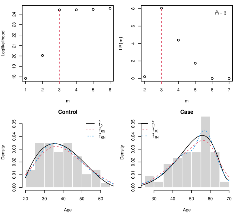
Figure 1: Coronary Heart Disease Data. Upper left panel: log-likelihood of the data; upper right panel: likelihood ratio for change-point estimate. Lower panel: histograms(light gray), the MABLE $\hat{f}_{i}$, the semparametric kernel density estimate $\tilde{f}_{i\mathrm{S}}$, and the one-sample nonparametric kernel density estimate $\tilde{f}_{i\mathrm{N}}$ of $f_{i}$, $i=0,1$.

3.2 Pancreatic Cancer Data

We apply the proposed method to the Pancreatic cancer diagnostic marker data in which sera from $n_{0}=51$ control patients with pancreatitis and $n_{1}=90$ case patients with pancreatic cancer were studied at the Mayo Clinic with a cancer antigen, CA-125, and with a carbohydrate antigen, CA19-9. Wieand et al. (1989) showed that CA19-9 has higher sensitivity to Pancreatic cancer. Let $y_{ij}$, $j=1,\ldots,n_{i}$, $i=0,1$, denote the logarithm of the observed value of CA19-9 for the $j$th subject of control group ($i=0$) and case group ($i=1$). The combined sample is $\{z_{1},\ldots,z_{n}\}$, $n=n_{0}+n_{1}$. Qin and Zhang (2003) considered the measurement $y$ on CA19-9 and obtained $p$-value 0.769 of the Kolmogorov–Smirnov–test for the density ratio model with $r(y)=(y,y^{2})^{\mathrm{\scriptscriptstyle\top}}$. Qin and Zhang (2003)’s MELE is $\tilde{\bm{\alpha}}=(0.56,-1.91,0.45)^{\mathrm{\scriptscriptstyle\top}}$ with SE $(1.66,1.22,0.21)^{\mathrm{\scriptscriptstyle\top}}$.

We choose $a=z_{(1)}=0.8754687$ and $b=z_{(n)}=10.08581$. The estimated lower bounds for $m$ based on “control” and “case” data are, respectively, $\hat{m}_{b}^{(0)}=19$ and $\hat{m}_{b}^{(1)}=2$. We chose “case” as baseline. Based on the transformed data $x_{ij}=(y_{ij}-a)/(b-a)$, we obtain an optimal degree $\tilde{m}=\hat{m}=3$ and estimates $\hat{f}_{i}$, $i=0,1$, as given by (5) with $m=3$, where $\hat{\bm{\alpha}}=(0.045,-1.677,0.434)^{\mathrm{\scriptscriptstyle\top}}$ with SE $(1.35,0.91,0.15)^{\mathrm{\scriptscriptstyle\top}}$ based 1000 bootstrap runs, and $(\hat{p}_{0},\ldots,\hat{p}_{3})=(0.09747,0.42829,0.38557,0.08867)$. The case density estimates agree each other. These results show that healthy people have lower logarithmic level of CA 19-9 in their blood while logarithmic levels of CA 19-9 for pancreatic cancer patients are nearly uniform.

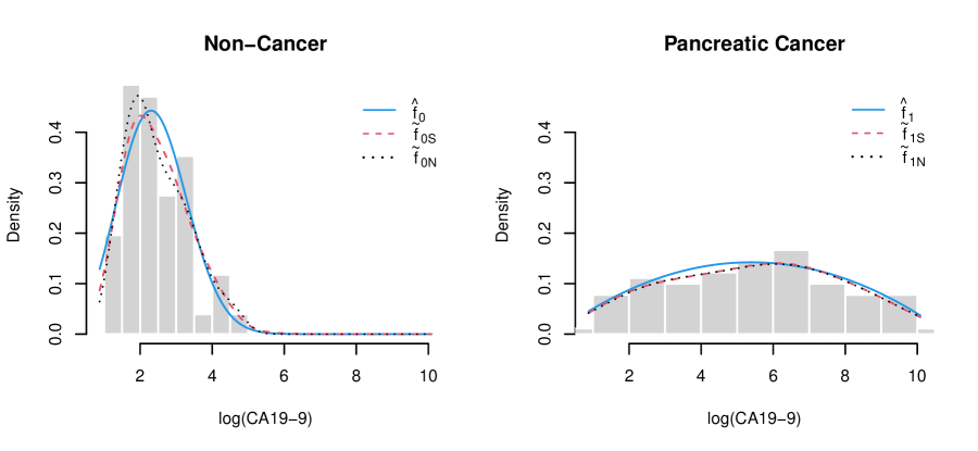
Figure 2: Pancreatic cancer CA 19-9 data. Histograms(light gray) and density estimates of log CA 19-9 level without pancreatic cancer (left panel) and with pancreatic cancer (right panel): the MABLE $\hat{f}_{i}$, the semparametric kernel density estimate $\tilde{f}_{i\mathrm{S}}$, and the one-sample nonparametric kernel density estimate $\tilde{f}_{i\mathrm{N}}$ of $f_{i}$, $i=0,1$.

3.3 Melanoma Data

Venkatraman and Begg (1996) compared two systems which can be used to evaluate suspicious lesions of being a melanoma based on paired data. The two systems are the clinical score system given by doctors and the dermoscope. Qin and Zhang (2003) suggest the density ratio model with $r(x)=x$. The MELE of $\bm{\alpha}$ is $\tilde{\bm{\alpha}}=(0.887,1.000)$ with SE $(0.37,0.23)^{\mathrm{\scriptscriptstyle\top}}$.

Using the proposed method with $a=z_{(1)}=-6.5$ and $b=5.0$ we have model degree $\hat{m}=\tilde{m}=10$. We obtained the MABLE $\hat{\bm{\alpha}}=(0.881,1.018)^{\mathrm{\scriptscriptstyle\top}}$ of $\bm{\alpha}$ with SE $(0.75,0.77)^{\mathrm{\scriptscriptstyle\top}}$ based 1000 bootstrap runs, $\hat{p}_{i}<10^{-5}$, $i\notin\mathbb{I}_{2}^{5}$, and $(\hat{p}_{2},\cdots,\hat{p}_{5})=(.30153,.14619,.55226,.00002)$. From Figure 3 we see that the clinical scores have different distributions with a small overlap for people with and without melanoma.

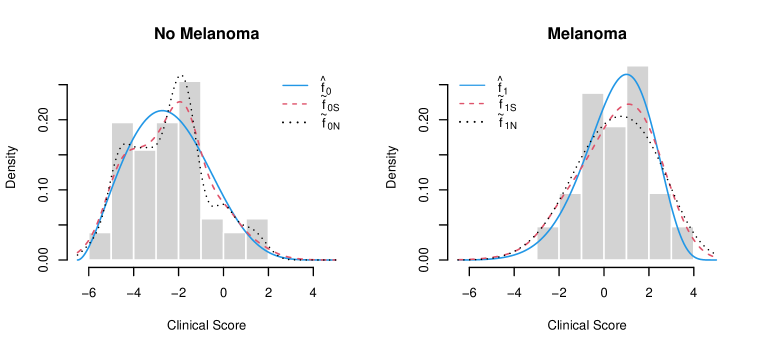
Figure 3: Melanoma data. Histograms(light gray) and density estimates of clinical scores without melanoma (left panel) and with melanoma (right panel): the MABLE $\hat{f}_{i}$, the semparametric kernel density estimate $\tilde{f}_{i\mathrm{S}}$, and the one-sample nonparametric kernel density estimate $\tilde{f}_{i\mathrm{N}}$ of $f_{i}$, $i=0,1$.

4 Simulation

In this section we compare the performances of the proposed estimator $\hat{f}_{i}$ with the one-sample parametric MLE $\hat{f}_{i\mathrm{P}}$, the two-sample semiparametric estimator $\tilde{f}_{i\mathrm{S}}$ of Qin and Zhang (2005), and the one-sample kernel density estimator $\tilde{f}_{i\mathrm{N}}$ by examining the point-wise mean squared error (pMSE) $\mathrm{mse}_{j}$ at $t_{j}=a+j(b-a)/N$, $j\in\mathbb{I}_{0}^{N}$, $N=512$) and approximate mean integrated squared error (MISE) $\mathrm{mise}=N^{-1}\sum_{j=1}^{N}\mathrm{mse}_{j}$ for $i=0,1$. For convenience and fair comparison, we used same setups as in Qin and Zhang (2005). The sample were generated using the models below. In all the simulations, the sample sizes are $(n_{0},n_{1})=(50,50),(100,100)$ and the number of Monte Carlo runs is 1000.

Model 1: Normal distributions $X_{0}\sim N(0,1)$, $X_{1}\sim N(\mu,1)$, $\tilde{r}(x)=(1,x)^{\mathrm{\scriptscriptstyle\top}}$, $f_{0}(x)=\frac{1}{\sqrt{2\pi}}e^{-x^{2}/2}$, $\bm{\alpha}=(-\mu^{2}/2,\;\mu)^{\mathrm{\scriptscriptstyle\top}}$, and $\mu=0.25(0.25)2.00$. We choose $a=\min(-4,\mu-4)$ and $b=\max(4,\mu+4)$. In this model, the bandwidths for $\tilde{f}_{i\mathrm{S}}$ and $\tilde{f}_{i\mathrm{N}}$ are those suggested by Qin and Zhang (2005). The parametric MLE is $\hat{f}_{i\mathrm{P}}(x)=f_{0}[(x-\bar{x}_{i})/s_{i}]/s_{i}$, where $\bar{x}_{i}$ and $s_{i}$ are, respectively, the sample mean and sample standard deviation of $x_{i1},\ldots,x_{in_{i}}$, $i=0,1$.

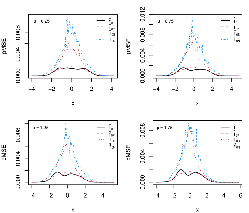
Figure 4: Simulated pointwise mean squared error of the MABLE $\hat{f}_{0}$, the one-sample parametric MLE $\hat{f}_{0\mathrm{P}}$, the semparametric kernel density estimate $\tilde{f}_{0\mathrm{S}}$, and the one-sample nonparametric kernel density estimate $\tilde{f}_{0\mathrm{N}}$ of $f_{0}$ based 1000 datasets generated from normal distributions with $n_{0}=n_{1}=50$.

Table 1: Simulation results based on $B=1000$ Monte Carlo runs and samples of sizes $(n_{0},n_{1})$ from normal distributions $\mathrm{N}(0,1)$ and $\mathrm{N}(\mu,1)$ using optimal degree $\hat{m}$.

			mse $\times 10^{2}$					mise $\times 10^{4}$
$\mu$	$E(\hat{m})$	$\sigma(\hat{m})$	$\hat{\alpha}_{0}$	$\hat{\alpha}_{1}$	$\tilde{\alpha}_{0}$	$\tilde{\alpha}_{1}$		$\hat{f}_{0\mathrm{P}}$	$\hat{f}_{0}$	$\tilde{f}_{0\mathrm{S}}$	$\tilde{f}_{0\mathrm{N}}$
	$n_{0}=n_{1}=50$
0.25	15.00	2.77	0.16	4.22	0.18	4.61		6.46	6.24	16.22	24.93
0.50	16.25	2.92	0.54	4.44	0.65	5.07		6.15	5.81	14.92	21.27
0.75	17.29	2.91	1.29	5.06	1.54	6.06		5.94	5.57	15.86	21.31
1.00	18.29	3.06	2.52	5.95	3.07	7.37		5.52	5.14	16.11	21.66
1.25	19.31	3.28	4.40	7.24	5.73	9.49		5.68	5.65	14.87	19.65
1.50	20.45	3.25	6.99	8.97	10.37	13.57		5.47	5.82	16.88	20.99
1.75	21.47	3.40	10.46	10.37	15.60	16.19		5.48	5.69	17.19	19.66
2.00	22.83	3.47	15.48	12.51	28.62	23.05		5.15	5.94	18.56	19.88
	$n_{0}=n_{1}=100$
0.25	15.20	2.16	0.07	2.23	0.08	2.32		3.05	3.52	8.76	12.56
0.50	16.28	2.49	0.28	2.33	0.30	2.53		3.09	3.55	8.18	11.87
0.75	17.27	2.33	0.65	2.61	0.72	2.77		2.84	3.26	8.49	12.26
1.00	18.42	2.58	1.20	3.03	1.32	3.37		2.74	3.17	9.30	12.26
1.25	19.51	2.60	2.08	3.37	2.34	3.84		2.78	3.11	9.56	12.12
1.50	20.60	2.75	3.69	4.49	4.52	5.62		2.64	2.83	9.22	11.56
1.75	21.61	2.80	5.47	5.32	6.73	6.60		2.54	2.93	9.67	11.29
2.00	23.02	2.94	8.17	6.02	11.15	8.32		2.45	3.01	10.09	11.61

Model 2: Exponential distributions $X_{0}$ is exponential with density $f_{0}(x)=e^{-x}$, $x>0$. $X_{1}$ is exponential with density $f_{1}(x)=\mu^{-1}e^{-x/\mu}=f_{0}(x)e^{-\log\mu+(1-1/\mu)x}$, $x>0$, where $\mu=1.25(0.25)3.00$ as in Qin and Zhang (2005). We choose $a=0$, $b=5\mu$, In this model, the bandwidths for $\tilde{f}_{i\mathrm{S}}$ and $\tilde{f}_{i\mathrm{N}}$ in Table 2 are those suggested by Qin and Zhang (2005). The parametric MLE is $\hat{f}_{i\mathrm{P}}(x)=f_{0}(x/\bar{x}_{i})/\bar{x}_{i}$, where $\bar{x}_{i}$ is the sample mean of $x_{i1},\ldots,x_{in_{i}}$, $i=0,1$.

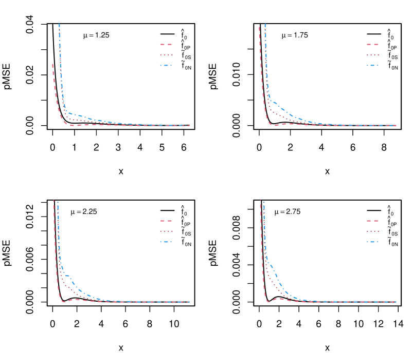
Figure 5: Simulated pointwise mean squared error of the MABLE $\hat{f}_{0}$, the one-sample parametric MLE $\hat{f}_{0\mathrm{P}}$, the semparametric kernel density estimate $\tilde{f}_{0\mathrm{S}}$, and the one-sample nonparametric kernel density estimate $\tilde{f}_{0\mathrm{N}}$ of $f_{0}$ based on 1000 datasets generated from exponential distributions with $n_{0}=n_{1}=50$.

Table 2: Simulation results based on $B=1000$ Monte Carlo runs and samples of sizes $(n_{0},n_{1})$ from exponential distributions $\mathrm{Exp}(1)$ and $\mathrm{Exp}(\mu)$ using optimal degree $m=\tilde{m}$.

			mse $\times 10^{2}$					mise $\times 10^{4}$
$\mu$	$E(\tilde{m})$	$\sigma(\tilde{m})$	$\hat{\alpha}_{0}$	$\hat{\alpha}_{1}$	$\tilde{\alpha}_{0}$	$\tilde{\alpha}_{1}$		$\hat{f}_{0\mathrm{P}}$	$\hat{f}_{0}$	$\tilde{f}_{0\mathrm{S}}$	$\tilde{f}_{0\mathrm{N}}$
	$n_{0}=n_{1}=50$
1.25	5.04	2.45	5.01	4.46	4.93	4.41		8.39	11.61	91.98	99.95
1.50	4.87	1.96	5.07	4.01	5.29	4.10		7.00	8.54	75.84	82.96
1.75	4.72	1.81	4.94	3.42	5.81	3.79		5.59	6.69	66.23	72.76
2.00	4.68	2.25	5.03	3.53	6.33	4.06		5.82	6.75	58.51	63.84
2.25	4.70	2.54	4.64	3.06	6.46	3.75		4.82	5.45	52.16	56.51
2.50	4.66	2.81	4.71	3.20	7.46	4.16		4.42	4.89	48.76	53.04
2.75	4.54	2.20	4.54	3.13	7.28	3.99		4.21	4.59	44.03	47.72
3.00	4.58	2.87	5.25	2.96	8.99	4.14		3.39	3.68	40.62	43.90
	$n_{0}=n_{1}=100$
1.25	4.61	1.12	2.60	2.26	2.47	2.15		4.19	5.99	62.32	90.99
1.50	4.46	1.05	2.32	1.87	2.48	1.88		3.62	4.55	58.10	80.45
1.75	4.33	0.83	2.29	1.67	2.66	1.79		2.92	3.62	49.12	65.99
2.00	4.22	0.75	2.36	1.66	3.00	1.86		2.73	3.09	44.31	58.99
2.25	4.18	0.69	2.01	1.41	2.94	1.69		2.31	2.62	41.40	52.25
2.50	4.15	0.37	2.40	1.64	3.50	1.95		2.34	2.44	38.76	48.49
2.75	4.18	0.56	2.09	1.32	3.27	1.66		1.86	1.98	34.80	41.90
3.00	4.22	0.76	2.45	1.53	4.01	2.03		1.97	2.05	33.19	40.12

The kernel density estimates suffers from serious boundary effect for a densities like expontial distribution. In the simulation presented in Figure 5 both $\tilde{f}_{i\mathrm{N}}$ and $\tilde{f}_{i\mathrm{S}}$ used the same bandwidth selected by the default method of R function “density()” which seems a little better than those selected by the method of Qin and Zhang (2005).

From the above simulation results we observe the folloowing. (i) The optimal degree increases slowly as sample sizes increase; (ii) As sample sizes increase the variation of the optimal degree decreases; (iii) The larger $\alpha_{1}$ is the more eficient the proposed estimator $\hat{\alpha}_{1}$ is than $\tilde{\alpha}_{1}$; (iv) The proposed estimator $\hat{f}_{0}$ is very similar to the parametric one but is much better than the semiparamtric and the nonparametric ones.

5 Large Sample Properties

We denote the chi-squared divergence($\chi^{2}$-distance) between densities $\varphi$ and $\psi$ by

$$\chi^{2}(\varphi\|\psi)=\int_{-\infty}^{\infty}\frac{[\varphi(y)-\psi(y)]^{2}}{\psi(y)}dy\equiv\int_{-\infty}^{\infty}\Big{[}\frac{\varphi}{\psi}(y)-1\Big{]}^{2}\psi(y)dy.$$

We need the following assumptions for the asymptotic properties of $\hat{f}_{\mathrm{B}}$ which will be proved in the appendix:

(A.1).

There exists $\bm{p}_{0}\in\mathbb{S}_{m}$ and $k>0$ such that $[{f_{m}(x;\bm{p}_{0})-f_{0}(x)}]/{f_{0}(x)}=\mathcal{O}(m^{-k/2})$, uniformly in $x\in[0,1]$, and thus $\chi^{2}(f_{m}(\cdot;\bm{p}_{0})\|f_{0})=\mathcal{O}(m^{-k})$.

(A.2).

Assume that the zero vector $\bm{0}\in\mathcal{A}$ and that the components of $\tilde{r}(x)$ are linearly independent.

Let $C^{(r)}[0,1]$ be the class of functions which have $r$th continuous derivative $f^{(r)}$ on $[0,1]$. If $f_{0}\in C^{(r)}[0,1]$, and $f_{0}(x)\geq b_{0}>0$, $x\in[0,1]$, then Assumption (A.1) is fulfilled with $k=r$ (Lorentz, 1963).

A weaker sufficient condition can assure Assumption (A.1). A function $f$ is said to be $\gamma$–Hölder continuous with $\gamma\in(0,1]$ if $|f(x)-f(y)|\leq C|x-y|^{\gamma}$ for some constant $C>0$. The following (Lemma 3.1 of Wang and Guan, 2019) is a generalization of the result of Lorentz (1963) which requires a positive lower bound for $f_{0}$.

Lemma 1.

Suppose that $f_{0}(x)=x^{a}(1-x)^{b}\varphi_{0}(x)$ is a density on $[0,1]$, $a$ and $b$ are nonnegative real numbers, $\varphi_{0}\in C^{(r)}[0,1]$, $r\geq 0$, $\varphi_{0}(x)\geq b_{0}>0$, and $\varphi_{0}^{(r)}$ is $\gamma$-Hölder continuous with $\gamma\in(0,1]$. Then Assumption (A.1) is fulfilled with $k=r+\gamma$.

We have the following asymptotic results in terms of distances $D^{2}_{0}(\bm{\alpha},\bm{p})=\chi^{2}(f_{m}(\cdot;\bm{p})\|f_{0})$ and $D^{2}_{1}(\bm{\alpha},\bm{p})=\chi^{2}(f_{m}(\cdot;\bm{\alpha},\bm{p})\|f_{1})$.

Theorem 1.

Under the density ratio model (1) and the assumptions (A.1) with $k>0$, and (A.2), as $n\to\infty$, with probability one the maximum value of $\ell_{m}(\bm{\alpha},\bm{p})$ with $m={\cal O}(n^{1/k})$ is attained at $(\hat{\bm{\alpha}},\hat{\bm{p}})$ in the interior of $\mathbb{B}_{m}(r_{n})=\{(\bm{\alpha},\bm{p})\in\Theta_{m}(\mathcal{A})\,:\,D^{2}_{i}(\bm{\alpha},\bm{p})\leq r_{n},\,i=0,1\},$ where $r_{n}=n^{-1}\log n$. Thus the mean $\chi^{2}$-distance between $f_{m}(\cdot;i\hat{\bm{\alpha}},\hat{\bm{p}})$ and $f_{i}(\cdot)$ satisfies

$$\mathrm{E}[D^{2}_{i}(\hat{\bm{\alpha}},\hat{\bm{p}})]=\mathrm{E}\int\frac{[f_{m}(x;i\hat{\bm{\alpha}},\hat{\bm{p}}_{m})-f_{i}(x)]^{2}}{f_{i}(x)}dx=\mathcal{O}\left(\frac{\log n}{n}\right),\;i=0,1.$$ (12)

Moreover, almost surely, $\|\hat{\bm{\alpha}}-\bm{\alpha}_{0}\|^{2}=\mathcal{O}(\log n/n)$.

Remark 1.

Theorem 1 implies that $|\hat{F}_{i}(x)-F_{i}(x)|^{2}=\mathcal{O}(\log n/n)$, uniformly on $[0,1]$, a.s., $i=0,1$.

6 Concluding Remark

Unlike the empirical likelihood method of Qin and Zhang (2003, 2005) in which an estimate of a discrete probability mass function is obtained first then smoothed using kernel method, the proposed method produces smooth estimates of density and distribution functions directly. From the simulation study we also conclude that the proposed method does not only simply smooth the estimation but also gives more accurate estimates. The improvement over the existing methods is significant especially for small samples. The proposed method also gives better estimates of coefficients of logistic regression for retrospective sampling data especially for samll sample data. Although the optimal model degree is large for some data the effective degrees of freedom, the number of nonzero mixing proportions $\hat{p}_{i}$, is usually much smaller. Instead of the exponential tilting model (1), we can consider an even more general weighted model $f_{1}(x)=f_{0}(x)w(x;\bm{\alpha}),$ where $w(x;\bm{\alpha})$ is a known nonnegative weight with unknown parameter $\bm{\alpha}$ and satisfies $\int w(x;\bm{\alpha})f_{0}(x)dx=1$ and $w(x;\bm{0})=1$.

Appendix

6.1 Proof of Proposition 1

Proof.

For any $f_{m}(x;\bm{\alpha},\bm{p}_{m})\in\mathcal{D}_{m}(\mathcal{A})$, we have $f_{m}(x;\bm{p}_{m})=\sum_{j=0}^{m}p_{mj}\beta_{mj}(x),$ and

$$\sum_{i=0}^{m}p_{mi}w_{mi}(\bm{\alpha})=\int_{0}^{1}f_{m}(x;\bm{p}_{m})\exp\{\bm{\alpha}^{\mathrm{\scriptscriptstyle\top}}\tilde{r}(x)\}dx=1,$$

so that $f_{m}(x;\bm{\alpha},\bm{p}_{m})=f_{m}(x;\bm{p}_{m})\exp\{\bm{\alpha}^{\mathrm{\scriptscriptstyle\top}}\tilde{r}(x)\}$. By Property 3.1. of Wang and Ghosh (2012) or Lemma 2.2 of Guan (2017) we also have that $f_{m}(x;\bm{p}_{m})=f_{m+1}(x;\bm{p}_{m+1})=\sum_{j=0}^{m+1}p_{m+1,j}\beta_{m+1,j}(x)$ with $p_{m+1,0}=(m+1)p_{m0}/(m+2)$, $p_{m+1,m+1}=(m+1)p_{mm}/(m+2)$, and $p_{m+1,j}=\left[{j}p_{m,j-1}+{(m-j+1)}p_{mj}\right]/({m+2})$, $j\in\mathbb{I}_{1}^{m}.$ Thus we have $f_{m}(x;\bm{\alpha},\bm{p}_{m})=f_{m+1}(x;\bm{p}_{m+1})\exp\{\bm{\alpha}^{\mathrm{\scriptscriptstyle\top}}\tilde{r}(x)\}=f_{m+1}(x;\bm{\alpha},\bm{p}_{m+1})$ and $\sum_{i=0}^{m+1}p_{m+1,i}w_{m+1,i}(\bm{\alpha})=1$. Hence $f_{m}(x;\bm{\alpha},\bm{p}_{m})\in\mathcal{D}_{m+1}(\mathcal{A})$. ∎

6.2 Proof of Theorem 1

Proof.

Let $\bm{\alpha}_{0}=(\alpha_{00},\ldots,\alpha_{0d})^{\mathrm{\scriptscriptstyle\top}}$ be the true value of $\bm{\alpha}$ so that $\int_{0}^{1}f_{0}(x)\exp\{\bm{\alpha}_{0}^{\mathrm{\scriptscriptstyle\top}}\tilde{r}(x)\}dx=1.$ By Assumption (A.1), we have

$$f_{m}(x;i\bm{\alpha}_{0},\bm{p}_{0})=f_{i}(x)+R_{m}(x)\exp\{i\bm{\alpha}_{0}^{\mathrm{\scriptscriptstyle\top}}\tilde{r}(x)\},\quad i=0,1,$$ (13)

where $R_{m}(x)=f_{0}(x)\mathcal{O}(m^{-r/2})$. Thus $\int_{0}^{1}f_{m}(x;\bm{\alpha}_{0},\bm{p}_{0})dx=1+\int_{0}^{1}R_{m}(x)\exp\{i\bm{\alpha}_{0}^{\mathrm{\scriptscriptstyle\top}}\tilde{r}(x)\}dx=1+\rho_{m},$ where $\rho_{m}=\mathcal{O}(m^{-r/2})$. If we define $\tilde{\bm{\alpha}}_{0}=\tilde{\bm{\alpha}}_{0}{(m)}=(\tilde{\alpha}_{00},\alpha_{01},\ldots,\alpha_{0d})^{\mathrm{\scriptscriptstyle\top}}$ with $\tilde{\alpha}_{00}=\alpha_{00}-\log(1+\rho_{m})$, then we have $|\tilde{\bm{\alpha}}_{0}{(m)}-\bm{\alpha}_{0}|=|\log(1+\rho_{m})|=\mathcal{O}(m^{-r/2})$, $\int_{0}^{1}f_{m}(x;\tilde{\bm{\alpha}}_{0},\bm{p}_{0})dx=\sum_{j=0}^{m}p_{0j}w_{mj}(\tilde{\bm{\alpha}}_{0})=1$, and

$$\frac{f_{m}(x;\tilde{\bm{\alpha}}_{0},\bm{p}_{0})-f_{1}(x)}{f_{1}(x)}=\frac{R_{m}(x)}{(1+\rho_{m})f_{0}(x)}-\frac{\rho_{m}}{1+\rho_{m}}=\mathcal{O}(m^{-r/2}).$$

Define the log-likelihood ratio $\mathcal{R}(\bm{\alpha},\bm{p})=\ell(\bm{\alpha}_{0},f_{0})-\ell_{m}(\bm{\alpha},\bm{p})$. Thus we have

$$\mathcal{R}(\bm{\alpha},\bm{p}) = -\sum_{i=0}^{1}\sum_{j=1}^{n_{i}}\log[f_{m}(x_{ij};i\bm{\alpha},\bm{p})/f_{i}(x_{ij})].$$ (14)

Consider subsets

$$\Theta(\epsilon_{0})=\{(\bm{\alpha},\bm{p})\in\Theta_{m}(\mathcal{A}):\mbox{$\forall$ $x\in[0,1]$, $i=0,1$, $|f_{m}(x;i\bm{\alpha},\bm{p})/f_{i}(x)-1|\leq\epsilon_{0}$}\},$$

$0<\epsilon_{0}<1$. Clearly, by (A.1) and (13), $\Theta(\epsilon_{0})$ is nonempty if $m$ is large enough.

By Taylor expansion we have, for $(\bm{\alpha},\bm{p})\in\Theta(\epsilon_{0})$, $0<\epsilon_{0}<1$, and large $m$,

$$\mathcal{R}(\bm{\alpha},\bm{p}) = \sum_{i=0}^{1}\left\{\sum_{j=1}^{n_{i}}\Big{[}\frac{1}{2}U_{ij}^{2}(\bm{\alpha},\bm{p})-U_{ij}(\bm{\alpha},\bm{p})\Big{]}+\mathcal{O}(R_{mi}(\bm{\alpha},\bm{p}))\right\},\,a.s.,$$

where $U_{ij}(\bm{\alpha},\bm{p})=[{f_{m}(x_{ij};i\bm{\alpha},\bm{p})-f_{i}(x_{ij})}]/{f_{i}(x_{ij})}$, $j\in\mathbb{I}_{1}^{n_{i}}$, and $R_{mi}(\bm{\alpha},\bm{p})=\sum_{j=1}^{n_{i}}U_{ij}^{2}(\bm{\alpha},\bm{p})$, $i=0,1.$ Since $\mathrm{E}[U_{ij}(\bm{\alpha},\bm{p})]=0$, $\sigma^{2}[U_{ij}(\bm{\alpha},\bm{p})]=\mathrm{E}[U_{ij}^{2}(\bm{\alpha},\bm{p})]=D^{2}_{i}(\bm{\alpha},\bm{p})$, by the LIL we have $\sum_{j=1}^{n}U_{ij}(\bm{\alpha},\bm{p})/\sigma[U_{ij}(\bm{\alpha},\bm{p})]=\mathcal{O}(\sqrt{n\log\log n})$, a.s.. By the strong law of large numbers we have, a.s.,

$$\mathcal{R}(\bm{\alpha},\bm{p})=\sum_{i=0}^{1}\left\{\frac{n}{2}D^{2}_{i}(\bm{\alpha},\bm{p})-\mathcal{O}(D_{i}(\bm{\alpha},\bm{p})\sqrt{n\log\log n})+o(nD^{2}_{i}(\bm{\alpha},\bm{p}))\right\}.$$ (15)

If $D^{2}_{i}(\bm{\alpha},\bm{p})=r_{n}=\log n/n$, then, by (15), there is an $\eta>0$ such that $\mathcal{R}(\bm{\alpha},\bm{p})\geq\eta\log n,\,a.s..$ If $(\bm{\alpha},\bm{p})=(\tilde{\bm{\alpha}}_{0},\bm{p}_{0})$ and $m=Cn^{1/k}$, we have $D^{2}_{i}(\tilde{\bm{\alpha}}_{0},\bm{p}_{0})=\mathcal{O}(m^{-k})=\mathcal{O}(n^{-1})$. By (15) again we have $\mathcal{R}(\tilde{\bm{\alpha}}_{0},\bm{p}_{0})=\mathcal{O}(\sqrt{\log\log n})$, a.s.. Therefore, similar to the proof of Lemma 1 of Qin and Lawless (1994), we have

$$D^{2}_{i}(\hat{\bm{\alpha}},\hat{\bm{p}})=\int_{0}^{1}\frac{[f_{m}(x;i\hat{\bm{\alpha}},\hat{\bm{p}})-f_{i}(x)]^{2}}{f_{i}(x)}dx\leq\frac{\log n}{n},a.s.,$$ (16)

and $(\hat{\bm{\alpha}},\hat{\bm{p}})\in\Theta(\epsilon_{0})$. Thus (12) follows. Define

$$\psi({\bm{\alpha}},g)=\int_{0}^{1}\frac{g^{2}(x;{\bm{p}})}{f_{0}^{2}(x)}\left[\frac{w(x;{\bm{\alpha}})}{w(x;{\bm{\alpha}}_{0})}-1\right]^{2}f_{1}(x)dx,$$

where $w(x;{\bm{\alpha}})=\exp\{\bm{\alpha}^{\mathrm{\scriptscriptstyle\top}}\tilde{r}(x)\}$ and $g$ is a density on $[0,1]$. Then we have

$$\psi(\hat{\bm{\alpha}},\hat{f}_{0}) \leq 2D^{2}_{1}(\hat{\bm{\alpha}},\hat{\bm{p}})+2\int_{0}^{1}\left[\frac{f_{m}(x;\hat{\bm{p}})}{f_{0}(x)}-1\right]^{2}f_{1}(x)dx$$

$$\leq 2D^{2}_{1}(\hat{\bm{\alpha}},\hat{\bm{p}})+2CD^{2}_{0}(\hat{\bm{\alpha}},\hat{\bm{p}})$$

$$= \mathcal{O}(\log n/n),$$

where $C=\max_{x\in[0,1]}w(x;{\bm{\alpha}}_{0})$. It is clear that $\psi(\bm{\alpha}_{0},g)=0$, $\dot{\psi}(\bm{\alpha}_{0},g)=0$ and

$$\ddot{\psi}(\bm{\alpha}_{0},f_{0})=2\int_{0}^{1}\tilde{r}(x)\tilde{r}^{\mathrm{\scriptscriptstyle\top}}(x)f_{1}(x)dx\equiv 2J(\bm{\alpha}_{0}).$$

By Taylor expansion and (16) we have $\psi(\hat{\bm{\alpha}},\hat{f}_{m})=(\hat{\bm{\alpha}}-\bm{\alpha}_{0})^{\mathrm{\scriptscriptstyle\top}}J(\bm{\alpha}_{0})(\hat{\bm{\alpha}}-\bm{\alpha}_{0})+o(R_{n}),$ where $R_{n}=\|\hat{\bm{\alpha}}-\bm{\alpha}_{0}\|^{2}+\mathcal{O}(\log n/n).$ Then we have $(\hat{\bm{\alpha}}-\bm{\alpha}_{0})^{\mathrm{\scriptscriptstyle\top}}J(\hat{\bm{\alpha}}-\bm{\alpha}_{0})+o(\|\hat{\bm{\alpha}}-\bm{\alpha}_{0}\|^{2})=\psi(\hat{\bm{\alpha}},\hat{f}_{m})+o(\log n/n)$ and thus $(\lambda_{0}+o(1))\|\hat{\bm{\alpha}}-\bm{\alpha}_{0}\|^{2}\leq\mathcal{O}(\log n/n)$, where $\lambda_{0}$ is the minimum eigenvalue of $J(\bm{\alpha}_{0})$. Because the components of $\tilde{r}(x)=(1,r^{\mathrm{\scriptscriptstyle\top}}(x))^{\mathrm{\scriptscriptstyle\top}}$ are linearly independent, $J(\bm{\alpha}_{0})$ is positive definite. Thus $\lambda_{0}>0$ and we have $\|\hat{\bm{\alpha}}-\bm{\alpha}_{0}\|^{2}=\mathcal{O}(\log n/n)$, a.s.. The proof is complete. ∎

References

- Bickel et al. (1993) Bickel, P. J., Klaassen, C. A. J., Ritov, Y., and Wellner, J. A. (1993), Efficient and adaptive estimation for semiparametric models, Johns Hopkins Series in the Mathematical Sciences, Johns Hopkins University Press, Baltimore, MD.
- Cheng and Chu (2004) Cheng, K. F., and Chu, C. K. (2004), “Semiparametric density estimation under a two-sample density ratio model,” Bernoulli, 10, 583–604.
- Cox (1972) Cox, D. R. (1972), “Regression models and life-tables,” J. Roy. Statist. Soc. Ser. B, 34, 187–220.
- Dabrowska and Doksum (1988) Dabrowska, D. M., and Doksum, K. A. (1988), “Estimation and testing in a two-sample generalized odds-rate model,” J. Amer. Statist. Assoc., 83, 744–749.
- Efron and Tibshirani (1996) Efron, B., and Tibshirani, R. (1996), “Using specially designed exponential families for density estimation,” Annals of Statistics, 24, 2431–2461.
- Guan (2016) Guan, Z. (2016), “Efficient and robust density estimation using Bernstein type polynomials,” Journal of Nonparametric Statistics, 28, 250–271.
- Guan (2017) — (2017), “Bernstein Polynomial Model for Grouped Continuous Data,” Journal of Nonparametric Statistics, 29, 831–848.
- Guan (2019) — (2019), mable: Maximum Approximate Bernstein/Beta Likelihood Estimation, r package version 3.0.
- Guan (2021a) — (2021a), “Fast Nonparametric Maximum Likelihood Density Deconvolution Using Bernstein Polynomials,” Statistica Sinica, 31, to appear.
- Guan (2021b) — (2021b), “Maximum approximate Bernstein likelihood estimation in proportional hazard model for interval-censored data,” Statistics in Medicine, 40, 758–778.