Randomization inference for composite experiments with spillovers and peer effects

Abstract

Group-formation experiments, in which experimental units are randomly assigned to groups, are a powerful tool for studying peer effects in the social sciences. Existing design and analysis approaches allow researchers to draw inference from such experiments without relying on parametric assumptions. In practice, however, group-formation experiments are often coupled with a second, external intervention, that is not accounted for by standard nonparametric approaches. This note shows how to construct Fisherian randomization tests and Neymanian asymptotic confidence intervals for such composite experiments, including in settings where the second intervention exhibits spillovers. We also propose an approach for designing optimal composite experiments.

Keywords: Causal inference; Conditional randomization test; Exact $p$-value; Non-sharp null hypothesis; Orbit-Stabilizer Theorem

1 Introduction

When studying social systems and organizations, quantitative researchers are often interested in whether the behavior of an individual is affected by the characteristics of other individuals in the system: this phenomenon is called a peer effect. A common approach for studying peer effects is the so-called group-formation experiment, whereby units are randomly split into groups. An early example is a study conducted by Sacerdote (2001), who leveraged the random assignment of roommates at Dartmouth to assess whether the drinking behavior of freshmen affected that of their roommates. In recent work, Li et al. (2019) and Basse et al. (2019) developed a framework for designing and analyzing these types of experiments in a randomization-based framework; that is, without assuming a response model for the outcomes, and relying on the random assignment as the sole basis for inference.

However, group-formation experiments are often coupled with an additional intervention to form what we call a composite experiment: typically, units would first be split into groups, then a treatment would be randomized to a subset of the individuals in the experimental population. For instance, in their study of peer-effects in the context of the spread of managerial best practices, Cai and Szeidl (2018) randomized the managers of different-sized firms into groups, then provided a random subset of the managers with special information. Similarly, in a study of student learning, Kimbrough et al. (2017) first randomized students into groups of homogeneous or heterogenous ability, then allowed a random subset of students to practice a task with other students in their group. Without the second interventions, both studies would be simple group-formation experiments, and could be analyzed with the framework of Basse et al. (2019). Similarly, if one conditions on the group composition, then the second part of the composite experiment is just a classical randomized experiment, and the effects of interest fit in the usual causal inference framework.

This article shows how to study jointly the peer-effects and causal effects of a composite experiment. Our key insight is that the effects of both the group-formation and the additional intervention can be summarized into an exposure, or effective treatment. In particular, this approach allows us to accomodate the fact that the second intervention may exhibit spillover effects. Building on the group theoretical framework of Basse et al. (2019), we propose a class of designs that is amenable both to inference in the Neyman model for exposure contrasts, and to conditional randomization tests that can be implemented with simple permutations of the exposures. Within that class of designs, we derive optimal designs by solving a simple integer programming problem: in some simulation settings, we found that optimal designs increase the power by 80 percentage points over valid but more naive designs.

2 Setup and framework

2.1 Composite experiments and potential outcomes framework

We consider $N$ units indexed by $i=1,\ldots,N$, each with a fixed attribute $A_{i}\in\mathcal{A}$, which are assigned to two successive interventions. In the first intervention, the group-formation intervention, the $N=m\times K$ units are randomly assigned to $K$ distinct groups of equal size $m$. Following Basse et al. (2019), we denote by $L_{i}\in\{1,\ldots,K\}$ the group to which unit $i$ is assigned, and denote by $L=(L_{1},\ldots,L_{N})$ the group assignment vector. For each group assignment vector $L$, define the neighbor assignment vector $Z(L)=(Z_{1}(L),\ldots,Z_{N}(L))$, where $Z_{i}(L)=\{j\in\mathbb{I}\setminus\{i\}:L_{i}=L_{j}\},\forall i\in\mathbb{I}.$ To simplify the notation, the dependence of $Z$ on $L$ will often be omitted. In the second intervention, the treatment intervention, units are randomly assigned to a treatment, with $W_{i}\in\mathcal{W}$ being a treatment indicator for unit $i$ and $W=(W_{1},\ldots,W_{N})$ the treatment assignment vector. We denote by $Y_{i}(Z,W)$ the potential outcome of unit $i$ which, a priori, may depend on the entire group assignment vector $Z$ and treament assignment vector $W$. Throughout, we will adopt the randomization-based perspective, considering the potential outcomes as fixed quantities, the randomness coming exclusively from $Z$ and $W$. Basse et al. (2019) studied the group-formation intervention, with no treatment intervention. In contrast, the bulk of the literature on interference in causal inference focuses on treatment interventions, without group-formation. Our setting combines both, as summarized in the left panel of Figure 1, and allows us to address a broader type of questions, as illustrated in the following examples.

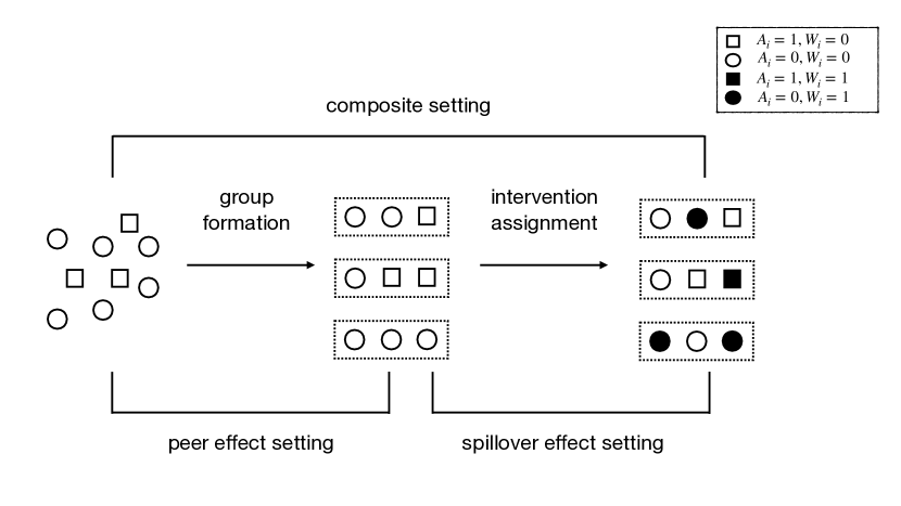
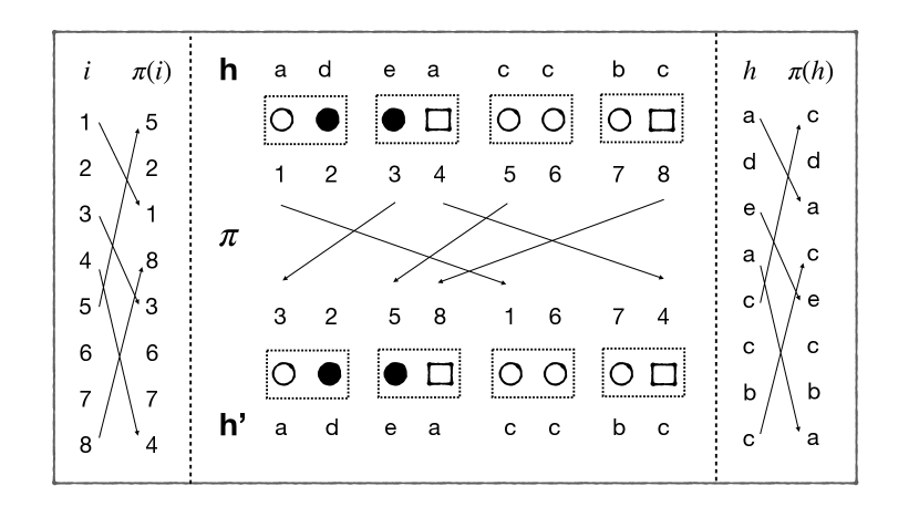
Figure 1: Left panel summarizes our composite experiment setting. Right panel illustrates our randomization procedure, as described in Definition 2.

Example 1: In the managerial setting of Cai and Szeidl (2018) described in the introduction, the attribute set $\mathcal{A}$ contains all the combinations of size and sector for the firms, and $W_{i}$ is an indicator for whether the manager of firm $i$ received special financial information.

Example 2: In the educational context of Kimbrough et al. (2017) we mentioned earlier, the attribute set $\mathcal{A}$ contains the different levels of student ability, and $W_{i}$ is an indictor for whether student $i$ was allowed to practice a task with another student.

2.2 Exposure

The potential outcomes notation $Y_{i}(Z,W)$ highlights the fact that the outcome of unit $i$ may depend on the group membership of all units, $Z$, as well as the treatment assigned to all units, $W$. In practice, it is often reasonable to assume that the outcome of unit $i$ only depends on the treatments and attributes of the units in the same group as unit $i$; that is, the outcome of unit $i$ depends on $Z$ and $W$ only through the function $h_{i}(Z,W)$ defined as:

$$h_{i}(Z,W)=(\Gamma_{i},W_{i})$$ (1)

where $\Gamma_{i}=\{(A_{j},W_{j}):j\in Z_{i}\}$. In the pure group-formation intervention, as well as in the pure treatment intervention settings, a collection of functions $h_{i}$ summarizing $Z$ or $W$ is called an exposure mapping: we will adopt this terminology as well. The local dependence captured by the specification of (1) generalizes the concept of partial interference which, in our context, can be formulated as follows:

Assumption 1.

Let $\{h_{i}\}$ be as in (1). For all $i=1,\ldots,N$, the following holds:

$$\forall(Z,W),(Z^{\prime},W^{\prime}),\qquad h_{i}(Z,W)=h_{i}(Z^{\prime},W^{\prime})\quad\Rightarrow\quad Y_{i}(Z,W)=Y_{i}(Z^{\prime},W^{\prime}).$$

With a slight abuse of notation, we will write $Y_{i}(Z,W)=Y_{i}(\Gamma_{i},W_{i})$.

If we think of the pair $(Z,W)$ as the intervention, the exposure $H_{i}=(\Gamma_{i},W_{i})$ can be thought of as the effective intervention, since it captures the part of $(Z,W)$ that actually affects the outcome of unit $i$. When both the attribute set $\mathcal{A}$ and treatment set $\mathcal{W}$ are binary, the exposure of (1) simplifies to:

$$h_{i}(Z,W)=(\Gamma_{i},W_{i})=(\sum_{j\in Z_{i}}A_{j},\sum_{j\in Z_{i}}Z_{j},\sum_{j\in Z_{i}}A_{j}W_{j},W_{i})$$ (2)

so the exposure $H_{i}$ can be summarized by a simple quadruple of values.

In practice, further restrictions of the exposure may be considered. For instance, one may assume that the interaction term $\sum_{j\in Z_{i}}A_{j}W_{j}$ does not affect the outcome, and can be removed from the exposure. While our results are derived for the more general exposure, they can be shown to hold for this simplified exposure as well.

2.3 Causal estimands and null hypotheses

We will consider two types of inferential targets, requiring two different approaches to inference. First we will consider causal estimands defined as average contrasts between different exposures. Specifically, for $\{h_{i}\}_{i=1}^{n}$ defined as in (1), let $\mathcal{H}$ be the set of all values that the exposures can take; since $H_{i}=(\Gamma_{i},W_{i})$, each element $k\in\mathcal{H}$ will be of the form $k=(\gamma,w)$. We consider the average exposure contrast between $k,k^{\prime}\in\mathcal{H}$, defined as $\tau(k,k^{\prime})=N^{-1}\sum_{i=1}^{N}\{Y_{i}(k)-Y_{i}(k^{\prime})\}$, as well as the attribute-specific counterpart defined as $\tau_{[a]}(k,k^{\prime})=N_{[a]}^{-1}\sum_{i:A_{i}=a}\{Y_{i}(k)-Y_{i}(k^{\prime})\}$, where $N_{[a]}$ is the number of units with attribute $A_{i}=a$. Two special cases of these estimands deserve a brief mention. If $k=(\gamma,w)$ and $k^{\prime}=(\gamma^{\prime},w^{\prime})$ are such that $w=w^{\prime}$, then the estimand focuses on the effect of peer’s attributes and treatments. If $k$ and $k^{\prime}$ are such that $\gamma^{\prime}=\gamma$, then the estimand focuses on the effect of each unit’s treatment, for fixed levels of peer attributes and peer treatments. Second, we will consider two types of null hypotheses. The global null hypothesis

$$H_{0}:Y_{i}(\gamma_{1},w_{1})=Y_{i}(\gamma_{2},w_{2}),\forall(\gamma_{1},w_{1}),(\gamma_{2},w_{2})\in\mathcal{H},\forall i\in\mathbb{I}$$

asserts that the combined intervention has no effect whatsoever on any unit. Of more practical interest are pairwise null hypotheses of the form

$$H_{0}^{(\gamma_{1},w_{1}),(\gamma_{2},w_{2})}:Y_{i}(\gamma_{1},w_{1})=Y_{i}(\gamma_{2},w_{2}),\forall i\in\mathbb{I}.$$

The global null hypothesis can be easily tested with a standard Fisher Randomization Test so we discuss it only in the Supplementary Material. We will focus instead on pairwise null hypotheses, which are more difficult to test since they are not sharp; that is, under the pairwise null, the observed outcomes do not determine all the potential outcomes.

2.4 Assignment mechanism and challenges

In section 2.1, we stated that both the group assignment $L$ and the treatment $W$ were assigned at random, but so far we have not discussed their distribution $\textup{pr}(L,W)$. In a randomization-based framework, this distribution is the sole basis for inference, and must be specified with care.

Building on an insight from Basse et al. (2019), notice that if we assume that the outcome of unit $i$ depends on $Z$ and $W$ only through the exposure $H_{i}=h_{i}(Z(L),W)$, the problem reduces to a multi-arm trial on the exposure scale. In particular, instead of $\textup{pr}(L,W)$, one should focus on $\textup{pr}(H)$, the distribution of the exposure induced by $\textup{pr}(L,W)$. If the distribution of $\textup{pr}(H)$ is simple, estimating exposure contrasts and testing pairwise null hypotheses is straightforward. Unfortunately, the experimenter can manipulate $\textup{pr}(H)$ only indirectly, via $\textup{pr}(L,W)$. The key objective of this paper is to construct a class of designs $\textup{pr}(L,W)$ that induce simple exposure distributions $\textup{pr}(H)$; specifically, we focus on designs for which the exposure has a Stratified Completely Randomized Design.

Definition 1.

Without loss of generality, denote by $\mathcal{H}$ the set of possible exposures and $A$ an N-vector. Let $\mathbf{n}_{A}=(n_{a,h})_{a\in\mathcal{A},h\in\mathcal{H}}$, such that $\sum_{h\in\mathcal{H}}n_{a,h}=N_{[a]}$, denote a vector of non-negative integers corresponding to number of units with each possible attribute and exposure combination. We say that a distribution of exposures $\textup{pr}(H)$ is a stratified completely randomized design denoted by $\operatorname{SCRD}(\mathbf{n}_{A})$ if the following two conditions are satisfied.

1. After stratifying based on $A$, the exposure $H=(H_{1},\ldots,H_{N})$ is completely randomized. That is, (1) $\mathbb{P}(H_{i}=h)=\mathbb{P}(H_{j}=h)$ for all $h\in\mathcal{H}$ and $i,j\in\mathbb{I}$ such that $A_{i}=A_{j}$; (2) the number of units with exposure $h\in\mathcal{H}$ and stratum $a\in\mathcal{A}$ is $n_{a,h}$.

2. The exposure assignments across strata are independent. That is $\mathbb{P}(H_{i}=h_{i}|H_{j}=h_{j})=\mathbb{P}(H_{i}=h_{i})$ for all $h_{i},h_{j}\in\mathcal{H}$ and $i,j\in\mathbb{I}$ such that $A_{i}\neq A_{j}$.

This design is simple for two reasons. First, it is easy to sample from: this makes it possible to perform suitably adapted Fisher Randomization Tests, a task that would otherwise be computationally intractable (Basse et al., 2019). Second, it makes it possible to obtain inferential results for standard estimators such as the difference in means.

3 Randomization procedure and main theorem

Our main result builds on the theory developed by Basse et al. (2019), and can be summarized in one sentence: if the design $\textup{pr}(L,W)$ has certain symmetry properties, so will the exposure distribution $\textup{pr}(H)$. The right notion of symmetry can be formulated using elementary concepts from algebraic group theory.

Recall that a permutation of $\mathbb{I}=\{1,\ldots,N\}$ can be represented as a one-to-one mapping from $\mathbb{I}$ to $\mathbb{I}$. The symmetric group $S$ is the set of all permutations of $\mathbb{I}$. Let $C_{i}=(L_{i},W_{i})$ and $C=(C_{1},\ldots,C_{N})\in\mathbb{C}$. If $\pi\in S$, we denote by $\pi\cdot C=(C_{\pi^{-1}(i)})_{i=1}^{N}=(L_{\pi^{-1}(i)},W_{\pi^{-1}(i)})_{i=1}^{N}$ the operation of permuting the elements of $C$. This mathematical operation called a group action is defined more formally in the Supplement. Finally, if $C\in\mathbb{C}$, and $\Pi\subseteq S$ is a subgroup of $S$, we define the stabilizer group of $C$ in $\Pi$ as $\Pi_{C}=\{\pi\in\Pi\,:\,\pi\cdot C=C\}$. We can now introduce our proposed procedure:

Definition 2.

Given an observed attribute vector $A=(A_{1},\ldots,A_{N})$, consider the following randomization procedure.

1. Initialize $C_{0}=(W_{0}$, $L_{0})\in\mathbb{C}$.

2. Permute $C=\pi\cdot C_{0}$, where $\pi\sim\operatorname{Unif}(S_{A})$

Given a choice of $C_{0}=(W_{0},L_{0})$ this procedure yields a design $\textup{pr}(L,W)$ with two important properties. First, it is easy to sample from: drawing random permutations from $S_{A}$ and applying them to a vector $C_{0}$ can be done in just three lines of efficient $R$ code, without requiring additional packages (Basse et al., 2019). Second, it induces a simple exposure distribution, as formalized by Theorem 1 below. The choice of $C_{0}$ is important in practice, and is discussed in details in Section 5.

Theorem 1.

If $\textup{pr}(C)$ is generated from the randomization procedure in Definition 2, then the induced distribution of exposure $\textup{pr}(H)$ is $SCRD(\mathbf{n}_{A})$.

This result underpins the inferential approaches we describe in Section 4. If the treatment intervention vector $W_{0}$ is degenerate, i.e it is a vector of $0$ values, then permuting $C_{0}$ is equivalent to permuting $L_{0}$ only and Theorem 1 reduces to Theorem 1 in Basse et al. (2019).

4 Inference

4.1 Estimating the average exposure contrast

Under Assumption 1, our combined experiment can be thought of as a multi-arm trials on the exposure scale. If the groups $L$ and treatment $W$ are assigned according to Definition 2, then Theorem 1 states that this multi-arm trial follows a completely randomized design, stratified on the attribute $A$. Estimation and inference for average exposure contrast therefore follows immediately from standard results in the randomization-based inference literature Li and Ding (2017). For any $a\in\mathcal{A}$, and $k\in\mathcal{H}$, define

$$\hat{Y}_{[a]}(k)=\frac{1}{n_{[a](k)}}\sum_{i:A_{i}=a,H_{i}=k}Y_{i},$$

the average outcome for units with attribute $A_{i}=a$ who receive the exposure $H_{i}=k$, where $n_{[a]}(k)=|\{i\in\mathbb{I}:A_{i}=a,H_{i}=k\}|$. Consider $\hat{\tau}_{[a]}(k,k^{\prime})=\hat{Y}_{[a]}(k)-\hat{Y}_{[a]}(k^{\prime})$ the difference-in-means estimator within stratum $a$, and the stratified estimator $\hat{\tau}(k,k^{\prime})=\sum_{a\in\mathcal{A}}(n_{[a]}/n)\hat{\tau}_{[a]}(k,k^{\prime})$. Theorem 2 summarizes their well-studied properties (see also Theorem 3 of Li et al. (2019)).

Theorem 2.

Under the randomization procedure in 2, and standard regularity conditions, then for any $a\in\mathcal{A}$, $k,k^{\prime}\in\mathcal{H}$, the estimators $\hat{\tau}_{[a]}(k,k^{\prime})$ and $\hat{\tau}(k,k^{\prime})$ are unbiased for $\tau_{[a]}(k,k^{\prime})$ and $\tau(k,k^{\prime})$ respectively, and are asymptotically normally distributed. In addition, the standard Wald-type confidence interval for $\hat{\tau}_{[a]}(k,k^{\prime})$ and $\hat{\tau}(k,k^{\prime})$ are asymptotically conservative.

Stratified completely randomized designs also make it straightforward to incoporate covariates in the analysis; see the Supplementary Material for details.

4.2 Testing pairwise null hypotheses

Building on recent literature on testing under interference (Basse et al., 2019; Aronow, 2012; Athey et al., 2018), we construct a Fisher Randomization Test, conditioning on a focal set, defined as

$$\mathcal{U}=u(Z(L),W)=\{i\in\mathbb{I}:h_{i}(Z(L),W)\in\{(\gamma_{1},w_{1}),(\gamma_{2},w_{2})\}\}.$$

Let the test statistic $T$ be the difference in means between the focal units with exposure $(\gamma_{1},w_{1})$ and those with exposure $(\gamma_{2},w_{2})$. The following proposition defines a valid test of $H_{0}^{(\gamma_{1},w_{1}),(\gamma_{2},w_{2})}$.

Proposition 1.

Consider observed $N-$vectors of exposure $H^{obs}\sim\textup{pr}(H)$ and outcome $Y^{obs}=Y(H^{obs})$, resulting in focal set $\mathcal{U}^{obs}$ and test statistic $T^{obs}=T(H^{obs},Y^{obs},\mathcal{U}^{obs})$. If $H^{\prime}\sim\textup{pr}(H|\mathcal{U}^{obs})$ and $T^{\prime}=T(H^{\prime},Y^{obs},\mathcal{U}^{obs})$, then the following quantity,

$$\operatorname{pval}(H^{obs})=\textup{pr}(T^{\prime}\geq T^{obs}|\mathcal{U}^{obs})$$

is a valid p-value conditionally and marginally for $H_{0}^{(\gamma_{1},w_{1}),(\gamma_{2},w_{2})}$. That is, if $H_{0}^{(\gamma_{1},w_{1}),(\gamma_{2},w_{2})}$ is true, then for any $\mathcal{U}^{obs}$ and $\alpha\in[0,1]$, we have $\textup{pr}\{\operatorname{pval}(H^{obs})\leq\alpha|\mathcal{U}^{obs}\}\leq\alpha$.

Although it always leads to valid p-values, the test in Proposition 1 is computationally intractable for most choices of designs $pr(L,W)$. The challenge, as highlighted by Basse et al. (2019), is the step that requires sampling from the conditional distribution of $pr(H\mid\mathcal{U}^{obs})$: even in small samples, this cannot be accomplished by rejection sampling. Our key result in this section is that if the design is symmetric in the sense of Section 3, then the test in Proposition 1 can be carried efficiently:

Theorem 3.

Let $\textup{pr}(C)$ be generated from randomization procedure described in Definition 2 and $\textup{pr}(H)$ the induced exposure distribution. Define a focal set $\mathcal{U}=u(Z,W)=\{i\in\mathbb{I}:h_{i}(Z,W)\in\mathcal{H}_{u}\}$ for some $pr(W,Z)>0$ and set of exposures $\mathcal{H}_{u}\subset\mathcal{H}$. Let $U=(U_{1},\ldots,U_{N})$, where $U_{i}=\mathds{1}(i\in\mathcal{U})$. Then the conditional distribution of exposure, $pr(H|\mathcal{U})$, is $SCRD(\mathbf{n}_{A\mathcal{U}})$.

This theorem makes the test described in Proposition 1 computationally tractable by transforming a difficult task — sampling from an arbitrary conditional distribution — into a simple one — sampling from a stratified completely randomized design.

5 Optimal design heuristics

Definition 2 requires the specification of an initial pair $C_{0}=(L_{0},W_{0})$. A straightforward consequence of Theorem 1 is that the number of unit in a stratum $a$ receiving exposure $k$ is constant. Formally, let $H_{0}$ be the exposure corresponding to $C_{0}$, and $H$ be any exposure vector that may be induced by our procedure: we have $n_{[a]k}(H_{0})=n_{[a]k}(H)$, where $n_{[a]k}(H^{\prime})=|\{i\in\mathds{I}:H^{\prime}_{i}=k,A_{i}=a\}|$. If the experimenter knows ex-ante that she is interested in estimating $\tau(k,k^{\prime})$, or testing the pairwise null $H_{0}^{k,k^{\prime}}$, then a useful heuristic for maximizing power would be to select $C_{0}$ such that the associated exposure vector $H_{0}$ features many units with the desired exposures $k$ and $k^{\prime}$. Constructing such a $C_{0}$ manually is possible in very small toy examples, but it becomes impractical as the sample size increases even slightly. An alternative option would be to perform a random search on the space of possible pairs $C=(L,W)$, but it grows very fast as the number of clusters and their sizes increases; making the process computationally challenging. Instead we optimize our heuristic criterion directly.

Let $\mathcal{G}\subseteq(\mathcal{A}\times\mathcal{W})^{m}$ the set of all possible attribute-intervention compositions for a group of size $m$, so for any $G\in\mathcal{G}$, $G=\{(a_{1},w_{1}),\ldots,(a_{m},w_{m})\}$. For a group composition $G\in\mathcal{G}$, target exposures $k,k^{\prime}\in\mathcal{H}$, and attribute $a\in\mathcal{A}$, let $m_{k}(G)$ and $c_{a}(G)$ be respectively the number of units with exposure $k$ and the number of units with attribute $a$, in group composition $G$. Finally, let $n(G)$ be the number of groups with composition $G$. Our heuristic objective can formulated as the following integer linear program:

$$\operatorname{argmax}_{\{n_{G}\}_{G}} \sum_{G\in\mathcal{G^{*}}}n(G)(m_{k}(G)+m_{k^{\prime}}(G))$$

$$\operatorname{s.t.} \sum_{G\in\mathcal{G^{*}}}n(G)c_{a}(G)\leq n_{[a]},\forall a\in\mathcal{A}$$

$$n(G)\geq 0,n(G)\in\mathbb{Z},\forall n(G).$$

where $\mathcal{G}^{\ast}=\{G\in\mathcal{G}:m_{k}(G)+m_{k^{\prime}}(G)>0\}$. This optimization problem can be solved efficiently numerically by relaxing the integer constraint and rounding off the result. It does require enumerating the set $\mathcal{G}^{\ast}$, but this is generally straightforward — much more so than enumerating the set of all possible assignment pairs. In particular, $m_{k}(G),m_{k^{\prime}}(G)$, and $c_{a}(G)$ can be computed for all $G\in\mathcal{G}^{\ast}$ and all $a\in\mathcal{A}$, in constant time.

The objective criterion presented above seeks to maximize the number of units receiving either exposure $k$ or exposure $k^{\prime}$: this is a reasonable first order criterion, but it has two drawbacks. First, it may lead to solutions with many units exposed to $k$ or $k^{\prime}$, but with a very unequal repartition: for instance, we may have many units with exposure $k$, but none with exposure $k^{\prime}$. Smaller imbalances may still have a large impact on the variance of stratified estimators. Second, the number of units receiving each exposure may be balanced overall but unbalanced within each stratum $a\in\mathcal{A}$, which may be very problematic: indeed, we show in the Supplementary Material that in the extreme case where all the units with exposure $k$ have attribute $a$ and all the units with exposure $k^{\prime}$ have exposure $a^{\prime}$, our randomization test has no power. Both issues can be addressed with minor modifications of the optimization constraints presented above. We discuss the details and Supplementary Material, and show that the resulting optimization problem is still an integer linear program.

6 Simulation results

We compare the power of our Procedure 3 for different design strategies. We simulate a population of $N=300$ units with binary attributes, and consider a composite experiment that assigns these $N$ units to groups of equal size $m$ for $m=3,4,5,6$, and then assigns a binary treatment $W$ to a random subset of units. Using the exposure mapping of Equation 2, we focus on testing the null hypothesis $H_{0}^{k,k^{\prime}}$ where $k=(1,1,1,1)$ and $k^{\prime}=(2,1,1,0)$. The potential outcomes are generated as follows:

$$Y_{i}(k_{0})=\begin{cases}M_{i}&\text{ if }k_{0}\neq k^{\prime}\\ M_{i}+\tau&\text{ if }K_{0}=k^{\prime}\end{cases}\qquad\text{ where }\qquad M_{i}\sim\mathcal{N}(0,1)$$

so that $H_{0}^{k,k^{\prime}}$ holds for $\tau=0$, and the magnitude of the violation of the null is controlled by varying the parameter $\tau$ in the simulation.

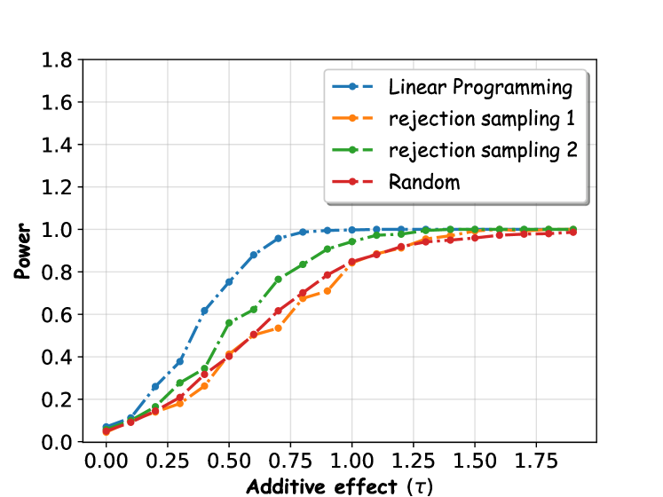
(a) $m=3$

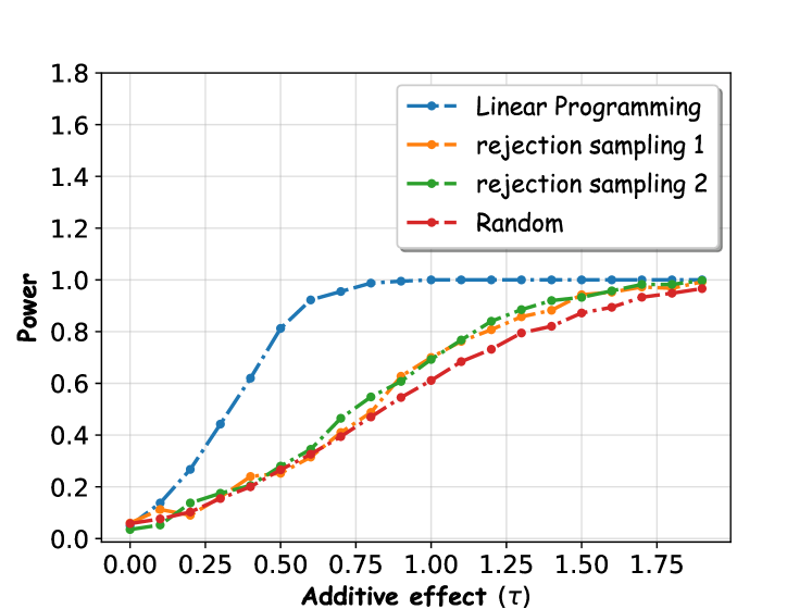
(b) $m=4$

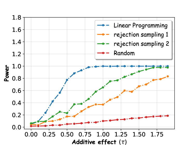
(c) $m=5$

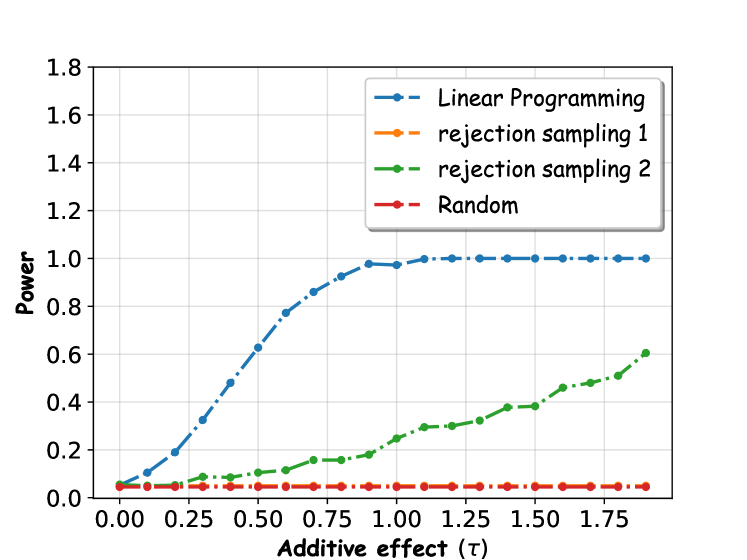
(d) $m=6$

Figure 2: Power against additive effect for different group sizes

In all simulations, we use the randomization procedure described in Definition 2, but we vary the choice of the initial $C_{0}$ — different choices lead to different designs. We compare the optimal initialization strategy of Section 5 with three alternative initialization strategies to assign $C$:

1. Rejection sampling 1: The best initialization in $M=10$ random permutations of the initial $C_{0}$

2. Rejection sampling 2: The best initialization in $M=1000$ random permutations of the initial $C_{0}$

3. Random initialization: A random permutation of the initial $C_{0}$

More details on the simulation setup can be found in the Supplementary Material. The results of our simulations are plotted in Figure 2.

In our simulation, optimal design using linear programming leads to more powerful tests than the other initializations for all additive effects and group sizes we considered. The benefits of our linear programming strategy grow starker as the size of the groups increases; indeed, for $m=6$, our optimal design leads to tests that have a power of $1$ against the alternative $\tau=1$, while the best alternative initialization strategy leads to tests of power less than $0.3$. This is because as group size increases, the number of possible exposures increases significantly and it is much more difficult for brute force algorithm with a fixed number of iterations to find a near-optimal solution.

Appendix A Proof of the main results

A.1 Elements of group theory

Throughout this section, recall that $C=(C_{1},\ldots,C_{N})\in\mathbb{C}$, where $C_{i}=(L_{i},W_{i})$ is the pair of group assignment and additional intervention assignment.

Definition 3 (Group action on a set).

Consider a permutation group $\Pi$ and a finite set of $N$-vector pairs, $\mathbb{C}$. A group action of $\Pi$ on $\mathbb{C}$ is a mapping $\phi:\Pi\times\mathbb{C}\to\mathbb{C}$ (usually we write $\pi\cdot C$ instead of $\phi(\pi,C)$) satisfying the following:

1. for all $C\in\mathbb{C}$, $e\cdot C=C$ where $e$ is the identity element of $\Pi$;

2. for all $\pi,\pi^{\prime}\in\Pi$, and all $C\in\mathbb{C}$, $\pi^{\prime}\cdot(\pi\cdot C)=(\pi^{\prime}\pi)\cdot C$

It can be checked that for $\pi\in S$ and $C=(C_{1},\ldots,C_{N})\in\mathbb{C}$, the mapping $\pi\cdot C=(C_{\pi^{-1}(i)})_{i=1}^{N}=(L_{\pi^{-1}(i)},W_{\pi^{-1}(i)})_{i=1}^{N}$ is a group action.

Definition 4 (Orbits and stabilizers).

Let $\Pi$ be a permutation group and $\mathbb{C}$ a finite set of $N$-vectors. If $C\in\mathbb{C}$, the orbit of $C$ under $\Pi$ is defined as

$$\Pi\cdot C\equiv\{\pi\cdot C:\pi\in\Pi\},$$

and the stabilizer of $C$ in $\Pi$ is defined as

$$\Pi_{C}\equiv\{\pi\in\Pi:\pi\cdot C=C\}.$$

Recall the definition of a transitive group action in the main text.

Definition 5 (Transitivity).

A subgroup $\Pi\subset S$ of the symmetric group $S$ acts transitively on $\mathbb{C}$ if $\mathbb{C}=\Pi\cdot C$ for any $C\in\mathbb{C}$.

We will now state a version of the Orbit-Stabilizer Theorem that will is specific to our setup.

Theorem 4 (Orbit-Stabilizer).

Let $\Pi$ be a permutation group acting transitively on a finite set of $N$-vectors $\mathbb{C}$.

1. For all $C,C^{\prime}\in\mathbb{C}$, $|\Pi_{C}|=|\Pi_{C^{\prime}}|=D$ a constant. In words, it means that all stabilizers have the same size.

2. We already know that for all $C\in\mathbb{C}$, $\Pi\cdot C=\mathbb{C}$. We also have:

   $$|\Pi\cdot C|=\frac{|\Pi|}{|\Pi_{C}|}=\frac{|\Pi|}{D}.$$

A.2 Proof of Theorem 1

Theorem 1. If $\textup{pr}(C)$ is generated from the randomization procedure in Definition 2, then the induced distribution of exposure $\textup{pr}(H)$ is $SCRD(\mathbf{n}_{A})$.

The proof for Theorem 1 can be split into two parts. The first part is about showing equivariance of exposure mapping under permutation of latent assignments, and the second part is about establishing symmetry property.

Lemma 1.

Let $\Pi$ be a subgroup of $S_{A}$, the stabilizer of the attribute vector $A$ in $S$. For $C\in\mathbb{C}\subset\{1,\ldots,K\}^{N}\times\mathcal{W}^{N}$, define $h^{*}(C)=h(W,Z(L))$, where $h_{i}(W,Z(L))=\{W_{i}\}\cup\{(A_{j},W_{j}),j\in Z_{i}\}\}$ is the exposure mapping of unit $i$ and domain $\mathbb{H}=\{h^{*}(C):C\in\mathbb{C}\}$. Then we have that $h^{*}:\mathbb{C}\to\mathbb{H}$ is equivariant with respect to $\Pi$.

Proof.

We will show that $h^{*}(\pi\cdot C)=\pi\cdot h^{*}(C)$ for all $C\in\mathbb{C}$ and all $\pi\in\Pi$.

Consider a fixed $C\in\mathbb{C}$ and $\pi\in\Pi$. By definition, we have

$$[h^{*}(C)]_{i}=\{W_{i}\}\cup\{(A_{j},W_{j}):j\neq i,L_{j}=L_{i}\}.$$

Then we have for all $i\in\mathbb{I}$,

$$[h^{*}(\pi\cdot C)]_{i} =\{[\pi\cdot W]_{i}\}\cup\{([\pi\cdot A]_{j},[\pi\cdot W]_{j}):j\neq i,[\pi\cdot L]_{j}=[\pi\cdot L]_{i}\}$$

$$=\{W_{\pi^{-1}(i)}\}\cup\{(A_{\pi^{-1}(j)},W_{\pi^{-1}(j)}):j\neq i,L_{\pi^{-1}(j)}=L_{\pi^{-1}(i)}\}$$

$$=\{W_{\pi^{-1}(i)}\}\cup\{(A_{j},W_{\pi^{-1}(j)}):j\neq i,L_{\pi^{-1}(j)}=L_{\pi^{-1}(i)}\}$$

$$=\{W_{\pi^{-1}(i)}\}\cup\{(A_{\pi(\pi^{-1}(j))},W_{\pi^{-1}(j)}):\pi(\pi^{-1}(j))\neq i,L_{\pi^{-1}(j)}=L_{\pi^{-1}(i)}\}$$

$$=\{W_{\pi^{-1}(i)}\}\cup\{(A_{\pi(j^{\prime})},W_{j^{\prime}}):j^{\prime}\neq\pi^{-1}(i),L_{j^{\prime}}=L_{\pi^{-1}(i)}\}$$

$$=\{W_{\pi^{-1}(i)}\}\cup\{(A_{j^{\prime}},W_{j^{\prime}}):j^{\prime}\neq\pi^{-1}(i),L_{j^{\prime}}=L_{\pi^{-1}(i)}\}$$

$$=[h^{*}(C)]_{\pi^{-1}(i)}$$

$$=[\pi\cdot h^{*}(C)]_{i}$$

∎

Lemma 1 shows that exposure mapping is equivariant with respect to simultaneous permutation of the group and external intervention treatment assignments. In other words, permuting the latent assignment vector $C$ is equivalent to permuting the exposure mappings. This allows symmetry properties to propagate from latent assignments to the induced exposure distribution. Specifically, we focus on designs for which the exposure has a Stratified Completely Randomized Design. Recall the notion of $\operatorname{SCRD}(\mathbf{n}_{A})$ in Definition 1.

Definition 1. Without loss of generality, denote by $\mathcal{H}$ the set of possible exposures and $A$ an N-vector. Let $\mathbf{n}_{A}=(n_{a,h})_{a\in\mathcal{A},h\in\mathcal{H}}$, such that $\sum_{h\in\mathcal{H}}n_{a,h}=N_{[a]}$, denote a vector of non-negative integers corresponding to number of units with each possible attribute and exposure combination. We say that a distribution of exposures $\textup{pr}(H)$ is a stratified completely randomized design denoted by $\operatorname{SCRD}(\mathbf{n}_{A})$ if the following two conditions are satisfied.

1. After stratifying based on $A$, the exposure $H=(H_{1},\ldots,H_{N})$ is completely randomized. That is, (1) $\mathbb{P}(H_{i}=h)=\mathbb{P}(H_{j}=h)$ for all $h\in\mathcal{H}$ and $i,j\in\mathbb{I}$ such that $A_{i}=A_{j}$; (2) the number of units with exposure $h\in\mathcal{H}$ and stratum $a\in\mathcal{A}$ is $n_{a,h}$.

2. The exposure assignments across strata are independent. That is $\mathbb{P}(H_{i}=h_{i}|H_{j}=h_{j})=\mathbb{P}(H_{i}=h_{i})$ for all $h_{i},h_{j}\in\mathcal{H}$ and $i,j\in\mathbb{I}$ such that $A_{i}\neq A_{j}$.

Lemma 2.

Fix any $H_{0}\in\mathbb{H}=\{h^{*}(C):C\in\mathbb{C}\}$ and generate $H=\pi\cdot H_{0}$ where $\pi\sim\operatorname{Unif}(S_{A})$. Then the distribution of exposures $\textup{pr}(H)$ is $\operatorname{SCRD}(\mathbf{n}_{A})$.

Proof.

We first note that if we permute $H$ by $\pi\in\operatorname{Unif}(S)$, then $\textup{pr}(H)$ is completely randomized (CRD). This is because with a random permutation, $\mathbb{P}(H_{i}=h)=\mathbb{P}(H_{j}=h)$ for all $h\in\mathcal{H}$. We then proceed by proving the two conditions in the definition for $\operatorname{SCRD}(\mathbf{n}_{A})$ separately.

1. We will show that $\textup{pr}(H)$ satisfies completely randomized design (CRD) within each stratum defined by attribute vector $A$, i.e. $\mathbb{P}(H_{i}=h)=\mathbb{P}(H_{j}=h)$ for all $h\in\mathcal{H}$ and $i,j\in\mathbb{I}$ such that $A_{i}=A_{j}$.

   For each stratum $k$ as defined from $A$, let

   $$I_{k}\equiv\{i\in\mathbb{I}:A_{i}=k\}.$$

   For $\pi\in S_{A}$, let $\tilde{\pi}^{(k)}:I_{k}\mapsto\mathbb{I}$ be the restriction of $\pi$ to $I_{k}$ such that $\tilde{\pi}^{(k)}(i)=\pi(i)$. Since $\pi\in S_{A}$, $\pi(i)\in I_{k}$, $\forall i\in I_{k}$. Therefore $\operatorname{Img}(\tilde{\pi}^{(k)})\subset I_{k}$. But since $\pi$ is a permutation, $\tilde{\pi}^{(k)}$ is a bijection. Therefore $\operatorname{Img}(\tilde{\pi}^{(k)})=I_{k}$. This shows that $\tilde{\pi}^{(k)}\in S^{k}$ where $S^{k}$ is the symmetric group on $I_{k}$.

   We then characterize the induced distribution of $\tilde{\pi}^{(k)}$ on $S^{k}$, where we sample $\pi\sim\operatorname{Unif}(S_{A})$. Define the following $N$-vector $L^{k}=(L_{1}^{k},\ldots,L_{N}^{k})$ where

   $$L_{i}^{k}=\begin{cases}0,&\text{ if }i\notin I_{k}\\ i,&\text{ if }i\in I_{k}.\end{cases}$$

   For any $\pi^{*}\in S^{k}$, we have

   $$\textup{pr}(\pi^{*}) =\sum_{\pi\in S_{A}}1\{\tilde{\pi}^{(k)}=\pi^{*}\}\frac{1}{|S_{A}|}$$

   $$=\frac{|S_{AL^{k}}|}{|S_{A}|}$$

   $$=\frac{1}{|S_{A}\cdot L^{k}|},$$

   where the last line is due to the Orbit-Stabilizer Theorem. We will further show that $|S_{A}\cdot L^{k}|=|S^{k}|$.

   For any $\pi\in S_{A}$, $(\pi\cdot L^{k})_{i}\notin I_{k}$, $\forall i\notin I_{k}$. By the definition of $L^{k}$, we know that $(\pi\cdot L^{k})_{i}=L_{i}^{k}=0$, $\forall i\notin I_{k}$. Therefore

   $$|S_{A}\cdot L^{k}|\leq|I_{k}|!=|S^{k}|.$$

   For the opposite inequality, consider any permutations $\pi\in S_{k}$ acting on $L^{k}$ restricted to $I_{k}$. Define the extended permutation $\tilde{\pi}$ on $\mathbb{I}$ by

   $$\tilde{\pi}(i)=\begin{cases}i,&i\notin I_{k}\\ \pi(i)&i\in I_{k},\end{cases}$$

   and denote the set of all such $\tilde{\pi}$ as $\tilde{S}^{k}$. Since $L_{i}^{k}\neq L_{j}^{k}$, $\forall i\neq j$ and $i,j\in I_{k}$, $|\tilde{S}^{k}\cdot L^{k}|=|S^{k}|$. Since by construction, $\tilde{S}^{k}\subset S_{A}$, we have that

   $$|S_{A}\cdot L^{k}|\geq|\tilde{S}^{k}\cdot L^{k}|=|S^{k}|.$$

   Combining the two inequalities together, we have

   $$\textup{pr}(\pi^{*})=\frac{1}{|S_{A}\cdot L^{k}|}=\frac{1}{|S^{k}|}.$$

   This implies that the induced restricted permutations $\tilde{\pi}^{(k)}\sim\operatorname{Unif}(S^{k})$ for all $k$. In other words, $\textup{pr}(H)$ satisfies CRD within each stratum $k$, and hence $\mathbb{P}(H_{i}=h)=\mathbb{P}(H_{j}=h)$ for all $h\in\mathcal{H}$ and $i,j\in\mathbb{I}$ such that $A_{i}=A_{j}$.

2. We will show that exposure assignments are independent across strata. First notice that for all $h_{i},h_{j}\in\mathcal{H}$ and $i,j\in\mathbb{I}$ such that $A_{i}\neq A_{j}$,

   $$\mathbb{P}(H_{i}=h_{i}|H_{j}=h_{j}) =\mathbb{P}((\pi\cdot H_{0})_{i}=h_{i}|(\pi\cdot H_{0})_{j}=h_{j})$$

   $$=\mathbb{P}(\pi(i)\in D|\pi(j)\in E),$$

   for some disjoint sets $D,E\subset\mathbb{I}$ such that $D\subset I_{A_{i}}$ and $E\subset I_{A_{j}}$. By Baye’s rule we have,

   $$\mathbb{P}(\pi(i)\in D|\pi(j)\in E) =\frac{\mathbb{P}(\pi(i)\in D,\pi(j)\in E)}{\mathbb{P}(\pi(j)\in E)}$$

   $$=\frac{\mathbb{P}(\pi(i)\in D,\pi(j)\in E)}{\sum_{i^{*}\in I_{A_{i}}}\mathbb{P}(\pi(i)=i^{*},\pi(j)\in E)}$$

   $$=\frac{|D|}{|I_{A_{i}}|},$$

   where last equality is because $\mathbb{P}(\pi(i)=i^{*},\pi(j)\in E)$ is the same for all $i^{*}\in I_{A_{i}}$. Finally we have

   $$\mathbb{P}(H_{i}=h_{i}|H_{j}=h_{j})=\frac{|D|}{|I_{A_{i}}|}=\mathbb{P}(\pi(i)\in D)=\mathbb{P}(H_{i}=h_{i}),$$

   where the second equality is due to CRD within $I_{A_{i}}$ in part $(1)$.

∎

Combining the above two Lemmas together proves Theorem 1 that $\textup{pr}(H)$ is $\operatorname{SCRD}(\textbf{n}_{A})$.

A.3 Proof of Proposition 1

Proposition 1. Consider observed $N-$vectors of exposure $H^{obs}\sim\textup{pr}(H)$ and outcome $Y^{obs}=Y(H^{obs})$, resulting in focal set $\mathcal{U}^{obs}$ and test statistic $T^{obs}=T(H^{obs},Y^{obs},\mathcal{U}^{obs})$. If $H^{\prime}\sim\textup{pr}(H|\mathcal{U}^{obs})$ and $T^{\prime}=T(H^{\prime},Y^{obs},\mathcal{U}^{obs})$, then the following quantity,

$$\operatorname{pval}(H^{obs})=\textup{pr}(T^{\prime}\geq T^{obs}|\mathcal{U}^{obs})$$

is a valid p-value conditionally and marginally for $H_{0}^{(\gamma_{1},w_{1}),(\gamma_{2},w_{2})}$. That is, if $H_{0}^{(\gamma_{1},w_{1}),(\gamma_{2},w_{2})}$ is true, then for any $\mathcal{U}^{obs}$ and $\alpha\in[0,1]$, we have $\textup{pr}\{\operatorname{pval}(H^{obs})\leq\alpha|\mathcal{U}^{obs}\}\leq\alpha$.

Proof.

Recall that $u(Z(L),W)=\{i\in\mathbb{I}:(h_{i}(Z(L),W),W_{i})\in\{(\gamma_{1},w_{1}),(\gamma_{2},w_{2})\}\}$. Define $m(\mathcal{U}|C)=\mathds{1}\{u(Z(L),W)=\mathcal{U}\}$. Then,

$$m(\mathcal{U}|C)>0\Rightarrow u(Z(L),W)=\mathcal{U}\Rightarrow h_{i}(Z(L),W)\in\{(\gamma_{1},w_{1}),(\gamma_{2},w_{2})\},\forall i\in\mathcal{U}.$$

Therefore $\textup{pr}(C|\mathcal{U})>0$ implies that $\textup{pr}(\mathcal{U}|C)>0$, and hence
$h_{i}(Z(L),W)\in\{(\gamma_{1},w_{1}),(\gamma_{2},w_{2})\},\forall i\in\mathcal{U}$. For all $C,C^{\prime}$ such that $\textup{pr}(C|\mathcal{U})>0$ and $\textup{pr}(C^{\prime}|\mathcal{U})>0$, we must have $h_{i}(Z(L),W),h_{i}(Z(L^{\prime}),W^{\prime})\in\{(\gamma_{1},w_{1}),(\gamma_{2},w_{2})\},\forall i\in\mathcal{U}$. Therefore under the null hypothesis $H_{0}^{(\gamma_{1},w_{1}),(\gamma_{2},w_{2})}$, $Y_{i}(Z(L),W)=Y_{i}(Z(L^{\prime}),W^{\prime})=Y_{i}(\gamma_{1},w_{1})=Y_{i}(\gamma_{2},w_{2})$. This means that under $H_{0}^{(\gamma_{1},w_{1}),(\gamma_{2},w_{2})}$, the test statistic $T$ is imputable. The result then follows from Theorem 2.1 of Basse et al. (2019). ∎

A.4 Proof of Theorem 3

Theorem 3. Let $\textup{pr}(C)$ be generated from randomization procedure described in Definition 2 and $\textup{pr}(H)$ the induced exposure distribution. Define a focal set $\mathcal{U}=u(Z,W)=\{i\in\mathbb{I}:h_{i}(Z,W)\in\mathcal{H}_{u}\}$ for some $pr(W,Z)>0$ and set of exposures $\mathcal{H}_{u}\subset\mathcal{H}$. Let $U=(U_{1},\ldots,U_{N})$, where $U_{i}=\mathds{1}(i\in\mathcal{U})$. Then the conditional distribution of exposure, $pr(H|\mathcal{U})$, is $SCRD(\mathbf{n}_{A\mathcal{U}})$.

In order to prove Theorem 3, we need to introduce concepts of group symmetry and then establish the connection between group symmetry and $SCRD(\mathbf{n}_{A\mathcal{U}})$.

Definition 6 ($\Pi$-symmetry).

Let $\Pi\subset S$ be a subgroup of the symmetric group $S$. A distribution, $\textup{pr}(H)$ with domain $\mathbb{H}$ is called $\Pi$-symmetric if $\textup{pr}(H)=\operatorname{Unif}(\mathbb{H})$ and $\Pi$ acts transitively on $\mathbb{H}$.

The following Proposition establishes connections between $\Pi$-symmetry and sampling procedure.

Proposition 2.

Let $\Pi\subset S$ be a subgroup of the symmetric group $S$ and $\mathbb{H}=\{h^{*}(C):C\in\mathbb{C}\}$. Take any $H_{0}\in\mathbb{H}$ and define $\mathbb{H}_{0}=\Pi\cdot H_{0}$.

1. If we sample $H=\pi\cdot H_{0}$, where $\pi\sim\operatorname{Unif}(\Pi)$, then the distribution of $H$ is $\Pi$-symmetric on $\mathbb{H}_{0}$.

2. If a distribution of $H$ is $\Pi$-symmetric on its domain $\mathbb{H}_{0}$, then it can be generated by sampling $H=\pi\cdot H_{0}$, where $\pi\sim\operatorname{Unif}(\Pi)$.

Proof.

The proof for part (1) and part (2) are identical. The definition of $\Pi$-symmetry involves two parts, namely transitivity and uniform distribution on the support. We first show that $\Pi$ acts transitively on the set $\mathbb{H}_{0}$, that is for all $H\in\mathbb{H}_{0}$, $\Pi\cdot H=\mathbb{H}_{0}$.

By construction, for all $H\in\mathbb{H}_{0}$, there exists $\pi_{0}\in\Pi$ such that $H=\pi_{0}\cdot H_{0}$. Therefore transitivity condition of $\Pi\cdot H=\mathbb{H}_{0}$ can also be written as

$$(\Pi\pi_{0})\cdot H_{0}=\Pi\cdot H_{0}.$$

To prove transitivity, it then suffices to show that $\Pi\pi_{0}=\Pi$.

Since for all $\pi\in\Pi\pi_{0}$, there exists $\pi^{\prime}\in\Pi$ such that $\pi=\pi^{\prime}\pi_{0}\in\Pi$, we have $\Pi\pi_{0}\subset\Pi$. For the reverse direction, consider $\pi\in\Pi$, we can expand $\pi=\pi\pi_{0}^{-1}\pi_{0}\in\Pi\pi_{0}$ since $\pi\pi_{0}^{-1}\in\Pi$. Therefore $\Pi\pi_{0}=\Pi$ and hence transitivity holds.

Before moving on to the second part, we first clarify some notations. Define $\textup{pr}_{\Pi}(\pi)=\operatorname{Unif}(\Pi)$ and $\textup{pr}_{\Pi,H_{0}}(H)$ the distribution of $H$ generated by the sampling procedure: that is, the distribution of $H$ obtained by first sampling $\pi$ from $\textup{pr}_{\Pi}(\pi)$ and then applying $\pi\cdot H_{0}$. It remains to prove that $\textup{pr}_{\Pi,H_{0}}(H)=\operatorname{Unif}(\mathbb{H}_{0})$.

Again we have for any $H\in\mathbb{H}_{0}$, there exists $\pi_{0}\in\Pi$ such that $H=\pi_{0}\cdot H_{0}$. This means that $H_{0}=\pi_{0}^{-1}\cdot H$ for some $\pi_{0}^{-1}\in\Pi$. Therefore

$$\textup{pr}_{\Pi,H_{0}}(H) =\sum_{\pi\in\Pi}\mathds{1}(\pi\cdot H_{0}=H)\textup{pr}_{\Pi}(\pi)$$

$$=\sum_{\pi\in\Pi}\mathds{1}(\pi\cdot(\pi_{0}^{-1}\cdot H)=H)\textup{pr}_{\Pi}(\pi)$$

$$=\sum_{\pi\in\Pi}\mathds{1}((\pi\pi_{0}^{-1})\cdot H=H)\textup{pr}_{\Pi}(\pi)$$

$$=\sum_{\pi\in\Pi}\mathds{1}(\pi\pi_{0}^{-1}\in\Pi_{H})\textup{pr}_{\Pi}(\pi)$$

$$=\sum_{\pi\in\Pi}\mathds{1}(\pi\in\Pi_{H}\pi_{0})\textup{pr}_{\Pi}(\pi)$$

$$=\textup{pr}_{\Pi}(\Pi_{H}\pi_{0}),$$

where $\Pi_{H}$ is the stabilizer of $H$ in $\Pi$. Since $\textup{pr}_{\Pi}(\pi)=\operatorname{Unif}(\Pi)$ and $\Pi_{H}\pi_{0}\subset\Pi$, we have

$$\textup{pr}_{\Pi,H_{0}}(H)=\textup{pr}_{\Pi}(\Pi_{H}\pi_{0})=\frac{|\Pi_{H}\pi_{0}|}{|\Pi|}.$$ (3)

We quickly verify that $|\Pi_{H}\pi_{0}|=|\Pi_{H}|$. Clearly, $|\Pi_{H}\pi_{0}|\leq|\Pi_{H}|$ and we only need to verify the other direction. Suppose that there exist $\pi_{1},\pi_{2}\in\Pi_{H}$ such that $\pi_{1}\neq\pi_{2}$ but $\pi_{1}\pi_{0}=\pi_{2}\pi_{0}$. Then this would imply

$$\pi_{1}\pi_{0}\pi_{0}^{-1}=\pi_{2}\Longrightarrow\pi_{1}=\pi_{2},$$

which is a contradiction. Since $\pi_{1}\neq\pi_{2}$ implies $\pi_{1}\pi_{0}\neq\pi_{2}\pi_{0}$, we know that $|\Pi_{H}\pi_{0}|\geq|\Pi_{H}|$. Therefore $|\Pi_{H}\pi_{0}|=|\Pi_{H}|$. Applying this to Equation (3), we have

$$\textup{pr}_{\Pi,H_{0}}(H)=\frac{|\Pi_{H}|}{|\Pi|}.$$

By the Orbit-Stabilizer Theorem, $|\Pi\cdot H|=|\Pi|/|\Pi_{H}|$. Therefore

$$\textup{pr}_{\Pi,H_{0}}(H)=|\Pi\cdot H|^{-1}=|\mathbb{H}_{0}|^{-1}=\operatorname{Unif}(\mathbb{H}_{0}),$$

where the second equality is due to transitivity that we proved earlier. Therefore $\textup{pr}_{\Pi,H_{0}}(H)$ is $\Pi$-symmetric on $\mathbb{H}_{0}$. ∎

We now proceed to prove Theorem 3 in two steps. The first step tries to characterize symmetry property of $\textup{pr}(H|\mathcal{U})$ and the second step relates symmetry property to $SCRD(\mathbf{n}_{A\mathcal{U}})$.

Proposition 3.

Let $\textup{pr}(C)$ be generated from randomization procedure in Definition 2 and $\textup{pr}(H)$ the induced exposure distribution. Define a focal set $\mathcal{U}=u(Z,W)=\{i\in\mathbb{I}:h_{i}(Z,W)\in\mathcal{H}_{u}\}$ for some $pr(W,Z)>0$ and set of exposures $\mathcal{H}_{u}\subset\mathcal{H}$. Let $U=(U_{1},\ldots,U_{N})$, where $U_{i}=\mathds{1}(i\in\mathcal{U})$. Then the conditional distribution of exposure, $pr(H|\mathcal{U})$, is $S_{AU}-$symmetric, where $S_{AU}$ is the stabilizer of both $A$ and $U$ in $S$.

Proof.

First recall that due to equivariance in Lemma 1, the induced $\textup{pr}(H)$ is generated by sampling $H=\pi\cdot H_{0}$, where $\pi\in S_{A}$. By first part of Proposition 2, we know that the distribution of exposures $\textup{pr}(H)$ is $S_{A}$-symmetric on its domain $\mathbb{H}$. In particular, it has a uniform distribution on $\mathbb{H}$.

Notice that the function $u(\cdot)$ depends on $(W,Z)$ only through $H=h(W,Z)$. This makes it possible to define another function $m(\cdot)$ such that $\mathcal{U}=m(H)=m(h(W,Z))=u(W,Z)$. Since there is a one-to-one mapping between $\mathcal{U}$ and $U$, we can use the two notations interchangeably. The reason that $U$ is a useful representation is that it is an $N-$vector, allowing previous notations of permutation to work out. Here we can write $U=m(H)$.

We have

$$pr(H|\mathcal{U}) \propto pr(\mathcal{U}|H)pr(H)$$

$$\propto pr(\mathcal{U}|H)\text{ since $pr(H)=\operatorname{Unif}(\mathbb{H})\propto 1$}$$

$$\propto\mathds{1}\{m(H)=U\},$$

which implies that $pr(H|\mathcal{U})=\operatorname{Unif}\{\mathbb{H}(U)\}$ on the support

$$\mathbb{H}(U)=\{H\in\mathbb{H}:m(H)=U\}.$$

Now notice that for all $\pi\in S_{A}$ and any exposure set of interest $h_{1}$, $h_{2}$, we have

$$[m(\pi\cdot H)]_{i} =\mathds{1}\left([\pi\cdot H]_{i}\in\mathcal{H}_{u}\right)$$

$$=\mathds{1}\left(H_{\pi^{-1}(i)}\in\mathcal{H}_{u}\right)$$

$$=[m(H)]_{\pi^{-1}(i)}$$

$$=[\pi\cdot m(H)]_{i},$$

that is, $m$ is equivariant, $m(\pi\cdot H)=\pi\cdot m(H)$. Let $H_{0}\in\mathbb{H}(U)$ such that $m(H_{0})=U$. We have,

$$\mathbb{H}(U) =\{H\in\mathbb{H}:m(H)=U\}$$

$$=\{\pi\cdot H_{0}:\pi\in S_{A},m(\pi\cdot H_{0})=U\},\text{ since $S_{A}$ is transitive on $\mathbb{H}$}$$

$$=\{\pi\cdot H_{0}:\pi\in S_{A},\pi\cdot m(H_{0})=U\},\text{ due to equivariance}$$

$$=\{\pi\cdot H_{0}:\pi\in S_{A},\pi\cdot U=U\}$$

$$=S_{AU}\cdot H_{0}.$$

This shows that $S_{AU}$ is transitive on $\mathbb{H}(U)$, the support of $\textup{pr}(H|\mathcal{U})$. Having shown earlier that $\textup{pr}(W|\mathcal{U})=\operatorname{Unif}\{\mathbb{H}(U)\}$, we therefore conclude that $\textup{pr}(H|\mathcal{U})$ is $S_{AU}$-symmetric on its support. ∎

Since $\textup{pr}(H|\mathcal{U})$ is $S_{AU}$-symmetric on its support $\mathbb{H}(U)$, we know by part (2) of Proposition 2, $\textup{pr}(H|\mathcal{U})$ can be generated by sampling $H=\pi\cdot H_{0}$, where $\pi\sim\operatorname{Unif}(S_{AU})$. Then the second step is to invoke Lemma 2 in proof of Theorem 1 except that we replace the $N$-vector $A$ with $AU$ where $(AU)_{i}=(A_{i},U_{i})$. This completes the proof that $\textup{pr}(H|\mathcal{U})$ is $SCRD(\mathbf{n}_{A\mathcal{U}})$.

Appendix B Testing for sharp null hypothesis

Consider testing the global null hypothesis

$$H_{0}:Y_{i}(\gamma_{1},w_{1})=Y_{i}(\gamma_{2},w_{2}),\forall(\gamma_{1},w_{1}),(\gamma_{2},w_{2})\in\mathcal{H},\forall i\in\mathbb{I},$$

which asserts that the combined intervention has no effect whatsoever on any unit. We illustrate here how the classical Fisher Randomization Test can be applied to test this sharp null hypothesis.

Proposition 4.

Consider observed assignment $C^{obs}\sim\textup{pr}(C)$.

1. Observe outcomes, $Y^{obs}=Y(C^{obs})=Y(Z(L^{obs}),W^{obs})$, where $C^{obs}_{i}=(L^{obs}_{i},W^{obs}_{i})$ for all $i\in\mathbb{I}$.

2. Compute $T^{obs}=T(C^{obs},Y^{obs})$.

3. For $C^{\prime}\sim\textup{pr}(C)$, let $T^{\prime}=T(C^{\prime},Y^{obs})$ and define:

   $$\operatorname{pval}(C^{obs})=\textup{pr}(T^{\prime}\geq T^{obs}),$$

   where $T^{obs}$ is fixed and the randomization distribution is with respect to $\textup{pr}(Z^{\prime})$.

Then the p-value of $\operatorname{pval}(C^{obs})$ is valid. That is, if $H_{0}$ is true, then $\textup{pr}\{\operatorname{pval}(C^{obs})\leq\alpha\}\leq\alpha$.

Appendix C Balance in optimal design heuristics

The naive approach in section 5 only considers the objective of maximizing the total number of units with both target exposures, without requiring balance between the two exposures. We will show how to reformulate the optimization to incorporate balance by adding various constraints. But before that, we want to point out the subtleties in incorporating balance as well as the caveats in incorporating balance in the wrong way or simply ignoring it.

Recall that the randomizations in Definition 2 are permutations that are in the stabilizer of attribute $A$. This suggests that balance between the two target exposures should be taken into consideration within each category of attribute instead of on the global level across all attribute values. In fact, considering balance between the two target exposures without taking into account of diversity within each attribute class could result in greedy choice that leads to zero power. For example, if all units with the first target exposure are of attribute $a_{1}\in\mathcal{A}$ while all units with the second target exposure are of attribute $a_{2}\in\mathcal{A}$ for $a_{1}\neq a_{2}$, then permutations in the stabilizer of $A$ do not change the test statistics at all. In this worst case, we will have zero power. Similarly, in the naive approach that neglects the balance between the two target exposures, the same worst case scenarios may happen resulting in zero power.

It is worth noting that the correct way to incorporate balance and the heuristics for maximizing power of randomization tests also coincide with the goal of minimizing variance in estimations. From standard theory about estimation of variance, it can be seen that variance estimator is small if the denominators $n_{[a]\gamma,w}$ and $n_{[a]\gamma^{\prime},w^{\prime}}$ are large for both target exposures $(\gamma,w)$ and $(\gamma^{\prime},w^{\prime})$ within attribute class $a\in\mathcal{A}$. This suggests that an optimal design desires large values of both $n_{[a]\gamma,w}$ and $n_{[a]\gamma^{\prime},w^{\prime}}$, which can be implemented by maximizing the sum of units with both target exposures, subject to the within-attribute balance constraints. We will now formally state the reformulation of the integer linear programming problem.

Given target exposures $(\gamma_{1},w_{1})$ and $(\gamma_{2},w_{2})$, we know the exact composition of attribute-intervention pair of the neighbors of all units with target treatments. This allows us to enumerate all elements in $\mathcal{G^{*}}$ and hence pre-compute the constants $m_{1}(G_{i})$, $m_{2}(G_{i})$, and $c_{j}(G_{i})$ for all $G_{i}\in\mathcal{G^{*}}$ and $j\in\mathcal{A}$.

Assume without loss of generality that $\mathcal{A}=\{0,1\}$. Define the following additional constants

$$A_{1}(G_{i})=\begin{cases}1,&\text{if the units with exposure $1$ in group design $G_{i}$}\\ &\text{has attribute $1$ and }n_{1}(G_{i})>0\\ 0,&\text{if the units with exposure $1$ in group design $G_{i}$}\\ &\text{has attribute $0$ and }n_{1}(G_{i})>0\\ \text{anything}&\text{otherwise}.\end{cases}$$

And similarly,

$$A_{2}(G_{i})=\begin{cases}1,&\text{if the units with exposure $2$ in group design $G_{i}$}\\ &\text{has attribute $1$ and }n_{2}(G_{i})>0\\ 0,&\text{if the units with exposure $2$ in group design $G_{i}$}\\ &\text{has attribute $0$ and }n_{2}(G_{i})>0\\ \text{anything}&\text{otherwise}.\end{cases}$$

Therefore the heuristic for maximizing power of the Fisherian inference can be translated as the following optimization problem.

$$\operatorname{argmax}_{\{n_{i}\}} \sum_{G_{i}\in\mathcal{G^{*}}}n_{i}(m_{1}(G_{i})+m_{2}(G_{i}))$$

$$\operatorname{s.t.} \sum_{G_{i}\in\mathcal{G^{*}}}n_{i}c_{1}(G_{i})\leq n_{[1]}$$

$$\sum_{G_{i}\in\mathcal{G^{*}}}n_{i}c_{0}(G_{i})\leq N-n_{[1]}$$

$$\sum_{G_{i}\in\mathcal{G^{*}}}n_{i}m_{1}(G_{i})A_{1}(G_{i})\leq\eta\cdot\sum_{G_{i}\in\mathcal{G^{*}}}n_{i}m_{2}(G_{i})A_{2}(G_{i})$$

$$\sum_{G_{i}\in\mathcal{G^{*}}}n_{i}m_{2}(G_{i})A_{1}(G_{i})\leq\eta\cdot\sum_{G_{i}\in\mathcal{G^{*}}}n_{i}m_{1}(G_{i})A_{2}(G_{i})$$

$$\sum_{G_{i}\in\mathcal{G^{*}}}n_{i}m_{1}(G_{i})(1-A_{1}(G_{i}))\leq\eta\cdot\sum_{G_{i}\in\mathcal{G^{*}}}n_{i}m_{2}(G_{i})(1-A_{2}(G_{i}))$$

$$\sum_{G_{i}\in\mathcal{G^{*}}}n_{i}m_{2}(G_{i})(1-A_{1}(G_{i}))\leq\eta\cdot\sum_{G_{i}\in\mathcal{G^{*}}}n_{i}m_{1}(G_{i})(1-A_{2}(G_{i}))$$

$$n_{i}\geq 0,n_{i}\in\mathbb{Z},\forall n_{i},$$

where $\eta=1+\epsilon$ for some $\epsilon>0$ that can be chosen to achieve a satisfiable trade-off between the two objectives of maximizing total number and balancing. This is in the standard form of an integer linear programming problem or a knapsack problem in particular. The general case for attribute value set $|\mathcal{A}|>2$ can be extended directly from this binary attribute case.

Remark 1.

The heuristics for maximizing power is qualitative and hence the above optimization problem is just one of many ways to realize the heuristic. For example, the tuning parameter $\eta$ can be adjusted by the practitioner to achieve different tradeoffs for maximizing number of units with target treatment and balancing between the two treatments. Different values of $\eta$ can also be used for different balancing constraints as well.

Remark 2.

Integer linear programing problems are NP-hard and there are established iterative solvers that yield good approximations of the true optimizer. However, in this case, we can get fairly good approximation of the optimal assignment by simply taking one step of linear programming relaxation and rounding downwards. That is, we drop the constraint that $n_{i}\in\mathbb{Z}$ and solve the simple linear programing problem. Since we are rounding downwards and all coefficients are non-negative, the round-off integer solution is still feasible. This one-step linear relaxation has the advantage that it gives a fast initialization yielding near optimal power among all possible initializations. In particular, it does not scale with the number of units or group sizes as other methods do.

Appendix D Simulation set up

We compare the power for different initializations leading to different designs. Given a fixed attribute vector $A$, different initializations of latent assignments $C$ will result in different compositions of exposures that are later permuted in the randomization test in Proposition 1. Specifically, we want to compare the optimal design described in Section 5 derived from linear programming with random initializations and rejection sampling. A random initialization takes some fixed group assignment and external intervention assignment and permutes them randomly and separately. We also consider two rejection sampling methods for number of iterations $M=10$ and $1000$. A rejection sampling method in our setting can be described in the following steps.

1. generate a random initialization of latent assignments $(L,W)$, and compute the number of units with two target exposures under different attribute classes. Denote $n_{ij}$ the number of units with attribute $i$ and exposure equals target exposure $j$.

2. Repeat for $M$ iterations:

   1. permute $L^{\prime}=\pi_{1}\cdot L$ and $W^{\prime}=\pi_{2}\cdot W$, for $\pi_{1},\pi_{2}\in\operatorname{Unif}(S)$

   2. compute the number of units with target exposures under permuted latent assignments, and denote by $n^{\prime}_{ij}$. Accept and assign $(L,W)\leftarrow(L^{\prime},W^{\prime})$ if

      $$n_{01}+n_{11}+n_{02}+n_{12}<n^{\prime}_{01}+n^{\prime}_{11}+n^{\prime}_{02}+n^{\prime}_{12}$$

      $$1/\eta\leq n^{\prime}_{01}/n^{\prime}_{02}\leq\eta$$

      $$1/\eta\leq n^{\prime}_{11}/n^{\prime}_{12}\leq\eta.$$

The result of our simulations is shown in Figure 2. It can be seen that optimal design using linear programming yields higher power than the other initializations for all additive effects and group sizes. The advantage of linear programming is significantly more pronounced when group size increases slightly. This is because as group size increases, the number of possible exposures increases significantly and it is much more difficult for brute force algorithms with a fixed number of iterations to find a near-optimal solution.

References

• Aronow (2012) Aronow, P.Β M. (2012). A general method for detecting interference between units in randomized experiments. Sociological Methods & ResearchΒ 41(1), 3–16.
• Athey etΒ al. (2018) Athey, S., D.Β Eckles, and G.Β W. Imbens (2018). Exact p-values for network interference. Journal of the American Statistical AssociationΒ 113(521), 230–240.
• Basse etΒ al. (2019) Basse, G., P.Β Ding, A.Β Feller, and P.Β Toulis (2019). Randomization tests for peer effects in group formation experiments. arXiv preprint arXiv:1904.02308.
• Basse etΒ al. (2019) Basse, G., A.Β Feller, and P.Β Toulis (2019). Randomization tests of causal effects under interference. BiometrikaΒ 106(2), 487–494.
• Cai and Szeidl (2018) Cai, J. and A.Β Szeidl (2018). Interfirm relationships and business performance. The Quarterly Journal of EconomicsΒ 133(3), 1229–1282.
• Kimbrough etΒ al. (2017) Kimbrough, E.Β O., A.Β D. McGee, and H.Β Shigeoka (2017). How do peers impact learning? an experimental investigation of peer-to-peer teaching and ability tracking. Technical report, National Bureau of Economic Research.
• Li and Ding (2017) Li, X. and P.Β Ding (2017). General forms of finite population central limit theorems with applications to causal inference. Journal of the American Statistical AssociationΒ 112(520), 1759–1769.
• Li etΒ al. (2019) Li, X., P.Β Ding, Q.Β Lin, D.Β Yang, and J.Β S. Liu (2019). Randomization inference for peer effects. Journal of the American Statistical Association.
• Sacerdote (2001) Sacerdote, B. (2001). Peer effects with random assignment: Results for dartmouth roommates. The Quarterly journal of economicsΒ 116(2), 681–704.