Is Simple Uniform Sampling Effective for Center-Based Clustering with Outliers: When and Why?

Abstract

Real-world datasets often contain outliers, and the presence of outliers can make the clustering problems to be much more challenging. In this paper, we propose a simple uniform sampling framework for solving several representative center-based clustering with outliers problems: $k$-center/median/means clustering with outliers. Our analysis is fundamentally different from the previous (uniform and non-uniform) sampling based ideas. To explain the effectiveness of uniform sampling in theory, we introduce a measure of “significance” and prove that the performance of our framework depends on the significance degree of the given instance. In particular, the sample size can be independent of the input data size $n$ and the dimensionality $d$, if we assume the given instance is “significant”, which is in fact a reasonable assumption in practice. Due to its simplicity, the uniform sampling approach also enjoys several significant advantages over the non-uniform sampling approaches in practice. To the best of our knowledge, this is the first work that systematically studies the effectiveness of uniform sampling from both theoretical and experimental aspects.

1 Introduction

Clustering has many important applications in real world [1]. An important type of clustering problems is called “center-based clustering”, such as the well-known $k$-center/median/means clustering problems [2]. In general, a center-based clustering problem aims to find $k$ cluster centers so as to minimize the induced clustering cost. But in practice our datasets often contain outliers which can seriously destroy the final clustering results [3]. A key obstacle is that the outliers can be arbitrarily located in the space. Outlier removal is a topic that has been extensively studied before [4]. The existing outlier removal methods (like DBSCAN [5, 6]) yet cannot simply replace the center-based clustering with outliers approaches, since we often need to use the obtained cluster centers to represent the data or perform other tasks, e.g., data compression and data selection for large-scale machine learning [7, 8].

Clustering with outliers can be viewed as a generalization of the vanilla clustering problems, however, the presence of arbitrary outliers makes the problems to be much more challenging. In particular, the problem of clustering with outliers is often a challenging combinatorial optimization problem [9, 10]. Even for their approximate solutions, most existing quality-guaranteed algorithms have super-linear time complexities. So a number of sampling methods have been proposed for reducing their complexities. Namely, we take a small sample (uniformly or non-uniformly) from the input and run an existing approximation algorithm on the sample.

A number of non-uniform sampling methods have been proposed, such as the $k$-means++ seeding [10, 11, 12, 13] and the successive sampling method [14]. However, these non-uniform sampling approaches may suffer several drawbacks in practice. For instance, they need to read the input dataset in multiple passes with high computational complexities, and/or may have to discard more than $z$ outliers ($z$ is the pre-specified number of outliers). For example, the methods [10, 11] need to run the $k$-means++ seeding procedure $\Omega(k+z)$ rounds, and discard $O(kz\log n)$ and $O(kz)$ outliers respectively.

Compared with the non-uniform sampling methods, uniform sampling enjoys several significant advantages, e.g., it is very easy to implement in practice. We need to emphasize that, beyond the clustering quality and asymptotic complexity, the simplicity of implementation is also a major concern in algorithm engineering, especially for dealing with big data [15]. However, uniform sampling usually requires a large sample size depending on $n/z$ and the dimensionality $d$, which could be very high (e.g., $d$ could be high and $z$ could be much smaller than $n$). For example, as the result proposed by Huang et al. [16], the sample size should be at least $\Omega\big{(}(\frac{n}{\delta z})^{2}kd\log k\big{)}$, if $\delta\in(0,1)$ and we allow to discard $(1+\delta)z$ outliers (which is slightly larger than the pre-specified number $z$). If $z=\sqrt{n}$, their sample size will be even larger than $n$.

Actually, for the vanilla $k$-median/means clustering (without outliers) problems,  Meyerson et al. [17, Section 4 and 5] considered using uniform sampling to solve the practical case that each optimal cluster is assumed to have size $\Omega(\frac{\epsilon n}{k})$, where $\epsilon$ is a fixed parameter in $(0,1)$. But unfortunately their result cannot be easily extended to the version with outliers. As studied in the same paper [17, Section 6], it was shown that the sample size relies on $\frac{n}{z}$, and moreover, the solution has a large error on the number of discarded outliers (it needs to discard $>16z$ outliers).

Our contributions and key ideas. In this paper, we aim to provide the theoretical analysis to explain the effectiveness of uniform sampling in practice. Our algorithmic framework actually is very simple, where we just need to take a small sample uniformly at random from the input and run an existing approximation algorithm (as the black-box algorithm) on the sample. Our results are partly inspired by the work from Meyerson et al. [17], but as discussed above, we need to go deeper and develop significantly new ideas for analyzing the influence of outliers. We briefly introduce our ideas and results below.

Suppose $\{C^{*}_{1},C^{*}_{2},\cdots,C^{*}_{k}\}$ are the $k$ optimal clusters. We consider the ratio between two values: the size of the smallest optimal cluster $\min_{1\leq j\leq k}|C^{*}_{j}|$ and the number of outliers $z$. We show this ratio actually plays a key role to the effectiveness of uniform sampling. In real applications, a cluster usually represents a certain scale of population and it is rare to have a cluster with the size much smaller than the number of outliers. So it is reasonable to assume that each cluster $C^{*}_{j}$ has a size at least comparable to $z$, i.e., $\min_{1\leq j\leq k}|C^{*}_{j}|/z=\Omega(1)$ (note this assumption allows the ratio to be a value smaller than $1$, say $0.5$).

Under such a realistic assumption, our framework can output $k+O(\log k)$ cluster centers that yield a $4$-approximation for $k$-center clustering with outliers. In some scenarios, we may insist on returning exactly $k$ cluster centers. We prove that, if $\frac{\min_{1\leq j\leq k}|C^{*}_{j}|}{z}>1$, our framework can return exactly $k$ cluster centers that yield a $(c+2)$-approximate solution, through running an existing $c$-approximation $k$-center with outliers algorithm (with some $c\geq 1$) on the sample. The framework also yields similar results for $k$-median/means clustering with outliers.

We prove that the sample size can be independent of the ratio $n/z$ and the dimensionality $d$, which is fundamentally different from the previous results on uniform sampling [18, 16, 19]. Our sample size only depends on $k$, $\min_{1\leq j\leq k}|C^{*}_{j}|$, and several parameters controlling the clustering error and success probability. Moreover, different from the previous methods which often have the errors on the number of discarded outliers, our method allows to discard exactly $z$ outliers. Also, if we only require to output the cluster centers, our uniform sampling approach has the sublinear time complexity that is independent of the input size.

Remark 1.

It is worth noting that Gupta [20] proposed a similar uniform sampling approach to solve $k$-means clustering with outliers. However, the analysis and results of Gupta [20] are quite different from ours. Also the assumption in [20] is stronger: it requires that each optimal cluster has size roughly $\Omega(\frac{z}{\gamma^{2}}\log k)$ (i.e., $\frac{\min_{1\leq j\leq k}|C^{*}_{j}|}{z}=\Omega(\frac{\log k}{\gamma^{2}})$) where $\gamma$ is a small parameter in $(0,1)$.

1.1 Other related works

We overview the related works below.

$k$-center clustering with outliers.  Charikar et al. [9] proposed a $3$-approximation algorithm for $k$-center clustering with outliers in arbitrary metrics. The time complexity of their algorithm is at least quadratic in data size, since it needs to read all the pairwise distances. A following streaming $(4+\epsilon)$-approximation algorithm was proposed by  McCutchen and Khuller [21].  Chakrabarty et al. [22] showed a $2$-approximation algorithm for metric $k$-center clustering with outliers based on the LP relaxation techniques.  Bădoiu et al. [23] showed a coreset based approach but having an exponential time complexity if $k$ is not a constant. Recently,  Ding et al. [19] provided a greedy algorithm that yields a bi-criteria approximation (returning more than $k$ clusters) based on the idea from [24]; independently,  Bhaskara et al. [12] also proposed a similar greedy bi-criteria approximation algorithm. Both their results yield $2$ (or $2+\epsilon$)-approximation for the radius and need to return $O(\frac{k}{\epsilon})$ cluster centers. Several non-uniform and uniform sampling methods were studied in [18, 25, 16].

$k$-median/means clustering with outliers. The early work of $k$-means clustering with outliers dates back to 1990s, in which  Cuesta-Albertos et al. [26] used the “trimming” idea to formulate the robust model for $k$-means clustering. Georgogiannis [3] provided a theoretical analysis of the robustness of $k$-means clustering with respect to outliers. There are a bunch of algorithms with provable guarantees that have been proposed for $k$-means/median clustering with outliers [9, 27, 28, 29], but they are difficult to implement due to their high complexities. Several heuristic but practical algorithms without provable guarantees have also been studied, such as [30, 31]. Liu et al. [32] provided a new objective function through combining clustering and outlier removal. Paul et al. [33] recently proposed a robust center-based clustering method based on “Median-of-Means” which can be solved via gradient-based algorithms.

Moreover, several sampling based methods were proposed to speed up the existing algorithms. By using the local search method, Gupta et al. [10] provided a $274$-approximation algorithm for $k$-means clustering with outliers; they showed that the well known $k$-means++ method [34] can be used to reduce the complexity. Furthermore,  Bhaskara et al. [12] and  Deshpande et al. [13] respectively showed that the quality can be improved by modifying the $k$-means++ seeding. Partly inspired by the successive sampling method of Mettu and Plaxton [35],  Chen et al. [14] proposed a novel summary construction algorithm to reduce input data size. Im et al. [11] provided a sampling method by combining $k$-means++ and uniform sampling. Charikar et al. [18] and  Meyerson et al. [17] provided different uniform sampling approaches respectively;  Huang et al. [16],  Ding and Wang [36] also presented the uniform sampling approaches in Euclidean space. Recently  Huang et al. [37] obtained a robust coreset for the clustering with outliers problem based on the framework of Braverman et al. [38].

Sublinear time algorithms. Uniform sampling is closely related to sublinear algorithms. A number of uniform sampling based sublinear time algorithms have been studied for the problems like clustering [39, 40, 41] and property testing [42].

1.2 Preliminaries

In this paper, we follow the common definition for “uniform sampling” in most previous articles, that is, we take a sample from the input independently and uniformly at random.

We use $||\cdot||$ to denote the Euclidean norm. Let the input be a point set $P\subset\mathbb{R}^{d}$ with $|P|=n$. Given a set of points $H\subset\mathbb{R}^{d}$ and a positive integer $z<n$, we let $\texttt{dist}(p,H)\coloneqq\min_{q\in H}||p-q||$ for any point $p\in\mathbb{R}^{d}$, and define the following notations:

• $\Delta^{-z}_{\infty}(P,H)=\min\{\max_{p\in P^{\prime}}\texttt{dist}(p,H)\mid P^{\prime}\subset P,|P^{\prime}|=n-z\}$;

• $\Delta^{-z}_{l}(P,H)=\min\{\frac{1}{|P^{\prime}|}\sum_{p\in P^{\prime}}\big{(}\texttt{dist}(p,H)\big{)}^{l}\mid P^{\prime}\subset P,|P^{\prime}|=n-z\}$, $l\in\{1,2\}$.

The following definition follows the previous articles (mentioned in Section 1.1) on center-based clustering with outliers. As emphasized earlier, we suppose that the outliers can be arbitrarily located in the space.

Definition 1 ($k$-Center/Median/Means clustering with outliers).

Given a set $P$ of $n$ points in $\mathbb{R}^{d}$ with two positive integers $k<n$ and $z<n$, the problem of $k$-center (resp., $k$-median, $k$-means) clustering with outliers is to find $k$ cluster centers $C=\{c_{1},\cdots,c_{k}\}\subset\mathbb{R}^{d}$, such that the objective function $\Delta^{-z}_{\infty}(P,C)$ (resp., $\Delta^{-z}_{1}(P,C)$, $\Delta^{-z}_{2}(P,C)$) is minimized.

Remark 2.

Definition 1 can be simply modified for arbitrary metric space $(X,\mu)$, where $X$ contains $n$ vertices and $\mu(\cdot,\cdot)$ is the distance function: the Euclidean distance “$||p-q||$” is replaced by $\mu(p,q)$; the cluster centers $\{c_{1},\cdots,c_{k}\}$ should be chosen from $X$.

In this paper, we always use $P_{\mathtt{opt}}$, a subset of $P$ with size $n-z$, to denote the subset yielding the optimal solution with respect to the objective functions in Definition 1. Additionally, let $\{C^{*}_{1},\cdots,C^{*}_{k}\}$ be the $k$ optimal clusters forming $P_{\mathtt{opt}}$. Also, we introduce the following definition for analyzing our algorithms.

Definition 2 ($\bf{(\epsilon_{1},\epsilon_{2})}$-Significant instance).

Let $\epsilon_{1},\epsilon_{2}>0$. Given an instance of $k$-center (resp., $k$-median, $k$-means) clustering with outliers as described in Definition 1, if $\min_{1\leq j\leq k}|C^{*}_{j}|\geq\frac{\epsilon_{1}}{k}n$ and $z=\frac{\epsilon_{2}}{k}n$, we say that it is an $(\epsilon_{1},\epsilon_{2})$-significant instance.

Remark 3.

We assume that $\min_{1\leq j\leq k}|C^{*}_{j}|$ has a lower bound $\frac{\epsilon_{1}}{k}n$ in Definition 2 (this assumption was also proposed by Meyerson et al. [17] before). The ratio $\frac{\epsilon_{1}}{\epsilon_{2}}$ ($\leq\frac{\min_{1\leq j\leq k}|C^{*}_{j}|}{z}$), measures the “significance” degree of the clusters to outliers. Specifically, the higher the ratio, the more significant the clusters. In practice, a cluster usually represents a certain scale of population and it is rare to have a cluster with the size much smaller than the number of outliers. So it is reasonable to assume $\frac{\epsilon_{1}}{\epsilon_{2}}=\Omega(1)$ in real scenarios.

To help our analysis, we introduce the following two important implications of Definition 2.

Lemma 1.

Given an $(\epsilon_{1},\epsilon_{2})$-significant instance $P$ as described in Definition 2, we select a set $S$ of points from $P$ uniformly at random. Let $\eta,\delta\in(0,1)$. Then we have:

1. If $|S|\geq\frac{k}{\epsilon_{1}}\log\frac{k}{\eta}$, with probability at least $1-\eta$, $S\cap C^{*}_{j}\neq\emptyset$ for any $1\leq j\leq k$.

2. If $|S|\geq\frac{3k}{\delta^{2}\epsilon_{1}}\log\frac{2k}{\eta}$, with probability at least $1-\eta$, $|S\cap C^{*}_{j}|\in(1\pm\delta)\frac{|C^{*}_{j}|}{n}|S|$ for any $1\leq j\leq k$.

Lemma 1 can be directly obtained through the following claim. We just replace $\eta$ by $\eta/k$ in Claim 1, because we need to take the union bound over all the $k$ clusters.

Claim 1.

Let $U$ be a set of elements and $V\subseteq U$ with $\frac{|V|}{|U|}=\tau>0$. Given $\eta,\delta\in(0,1)$, we uniformly select a set $S$ of elements from $U$ at random. Then we have:

• (i) if $|S|\geq\frac{1}{\tau}\log\frac{1}{\eta}$, with probability at least $1-\eta$, $S$ contains at least one element from $V$;

• (ii) if $|S|\geq\frac{3}{\delta^{2}\tau}\log\frac{2}{\eta}$, with probability at least $1-\eta$, we have $\big{|}|S\cap V|-\tau|S|\big{|}\leq\delta\tau|S|$.

Proof.

Actually, (i) is a folklore result that has been presented in several papers before (such as [43]). Since each sampled element falls in $V$ with probability $\tau$, we know that the sample $S$ contains at least one element from $V$ with probability $1-(1-\tau)^{|S|}$. Therefore, if we want $1-(1-\tau)^{|S|}\geq 1-\eta$, $|S|$ should be at least $\frac{\log 1/\eta}{\log 1/(1-\tau)}\leq\frac{1}{\tau}\log\frac{1}{\eta}$.

(ii) can be proved by using the Chernoff bound [44]. Define $|S|$ random variables $\{y_{1},\cdots,y_{|S|}\}$: for each $1\leq i\leq|S|$, $y_{i}=1$ if the $i$-th sampled element falls in $V$, otherwise, $y_{i}=0$. So $E[y_{i}]=\tau$ for each $y_{i}$. As a consequence, we have

$$\textbf{Pr}\Big{[}\big{|}\sum^{|S|}_{i=1}y_{i}-\tau|S|\big{|}\leq\delta\tau|S|\Big{]}\geq 1-2e^{-\frac{\delta^{2}\tau}{3}|S|}.$$ (1)

If $|S|\geq\frac{3}{\delta^{2}\tau}\log\frac{2}{\eta}$, with probability at least $1-\eta$, $\big{|}\sum^{|S|}_{i=1}y_{i}\!-\!\tau|S|\big{|}\!\leq\!\delta\tau|S|$ (i.e., $\big{|}|S\cap V|\!-\!\tau|S|\big{|}\leq\delta\tau|S|$). ∎

Also, we know that the expected number of outliers contained in the sample $S$ is $\frac{\epsilon_{2}}{k}|S|$. So we immediately have the following result by using the Markov’s inequality.

Lemma 2.

Given an $(\epsilon_{1},\epsilon_{2})$-significant instance $P$ as described in Definition 2, we select a set $S$ of points from $P$ uniformly at random. Let $\eta\in(0,1)$. Then, with probability at least $1-\eta$, $\big{|}S\setminus P_{\mathtt{opt}}\big{|}\leq\frac{\epsilon_{2}}{k\eta}|S|$.

2 $k$-Center clustering with outliers

In this section, we focus on the problem of $k$-center clustering with outliers in Euclidean space, and the results also hold for abstract metric space by using exactly the same idea.

High-level idea. The two algorithms of Section 2.1 and Section 2.2 both follow the simple uniform sampling framework: take a small sample $S$ from the input, and run an existing black-box algorithm $\mathcal{A}$ on $S$ to obtain the solution. In Algorithm 1, the sample size $|S|$ is relatively smaller, and thus $S$ contains only a small number of outliers, which is roughly $O(\log k)$, from $P\setminus P_{\mathtt{opt}}$. Therefore, we can run a $\big{(}k+O(\log k)\big{)}$-center clustering algorithm (as the algorithm $\mathcal{A}$) on $S$, so as to achieve a constant factor approximate solution (in terms of the radius). In Algorithm 2, under the assumption $\frac{\epsilon_{1}}{\epsilon_{2}}>1$, we can enlarge the sample size $|S|$ and safely output only $k$ (instead of $k+O(\log k)$) cluster centers, also by running a black-box algorithm $\mathcal{A}$. The obtained approximation ratio is $c+2$ if $\mathcal{A}$ is a $c$-approximation algorithm with some $c\geq 1$. For example, if we apply the $3$-approximation algorithm from Charikar et al. [9], our Algorithm 2 will yield a $5$-approximate solution.

2.1 The First Algorithm

For ease of presentation, we let $r_{\mathtt{opt}}$ be the optimal radius of the instance $P$, i.e., each optimal cluster $C^{*}_{j}$ is covered by a ball with radius $r_{\mathtt{opt}}$. For any point $p\in\mathbb{R}^{d}$ and any value $r\geq 0$, we use $\texttt{Ball}(p,r)$ to denote the ball centered at $p$ with radius $r$.

Theorem 1.

In Algorithm 1, the number of returned cluster centers $|H|=k+k^{\prime}=k+\frac{1}{\eta}\frac{\epsilon_{2}}{\epsilon_{1}}\log\frac{k}{\eta}$. Also, with probability at least $(1-\eta)^{2}$, $\Delta^{-z}_{\infty}(P,H)\leq 4r_{\mathtt{opt}}$.

Remark 4.

The sample size $|S|=\frac{k}{\epsilon_{1}}\log\frac{k}{\eta}$ depends on $k$, $\epsilon_{1}$, and $\eta$ only. If $\frac{\epsilon_{2}}{\epsilon_{1}}=O(1)$ and $\eta$ is assumed to be a fixed constant in $(0,1)$, $k^{\prime}$ will be $O(\log k)$. Also, the runtime of the algorithm [24] used in Step 2 is $O((k+k^{\prime})|S|d)=O(\frac{k^{2}}{\epsilon_{1}}(\log k)d)$, which is independent of the input size $n$.

Algorithm 1 Uni-$k$-Center Outliers i@

  Input: An $(\epsilon_{1},\epsilon_{2})$-significant instance $P$ of $k$-center clustering with $z$ outliers, and $|P|=n$; a parameter $\eta\in(0,1)$.

  

1. Sample a set $S$ of $\frac{k}{\epsilon_{1}}\log\frac{k}{\eta}$ points uniformly at random from $P$.

2. Let $k^{\prime}=\frac{1}{\eta}\frac{\epsilon_{2}}{k}|S|$, and solve the $(k+k^{\prime})$-center clustering problem on $S$ by using the $2$-approximation algorithm [24].

  Output $H$, which is the set of $k+k^{\prime}$ cluster centers returned in Step 2.

Proof.

(of Theorem 1) First, it is straightforward to know that $|H|=k+k^{\prime}=k+\frac{1}{\eta}\frac{\epsilon_{2}}{\epsilon_{1}}\log\frac{k}{\eta}$. Below, we assume that the sample $S$ contains at least one point from each $C^{*}_{j}$, and at most $k^{\prime}=\frac{\epsilon_{2}}{k\eta}|S|$ points from $P\setminus P_{\mathtt{opt}}$. These events happen with probability at least $(1-\eta)^{2}$ according to Lemma 1 and Lemma 2. It is worth noting that the events described in Lemma 1 and Lemma 2 are not completely independent. For example, if the event (1) of Lemma 1 occurs, then $\big{|}S\setminus P_{\mathtt{opt}}\big{|}$ should be at most $\frac{\epsilon_{2}}{k\eta}(|S|-k)$ instead of $\frac{\epsilon_{2}}{k\eta}|S|$. But since $\frac{\epsilon_{2}}{k\eta}|S|>\frac{\epsilon_{2}}{k\eta}(|S|-k)$, we can still say “$\big{|}S\setminus P_{\mathtt{opt}}\big{|}\leq\frac{\epsilon_{2}}{k\eta}|S|$” with probability at least $1-\eta$. So we can safely claim that the overall probability is at least $(1-\eta)^{2}$.

Since the sample $S$ contains at most $k^{\prime}$ points from $P\setminus P_{\mathtt{opt}}$ and $P_{\mathtt{opt}}$ can be covered by $k$ balls with radius $r_{\mathtt{opt}}$, we know that $S$ can be covered by $k+k^{\prime}$ balls with radius $r_{\mathtt{opt}}$. Thus, if we perform the $2$-approximation $(k+k^{\prime})$-center clustering algorithm [24] on $S$, the obtained balls should have radius no larger than $2r_{\mathtt{opt}}$. Let $H=\{h_{1},\cdots,h_{k+k^{\prime}}\}$ and $\mathbb{B}_{S}=\{\texttt{Ball}(h_{l},r)\mid 1\leq l\leq k+k^{\prime}\}$ be those balls covering $S$ with $r\leq 2r_{\mathtt{opt}}$. Also, for each $1\leq j\leq k$, since $S\cap C^{*}_{j}\neq\emptyset$, there exists one ball of $\mathbb{B}_{S}$, say $\texttt{Ball}(h_{l_{j}},r)$, covers at least one point, say $p_{j}$, from $C^{*}_{j}$. For any point $p\in C^{*}_{j}$, we have $||p-p_{j}||\leq 2r_{\mathtt{opt}}$ (by the triangle inequality) and $||p_{j}-h_{l_{j}}||\leq r\leq 2r_{\mathtt{opt}}$; therefore,

$$||p-h_{l_{j}}||\leq||p-p_{j}||+||p_{j}-h_{l_{j}}||\leq 4r_{\mathtt{opt}}.$$ (2)

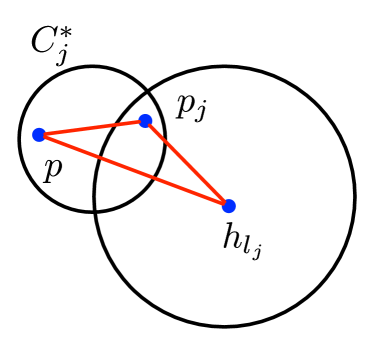
Figure 1: $||p-h_{l_{j}}||\leq||p-p_{j}||+||p_{j}-h_{l_{j}}||\leq 4r_{\mathtt{opt}}$.

See Figure 1 for an illustration. Overall, $P_{\mathtt{opt}}=\cup^{k}_{j=1}C^{*}_{j}$ is covered by the union of the balls $\cup^{k+k^{\prime}}_{l=1}\texttt{Ball}(h_{l},4r_{\mathtt{opt}})$, i.e., $\Delta^{-z}_{\infty}(P,H)\leq 4r_{\mathtt{opt}}$. ∎

An “extreme” example for Theorem 1. We present an example to show that the value of $k^{\prime}$ in Step 2 cannot be reduced. Namely, the clustering quality could be arbitrarily bad if we run $(k+k^{\prime\prime})$-center clustering on $S$ with $k^{\prime\prime}<k^{\prime}$. Let $P$ be an $(\epsilon_{1},\epsilon_{2})$-significant instance in $\mathbb{R}^{d}$, where each optimal cluster $C^{*}_{j}$ is a set of $|C^{*}_{j}|$ overlapping points located at its cluster center $o^{*}_{j}$. Let $x>0$ and $y\gg x$. We assume (1) $||o^{*}_{j_{1}}-o^{*}_{j_{2}}||=x$, $\forall j_{1}\neq j_{2}$; (2) $||q_{1}-q_{2}||\geq y$, $\forall q_{1},q_{2}\in P\setminus P_{\mathtt{opt}}$; (3) $||o^{*}_{j}-q||\geq y$, $\forall 1\leq j\leq k,q\in P\setminus P_{\mathtt{opt}}$. Obviously, the optimal radius $r_{\mathtt{opt}}=0$. Suppose we obtain a sample $S$ satisfying $S\cap C^{*}_{j}\neq\emptyset$ for any $1\leq j\leq k$ and $|S\setminus P_{\mathtt{opt}}|=\frac{1}{\eta}\frac{\epsilon_{2}}{k}|S|=k^{\prime}$. Given a number $k^{\prime\prime}<k^{\prime}$, we run $(k+k^{\prime\prime})$-center clustering on $S$. Since the points of $S$ take $k+k^{\prime}$ distinct locations in the space, any $(k+k^{\prime\prime})$-center clustering on $S$ will yield a radius at least $x/2>0$ (because $y\gg x$, it forces to select the points from $S\setminus P_{\mathtt{opt}}$ as the cluster centers, and therefore there must exist two points of $S\cap P_{\mathtt{opt}}$ falling into one cluster); thus the approximation ratio is at least $\frac{x/2}{0}=+\infty$.

2.2 The Second Algorithm

We present the second algorithm (Algorithm 2) and analyze its quality in this section.

Theorem 2.

If $\frac{\epsilon_{1}}{\epsilon_{2}}>\frac{1}{\eta(1-\delta)}$, with probability at least $(1-\eta)^{2}$, Algorithm 2 returns $k$ cluster centers that achieve a $(c+2)$-approximation for $k$-center clustering with $z$ outliers, i.e., $\Delta^{-z}_{\infty}(P,H)\leq(c+2)r_{\mathtt{opt}}$.

Remark 5.

As an example, if we set $\eta=\delta=1/2$, the algorithm works for any instance with $\frac{\epsilon_{1}}{\epsilon_{2}}>\frac{1}{\eta(1-\delta)}=4$. Actually, as long as $\frac{\epsilon_{1}}{\epsilon_{2}}>1$ (i.e., $\min_{1\leq j\leq k}|C^{*}_{j}|>z$), we can always find the appropriate values for $\eta$ and $\delta$ to satisfy $\frac{\epsilon_{1}}{\epsilon_{2}}>\frac{1}{\eta(1-\delta)}$, e.g., we can set $\eta=\sqrt{\frac{\epsilon_{2}}{\epsilon_{1}}}$ and $\delta<1-\sqrt{\frac{\epsilon_{2}}{\epsilon_{1}}}$. Obviously, if $\frac{\epsilon_{1}}{\epsilon_{2}}$ is close to $1$, the success probability $(1-\eta)^{2}$ could be small. To boost the success probability, we repeat the algorithm multiple times and select the best one in our experiments of Section 4. By repeatedly running the algorithm, we can achieve a constant success probability, as stated in Corollary 1. This also implies an important observation: the larger the ratio $\frac{\epsilon_{1}}{\epsilon_{2}}$ is , the more effectively uniform sampling performs.

Corollary 1.

By executing Algorithm 1 $O(\frac{1}{(1-\eta)^{2}})$ times, with constant probability, there exists at least one time where the returned $k$ centers $H$ satisfy $\Delta^{-z}_{\infty}(P,H)\leq(c+2)r_{\mathtt{opt}}$.

Proof.

(of Theorem 2) Similar to the proof of Theorem 1, we assume that $|S\cap C^{*}_{j}|\in(1\pm\delta)\frac{|C^{*}_{j}|}{n}|S|$ for each $C^{*}_{j}$, and $S$ has at most $\hat{z}=\frac{\epsilon_{2}}{k\eta}|S|$ points from $P\setminus P_{\mathtt{opt}}$. Let $\mathbb{B}_{S}=\{\texttt{Ball}(h_{l},r)\mid 1\leq l\leq k\}$ be the set of $k$ balls returned in Step 2 of Algorithm 2. Since $S\cap P_{\mathtt{opt}}$ can be covered by $k$ balls with radius $r_{\mathtt{opt}}$ and $|S\setminus P_{\mathtt{opt}}|\leq\hat{z}$, the optimal radius for the instance $S$ with $\hat{z}$ outliers should be at most $r_{\mathtt{opt}}$. Consequently, $r\leq cr_{\mathtt{opt}}$. Moreover, we have

$$|S\cap C^{*}_{j}| \geq (1-\delta)\frac{|C^{*}_{j}|}{n}|S|$$ (3)

$$\geq (1-\delta)\frac{\epsilon_{1}}{k}|S|$$

$$> (1-\delta)\frac{\epsilon_{2}}{\eta(1-\delta)k}|S|$$

$$= \frac{\epsilon_{2}}{\eta k}|S|=\hat{z}$$

for any $1\leq j\leq k$, where the last inequality comes from the assumption $\frac{\epsilon_{1}}{\epsilon_{2}}>\frac{1}{\eta(1-\delta)}$. Thus, if we perform $k$-center clustering with $\hat{z}$ outliers on $S$, the obtained $k$ balls must cover at least one point from each $C^{*}_{j}$ (since $|S\cap C^{*}_{j}|>\hat{z}$ from (3)). Through a similar manner in the proof of Theorem 1, we know that $P_{\mathtt{opt}}=\cup^{k}_{j=1}C^{*}_{j}$ is covered by the union of the balls $\cup^{k}_{l=1}\texttt{Ball}(h_{l},r+2r_{\mathtt{opt}})$, i.e.,

$$\Delta^{-z}_{\infty}(P,H)\leq r+2r_{\mathtt{opt}}\leq(c+2)r_{\mathtt{opt}}.$$ (4)

∎

Runtime: Similar to Algorithm 1, the sample size $|S|=\frac{3k}{\delta^{2}\epsilon_{1}}\log\frac{2k}{\eta}$ depends on $k$, $\epsilon_{1}$, and the parameters $\delta$ and $\eta$ only. The runtime depends on the complexity of the subroutine $c$-approximation algorithm used in Step 2. For example, the algorithm of Charikar et al. [9] takes $O\big{(}|S|^{2}d+k|S|^{2}\log|S|\big{)}$ time in $\mathbb{R}^{d}$.

Algorithm 2 Uni-$k$-Center Outliers ii@

  Input: An $(\epsilon_{1},\epsilon_{2})$-significant instance $P$ of $k$-center clustering with $z$ outliers, and $|P|=n$; two parameters $\eta,\delta\in(0,1)$.

  

1. Sample a set $S$ of $\frac{3k}{\delta^{2}\epsilon_{1}}\log\frac{2k}{\eta}$ points uniformly at random from $P$.

2. Let $\hat{z}=\frac{1}{\eta}\frac{\epsilon_{2}}{k}|S|$, and solve the $k$-center clustering with $\hat{z}$ outliers problem on $S$ by using any $c$-approximation algorithm with $c\geq 1$ (e.g., the $3$-approximation algorithm [9]).

  Output $H$, which is the set of $k$ cluster centers returned in Step 2.

3 $k$-Median/Means clustering with outliers

For $k$-means clustering with outliers, we apply the similar uniform sampling ideas as Algorithm 1 and 2. However, the analyses are more complicated here. For ease of understanding, we present our high-level idea first. Also, we provide the extensions for $k$-median clustering with outliers and their counterparts in arbitrary metric space in appendix.

High-level idea. Recall $\{C^{*}_{1},C^{*}_{2},\cdots,C^{*}_{k}\}$ are the $k$ optimal clusters. Denote by $O^{*}=\{o^{*}_{1},\cdots,o^{*}_{k}\}$ the mean points of $\{C^{*}_{1},\cdots,C^{*}_{k}\}$, respectively. We define the following transformation on $P_{\mathtt{opt}}$ to help us analyzing the clustering errors. For each point in $C^{*}_{j}$, we translate it to $o^{*}_{j}$; overall, we generate a new set of $n-z$ points located at $\{o^{*}_{1},\cdots o^{*}_{k}\}$, where each $o^{*}_{j}$ has $|C^{*}_{j}|$ overlapping points. (1) For any point $p\in C^{*}_{j}$ with $1\leq j\leq k$, denote by $\tilde{p}$ its transformed point. (2) For any $U\subseteq P_{\mathtt{opt}}$, denote by $\tilde{U}$ its transformed point set. Since the transformation forms $k$ “stars” (see Figure 2), we call it “star shaped transformation”.

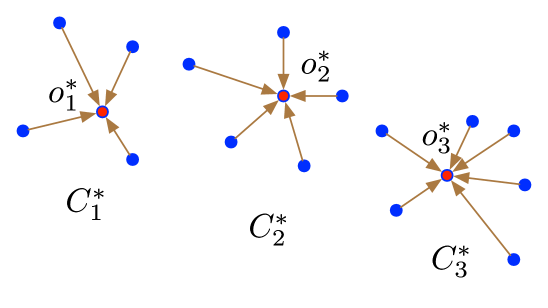
Figure 2: The transformation from $P_{\mathtt{opt}}$ to $\tilde{P}_{\mathtt{opt}}$.

Let $S$ be a sufficiently large random sample from $P$. We first show that $S\cap C^{*}_{j}$ can well approximate $C^{*}_{j}$ for each $1\leq j\leq k$. Informally,

$$\left.\begin{aligned} \frac{|S\cap C^{*}_{j}|}{|S|}&\approx\frac{|C^{*}_{j}|}{n};\\ \frac{1}{|S\!\cap\!C^{*}_{j}|}\sum_{q\in S\cap C^{*}_{j}}||q\!-\!o^{*}_{j}||^{2}&\approx\frac{1}{|C^{*}_{j}|}\sum_{p\in C^{*}_{j}}||p\!-\!o^{*}_{j}||^{2}.\end{aligned}\right\}$$ (5)

Let $S_{\mathtt{opt}}=S\cap P_{\mathtt{opt}}$. By using (5), we can prove that the clustering costs of $\tilde{P}_{\mathtt{opt}}$ and $\tilde{S}_{\mathtt{opt}}$ are close (after the normalization) for any given set of cluster centers in the Euclidean space. Similar to Algorithm 1, we compute the $(k+k^{\prime})$-means clustering on the sample $S$ in Algorithm 3, where $k^{\prime}$ is roughly $O(\frac{\log k}{\xi^{2}})$ with a parameter $\xi\in(0,1)$. Let $H$ be the returned set of $k+k^{\prime}$ cluster centers. Then, we can use $\tilde{S}_{\mathtt{opt}}$ and $\tilde{P}_{\mathtt{opt}}$ as the “bridges” to connect $S$ and $P$, so as to prove the theoretical quality guarantee of Algorithm 3.

In the second algorithm (similar to Algorithm 2), we run a $k$-means with $\hat{z}$ outliers algorithm on the sample $S$ and return exactly $k$ (rather than $k+k^{\prime}$) cluster centers. Let $S_{\mathtt{in}}$ be the set of obtained $|S|-\hat{z}$ inliers of $S$. If $\frac{\epsilon_{1}}{\epsilon_{2}}>1$, we can prove that $|S_{\mathtt{in}}\cap C^{*}_{j}|\approx|S\cap C^{*}_{j}|$ for each $1\leq j\leq k$. Therefore, we can replace “$S$” by “$S_{\mathtt{in}}$” in (5) and prove a similar quality guarantee.

We present Algorithm 3 and Algorithm 4 to realize the above ideas, and provide the main theorems below. In Theorem 3, $\mathcal{L}$ denotes the maximum diameter of the $k$ clusters $C^{*}_{1},\cdots,C^{*}_{k}$, i.e., $\mathcal{L}$$=\max_{1\leq j\leq k}\max_{p,q\in C^{*}_{j}}$ $||p-q||$. Actually, our result can be viewed as an extension of the sublinear time $k$-means clustering algorithms [40, 41] (who also have the additive clustering cost errors) to the case with outliers. We need to emphasize that the additive error is unavoidable even for the case without outliers, if we require the sample complexity to be independent of the input size [40, 41]. Though the $k$-median clustering with outliers algorithm in Meyerson et al. [17, Section 6] does not yield an additive error, as mentioned in Section 1, it needs to discard more than $16z$ outliers and the sample size depends on the ratio $n/z$.

Algorithm 3 Uni-$k$-Means Outliers i@

  Input: An $(\epsilon_{1},\epsilon_{2})$-significant instance $P$ of $k$-means clustering with $z$ outliers in $\mathbb{R}^{d}$, and $|P|=n$; three parameters $\eta,\delta,\xi\in(0,1)$.

  

1. Take a uniform sample $S$ of $\max\{\frac{3k}{\delta^{2}\epsilon_{1}}\log\frac{2k}{\eta},$ $\frac{k}{2\xi^{2}\epsilon_{1}(1-\delta)}\log\frac{2k}{\eta}\}$ points from $P$.

2. Let $k^{\prime}=\frac{1}{\eta}\frac{\epsilon_{2}}{k}|S|$, and solve the $(k+k^{\prime})$-means clustering on $S$ by using any $c$-approximation algorithm with $c\geq 1$.

  Output $H$, which is the set of $k+k^{\prime}$ cluster centers returned in Step 2.

Theorem 3.

Let $0<\delta,\eta,\xi<1$. With probability at least $(1-\eta)^{3}$, the set of cluster centers $H$ returned by Algorithm 3 yields a clustering cost $\Delta^{-z}_{2}(P,H)\leq\alpha\Delta^{-z}_{2}(P,O^{*})+\beta\xi\mathcal{L}^{2}$, where $\alpha=\big{(}2+(4+4c)\frac{1+\delta}{1-\delta}\big{)}$ and $\beta=(4+4c)\frac{1+\delta}{1-\delta}$.

Remark 6.

(i) In Step 2 of Algorithm 3, we can apply an $O(1)$-approximation $k$-means algorithm (e.g., [45]). If we assume $1/\delta$ and $1/\eta$ are fixed constants, then the sample size $|S|=O(\frac{k}{\xi^{2}\epsilon_{1}}\log k)$, and both the factors $\alpha$ and $\beta$ are $O(1)$, i.e.,

$$\Delta^{-z}_{2}(P,H)\leq O(1)\cdot\Delta^{-z}_{2}(P,O^{*})+O(\xi)\cdot\mathcal{L}^{2}.$$ (6)

The additive error $O(\xi)\cdot\mathcal{L}^{2}$ converges to $0$ when $\xi$ goes to $0$. Moreover, the number of returned cluster centers $|H|=k+O(\frac{\log k}{\xi^{2}})$ if $\frac{\epsilon_{1}}{\epsilon_{2}}=\Omega(1)$.

(ii) It is also easy to see that the extreme example proposed at the end of Section 2.1 also works for Algorithm 3, i.e., the value of $k^{\prime}$ cannot be reduced.

Before proving Theorem 3, we need to introduce the following lemmas.

Lemma 3.

We fix a cluster $C^{*}_{j}$. Given $\eta,\xi\in(0,1)$, if one uniformly selects a set $T$ of $\frac{1}{2\xi^{2}}\log\frac{2}{\eta}$ or more points at random from $C^{*}_{j}$, then

$$\bigg{|}\frac{1}{|T|}\sum_{q\in T}||q-o^{*}_{j}||^{2}-\frac{1}{|C^{*}_{j}|}\sum_{p\in C^{*}_{j}}||p-o^{*}_{j}||^{2}\bigg{|}\leq\xi\mathcal{L}^{2}$$ (7)

with probability at least $1-\eta$.

Lemma 3 can be obtained via the Hoeffding’s inequality (each $||q-o^{*}_{j}||^{2}$ can be viewed as a random variable between $0$ and $\mathcal{L}^{2}$) [44].

Lemma 4.

If one uniformly selects a set $S$ of $\max\{\frac{3k}{\delta^{2}\epsilon_{1}}\log\frac{2k}{\eta},$ $\frac{k}{2\xi^{2}\epsilon_{1}(1-\delta)}\log\frac{2k}{\eta}\}$ points at random from $P$, then

$$\sum_{q\in S\cap C^{*}_{j}} ||q-o^{*}_{j}||^{2}$$

$$\leq(1+\delta)\frac{|S|}{n}\big{(}\sum_{p\in C^{*}_{j}}||p-o^{*}_{j}||^{2}+\xi|C^{*}_{j}|\mathcal{L}^{2}\big{)}$$ (8)

for each $1\leq j\leq k$, with probability at least $(1-\eta)^{2}$.

Proof.

Suppose

$$|S|=\max\{\frac{3k}{\delta^{2}\epsilon_{1}}\log\frac{2k}{\eta},\frac{k}{2\xi^{2}\epsilon_{1}(1-\delta)}\log\frac{2k}{\eta}\}.$$

According to Lemma 1, $|S|\geq\frac{3k}{\delta^{2}\epsilon_{1}}\log\frac{2k}{\eta}$ implies

$$|S\cap C^{*}_{j}|\geq(1-\delta)\frac{|C^{*}_{j}|}{n}|S|\geq(1-\delta)\frac{\epsilon_{1}}{k}|S|$$ (9)

for each $1\leq j\leq k$, with probability at least $1-\eta$. Below, we assume (9) occurs. Further, $|S|\geq\frac{k}{2\xi^{2}\epsilon_{1}(1-\delta)}\log\frac{2k}{\eta}$ implies

$$(1-\delta)\frac{\epsilon_{1}}{k}|S|\geq\frac{1}{2\xi^{2}}\log\frac{2k}{\eta}.$$ (10)

Combining (9) and (10), we have $|S\cap C^{*}_{j}|\geq\frac{1}{2\xi^{2}}\log\frac{2k}{\eta}$. Consequently, through Lemma 3 we obtain

$$\bigg{|}\frac{1}{|S\cap C^{*}_{j}|}\sum_{q\in S\cap C^{*}_{j}}||q-o^{*}_{j}||^{2}-\frac{1}{|C^{*}_{j}|}\sum_{p\in C^{*}_{j}}||p-o^{*}_{j}||^{2}\bigg{|}\leq\xi\mathcal{L}^{2}$$ (11)

for each $1\leq j\leq k$, with probability at least $1-\eta$ ($\eta$ is replaced by $\eta/k$ in Lemma 3 for taking the union bound). From (11) we have

$$\sum_{q\in S\cap C^{*}_{j}}||q-o^{*}_{j}||^{2}\leq|S\cap C^{*}_{j}|\big{(}\frac{1}{|C^{*}_{j}|}\sum_{p\in C^{*}_{j}}||p-o^{*}_{j}||^{2}+\xi\mathcal{L}^{2}\big{)}$$

$$\leq(1+\delta)\frac{|C^{*}_{j}|}{n}|S|\big{(}\frac{1}{|C^{*}_{j}|}\sum_{p\in C^{*}_{j}}||p-o^{*}_{j}||^{2}+\xi\mathcal{L}^{2}\big{)}$$

$$=(1+\delta)\frac{|S|}{n}\big{(}\sum_{p\in C^{*}_{j}}||p-o^{*}_{j}||^{2}+\xi|C^{*}_{j}|\mathcal{L}^{2}\big{)},$$ (12)

where the second inequality comes from Lemma 1. The overall success probability $(1-\eta)^{2}$ comes from the success probabilities of (9) and (11). So we complete the proof. ∎

For ease of presentation, we define a new notation that is used in the following lemmas. Given two point sets $X$ and $Y\subset\mathbb{R}^{d}$, we use $\texttt{\bf{Cost}}(X,Y)$ to denote the clustering cost of $X$ by taking $Y$ as the cluster centers, i.e., $\texttt{\bf{Cost}}(X,Y)=\sum_{q\in X}(\texttt{dist}(q,Y))^{2}$. Obviously, $\Delta^{-z}_{2}(P,H)=\frac{1}{n-z}\texttt{\bf{Cost}}(P_{\mathtt{opt}},H)$. Let $S_{\mathtt{opt}}=S\cap P_{\mathtt{opt}}$. Below, we prove the upper bounds of $\texttt{\bf{Cost}}(S_{\mathtt{opt}},O^{*})$, $\texttt{\bf{Cost}}(\tilde{S}_{\mathtt{opt}},H)$, and $\texttt{\bf{Cost}}(\tilde{P}_{\mathtt{opt}},H)$ respectively, and use these bounds to complete the proof of Theorem 3. For convenience, we always assume that the events described in Lemma 1, Lemma 2, and Lemma 4 all occur, so that we do not need to repeatedly state the success probabilities.

Lemma 5.

$\texttt{\bf{Cost}}(S_{\mathtt{opt}},O^{*})\leq(1+\delta)\frac{|S|}{n}(n-z)\big{(}\Delta^{-z}_{2}(P,O^{*})+\xi\mathcal{L}^{2}\big{)}$.

Proof.

First, we have

Cost $$(S_{\mathtt{opt}},O^{*})\!=\!\sum^{k}_{j=1}\sum_{q\in S\cap C^{*}_{j}}||q-o^{*}_{j}||^{2}$$

$$\!\leq\!(1\!+\!\delta)\frac{|S|}{n}\sum^{k}_{j=1}\big{(}\sum_{p\in C^{*}_{j}}||p-o^{*}_{j}||^{2}\!+\!\xi|C^{*}_{j}|\mathcal{L}^{2}\big{)}$$ (13)

by Lemma 4. Further, since $\sum^{k}_{j=1}\sum_{p\in C^{*}_{j}}||p-o^{*}_{j}||^{2}=(n-z)\Delta^{-z}_{2}(P,O^{*})$ and $\sum^{k}_{j=1}|C^{*}_{j}|=n-z$, by plugging them into (13), we obtain Lemma 5. ∎

Lemma 6.

$\texttt{\bf{Cost}}(\tilde{S}_{\mathtt{opt}},H)\leq(2+2c)\cdot\texttt{\bf{Cost}}(S_{\mathtt{opt}},O^{*})$.

Proof.

We fix a point $q\in S_{\mathtt{opt}}$, and assume that the nearest neighbors of $q$ and $\tilde{q}$ in $H$ are $h_{j_{q}}$ and $h_{\tilde{j}_{q}}$, respectively. Then, we have

$$||\tilde{q}-h_{\tilde{j}_{q}}||^{2} \leq||\tilde{q}-h_{j_{q}}||^{2}$$

$$\leq 2||\tilde{q}-q||^{2}+2||q-h_{j_{q}}||^{2}.$$ (14)

Therefore,

$$\sum_{q\in S_{\mathtt{opt}}}||\tilde{q}\!-\!h_{\tilde{j}_{q}}||^{2} \!\leq\!2\!\sum_{q\in S_{\mathtt{opt}}}||\tilde{q}\!-\!q||^{2}\!+\!2\!\sum_{q\in S_{\mathtt{opt}}}||q\!-\!h_{j_{q}}||^{2},$$

$$\implies\texttt{\bf{Cost}}(\tilde{S}_{\mathtt{opt}},H) \leq 2\texttt{\bf{Cost}}(S_{\mathtt{opt}},O^{*})+2\texttt{\bf{Cost}}(S_{\mathtt{opt}},H).$$ (15)

Moreover, since $S_{\mathtt{opt}}\subseteq S$ (because $S_{\mathtt{opt}}=S\cap P_{\mathtt{opt}}$) and $H$ yields a $c$-approximate clustering cost of the $(k+k^{\prime})$-means clustering on $S$, we have

$$\texttt{\bf{Cost}}(S_{\mathtt{opt}},H)\leq\texttt{\bf{Cost}}(S,H)\leq c\cdot W,$$ (16)

where $W$ is the optimal clustering cost of $(k+k^{\prime})$-means clustering on $S$. Let $S^{\prime}$ be the $k^{\prime}$ farthest points of $S$ to $O^{*}$, then the set $O^{*}\cup S^{\prime}$ also forms a solution for $(k+k^{\prime})$-means clustering on $S$; namely, $S$ is partitioned into $k+k^{\prime}$ clusters where each point of $S^{\prime}$ is a cluster having a single point. Obviously, such a clustering yields a clustering cost $(|S|-k^{\prime})\Delta^{-k^{\prime}}_{2}(S,O^{*})$. Consequently,

$$W\leq(|S|-k^{\prime})\Delta^{-k^{\prime}}_{2}(S,O^{*}).$$ (17)

Also, Lemma 2 shows that $S$ contains at most $k^{\prime}$ points from $P\setminus P_{\mathtt{opt}}$, i.e., $|S_{\mathtt{opt}}|\geq|S|-k^{\prime}$. Thus,

$$\texttt{\bf{Cost}}(S_{\mathtt{opt}},O^{*})\geq(|S|-k^{\prime})\Delta^{-k^{\prime}}_{2}(S,O^{*}).$$ (18)

Together with (15), (16), and (17), we have $\texttt{\bf{Cost}}(\tilde{S}_{\mathtt{opt}},H)\leq(2+2c)\cdot\texttt{\bf{Cost}}(S_{\mathtt{opt}},O^{*})$. ∎

Lemma 7.

$\texttt{\bf{Cost}}(\tilde{P}_{\mathtt{opt}},H)\leq\frac{1}{1-\delta}\frac{n}{|S|}\texttt{\bf{Cost}}(\tilde{S}_{\mathtt{opt}},H)$.

Proof.

From the constructions of $\tilde{P}_{\mathtt{opt}}$ and $\tilde{S}_{\mathtt{opt}}$, we know that they are overlapping points locating at $\{o^{*}_{1},\cdots,o^{*}_{k}\}$. From Lemma 1, we know $|S\cap C^{*}_{j}|\geq(1-\delta)\frac{|C^{*}_{j}|}{n}|S|$, i.e.,

$$|C^{*}_{j}|\leq\frac{1}{1-\delta}\frac{n}{|S|}|S\cap C^{*}_{j}|\text{ for $1\leq j\leq k$.}$$ (19)

Overall, we have $\texttt{\bf{Cost}}(\tilde{P}_{\mathtt{opt}},H)=\sum^{k}_{j=1}|C^{*}_{j}|\big{(}\texttt{dist}(o^{*}_{j},H)\big{)}^{2}$ that is at most

$$\frac{1}{1-\delta}\frac{n}{|S|}\sum^{k}_{j=1}|S\cap C^{*}_{j}|\big{(}\texttt{dist}(o^{*}_{j},H)\big{)}^{2}$$

$$=\frac{1}{1-\delta}\frac{n}{|S|}\texttt{\bf{Cost}}(\tilde{S}_{\mathtt{opt}},H).$$

∎

Now, we are ready to prove Theorem 3.

Proof.

(of Theorem 3) Note that $(n-z)\Delta^{-z}_{2}(P,H)$ actually is the $|H|$-means clustering cost of $P$ by removing the farthest $z$ points to $H$, and $|P_{\mathtt{opt}}|=n-z$. So we have

$$(n-z)\Delta^{-z}_{2}(P,H)\leq\texttt{\bf{Cost}}(P_{\mathtt{opt}},H).$$ (20)

Further, by using a similar manner of (15), we have $\texttt{\bf{Cost}}(P_{\mathtt{opt}},H)\leq 2\texttt{\bf{Cost}}(P_{\mathtt{opt}},O^{*})+2\texttt{\bf{Cost}}(\tilde{P}_{\mathtt{opt}},H)$. Therefore,

$$\Delta^{-z}_{2}(P,H)\leq\frac{1}{n-z}\texttt{\bf{Cost}}(P_{\mathtt{opt}},H)$$ (21)

$$\leq\frac{2}{n-z}\Big{(}\texttt{\bf{Cost}}(P_{\mathtt{opt}},O^{*})+\texttt{\bf{Cost}}(\tilde{P}_{\mathtt{opt}},H)\Big{)}.$$ (22)

Moreover,

$$\texttt{\bf{Cost}}(\tilde{P}_{\mathtt{opt}},H) \leq\frac{1}{1-\delta}\frac{n}{|S|}\texttt{\bf{Cost}}(\tilde{S}_{\mathtt{opt}},H)$$ (23)

$$\leq\frac{1}{1-\delta}\frac{n}{|S|}(2+2c)\texttt{\bf{Cost}}(S_{\mathtt{opt}},O^{*})$$ (24)

$$\leq\!\frac{1\!+\!\delta}{1\!-\!\delta}(2\!+\!2c)(n\!-\!z)\big{(}\Delta^{-z}_{2}(P,O^{*})\!+\!\xi\mathcal{L}^{2}\big{)},$$ (25)

where (23), (24), and (25) come from Lemma 7, Lemma 6, and Lemma 5 respectively. From the fact $\texttt{\bf{Cost}}(P_{\mathtt{opt}},O^{*})=(n-z)\Delta^{-z}_{2}(P,O^{*})$, (22) and (25) imply $\Delta^{-z}_{2}(P,H)\leq\big{(}2\!+\!(4\!+\!4c\!)\frac{1\!+\!\delta}{1\!-\!\delta}\big{)}\Delta^{-z}_{2}(P\!,\!O^{*})\!+\!(4\!+\!4c)\frac{1\!+\!\delta}{1\!-\!\delta}\xi\mathcal{L}^{2}$.

The success probability $(1-\eta)^{3}$ comes from Lemma 4 and Lemma 2 (note that Lemma 4 already takes into account of the success probability of Lemma 1 ). Thus, we complete the proof of Theorem 3. ∎

Algorithm 4 Uni-$k$-Means Outliers ii@

  Input: An $(\epsilon_{1},\epsilon_{2})$-significant instance $P$ of $k$-means clustering with $z$ outliers in $\mathbb{R}^{d}$, and $|P|=n$; three parameters $\eta,\delta,\xi\in(0,1)$.

  

1. Take a uniform sample $S$ of $\max\{\frac{3k}{\delta^{2}\epsilon_{1}}\log\frac{2k}{\eta},$ $\frac{k}{2\xi^{2}\epsilon_{1}(1-\delta)}\log\frac{2k}{\eta}\}$ points from $P$.

2. Let $\hat{z}=\frac{1}{\eta}\frac{\epsilon_{2}}{k}|S|$, and solve the $k$-means clustering with $\hat{z}$ outliers on $S$ by using any $c$-approximation algorithm with $c\geq 1$.

  Output $H$, which is the set of $k$ cluster centers returned in Step 2.

Theorem 4.

Let $0<\delta,\eta,\xi<1$, and $t=\eta(1-\delta)\frac{\epsilon_{1}}{\epsilon_{2}}$. Assume $t>1$. With probability at least $(1-\eta)^{3}$, the set of cluster centers $H$ returned by Algorithm 4 yields a clustering cost $\Delta^{-z}_{2}(P,H)\leq\alpha\Delta^{-z}_{2}(P,O^{*})+\beta\xi\mathcal{L}^{2}$, where $\alpha=\big{(}2+(4+4c)\frac{t}{t-1}\frac{1+\delta}{1-\delta}\big{)}$ and $\beta=(4+4c)\frac{t}{t-1}\frac{1+\delta}{1-\delta}$.

Remark 7.

Similar to Remark 5, as long as $\frac{\epsilon_{1}}{\epsilon_{2}}>1$, we can set $\eta=\sqrt{\frac{\epsilon_{2}}{\epsilon_{1}}}$ and $\delta<1-\sqrt{\frac{\epsilon_{2}}{\epsilon_{1}}}$ to keep $t>1$. Additionally, like Corollary 1, we can repeat the algorithm $\frac{1}{(1-\eta)^{3}}$ times to achieve a constant success probability. If $\frac{t}{t-1}=O(1)$ and $c=O(1)$, then the clustering cost of Theorem 4 will be

$$\Delta^{-z}_{2}(P,H)\leq O(1)\cdot\Delta^{-z}_{2}(P,O^{*})+O(\xi)\cdot\mathcal{L}^{2}.$$ (26)

Also, when $\frac{\epsilon_{1}}{\epsilon_{2}}$ is large, the success probability becomes high as well. This also agrees with our previous observation concluded in Remark 5, that is, the ratio $\frac{\epsilon_{1}}{\epsilon_{2}}$ is an important factor that affects the performance of the uniform sampling approach.

Before proving Theorem 4, we introduce the following lemmas first. Suppose the $k$ clusters of $S$ obtained in Step (2) of Algorithm 4 are $S_{1},S_{2},\cdots,S_{k}$, and thus the inliers $S_{\mathtt{in}}=\cup^{k}_{j=1}S_{j}$. Similar to the proof of Theorem 3, below we always assume that the events described in Lemma 1, Lemma 2, and Lemma 4 all occur, so that we do not need to repeatedly state the success probabilities.

Lemma 8.

$\frac{|C^{*}_{j}|}{|C^{*}_{j}\cap S_{\mathtt{in}}|}\leq\frac{n}{|S|}\frac{t}{(t-1)(1-\delta)}$ for each $1\leq j\leq k$.

Proof.

Since $\hat{z}=\frac{1}{\eta}\frac{\epsilon_{2}}{k}|S|$ and $|S\cap C^{*}_{j}|\geq(1-\delta)\frac{|C^{*}_{j}|}{n}|S|$ for each $1\leq j\leq k$ (by Lemma 1), we have

$$|S_{\mathtt{in}}\cap C^{*}_{j}| \geq|S\cap C^{*}_{j}|-\hat{z}\geq(1-\delta)\frac{|C^{*}_{j}|}{n}|S|-\frac{1}{\eta}\frac{\epsilon_{2}}{k}|S|$$

$$=\Big{(}1-\frac{1}{\eta(1-\delta)}\frac{\epsilon_{2}}{k}\frac{n}{|C^{*}_{j}|}\Big{)}(1-\delta)\frac{|C^{*}_{j}|}{n}|S|$$

$$\geq\Big{(}1-\frac{1}{\eta(1-\delta)}\frac{\epsilon_{2}}{\epsilon_{1}}\Big{)}(1-\delta)\frac{|C^{*}_{j}|}{n}|S|$$

$$=(1-\frac{1}{t})(1-\delta)\frac{|C^{*}_{j}|}{n}|S|,$$ (27)

where the last inequality comes from $|C^{*}_{j}|\geq\frac{\epsilon_{1}}{k}n$. Thus $\frac{|C^{*}_{j}|}{|C^{*}_{j}\cap S_{\mathtt{in}}|}\leq\frac{n}{|S|}\frac{t}{(t-1)(1-\delta)}$. ∎

Lemma 9.

$\texttt{\bf{Cost}}(S_{\mathtt{in}}\cap P_{\mathtt{opt}},H)\leq(1+\delta)\frac{|S|}{n}\cdot c\cdot\big{(}\texttt{\bf{Cost}}(P_{\mathtt{opt}},O^{*})+(n-z)\cdot\xi\mathcal{L}^{2}\big{)}$.

Proof.

Since $\hat{z}\geq|S\setminus P_{\mathtt{opt}}|=|S|-|S_{\mathtt{opt}}|$, i.e., $|S_{\mathtt{opt}}|\geq|S|-\hat{z}$, we have

$$(|S|-\hat{z})\Delta^{-\hat{z}}_{2}(S,O^{*}) \leq|S_{\mathtt{opt}}|\cdot\Delta^{-\hat{z}}_{2}(S,O^{*})$$

$$\leq\texttt{\bf{Cost}}(S_{\mathtt{opt}},O^{*})$$

$$\implies\Delta^{-\hat{z}}_{2}(S,O^{*}) \leq\frac{1}{|S|-\hat{z}}\texttt{\bf{Cost}}(S_{\mathtt{opt}},O^{*}),$$ (28)

where the second inequality is due to the same reason of (20). Because $H$ is a $c$-approximation on $S$,

$$\Delta^{-\hat{z}}_{2}(S,H) \leq c\cdot\Delta^{-\hat{z}}_{2}(S,O^{*})$$

$$\leq\frac{c}{|S|-\hat{z}}\texttt{\bf{Cost}}(S_{\mathtt{opt}},O^{*}),$$ (29)

where the second inequality comes from (28). Therefore,

$$\texttt{\bf{Cost}}(S_{\mathtt{in}}\cap P_{\mathtt{opt}},H)$$

$$\leq\texttt{\bf{Cost}}(S_{\mathtt{in}},H)=(|S|-\hat{z})\Delta^{-\hat{z}}_{2}(S,H)$$

$$\leq c\cdot\texttt{\bf{Cost}}(S_{\mathtt{opt}},O^{*})$$

$$\leq(1+\delta)\frac{|S|}{n}\cdot c\cdot(n-z)\big{(}\Delta^{-z}_{2}(P,O^{*})+\xi\mathcal{L}^{2}\big{)}$$

$$=(1\!+\!\delta)\frac{|S|}{n}\!\cdot\!c\!\cdot\!\big{(}\texttt{\bf{Cost}}(P_{\mathtt{opt}},\!O^{*})\!+\!(n\!-\!z)\!\cdot\!\xi\mathcal{L}^{2}\big{)},$$ (30)

where the second and third inequalities comes from (29) and Lemma 5, respectively. So we complete the proof. ∎

Since $S_{\mathtt{in}}\cap P_{\mathtt{opt}}\subseteq S_{\mathtt{opt}}$, we immediately have the following lemma via Lemma 5.

Lemma 10.

$\texttt{\bf{Cost}}(S_{\mathtt{in}}\cap P_{\mathtt{opt}},O^{*})\leq(1+\delta)\frac{|S|}{n}(n-z)\big{(}\Delta^{-z}_{2}(P,O^{*})+\xi\mathcal{L}^{2}\big{)}$.

Now, we are ready to prove Theorem 4.

Proof.

(of Theorem 4) For convenience, let $S^{\prime}_{\mathtt{in}}=S_{\mathtt{in}}\cap P_{\mathtt{opt}}$. Using the same manner of (15), we have

$$\texttt{\bf{Cost}}(\tilde{S}^{\prime}_{\mathtt{in}},H) \leq 2\texttt{\bf{Cost}}(S^{\prime}_{\mathtt{in}},O^{*})+2\texttt{\bf{Cost}}(S^{\prime}_{\mathtt{in}},H);$$ (31)

$$\texttt{\bf{Cost}}(P_{\mathtt{opt}},H) \leq 2\texttt{\bf{Cost}}(P_{\mathtt{opt}},O^{*})+2\texttt{\bf{Cost}}(\tilde{P}_{\mathtt{opt}},H).$$ (32)

Also, because $\texttt{\bf{Cost}}\!(\tilde{P}_{\mathtt{opt}},\!H)=\sum^{k}_{j=1}|C^{*}_{j}|(\texttt{dist}(o^{*}_{j},\!H))^{2}$ and $\texttt{\bf{Cost}}(\tilde{S}^{\prime}_{\mathtt{in}},H)$ $=\sum^{k}_{j=1}|C^{*}_{j}\cap S_{\mathtt{in}}|(\texttt{dist}(o^{*}_{j},H))^{2}$, we have

$$\frac{\texttt{\bf{Cost}}(\tilde{P}_{\mathtt{opt}},H)}{\texttt{\bf{Cost}}(\tilde{S}^{\prime}_{\mathtt{in}},H)}\leq\max_{1\leq j\leq k}\frac{|C^{*}_{j}|}{|C^{*}_{j}\cap S_{\mathtt{in}}|}.$$ (33)

As a consequence,

$$\texttt{\bf{Cost}}(\tilde{P}_{\mathtt{opt}},H) \leq\max_{1\leq j\leq k}\frac{|C^{*}_{j}|}{|C^{*}_{j}\cap S_{\mathtt{in}}|}\cdot\texttt{\bf{Cost}}(\tilde{S}^{\prime}_{\mathtt{in}},H)$$

$$\leq\frac{n}{|S|}\frac{t}{(t-1)(1-\delta)}\cdot\texttt{\bf{Cost}}(\tilde{S}^{\prime}_{\mathtt{in}},H)$$ (34)

where the last inequality comes from Lemma 8. From (31), (32), and (34), we have

$$\texttt{\bf{Cost}}(P_{\mathtt{opt}},H) \leq 2\texttt{\bf{Cost}}(P_{\mathtt{opt}},O^{*})+\frac{4n}{|S|}\frac{t}{(t-1)(1-\delta)}\cdot$$

$$\big{(}\texttt{\bf{Cost}}(S^{\prime}_{\mathtt{in}},O^{*})+\texttt{\bf{Cost}}(S^{\prime}_{\mathtt{in}},H)\big{)}.\!\!$$ (35)

By plugging the inequalities of Lemma 9 and Lemma 10 into (35), we can obtain Theorem 4. ∎

4 Experiments

All the experiments were conducted on a Ubuntu workstation with 2.40GHz Intel(R) Xeon(R) CPU E5-2680 and 256GB main memory. The algorithms were implemented in Matlab R2020b, and our code is available at https://github.com/h305142/lightweight-clustering

Algorithms for testing. We use several baseline algorithms mentioned in Section 1.1. For $k$-center clustering with outliers, we consider the $3$-approximation Charikar [9], the $(4+\epsilon)$-approximation MK [21], the $13$-approximation Malkomes [46], and the non-uniform sampling algorithms BVX [12] and DYW [19]. In our Algorithm 2, we apply MK as the black-box algorithm in Step 2 (though Charikar has a lower approximation ratio, we observe that MK runs faster and often achieves comparable clustering results in practice).

For $k$-means/median clustering with outliers, we consider the heuristic algorithm $k$-means$--$ [30] and three non-uniform sampling methods: the local search algorithm LocalSearch [10] (we use the fast implementation [47] for its $k$-means++ seeding), the data summary based algorithm DataSummary [14], and the recently proposed hybrid sampling algorithm Hybrid [11]. In our Algorithm 3 and Algorithm 4, we apply the $k$-means++ [47] and $k$-means$--$ respectively as the black-box algorithms in their Step 2.

Datasets. We generate the synthetic datasets in $\mathbb{R}^{100}$, where the points of each cluster follow a random Gaussian distribution (similar with the methods in Chen et al. [14], Im et al. [11]). For each synthetic dataset, we uniformly generate $z$ outliers at random outside the minimum enclosing balls of the obtained $k$ clusters.

We also choose $4$ real datasets from UCI machine learning repository [48]. (1) Covertype has $7$ clusters with $5.8\times 10^{5}$ points in $\mathbb{R}^{54}$; (2) Kddcup has $23$ clusters with $4.9\times 10^{6}$ points in $\mathbb{R}^{38}$; (3) Poking Hand has $10$ clusters with $10^{6}$ points in $\mathbb{R}^{10}$; (4) Shuttle has $7$ clusters with $5.8\times 10^{4}$ points in $\mathbb{R}^{9}$. We add $1\%$ outliers uniformly at random outside the enclosing balls of the clusters as we did for the synthetic datasets.

Some implementation details. When implementing our proposed algorithms (Algorithm 1-4), it is not quite convenient to set the values for the parameters $\{\eta,\xi,\delta\}$ in practice. In fact, we only need to determine the sample size $|S|$ and $k^{\prime}$ for running Algorithm 1 and Algorithm 3 (and similarly, $|S|$ and $\hat{z}$ for running Algorithm 2 and Algorithm 4). As an example, for Algorithm 1, it is sufficient to input $|S|$ and $k^{\prime}$ only, since we just need to compute the $(k+k^{\prime})$-center clustering on the sample $S$; moreover, it is more intuitive to directly set $|S|$ and $k^{\prime}$ rather than to set the parameters $\{\eta,\xi,\delta\}$. Therefore, we will conduct the experiments to observe the trends when varying the values $|S|$, $k^{\prime}$, and $\hat{z}$.

Another practical issue for implementation is the success probability. For Algorithm 2 and 4, when $\frac{\epsilon_{1}}{\epsilon_{2}}$ is close to $1$, the success probability could be low (as discussed in Remark 5). We can run the algorithm multiple times, and at least one time the algorithm will return a qualified solution with a higher probability (by simply taking the union bound). For example, if $\eta=0.8$ and we run Algorithm 2 $50$ times, the success probability will be $1-(1-(1-0.8)^{2})^{50}\approx 87\%$. Suppose we run the algorithm $m>1$ times and let $H_{1},\cdots,H_{m}$ be the set of output candidates. The remaining issue is that how to select the one that achieves the smallest objective value among all the candidates. We directly scan the whole dataset in one pass. When reading a point $p$ from $P$, we calculate its distance to all the candidates, i.e., $\mathtt{dist}(p,H_{1}),\cdots,\mathtt{dist}(p,H_{m})$; after scanning the whole dataset, we have calculated the clustering costs $\Delta^{-z}_{\infty}(P,H_{l})$ (resp., $\Delta^{-z}_{1}(P,H_{l})$ and $\Delta^{-z}_{2}(P,H_{l})$) for $1\leq l\leq m$ and then return the best one. Another benefit of this operation is that we can determine the clustering assignments for the data points simultaneously. When calculating $\mathtt{dist}(p,H_{l})$ for $1\leq l\leq m$, we record the index of its nearest cluster center in $H_{l}$; finally, we can return its corresponding clustering assignment in the selected best candidate.

Experimental design. Our experiments include three parts. (1) We fix the sample size $|S|$ to be $5\times 10^{-3}n$, and study the clustering quality (such as clustering cost, precision, and purity) and the running time. (2) We study the scalabilities of the algorithms with enlarging the data size $n$, and the stabilities of our proposed algorithms with varying the sampling ratio $|S|/n$. (3) Finally, we focus on other factors that may affect the practical performances.

4.1 Clustering Quality and Running Time

In this part, we fix the sample size $|S|$ to be $5\times 10^{-3}n$. For the synthetic datasets, we first set $n=10^{5}$, $k=8$, and $z=2\%n$. For Algorithm 1 and 3, the value $k^{\prime}$ should be $\frac{1}{\eta}\frac{\epsilon_{2}}{k}|S|$ which could be large (though it is only $O(\log k)$ in the asymptotic analysis). Although we have constructed the example in Section 2.1 to show that $k^{\prime}$ cannot be reduced in the worst case, we do not strictly follow this theoretical value in our experiments. Instead, we keep the ratio $\tau=\frac{k+k^{\prime}}{k}$ to be $1,\frac{4}{3},\frac{5}{3}$, and $2$ (i.e., run the black-box algorithms from Gonzalez [24], Arthur and Vassilvitskii [34] $\tau k$ steps). For Algorithm 2 and Algorithm 4, we set $\hat{z}=2\frac{\epsilon_{2}}{k}|S|$; as discussed for the implementation details before, to boost the success probability we run Algorithm 2 (resp., Algorithm 4) $10$ times and select the best candidate (as one trial); we count the total time of the $10$ runs for one trial. For each instance, we take $20$ trials and report the average results in Figure 3.

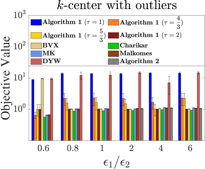
(a) Synthetic Datasets

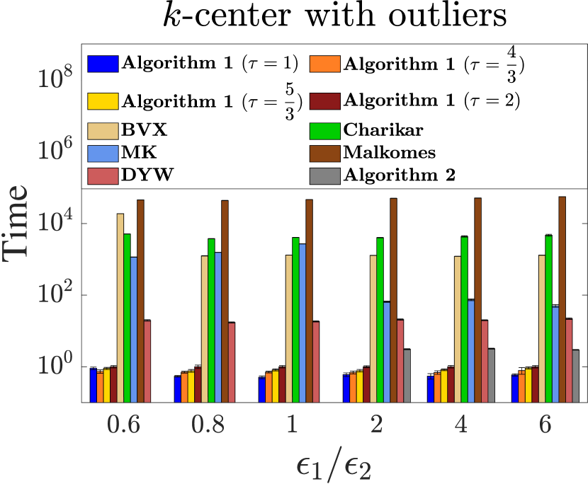
(b) Synthetic Datasets

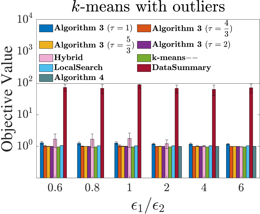
(c) Synthetic Datasets

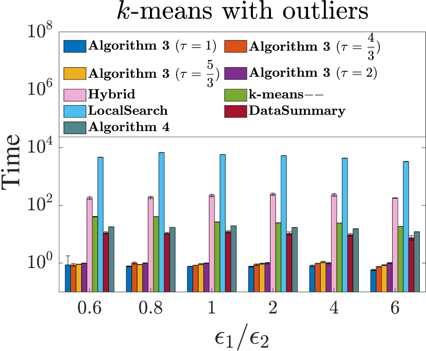
(d) Synthetic Datasets

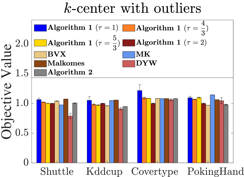
(e) Real Datasets

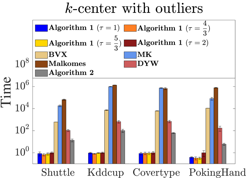
(f) Real Datasets

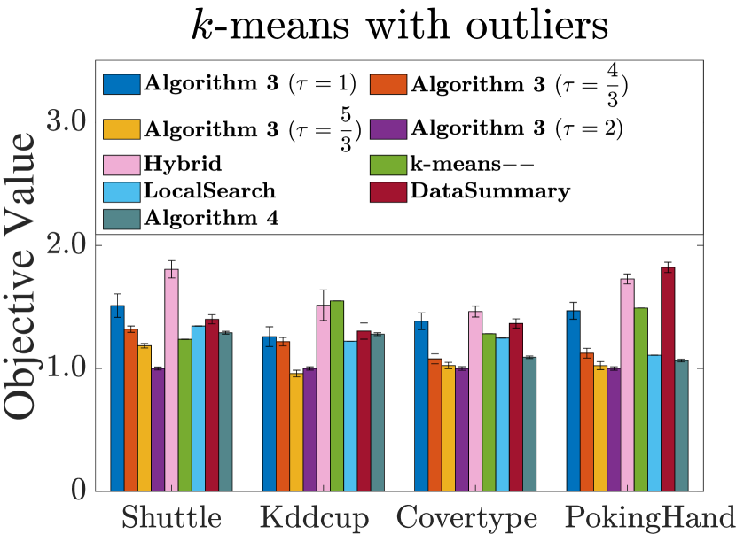
(g) Real Datasets

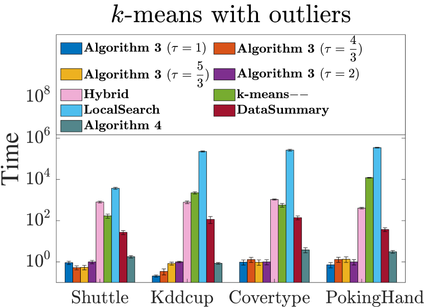
(h) Real Datasets

Figure 3: The normalized results (objective values and running times) for $k$-center and $k$-means clustering with outliers in synthetic data (Figure 3(a) $\sim$  3(d)) and real data (Figure 3(e) $\sim$  3(h)). To illustrate the comparisons more clearly, we normalize all the results by dividing them over the results of Algorithm 1 with $\tau=2$ (resp., Algorithm 3 with $\tau=2$ ) for $k$-center (resp., $k$-means/median ) clustering with outliers.

For $k$-center clustering with outliers, our algorithms (Algorithm 1 with $\tau\geq 4/3$ and Algorithm 2) and the four baseline algorithms achieve similar objective values for most of the instances (we run Algorithm 2 on the synthetic datasets with $\frac{\epsilon_{1}}{\epsilon_{2}}>1$ only; we do not run Charikar on the real datasets due to its high complexity). For $k$-means clustering with outliers, Algorithm 3 with $\tau\geq 4/3$ and Algorithm 4 can achieve the results close to the best of the three baseline algorithms. Moreover, the running times of our algorithms are significantly lower comparing with the baseline algorithms. Overall, we conclude that (1) Algorithm 1 and Algorithm 3 just need to return slightly more than $k$ cluster centers (e.g., $\frac{4}{3}k$) for achieving low clustering cost; (2) Algorithm 2 and Algorithm 4 can achieve low clustering cost when $\frac{\epsilon_{1}}{\epsilon_{2}}\geq 2$.

To further evaluate their clustering qualities, we consider the measures precision and purity, which have been widely used before [49]; these two measures both aim to evaluate the difference between the obtained clusters and the ground truth. (1) The precision is the proportion of the ground-truth outliers found by the algorithm (i.e., $\frac{|Out\cap Out_{\mathtt{truth}}|}{|Out_{\mathtt{truth}}|}$, where $Out$ is the set of returned outliers and $Out_{\mathtt{truth}}$ is the set of ground-truth outliers). (2) For each obtained cluster, we assign it to the ground-truth cluster which is most frequent in the obtained cluster, and the purity measures the accuracy of this assignment. Specifically, let $\{C_{1},C_{2},\cdots,C_{k}\}$ be the ground-truth clusters and $\{C^{\prime}_{1},C^{\prime}_{2},\cdots,C^{\prime}_{k}\}$ be the obtained clusters from the algorithm; the purity is equal to $\frac{1}{n-z}\sum^{k}_{j=1}\max_{1\leq l\leq k}|C^{\prime}_{j}\cap C_{l}|$. In general, the precisions and the purities achieved by our uniform sampling approaches and the baseline algorithms are relatively close. The numerical results are shown in Table 1 and 2.

4.2 Scalability and Sampling Ratio

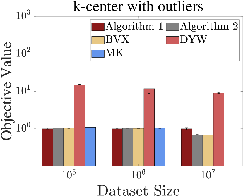
(a)

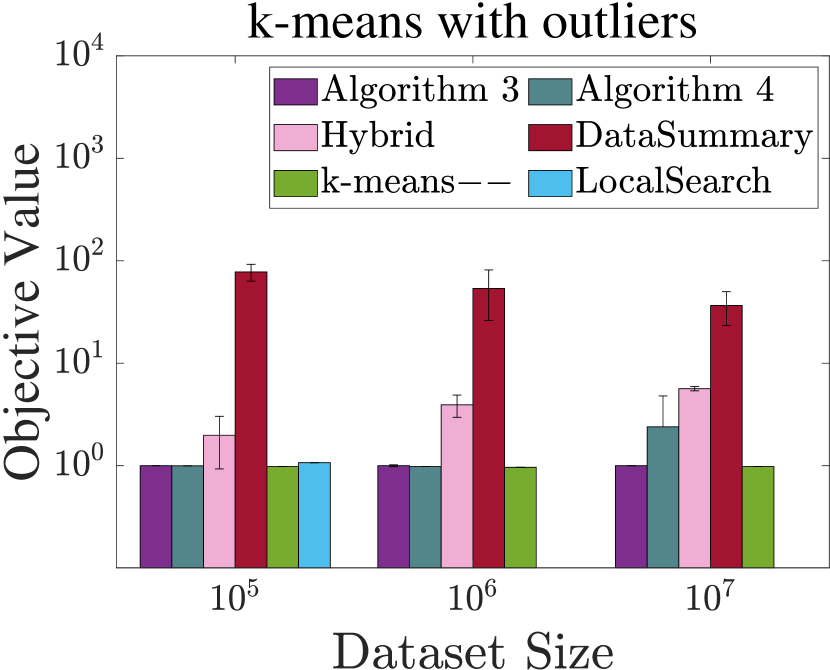
(b)

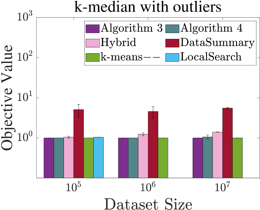
(c)

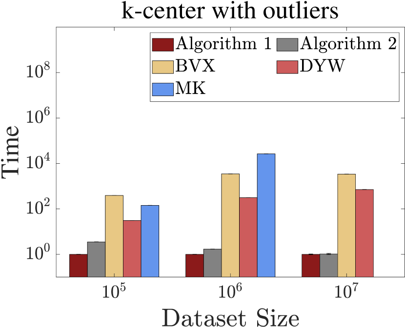
(d)

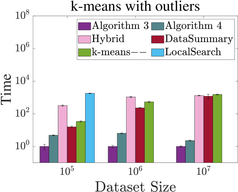
(e)

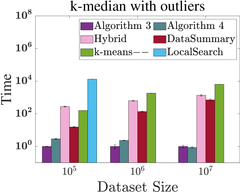
(f)

Figure 4: The normalized results (objective values and running times) on the synthetic datasets with varying $n$. We did not run Charikar, MK, Malkomes, and LocalSearch for large $n$ because their running times are too high. To illustrate the comparisons more clearly, we normalize all the results by dividing them over the results of Algorithm 1 with $\tau=2$ (resp., Algorithm 3 with $\tau=2$ ) for $k$-center (resp., $k$-means/median ) clustering with outliers.

We consider the scalability first. We enlarge the data size $n$ from $10^{5}$ to $10^{7}$, and illustrate the results in Figure 4. We fix the sampling size $|S|=10^{3}$. For Algorithm 1 and 3, we set $\tau=2$. We can see that our algorithms are several orders of magnitude faster than the baselines when $n$ is large. Actually, since our approach is just simple uniform sampling, the advantage over the non-uniform sampling approaches will be more significant when $n$ becomes large.

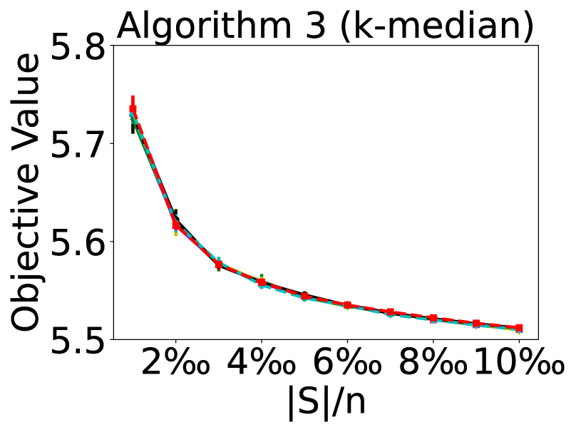
(e)

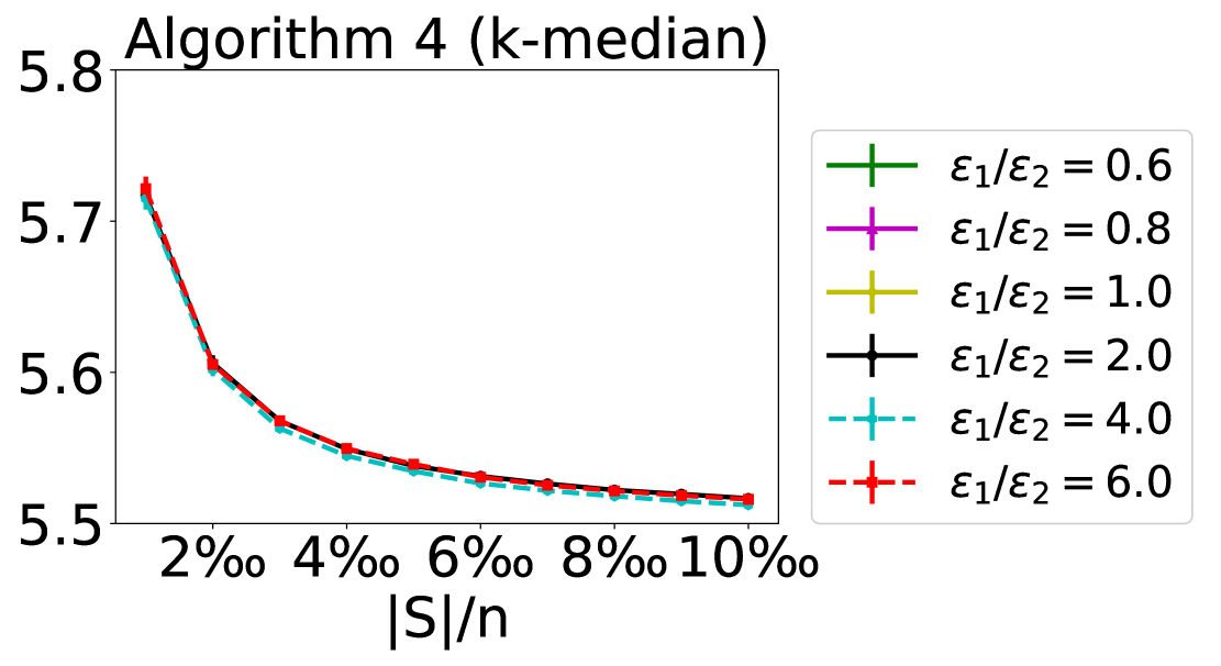
(f)

Figure 5: The performances with varying the sampling ratio $|S|/n$ (we run algorithm 2 and 4 for $\epsilon_{1}/\epsilon_{2}>1$).

We then study the influence of the sampling ratio $|S|/n$ to our algorithms. We vary $|S|/n$ from $1\times 10^{-3}$ to $10\times 10^{-3}$ and run our algorithms on the synthetic datasets. We show the results (averaged across $20$ trials) in Figure 5. We can see that the trends tend to be “flat” when the ratio $|S|/n>4\times 10^{-3}$.

4.3 Other Influence Factors

For completeness, we also consider several other influence factors. We fix the sampling ratio $|S|/n=5\times 10^{-3}$ as Section 2. As discussed before, the performances of Algorithm 2 and Algorithm 4 depend on the ratio $\epsilon_{1}/\epsilon_{2}$. An interesting question is that how about their stabilities in terms of $\epsilon_{1}/\epsilon_{2}$ (in particular, when $\epsilon_{1}/\epsilon_{2}\leq 1$). We repeat the experiments $20$ times on the synthetic datasets and compute the obtained average objective values and standard deviations. In Figure 6 (the two figures in the first line), we can see that their performances are actually quite stable when $\epsilon_{1}/\epsilon_{2}\geq 2$. This also agrees with our previous theoretical analysis, that is, larger $\epsilon_{1}/\epsilon_{2}$ is more friendly to uniform sampling.

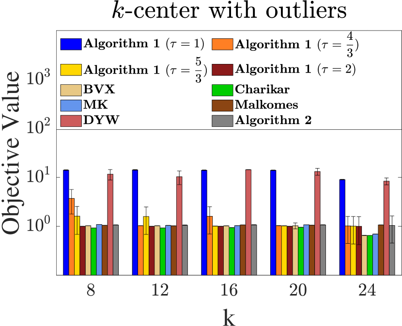
(a)

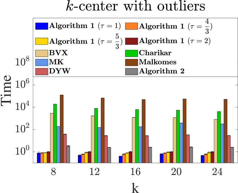
(b)

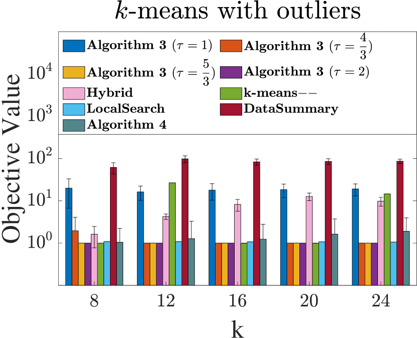
(c)

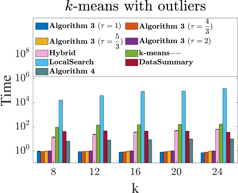
(d)

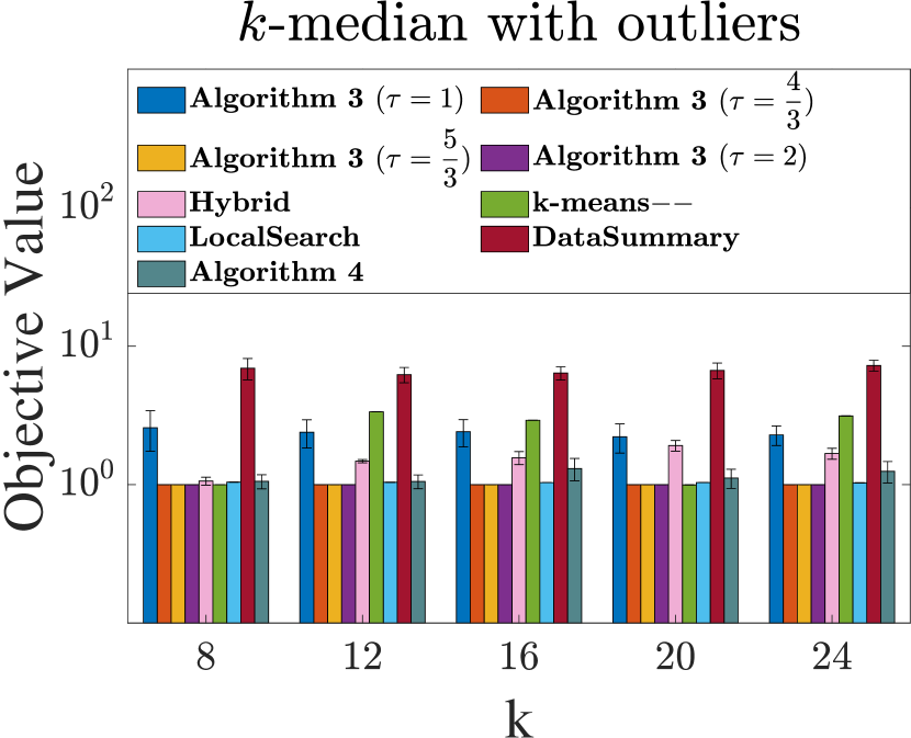
(e)

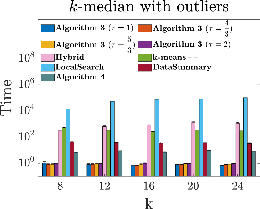
(f)

Figure 7: The normalized results (objective values and running times) on the synthetic datasets with varying $k$ (we set $z=2\%n$ and $\epsilon_{1}/\epsilon_{2}=2$). To illustrate the comparisons more clearly, we normalize all the results by dividing them over the results of Algorithm 1 with $\tau=2$ (resp., Algorithm 3 with $\tau=2$ ) for $k$-center (resp., $k$-means/median ) clustering with outliers.

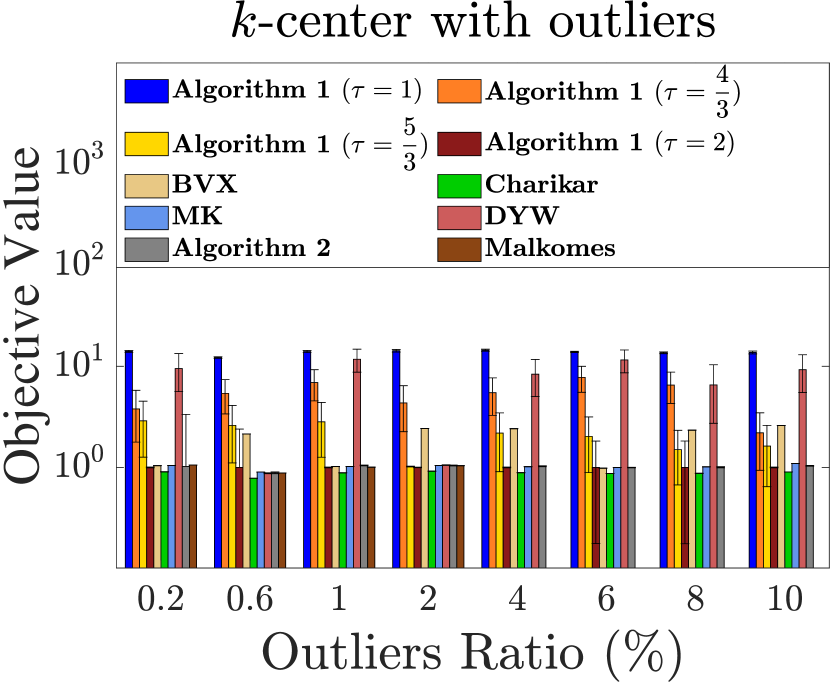
(a)

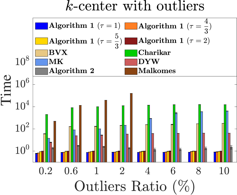
(b)

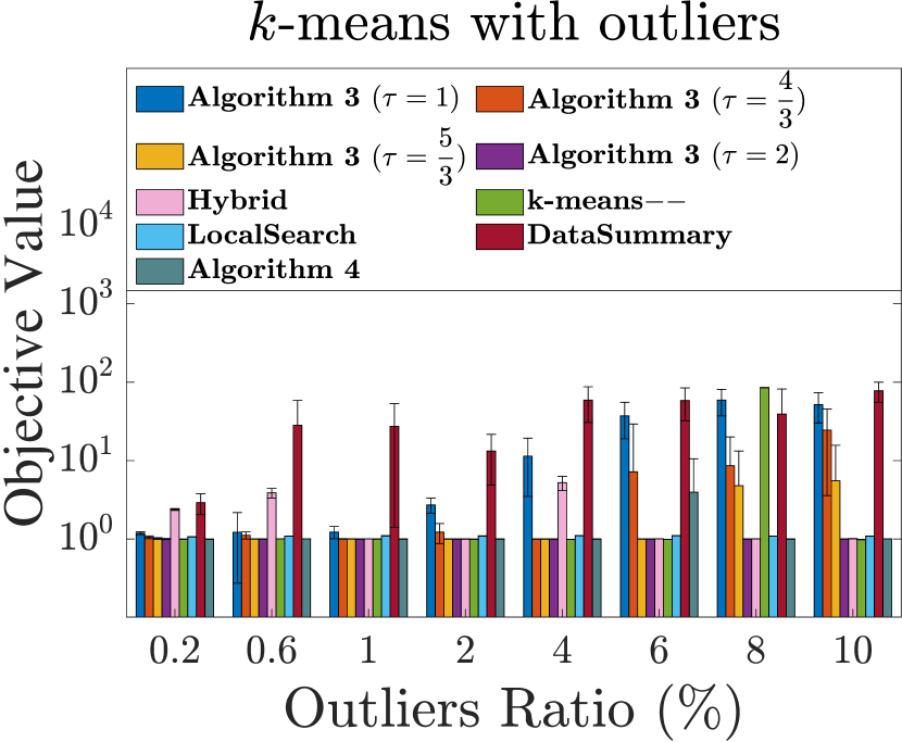
(c)

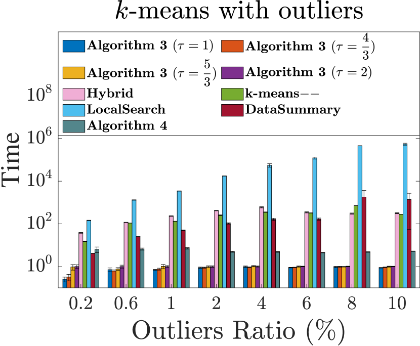
(d)

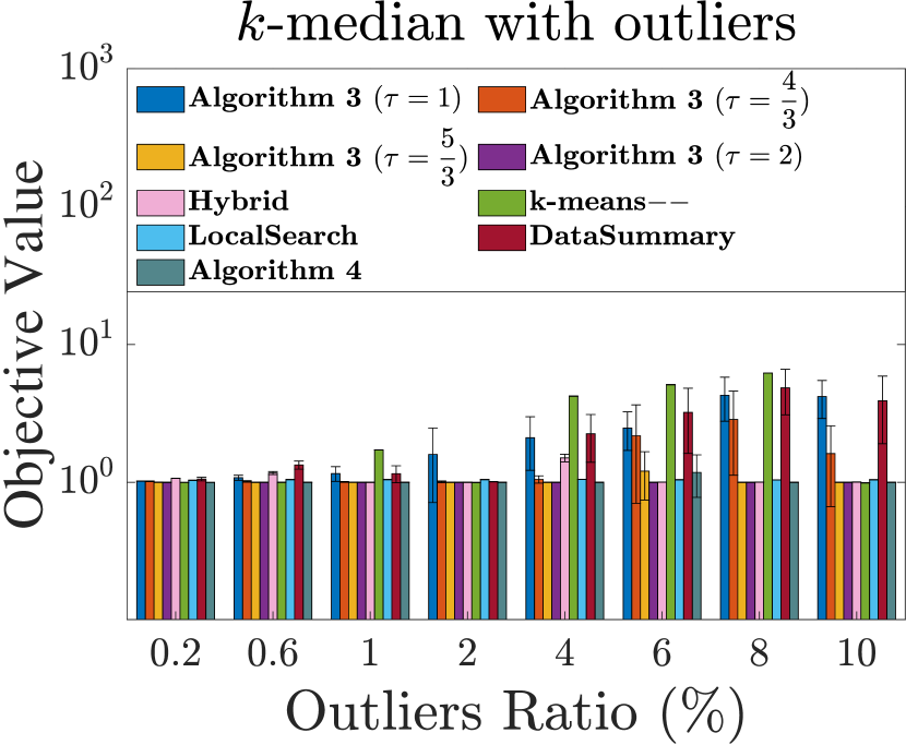
(e)

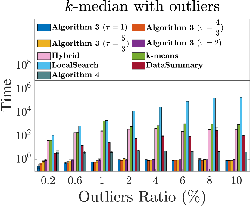
(f)

Figure 8: The normalized results (objective values and running times) on the synthetic datasets with varying $z/n$ (we set $k=4$ and $\epsilon_{1}/\epsilon_{2}=2$). We did not run Malkomes for $z/n\geq 4\%$, since it is very slow for large $z$. To illustrate the comparisons more clearly, we normalize all the results by dividing them over the results of Algorithm 1 with $\tau=2$ (resp., Algorithm 3 with $\tau=2$ ) for $k$-center (resp., $k$-means/median ) clustering with outliers.

In Figure 6 (the two figures in the second line), we study the influence of $\hat{z}$ on the performances (averaged across $20$ times). We vary $\hat{z}/\tilde{z}$ from $1.1$ to $2$, where $\tilde{z}=\frac{\epsilon_{2}}{k}|S|$ is the expected number of outliers contained in $S$. We also illustrate the experimental results on the synthetic datasets with varying $k$ from $8$ to $24$, and $z$ from $0.2\%n$ to $10\%n$, in Figure 7 and Figure 8 respectively. Overall, we observe that the influences from these parameters to the clustering qualities of our algorithms are relatively limited. And in general, our algorithms are considerably faster than the baseline algorithms.

5 Future Work

In this paper, we study the effectiveness of uniform sampling for center-based clustering with outliers problems. Following this work, an interesting question is that whether the significance measure (or some other realistic assumptions) can be applied to analyze uniform sampling for other robust optimization problems, such as PCA with outliers [50] and projective clustering with outliers [51].

Acknowledgements

The research of this work was supported in part by National Key R&D program of China through grant 2021YFA1000900, the NSFC throught Grant 62272432, and the Provincial NSF of Anhui through grant 2208085MF163.

Appendix A Extensions

A.1 For $k$-median clustering with outliers

The results of Theorem 3 and Theorem 4 can be easily extended to $k$-median clustering with outliers in Euclidean space by using almost the same idea, where the only difference is that we can directly use triangle inequality in the proofs (e.g., the inequality (14) is replaced by $||\tilde{q}-h_{\tilde{j}_{q}}||\leq||\tilde{q}-q||+||q-h_{j_{q}}||$). As a consequence, the coefficients $\alpha$ and $\beta$ are reduced to be $\big{(}1+(1+c)\frac{1+\delta}{1-\delta}\big{)}$ and $(1+c)\frac{1+\delta}{1-\delta}$ in Theorem 3, respectively. Similarly, $\alpha$ and $\beta$ are reduced to be $\big{(}1+(1+c)\frac{t}{t-1}\frac{1+\delta}{1-\delta}\big{)}$ and $(1+c)\frac{t}{t-1}\frac{1+\delta}{1-\delta}$ in Theorem 4.

A.2 For the general metric

To solve the metric $k$-median/means clustering with outliers problems for a given instance $(X,\mu)$, we should keep in mind that the cluster centers can only be selected from the vertices of $X$. However, the optimal cluster centers $O^{*}=\{o^{*}_{1},\cdots,o^{*}_{k}\}$ may not be contained in the sample $S$, and thus we need to modify our analysis slightly. We observe that the sample $S$ contains a set $O^{\prime}$ of vertices close to $O^{*}$ with certain probability. Specifically, for each $1\leq j\leq k$, there exists a vertex $o^{\prime}_{j}\in O^{\prime}$ such that $\mu(o^{\prime}_{j},o^{*}_{j})\leq O(1)\times\frac{1}{|C^{*}_{j}|}\sum_{p\in C^{*}_{j}}\mu(p,o^{*}_{j})$ (or $\big{(}\mu(o^{\prime}_{j},o^{*}_{j})\big{)}^{2}\leq O(1)\times\frac{1}{|C^{*}_{j}|}\sum_{p\in C^{*}_{j}}\big{(}\mu(p,o^{*}_{j})\big{)}^{2}$) with constant probability (this claim can be easily proved by using the Markov’s inequality). Consequently, we can use $O^{\prime}$ to replace $O^{*}$ in our analysis, and achieve the similar results as Theorem 3 and Theorem 4.

Table 1: Precision and Purity on real datasets ($k$-center with outliers)

Datasets	Shuttle		Kddcup		Covtype		Poking Hand
Measure	Prec	Purity	Prec	Purity	Prec	Purity	Prec	Purity
Algorithm 1 $\tau=1$	0.855	0.807	0.900	0.822	0.879	0.481	0.996	0.502
Algorithm 1 $\tau=\frac{4}{3}$	0.856	0.824	0.906	0.834	0.895	0.491	0.986	0.502
Algorithm 1 $\tau=\frac{5}{3}$	0.860	0.843	0.912	0.851	0.902	0.488	0.992	0.501
Algorithm 1 $\tau=2$	0.864	0.869	0.929	0.848	0.918	0.495	0.998	0.503
Algorithm 2	0.856	0.851	0.936	0.854	0.879	0.493	0.936	0.503
BVX	0.908	0.786	0.945	0.574	0.879	0.487	0.998	0.501
MK	0.886	0.828	0.914	0.832	0.879	0.488	0.982	0.502
Malkomes	0.862	0.790	0.918	0.841	0.902	0.501	0.992	0.504
DYW	0.853	0.813	0.912	0.850	0.899	0.502	0.981	0.510

Table 2: Precision and Purity on real datasets ($k$-means with outliers)

Datasets	Shuttle		Kddcup		Covtype		Poking Hand
Measure	Prec	Purity	Prec	Purity	Prec	Purity	Prec	Purity
Algorithm 3 $\tau=1$	0.857	0.883	0.948	0.988	0.879	0.507	0.982	0.501
Algorithm 3 $\tau=\frac{4}{3}$	0.852	0.922	0.962	0.986	0.889	0.522	0.996	0.502
Algorithm 3 $\tau=\frac{5}{3}$	0.855	0.914	0.955	0.989	0.913	0.527	0.999	0.505
Algorithm 3 $\tau=2$	0.861	0.944	0.972	0.991	0.906	0.515	0.999	0.506
Algorithm 4	0.856	0.867	0.927	0.982	0.906	0.523	0.999	0.510
Hybrid	0.858	0.903	0.899	0.992	0.884	0.534	0.999	0.501
$k$-means$--$	0.872	0.842	0.915	0.985	0.879	0.537	0.999	0.502
LocalSearch	0.857	0.915	0.929	0.989	0.876	0.541	0.998	0.501
DataSummary	0.857	0.920	0.865	0.994	0.880	0.512	0.990	0.501

(a)

(b)

(c)

(d)

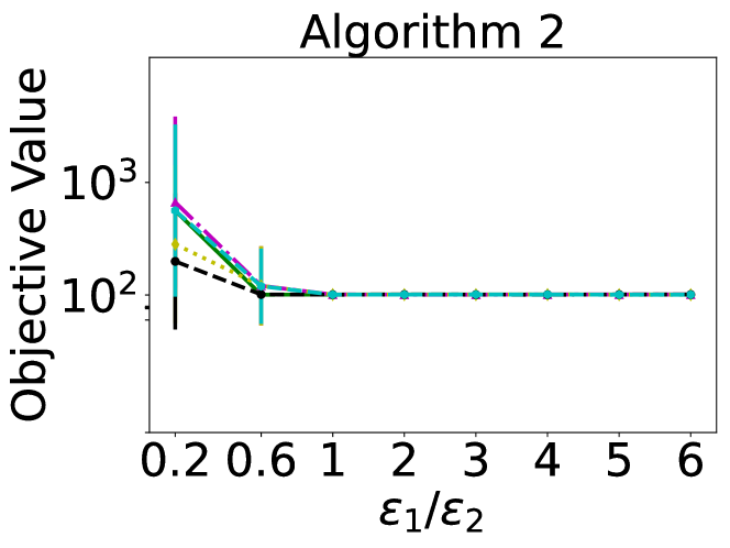
(a) Varying $\epsilon_{1}/\epsilon_{2}$ for Algorithm 2

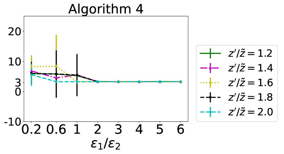
(b) Varying $\epsilon_{1}/\epsilon_{2}$ for Algorithm 4

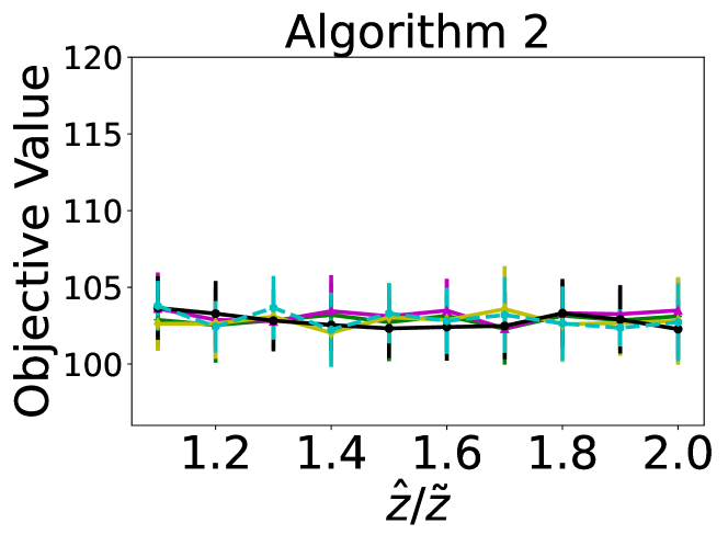
(c) Varying $\hat{z}/\tilde{z}$ for Algorithm 2

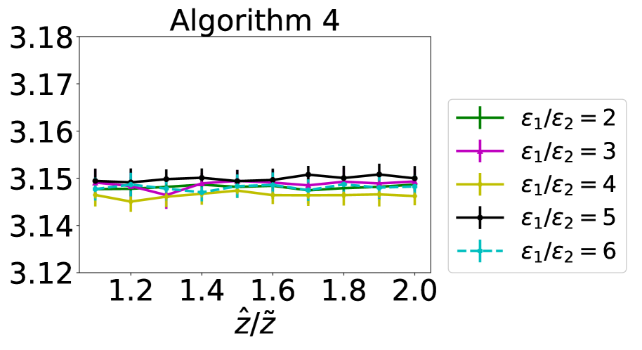
(d) Varying $\hat{z}/\tilde{z}$ for Algorithm 4

Figure 6: The average objective values and standard deviations with varying $\epsilon_{1}/\epsilon_{2}$ and $\hat{z}/\tilde{z}$. $\tilde{z}=\frac{\epsilon_{2}}{k}|S|$ is the expected number of outliers contained in $S$.

References

- Jain [2010] Anil K Jain. Data clustering: 50 years beyond k-means. Pattern recognition letters, 31(8):651–666, 2010.
- Awasthi and Balcan [2014] Pranjal Awasthi and Maria-Florina Balcan. Center based clustering: A foundational perspective. 2014.
- Georgogiannis [2016] Alexandros Georgogiannis. Robust k-means: a theoretical revisit. Advances in Neural Information Processing Systems, 29, 2016.
- Chandola et al. [2009] Varun Chandola, Arindam Banerjee, and Vipin Kumar. Anomaly detection: A survey. ACM Computing Surveys (CSUR), 41(3):15, 2009.
- Ester et al. [1996] Martin Ester, Hans-Peter Kriegel, Jörg Sander, and Xiaowei Xu. A density-based algorithm for discovering clusters in large spatial databases with noise. In Proceedings of the ACM SIGKDD International Conference on Knowledge Discovery and Data Mining (KDD), pages 226–231, 1996.
- Bhattacharjee and Mitra [2021] Panthadeep Bhattacharjee and Pinaki Mitra. A survey of density based clustering algorithms. Frontiers of Computer Science, 15:1–27, 2021.
- Sener and Savarese [2018] Ozan Sener and Silvio Savarese. Active learning for convolutional neural networks: A core-set approach. In 6th International Conference on Learning Representations, ICLR 2018, Vancouver, BC, Canada, April 30 - May 3, 2018, Conference Track Proceedings. OpenReview.net, 2018.
- Coleman et al. [2020] Cody Coleman, Christopher Yeh, Stephen Mussmann, Baharan Mirzasoleiman, Peter Bailis, Percy Liang, Jure Leskovec, and Matei Zaharia. Selection via proxy: Efficient data selection for deep learning. In International Conference on Learning Representations, 2020.
- Charikar et al. [2001] Moses Charikar, Samir Khuller, David M Mount, and Giri Narasimhan. Algorithms for facility location problems with outliers. In Proceedings of the twelfth annual ACM-SIAM symposium on Discrete algorithms, pages 642–651. Society for Industrial and Applied Mathematics, 2001.
- Gupta et al. [2017] Shalmoli Gupta, Ravi Kumar, Kefu Lu, Benjamin Moseley, and Sergei Vassilvitskii. Local search methods for k-means with outliers. Proceedings of the VLDB Endowment, 10(7):757–768, 2017.
- Im et al. [2020] Sungjin Im, Mahshid Montazer Qaem, Benjamin Moseley, Xiaorui Sun, and Rudy Zhou. Fast noise removal for k-means clustering. In Proceedings of the Twenty Third International Conference on Artificial Intelligence and Statistics, Proceedings of Machine Learning Research. PMLR, 2020.
- Bhaskara et al. [2019] Aditya Bhaskara, Sharvaree Vadgama, and Hong Xu. Greedy sampling for approximate clustering in the presence of outliers. In Advances in Neural Information Processing Systems, volume 32. Curran Associates, Inc., 2019.
- Deshpande et al. [2020] Amit Deshpande, Praneeth Kacham, and Rameshwar Pratap. Robust k-means++. In Proceedings of the 36th Conference on Uncertainty in Artificial Intelligence (UAI), volume 124 of Proceedings of Machine Learning Research, pages 799–808. AUAI Press, 2020.
- Chen et al. [2018] Jiecao Chen, Erfan Sadeqi Azer, and Qin Zhang. A practical algorithm for distributed clustering and outlier detection. In Advances in Neural Information Processing Systems, pages 2253–2262, 2018.
- Sanders [2014] Peter Sanders. Algorithm engineering for big data. In Erhard Plödereder, Lars Grunske, Eric Schneider, and Dominik Ull, editors, 44. Jahrestagung der Gesellschaft für Informatik, Big Data - Komplexität meistern, INFORMATIK 2014, Stuttgart, Germany, September 22-26, 2014, volume P-232 of LNI, page 57. GI, 2014.
- Huang et al. [2018] Lingxiao Huang, Shaofeng Jiang, Jian Li, and Xuan Wu. Epsilon-coresets for clustering (with outliers) in doubling metrics. In 2018 IEEE 59th Annual Symposium on Foundations of Computer Science (FOCS), pages 814–825. IEEE, 2018.
- Meyerson et al. [2004] Adam Meyerson, Liadan O’callaghan, and Serge Plotkin. A k-median algorithm with running time independent of data size. Machine Learning, 56(1-3):61–87, 2004.
- Charikar et al. [2003] Moses Charikar, Liadan O’Callaghan, and Rina Panigrahy. Better streaming algorithms for clustering problems. In Proceedings of the thirty-fifth annual ACM symposium on Theory of computing, pages 30–39. ACM, 2003.
- Ding et al. [2019] Hu Ding, Haikuo Yu, and Zixiu Wang. Greedy strategy works for k-center clustering with outliers and coreset construction. In 27th Annual European Symposium on Algorithms, ESA 2019, September 9-11, 2019, Munich/Garching, Germany, pages 40:1–40:16, 2019.
- Gupta [2018] Shalmoli Gupta. Approximation algorithms for clustering and facility location problems. PhD thesis, University of Illinois at Urbana-Champaign, 2018.
- McCutchen and Khuller [2008] Richard Matthew McCutchen and Samir Khuller. Streaming algorithms for k-center clustering with outliers and with anonymity. In Approximation, Randomization and Combinatorial Optimization. Algorithms and Techniques, pages 165–178. Springer, 2008.
- Chakrabarty et al. [2016] Deeparnab Chakrabarty, Prachi Goyal, and Ravishankar Krishnaswamy. The non-uniform k-center problem. In 43rd International Colloquium on Automata, Languages, and Programming, ICALP 2016, July 11-15, 2016, Rome, Italy, pages 67:1–67:15, 2016.
- Bădoiu et al. [2002] Mihai Bădoiu, Sariel Har-Peled, and Piotr Indyk. Approximate clustering via core-sets. In Proceedings of the ACM Symposium on Theory of Computing (STOC), pages 250–257, 2002.
- Gonzalez [1985] Teofilo F Gonzalez. Clustering to minimize the maximum intercluster distance. Theoretical Computer Science, 38:293–306, 1985.
- Ceccarello et al. [2019] Matteo Ceccarello, Andrea Pietracaprina, and Geppino Pucci. Solving k-center clustering (with outliers) in mapreduce and streaming, almost as accurately as sequentially. PVLDB, 12(7):766–778, 2019.
- Cuesta-Albertos et al. [1997] J. A. Cuesta-Albertos, A. Gordaliza, and C. Matran. Trimmed k-means: An attempt to robustify quantizers. The Annals of Statistics, 25(2):553–576, 1997. ISSN 00905364.
- Chen [2008] Ke Chen. A constant factor approximation algorithm for k-median clustering with outliers. In Proceedings of the nineteenth annual ACM-SIAM symposium on Discrete algorithms, pages 826–835. Society for Industrial and Applied Mathematics, 2008.
- Krishnaswamy et al. [2018] Ravishankar Krishnaswamy, Shi Li, and Sai Sandeep. Constant approximation for k-median and k-means with outliers via iterative rounding. In Proceedings of the 50th Annual ACM SIGACT Symposium on Theory of Computing, pages 646–659. ACM, 2018.
- Friggstad et al. [2018] Zachary Friggstad, Kamyar Khodamoradi, Mohsen Rezapour, and Mohammad R Salavatipour. Approximation schemes for clustering with outliers. In Proceedings of the Twenty-Ninth Annual ACM-SIAM Symposium on Discrete Algorithms, pages 398–414. SIAM, 2018.
- Chawla and Gionis [2013] Sanjay Chawla and Aristides Gionis. k-means–: A unified approach to clustering and outlier detection. In Proceedings of the 2013 SIAM International Conference on Data Mining, pages 189–197. SIAM, 2013.
- Ott et al. [2014] Lionel Ott, Linsey Pang, Fabio T Ramos, and Sanjay Chawla. On integrated clustering and outlier detection. In Advances in neural information processing systems, pages 1359–1367, 2014.
- Liu et al. [2019] Hongfu Liu, Jun Li, Yue Wu, and Yun Fu. Clustering with outlier removal. IEEE transactions on knowledge and data engineering, 33(6):2369–2379, 2019.
- Paul et al. [2021] Debolina Paul, Saptarshi Chakraborty, Swagatam Das, and Jason Xu. Uniform concentration bounds toward a unified framework for robust clustering. Advances in Neural Information Processing Systems, 34, 2021.
- Arthur and Vassilvitskii [2007] David Arthur and Sergei Vassilvitskii. k-means++: The advantages of careful seeding. In Proceedings of the eighteenth annual ACM-SIAM symposium on Discrete algorithms, pages 1027–1035. Society for Industrial and Applied Mathematics, 2007.
- Mettu and Plaxton [2004] Ramgopal R Mettu and C Greg Plaxton. Optimal time bounds for approximate clustering. Machine Learning, 56(1-3):35–60, 2004.
- Ding and Wang [2020] Hu Ding and Zixiu Wang. Layered sampling for robust optimization problems. In Proceedings of the 37th International Conference on Machine Learning, ICML, volume 119, pages 2556–2566, 2020.
- Huang et al. [2023] Lingxiao Huang, Shaofeng H-C Jiang, Jianing Lou, and Xuan Wu. Near-optimal coresets for robust clustering. International Conference on Learning Representations, ICLR, 2023.
- Braverman et al. [2022] Vladimir Braverman, Vincent Cohen-Addad, H-C Shaofeng Jiang, Robert Krauthgamer, Chris Schwiegelshohn, Mads Bech Toftrup, and Xuan Wu. The power of uniform sampling for coresets. In 2022 IEEE 63rd Annual Symposium on Foundations of Computer Science (FOCS), pages 462–473. IEEE, 2022.
- Indyk [1999] Piotr Indyk. Sublinear time algorithms for metric space problems. In Proceedings of the Thirty-First Annual ACM Symposium on Theory of Computing, May 1-4, 1999, Atlanta, Georgia, USA, pages 428–434, 1999.
- Mishra et al. [2001] Nina Mishra, Dan Oblinger, and Leonard Pitt. Sublinear time approximate clustering. In Proceedings of the twelfth annual ACM-SIAM symposium on Discrete algorithms, pages 439–447. Society for Industrial and Applied Mathematics, 2001.
- Czumaj and Sohler [2004] Artur Czumaj and Christian Sohler. Sublinear-time approximation for clustering via random sampling. In International Colloquium on Automata, Languages, and Programming, pages 396–407. Springer, 2004.
- Goldreich et al. [1998] Oded Goldreich, Shafi Goldwasser, and Dana Ron. Property testing and its connection to learning and approximation. J. ACM, 45(4):653–750, 1998.
- Ding and Xu [2014] Hu Ding and Jinhui Xu. Sub-linear time hybrid approximations for least trimmed squares estimator and related problems. In Proceedings of the International Symposium on Computational geometry (SoCG), page 110, 2014.
- Alon and Spencer [2004] Noga Alon and Joel H Spencer. The probabilistic method. John Wiley & Sons, 2004.
- Kanungo et al. [2004] Tapas Kanungo, David M Mount, Nathan S Netanyahu, Christine D Piatko, Ruth Silverman, and Angela Y Wu. A local search approximation algorithm for k-means clustering. Computational Geometry, 28(2-3):89–112, 2004.
- Malkomes et al. [2015] Gustavo Malkomes, Matt J Kusner, Wenlin Chen, Kilian Q Weinberger, and Benjamin Moseley. Fast distributed k-center clustering with outliers on massive data. In Advances in Neural Information Processing Systems, pages 1063–1071, 2015.
- Bachem et al. [2016] Olivier Bachem, Mario Lucic, S. Hamed Hassani, and Andreas Krause. Fast and provably good seedings for k-means. In Proceedings of the 30th International Conference on Neural Information Processing Systems, NIPS’16, page 55–63, Red Hook, NY, USA, 2016. Curran Associates Inc. ISBN 9781510838819.
- Dua and Graff [2017] Dheeru Dua and Casey Graff. UCI machine learning repository, 2017. URL http://archive.ics.uci.edu/ml.
- Manning et al. [2008] Christopher D. Manning, Prabhakar Raghavan, and Hinrich Schütze. Introduction to information retrieval. Cambridge University Press, 2008. ISBN 978-0-521-86571-5. 10.1017/CBO9780511809071.
- Candès et al. [2011] Emmanuel J. Candès, Xiaodong Li, Yi Ma, and John Wright. Robust principal component analysis? J. ACM, 58(3):11:1–11:37, 2011.
- Feldman and Langberg [2011] Dan Feldman and Michael Langberg. A unified framework for approximating and clustering data. In Proceedings of the forty-third annual ACM symposium on Theory of computing, pages 569–578. ACM, 2011.