Block-Activated Algorithms for Multicomponent Fully Nonsmooth Minimization

Abstract

Under consideration are multicomponent minimization problems involving a separable nonsmooth convex function penalizing the components individually, and nonsmooth convex coupling terms penalizing linear mixtures of the components. We investigate block-activated proximal algorithms for solving such problems, i.e., algorithms which, at each iteration, need to use only a block of the underlying functions, as opposed to all of them as in standard methods. For smooth coupling functions, several block-activated algorithms exist and they are well understood. By contrast, in the fully nonsmooth case, few block-activated methods are available and little effort has been devoted to assessing them. Our goal is to shed more light on the implementation, the features, and the behavior of these algorithms, compare their merits, and provide machine learning and image recovery experiments illustrating their performance.

1 Introduction

The goal of many signal processing and machine learning tasks is to exploit the observed data and the prior knowledge to produce a solution that represents information of interest. In this process of extracting information from data, structured convex optimization has established itself as an effective modeling and algorithmic framework; see, for instance, [3, 5, 8, 14, 19]. In state-of-the-art applications, the sought solution is often a tuple of vectors which reside in different spaces [1, 2, 4, 6, 12, 16, 13, 17, 20]. The following multicomponent minimization formulation captures such problems. It consists of a separable term penalizing the components individually, and of coupling terms penalizing linear mixtures of the components.

Problem 1

Let $({\mathcal{H}}_{i})_{1\leqslant i\leqslant m}$ and $({\mathcal{G}}_{k})_{1\leqslant k\leqslant p}$ be Euclidean spaces. For every $i\in\{1,\ldots,m\}$ and every $k\in\{1,\ldots,p\}$, let $f_{i}\colon{\mathcal{H}}_{i}\to\left]{-}\infty,{+}\infty\right]$ and $g_{k}\colon{\mathcal{G}}_{k}\to\left]{-}\infty,{+}\infty\right]$ be proper lower semicontinuous convex functions, and let $L_{k,i}\colon{\mathcal{H}}_{i}\to{\mathcal{G}}_{k}$ be a linear operator. The objective is to

$$\underset{x_{1}\in{\mathcal{H}}_{1},\ldots,x_{m}\in{\mathcal{H}}_{m}}{\operatorname{minimize}}\;\>\underbrace{\sum_{i=1}^{m}f_{i}(x_{i})}_{\text{separable term}}+\sum_{k=1}^{p}\underbrace{g_{k}\Bigg{(}\sum_{i=1}^{m}L_{k,i}x_{i}\Bigg{)}}_{\text{$k$th coupling term}}.$$ (1)

To solve Problem 1 reliably without adding restrictions (for instance, smoothness or strong convexity of some functions involved in the model), we focus on flexible proximal algorithms that have the following features:

1. Nondifferentiability: None of the functions $f_{1},\ldots,$ $f_{m},g_{1},\ldots,g_{p}$ needs to be differentiable.

2. Splitting: The functions $f_{1},\ldots,f_{m},g_{1},\ldots,g_{p}$ and the linear operators are activated separately.

3. Block activation: Only a block of the functions $f_{1},\ldots,$ $f_{m},g_{1},\ldots,g_{p}$ is activated at each iteration. This is in contrast with most splitting methods which require full activation, i.e., that all the functions be used at every iteration.

4. Operator norms: Bounds on the norms of the linear operators involved in Problem 1 are not assumed since they can be hard to compute.

5. Convergence guarantee: The algorithm produces a sequence which converges (possibly almost surely) to a solution to Problem 1.

In view of features ➀ ‣ 1 and ➁ ‣ 1, the algorithms of interest should activate the functions $f_{1},\ldots,f_{m},g_{1},\ldots,g_{p}$ via their proximity operators (even if some functions happened to be smooth, proximal activation is often preferable [6, 10]). The motivation for ➁ ‣ 1 is that proximity operators of composite functions are typically not known explicitly. Feature ➂ ‣ 1 is geared towards current large-scale problems. In such scenarios, memory and computing power limitations make the execution of standard proximal splitting algorithms, which require activating all the functions at each iteration, inefficient or simply impossible. We must therefore turn our attention to algorithms which employ only blocks of functions $(f_{i})_{i\in I_{n}}$ and $(g_{k})_{k\in K_{n}}$ at iteration $n$. If the functions $(g_{k})_{1\leqslant k\leqslant p}$ were all smooth, one could use block-activated versions of the forward-backward algorithm proposed in [15, 25] and the references therein; in particular, when $m=1$, methods such as those of [11, 18, 23, 26] would be pertinent. As noted in [15, Remark 5.10(iv)], another candidate of interest could be the randomly block-activated algorithm of [15, Section 5.2], which leads to block-activated versions of several primal-dual methods (see [24] for detailed developments and [7] for an inertial version when $m=1$). However, this approach violates ➃ ‣ 1 as it imposes bounds on the proximal scaling parameters which depend on the norms of the linear operators. Finally, ➄ ‣ 1 rules out methods that guarantee merely minimizing sequences or ergodic convergence.

To the best of our knowledge, there are two primary methods that fulfill ➀ ‣ 1–➄ ‣ 1:

• Algorithm A: The stochastic primal-dual Douglas–Rachford algorithm of [15].

• Algorithm B: The deterministic primal-dual projective splitting algorithm of [9].

In the case of smooth coupling functions $(g_{k})_{1\leqslant k\leqslant p}$, in (1), extensive numerical experience has been accumulated to understand the behavior of block-activated methods, especially in the case of stochastic gradient methods. By contrast, to date, very few numerical experiments with the recent, fully nonsmooth Algorithms A and B have been conducted and no comparison of their merits and performance has been undertaken. Thus far, Algorithm A has been employed only in the context of machine learning (see also the variant of A in [6] for partially smooth problems). On the other hand, Algorithm B has been used in image recovery in [10], but only in full activation mode, and in feature selection in [22], but with $m=1$.

Contributions and novelty: This paper investigates for the first time the use of block-activated methods in fully nonsmooth multivariate minimization problems. It sheds more light on the implementation, the features, and the behavior of Algorithms A and B, compares their merits, and provides experiments illustrating their performance.

Outline: Algorithms A and B are presented in Section 2. In Section 3, we analyze and compare their features, implementation, and asymptotic properties. This investigation is complemented in Section 4 by numerical experiments in the context of machine learning and image recovery.

2 Block-Activated Algorithms for Problem 1

The subdifferential, the conjugate, and the proximity operator of a proper lower semicontinuous convex function $f\colon{\mathcal{H}}\to\left]{-}\infty,{+}\infty\right]$ are denoted by $\partial f$, $f^{*}$, and $\mathrm{prox}_{f}$, respectively. Let us consider the setting of Problem 1 and let us set $\boldsymbol{\mathcal{H}}={\mathcal{H}}_{1}\times\cdots\times{\mathcal{H}}_{m}$ and $\boldsymbol{\mathcal{G}}={\mathcal{G}}_{1}\times\cdots\times{\mathcal{G}}_{p}$. A generic element in $\boldsymbol{\mathcal{H}}$ is denoted by $\boldsymbol{x}=(x_{i})_{1\leqslant i\leqslant m}$ and a generic element in $\boldsymbol{\mathcal{G}}$ by $\boldsymbol{y}=(y_{k})_{1\leqslant k\leqslant p}$.

As discussed in Section 1, two primary algorithms fulfill requirements ➀ ‣ 1–➄ ‣ 1. Both operate in the product space $\boldsymbol{\mathcal{H}}\times\boldsymbol{\mathcal{G}}$. The first one employs random activation of the blocks. To present it, let us introduce

$$\begin{cases}\boldsymbol{L}\colon\boldsymbol{\mathcal{H}}\to\boldsymbol{\mathcal{G}}\colon\boldsymbol{x}\mapsto\bigg{(}\displaystyle\sum_{i=1}^{m}{L}_{1,i}x_{i},\ldots,\displaystyle\sum_{i=1}^{m}{L}_{p,i}x_{i}\bigg{)}\\ \boldsymbol{V}=\big{\{}{(\boldsymbol{x},\boldsymbol{y})\in\boldsymbol{\mathcal{H}}\times\boldsymbol{\mathcal{G}}}~{}|~{}{\boldsymbol{y}=\boldsymbol{L}\boldsymbol{x}}\big{\}}\\ \boldsymbol{F}\colon\boldsymbol{\mathcal{H}}\times\boldsymbol{\mathcal{G}}\to\left]{-}\infty,{+}\infty\right]\\ ~{}~{}~{}~{}\hskip 5.406pt(\boldsymbol{x},\boldsymbol{y})\mapsto\sum_{i=1}^{m}f_{i}(x_{i})+\sum_{k=1}^{p}g_{k}(y_{k}).\end{cases}$$ (2)

Then (1) is equivalent to

$$\underset{(\boldsymbol{x},\boldsymbol{y})\in\boldsymbol{V}}{\operatorname{minimize}}\;\>\boldsymbol{F}(\boldsymbol{x},\boldsymbol{y}).$$ (3)

The idea is then to apply the Douglas–Rachford algorithm in block form to this problem [15]. To this end, we need $\mathrm{prox}_{\boldsymbol{F}}$ and $\mathrm{prox}_{\iota_{\boldsymbol{V}}}=\mathrm{proj}_{\boldsymbol{V}}$. Note that $\mathrm{prox}_{\boldsymbol{F}}\colon(\boldsymbol{x},\boldsymbol{y})\mapsto((\mathrm{prox}_{f_{i}}x_{i})_{1\leqslant i\leqslant m},(\mathrm{prox}_{g_{k}}y_{k})_{1\leqslant k\leqslant p})$. Now let $\boldsymbol{x}\in\boldsymbol{\mathcal{H}}$ and $\boldsymbol{y}\in\boldsymbol{\mathcal{G}}$, and set $\boldsymbol{t}=(\mathbf{Id}+\boldsymbol{L}^{*}\boldsymbol{L})^{-1}(\boldsymbol{x}+\boldsymbol{L}^{*}\boldsymbol{y})$ and $\boldsymbol{s}=(\mathbf{Id}+\boldsymbol{L}\boldsymbol{L}^{*})^{-1}(\boldsymbol{L}\boldsymbol{x}-\boldsymbol{y})$. Then

$$\mathrm{proj}_{\boldsymbol{V}}(\boldsymbol{x},\boldsymbol{y})=(\boldsymbol{t},\boldsymbol{L}\boldsymbol{t})=(\boldsymbol{x}-\boldsymbol{L}^{*}\boldsymbol{s},\boldsymbol{y}+\boldsymbol{s}),$$ (4)

and we write it coordinate-wise as

$$\mathrm{proj}_{\boldsymbol{V}}(\boldsymbol{x},\boldsymbol{y})=\big{(}Q_{1}(\boldsymbol{x},\boldsymbol{y}),\ldots,Q_{m+p}(\boldsymbol{x},\boldsymbol{y})\big{)}.$$ (5)

Thus, given $\gamma\in\left]0,{+}\infty\right[$, $\boldsymbol{z}_{0}\in\boldsymbol{\mathcal{H}}$, and $\boldsymbol{y}_{0}\in\boldsymbol{\mathcal{G}}$, the standard Douglas–Rachford algorithm for (3) is

$$\begin{array}[]{l}\text{for}\;n=0,1,\ldots\\ \left\lfloor\begin{array}[]{l}\lambda_{n}\in\left]0,2\right[\\ \text{for every}\;i\in\{1,\ldots,m\}\\ \left\lfloor\begin{array}[]{l}x_{i,n+1}=Q_{i}(\boldsymbol{z}_{n},\boldsymbol{y}_{n})\\ z_{i,n+1}=z_{i,n}+\lambda_{n}\big{(}\mathrm{prox}_{\gamma f_{i}}(2x_{i,n+1}-z_{i,n})-x_{i,n+1}\big{)}\end{array}\right.\\ \text{for every}\;k\in\{1,\ldots,p\}\\ \left\lfloor\begin{array}[]{l}w_{k,n+1}=Q_{m+k}(\boldsymbol{z}_{n},\boldsymbol{y}_{n})\\ y_{k,n+1}=y_{k,n}+\lambda_{n}\big{(}\mathrm{prox}_{\gamma g_{k}}(2w_{k,n+1}-y_{k,n})-w_{k,n+1}\big{)}.\end{array}\right.\\[17.07164pt] \end{array}\right.\end{array}$$ (6)

The block-activated version of this algorithm is as follows.

Algorithm A ([15])

Let $\gamma\in\left]0,{+}\infty\right[$, let $\boldsymbol{x}_{0}$ and $\boldsymbol{z}_{0}$ be $\boldsymbol{\mathcal{H}}$-valued random variables (r.v.), let $\boldsymbol{y}_{0}$ and $\boldsymbol{w}_{0}$ be $\boldsymbol{\mathcal{G}}$-valued r.v. Iterate

$$\hskip-8.53581pt\begin{array}[]{l}\text{for}\;j=1,\ldots,m+p\\ \left\lfloor\text{compute}\;Q_{j}\;\text{as in \eqref{e:o7}--\eqref{e:o8}}\right.\\ \text{for}\;n=0,1,\ldots\\ \left\lfloor\begin{array}[]{l}\lambda_{n}\in\left]0,2\right[\\ \text{select randomly}\;\varnothing\neq I_{n}\subset\{1,\ldots,m\}\;\text{and}\;\varnothing\neq K_{n}\subset\{1,\ldots,p\}\\ \text{for every}\;i\in I_{n}\\ \left\lfloor\begin{array}[]{l}x_{i,n+1}=Q_{i}(\boldsymbol{z}_{n},\boldsymbol{y}_{n})\\ z_{i,n+1}=z_{i,n}+\lambda_{n}\big{(}\mathrm{prox}_{\gamma f_{i}}(2x_{i,n+1}-z_{i,n})-x_{i,n+1}\big{)}\end{array}\right.\\ \text{for every}\;i\in\{1,\ldots,m\}\smallsetminus I_{n}\\ \left\lfloor\begin{array}[]{l}(x_{i,n+1},z_{i,n+1})=(x_{i,n},z_{i,n})\end{array}\right.\\ \text{for every}\;k\in K_{n}\\ \left\lfloor\begin{array}[]{l}w_{k,n+1}=Q_{m+k}(\boldsymbol{z}_{n},\boldsymbol{y}_{n})\\ y_{k,n+1}=y_{k,n}+\lambda_{n}\big{(}\mathrm{prox}_{\gamma g_{k}}(2w_{k,n+1}-y_{k,n})-w_{k,n+1}\big{)}\end{array}\right.\\ \text{for every}\;k\in\{1,\ldots,p\}\smallsetminus K_{n}\\ \left\lfloor\begin{array}[]{l}(w_{k,n+1},y_{k,n+1})=(w_{k,n},y_{k,n}).\end{array}\right.\\[5.69054pt] \end{array}\right.\end{array}$$

The second algorithm operates by projecting onto hyperplanes which separate the current iterate from the set $\boldsymbol{\mathsf{Z}}$ of Kuhn–Tucker points of Problem 1, i.e., the points $\widetilde{\boldsymbol{x}}\in\boldsymbol{\mathcal{H}}$ and $\widetilde{\boldsymbol{v}}^{*}\in\boldsymbol{\mathcal{G}}$ such that

$$\begin{cases}(\forall i\in\{1,\ldots,m\})\quad{-}\sum_{k=1}^{p}L_{k,i}^{*}\widetilde{v}_{k}^{*}\in\partial f_{i}(\widetilde{x}_{i})\\ (\forall k\in\{1,\ldots,p\})\quad\sum_{i=1}^{m}L_{k,i}\widetilde{x}_{i}\in\partial g_{k}^{*}(\widetilde{v}_{k}^{*}).\end{cases}$$ (7)

This process is explained in Fig. 1.

Algorithm B ([9])

Set $I_{0}=\{1,\ldots,m\}$ and $K_{0}=\{1,\ldots,p\}$. For every $i\in I_{0}$ and every $k\in K_{0}$, let $\{\gamma_{i},\mu_{k}\}\subset\left]0,{+}\infty\right[$, $x_{i,0}\in{\mathcal{H}}_{i}$, and $v_{k,0}^{*}\in{\mathcal{G}}_{k}$. Iterate

$$\begin{array}[]{l}\text{for}\;n=0,1,\ldots\\ \left\lfloor\begin{array}[]{l}\lambda_{n}\in\left]0,2\right[\\ \text{if}\;n>0\\ \left\lfloor\begin{array}[]{l}\text{select}\;\varnothing\neq I_{n}\subset I_{0}\;\text{and}\;\varnothing\neq K_{n}\subset K_{0}\end{array}\right.\\ \text{for every}\;i\in I_{n}\\ \left\lfloor\begin{array}[]{l}x^{*}_{i,n}=x_{i,n}-\gamma_{i}\sum_{k=1}^{p}L_{k,i}^{*}v_{k,n}^{*}\\ a_{i,n}=\mathrm{prox}_{\gamma_{i}f_{i}}x_{i,n}^{*}\\ a_{i,n}^{*}=\gamma_{i}^{-1}(x_{i,n}^{*}-a_{i,n})\end{array}\right.\\ \text{for every}\;i\in I_{0}\smallsetminus I_{n}\\ \left\lfloor\begin{array}[]{l}(a_{i,n},a_{i,n}^{*})=(a_{i,n-1},a_{i,n-1}^{*})\end{array}\right.\\ \text{for every}\;k\in K_{n}\\ \left\lfloor\begin{array}[]{l}y_{k,n}^{*}=\mu_{k}v_{k,n}^{*}+\sum_{i=1}^{m}L_{k,i}x_{i,n}\\ b_{k,n}=\mathrm{prox}_{\mu_{k}g_{k}}y_{k,n}^{*}\\ b^{*}_{k,n}=\mu_{k}^{-1}(y_{k,n}^{*}-b_{k,n})\\ t_{k,n}=b_{k,n}-\sum_{i=1}^{m}L_{k,i}a_{i,n}\end{array}\right.\\ \text{for every}\;k\in K_{0}\smallsetminus K_{n}\\ \left\lfloor\begin{array}[]{l}(b_{k,n},b^{*}_{k,n})=(b_{k,n-1},b^{*}_{k,n-1})\\ t_{k,n}=b_{k,n}-\sum_{i=1}^{m}L_{k,i}a_{i,n}\end{array}\right.\\ \text{for every}\;i\in I_{0}\\ \left\lfloor\begin{array}[]{l}t^{*}_{i,n}=a^{*}_{i,n}+\sum_{k=1}^{p}L_{k,i}^{*}b^{*}_{k,n}\end{array}\right.\\ \tau_{n}=\sum_{i=1}^{m}\|t_{i,n}^{*}\|^{2}+\sum_{k=1}^{p}\|t_{k,n}\|^{2}\\ \text{if}\;\tau_{n}>0\\ \left\lfloor\begin{array}[]{l}\pi_{n}=\textstyle\sum_{i=1}^{m}\big{(}{\langle{{x_{i,n}}\mid{t^{*}_{i,n}}}\rangle}-{\langle{{a_{i,n}}\mid{a^{*}_{i,n}}}\rangle}\big{)}\\ \textstyle\quad\;+\sum_{k=1}^{p}\big{(}{\big{\langle}{{t_{k,n}}\mid{v_{k,n}^{*}}}\big{\rangle}}-{\big{\langle}{{b_{k,n}}\mid{b^{*}_{k,n}}}\big{\rangle}}\big{)}\end{array}\right.\\ \text{if}\;\tau_{n}>0\;\text{and}\;\pi_{n}>0\\ \left\lfloor\begin{array}[]{l}\theta_{n}=\lambda_{n}\pi_{n}/\tau_{n}\\ \text{for every}\;i\in I_{0}\\ \left\lfloor\begin{array}[]{l}x_{i,n+1}=x_{i,n}-\theta_{n}t^{*}_{i,n}\end{array}\right.\\ \text{for every}\;k\in K_{0}\\ \left\lfloor\begin{array}[]{l}v_{k,n+1}^{*}=v_{k,n}^{*}-\theta_{n}t_{k,n}\end{array}\right.\\[2.84526pt] \end{array}\right.\\ \text{else}\\ \left\lfloor\begin{array}[]{l}\text{for every}\;i\in I_{0}\\ \left\lfloor\begin{array}[]{l}x_{i,n+1}=x_{i,n}\end{array}\right.\\ \text{for every}\;k\in K_{0}\\ \left\lfloor\begin{array}[]{l}v_{k,n+1}^{*}=v_{k,n}^{*}.\end{array}\right.\\[2.84526pt] \end{array}\right.\\[22.76219pt] \end{array}\right.\end{array}$$

Figure 1: Let $\mathscr{P}$ be the set of solutions to Problem 1 and let $\mathscr{D}$ be the set of solutions to its dual. Then the Kuhn–Tucker set $\boldsymbol{\mathsf{Z}}$ is a subset of $\mathscr{P}\times\mathscr{D}$. At iteration $n$, the proximity operators of blocks of functions $(f_{i})_{i\in I_{n}}$ and $(g_{k})_{k\in K_{n}}$ are used to construct a hyperplane $\boldsymbol{\mathsf{H}}_{n}$ separating the current primal-dual iterate $(\boldsymbol{x}_{n},\boldsymbol{v}_{n}^{*})$ from $\boldsymbol{\mathsf{Z}}$, and the update $(\boldsymbol{x}_{n+1},\boldsymbol{v}_{n+1}^{*})$ is obtained as its projection onto $\boldsymbol{\mathsf{H}}_{n}$ [9].

3 Asymptotic Behavior and Comparisons

Let us first state the convergence results available for Algorithms A and B. We make the standing assumption that $\boldsymbol{\mathsf{Z}}\neq\varnothing$ (see (7)), which implies that the solution set $\mathscr{P}$ of Problem 1 is nonempty.

Theorem 2 ([15])

In the setting of Algorithm A, define, for every $n\in\mathbb{N}$ and every $j\in\{1,\ldots,m+p\}$,

$$\varepsilon_{j,n}=\begin{cases}1,&\text{if}\;j\in I_{n}\;\text{or}\;j-m\in K_{n};\\ 0,&\text{otherwise}.\end{cases}$$ (8)

Suppose that the following hold:

1. $\inf_{n\in\mathbb{N}}\lambda_{n}>0$ and $\sup_{n\in\mathbb{N}}\lambda_{n}<2$.

2. The r.v. $(\boldsymbol{\varepsilon}_{n})_{n\in\mathbb{N}}$ are identically distributed.

3. For every $n\in\mathbb{N}$, the r.v. $\boldsymbol{\varepsilon}_{n}$ and $(\boldsymbol{z}_{j},\boldsymbol{y}_{j})_{0\leqslant j\leqslant n}$ are mutually independent.

4. $(\forall j\in\{1,\ldots,m+p\})$ $\mathsf{Prob}[\varepsilon_{j,0}=1]>0$.

Then $(\boldsymbol{x}_{n})_{n\in\mathbb{N}}$ converges almost surely to a $\mathscr{P}$-valued r.v.

Theorem 3 ([9])

In the setting of Algorithm B, suppose that the following hold:

1. $\inf_{n\in\mathbb{N}}\lambda_{n}>0$ and $\sup_{n\in\mathbb{N}}\lambda_{n}<2$.

2. There exists $T\in\mathbb{N}$ such that, for every $n\in\mathbb{N}$, $\bigcup_{j=n}^{n+T}I_{j}=\{1,\ldots,m\}$ and $\bigcup_{j=n}^{n+T}K_{j}=\{1,\ldots,p\}$.

Then $(\boldsymbol{x}_{n})_{n\in\mathbb{N}}$ converges to a point in $\mathscr{P}$.

Let us compare Algorithms A and B.

1. Auxiliary tasks: A requires the construction and storage of the operators $(Q_{j})_{1\leqslant j\leqslant m+p}$ of (4)–(5), which can be quite demanding as they involve inversion of a linear operator acting on the product space $\boldsymbol{\mathcal{H}}$ or $\boldsymbol{\mathcal{G}}$. By contrast, B does not require such tasks.

2. Proximity operators: Both algorithms are block-activated: only the blocks of functions $(f_{i})_{i\in I_{n}}$ and $(g_{k})_{k\in K_{n}}$ need to be activated at iteration $n$.

3. Linear operators: In A, the operators $(Q_{i})_{i\in I_{n}}$ and $(Q_{m+k})_{k\in K_{n}}$ selected at iteration $n$ are evaluated at $(z_{1,n},\ldots,z_{m,n},y_{1,n},\ldots,y_{p,n})\in\boldsymbol{\mathcal{H}}\times\boldsymbol{\mathcal{G}}$. On the other hand, B activates the local operators $L_{k,i}\colon{\mathcal{H}}_{i}\to{\mathcal{G}}_{k}$ and $L^{*}_{k,i}\colon{\mathcal{G}}_{k}\to{\mathcal{H}}_{i}$ once or twice, depending on whether they are selected. For instance, if we set $N=\dim\boldsymbol{\mathcal{H}}$ and $M=\dim\boldsymbol{\mathcal{G}}$ and if all the linear operators are implemented in matrix form, then the corresponding load per iteration in full activation mode of A is $\mathcal{O}((M+N)^{2})$ versus $\mathcal{O}(MN)$ in B.

4. Activation scheme: As A selects the blocks randomly, the user does not have complete control of the computational load of an iteration, whereas the load of B is more predictable because of its deterministic activation scheme.

5. Parameters: A single scale parameter $\gamma$ is used in A, while B allows the proximity operators to have their own scale parameters $(\gamma_{1},\ldots,\gamma_{m},\mu_{1},\ldots,\mu_{p})$. This gives B more flexibility, but more effort may be needed a priori to find efficient parameters. Further, in both algorithms, there is no restriction on the parameter values.

6. Convergence: B guarantees sure convergence under the mild sweeping condition (ii) in Theorem 3, while A guarantees only almost sure convergence.

7. Other features: Although this point is omitted for brevity, unlike A, B can be executed asynchronously with iteration-dependent scale parameters [9].

Figure 2: Normalized error $20\log_{10}(\|\boldsymbol{x}_{n}-\boldsymbol{x}_{\infty}\|/\|\boldsymbol{x}_{0}-\boldsymbol{x}_{\infty}\|)$ (dB), averaged over $20$ runs, versus epoch count in Experiment 1. The variations around the averages were not significant. The computational load per epoch for both algorithms is comparable.

4 Numerical Experiments

We present two experiments which are reflective of our numerical investigations in solving various problems using Algorithms A and B. The main objective is to illustrate the block processing ability of the algorithms (when implemented with full activation, i.e., $I_{n}=I_{0}$ and $K_{n}=K_{0}$, Algorithm B was already shown in [10] to be quite competitive compared to existing methods).

4.1 Experiment 1: Group-Sparse Binary Classification

We revisit the classification problem of [12], which is based on the latent group lasso formulation in machine learning [21]. Let $\{G_{1},\ldots,G_{m}\}$ be a covering of $\{1,\dots,d\}$ and define

$$X=\big{\{}{(x_{1},\ldots,x_{m})}~{}|~{}{x_{i}\in\mathbb{R}^{d},\>\operatorname{support}(x_{i})\subset G_{i}}\big{\}}.$$ (9)

The sought vector is $\widetilde{y}=\sum_{i=1}^{m}\widetilde{x}_{i}$, where $(\widetilde{x}_{1},\ldots,\widetilde{x}_{m})$ solves

$$\underset{(x_{1},\ldots,x_{m})\in X}{\operatorname{minimize}}\;\>\sum_{i=1}^{m}\|x_{i}\|_{2}+\sum_{k=1}^{p}g_{k}\Bigg{(}\sum_{i=1}^{m}{\langle{{x_{i}}\mid{u_{k}}}\rangle}\Bigg{)},$$ (10)

with $u_{k}\in\mathbb{R}^{d}$ and $g_{k}\colon\mathbb{R}\to\mathbb{R}\colon\xi\mapsto 10\max\{0,1-\beta_{k}\xi\}$, where $\beta_{k}=\omega_{k}\operatorname{sign}({\langle{{\overline{y}}\mid{u_{k}}}\rangle})$ is the $k$th measurement of the true vector $\overline{y}\in\mathbb{R}^{d}$ ($d=10000$) and $\omega_{k}\in\{-1,1\}$ induces $25\%$ classification error. There are $p=1000$ measurements and the goal is to reconstruct the group-sparse vector $\overline{y}$. There are $m=1429$ groups. For every $i\in\{1,\ldots,m-1\}$, each $G_{i}$ has $10$ consecutive integers and an overlap with $G_{i+1}$ of length $3$. We obtain an instance of (1), where ${\mathcal{H}}_{i}=\mathbb{R}^{10}$, $f_{i}=\|\cdot\|_{2}$, and $L_{k,i}={\langle{{{\mkern 2.0mu\cdot\mkern 2.0mu}}\mid{\left.u_{k}\right|_{G_{i}}}}\rangle}$. The auxiliary tasks for Algorithm A (see a/) are negligible [12]. For each $\alpha\in\{0.1,0.4,0.7,1.0\}$, at iteration $n\in\mathbb{N}$, $I_{n}$ has $\lceil\alpha m\rceil$ elements and the proximity operators of the scalar functions $(g_{k})_{1\leqslant k\leqslant p}$ are all used, i.e., $K_{n}=\{1,\ldots,p\}$. We display in Fig. 2 the normalized error versus the epoch, that is, the cumulative number of activated blocks in $\{1,\ldots,m\}$ divided by $m$.

4.2 Experiment 2: Image Recovery

We revisit the image interpolation problem of [10, Section 4.3]. The objective is to recover the image $\overline{x}\in C=\left[0,255\right]^{N}$ ($N=96^{2}$) of Fig. 3(a), given a noisy masked observation $b=M\overline{x}+w_{1}\in\mathbb{R}^{N}$ and a noisy blurred observation $c=H\overline{x}+w_{2}\in\mathbb{R}^{N}$. Here, $M$ masks all but $q=39$ rows $(x^{(r_{k})})_{1\leqslant k\leqslant q}$ of an image $x$, and $H$ is a nonstationary blurring operator, while $w_{1}$ and $w_{2}$ yield signal-to-noise ratios of $28.5$ dB and $27.8$ dB, respectively. Since $H$ is sizable, we split it into $s=384$ subblocks: for every $k\in\{1,\ldots,s\}$, $H_{k}\in\mathbb{R}^{24\times N}$ and the corresponding block of $c$ is denoted $c_{k}$. The goal is to

$$\underset{x\in C}{\operatorname{minimize}}\;\>\|Dx\|_{1,2}+10\sum_{k=1}^{q}\big{\|}x^{(r_{k})}-b^{(r_{k})}\big{\|}_{2}+5\sum_{k=1}^{s}\|H_{k}x-c_{k}\|_{2}^{2},$$ (11)

where $D\colon\mathbb{R}^{N}\to\mathbb{R}^{N}\times\mathbb{R}^{N}$ models finite differences and $\|{\mkern 2.0mu\cdot\mkern 2.0mu}\|_{1,2}\colon(y_{1},y_{2})\mapsto\sum_{j=1}^{N}\|(\eta_{1,j},\eta_{2,j})\|_{2}$. Thus, (11) is an instance of Problem 1, where $m=1$; $p=q+s+1$; for every $k\in\{1,\ldots,q\}$, $L_{k,1}\colon\mathbb{R}^{N}\to\mathbb{R}^{\sqrt{N}}\colon x\mapsto x^{(r_{k})}$ and $g_{k}\colon y_{k}\mapsto 10\|y_{k}-b^{(r_{k})}\|_{2}$; for every $k\in\{q+1,\ldots,q+s\}$, $L_{k,1}=H_{k-q}$, $g_{k}=5\|{\mkern 2.0mu\cdot\mkern 2.0mu}-c_{k}\|_{2}^{2}$, and $g_{p}=\|{\mkern 2.0mu\cdot\mkern 2.0mu}\|_{1,2}$; $L_{p,1}=D$; $f_{1}\colon x\mapsto 0$ if $x\in C$; ${{+}\infty}$ if $x\not\in C$. At iteration $n$, $K_{n}$ has $\lceil\alpha p\rceil$ elements, where $\alpha\in\{0.1,0.4,0.7,1.0\}$. The results are shown in Figs. 3–4, where the epoch is the cumulative number of activated blocks in $\{1,\ldots,p\}$ divided by $p$.

4.3 Discussion

Our first finding is that, for both Algorithms A and B, even when full activation is computationally possible, it may not be the best strategy (see Figs. 2 and 4). Second, a/–g/ and our experiments suggest that B is preferable to A. Let us add that, in general, A does not scale as well as B. For instance, in Experiment 2, if the image size scales up, B can still operate since it involves only individual applications of the local $L_{k,i}$ operators, while A becomes unmanageable because of the size of the $Q_{j}$ operators (see a/ and [6]).

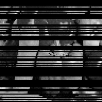
(a)	(b)
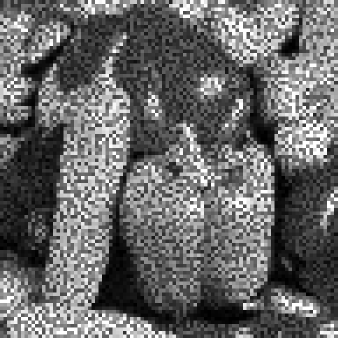
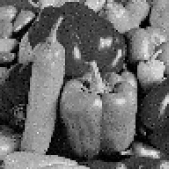
(c)	(d)

Figure 3: Experiment 2: (a) Original $\overline{x}$. (b) Observation $b$. (c) Observation $c$. (d) Recovery (all recoveries were visually indistinguishable).

Figure 4: Normalized error $20\log_{10}(\|\boldsymbol{x}_{n}-\boldsymbol{x}_{\infty}\|/\|\boldsymbol{x}_{0}-\boldsymbol{x}_{\infty}\|)$ (dB) versus epoch count in Experiment 2. Top: Algorithm A. The horizontal axis starts at 140 epochs to account for the auxiliary tasks (see a/). Bottom: Algorithm B. The computational load per epoch for Algorithm B was about twice that of Algorithm A.

References

• [1] A. Argyriou, R. Foygel, and N. Srebro, Sparse prediction with the $k$-support norm, Proc. Adv. Neural Inform. Process. Syst. Conf., vol. 25, pp. 1457–1465, 2012.
• [2] J.-F. Aujol and A. Chambolle, Dual norms and image decomposition models, Int. J. Comput. Vision, vol. 63, pp. 85–104, 2005.
• [3] F. Bach, R. Jenatton, J. Mairal, and G. Obozinski, Optimization with sparsity-inducing penalties, Found. Trends Machine Learn., vol. 4, pp. 1–106, 2012.
• [4] J. M. Bioucas-Dias, A. Plaza, N. Dobigeon, M. Parente, Q. Du, P. Gader, and J. Chanussot, Hyperspectral unmixing overview: Geometrical, statistical, and sparse regression-based approaches, IEEE J. Select. Topics Appl. Earth Observ. Remote Sensing, vol. 5, pp. 354–379, 2012.
• [5] S. Boyd, N. Parikh, E. Chu, B. Peleato, and J. Eckstein, Distributed optimization and statistical learning via the alternating direction method of multipliers, Found. Trends Machine Learn., vol. 3, pp. 1–122, 2010.
• [6] L. M. Briceño-Arias, G. Chierchia, E. Chouzenoux, and J.-C. Pesquet, A random block-coordinate Douglas–Rachford splitting method with low computational complexity for binary logistic regression, Comput. Optim. Appl., vol. 72, pp. 707–726, 2019.
• [7] A. Chambolle, M. J. Ehrhardt, P. Richtárik, and C.-B. Schönlieb, Stochastic primal-dual hybrid gradient algorithm with arbitrary sampling and imaging applications, SIAM J. Optim., vol. 28, pp. 2783–2808, 2018.
• [8] A. Chambolle and T. Pock, An introduction to continuous optimization for imaging, Acta Numer., vol. 25, pp. 161–319, 2016.
• [9] P. L. Combettes and J. Eckstein, Asynchronous block-iterative primal-dual decomposition methods for monotone inclusions, Math. Program. Ser. B, vol. 168, pp. 645–672, 2018.
• [10] P. L. Combettes and L. E. Glaudin, Proximal activation of smooth functions in splitting algorithms for convex image recovery, SIAM J. Imaging Sci., vol. 12, pp. 1905–1935, 2019.
• [11] P. L. Combettes and L. E. Glaudin, Solving composite fixed point problems with block updates, Adv. Nonlinear Anal., vol. 10, 2021.
• [12] P. L. Combettes, A. M. McDonald, C. A. Micchelli, and M. Pontil, Learning with optimal interpolation norms, Numer. Algorithms, vol. 81, pp. 695–717, 2019.
• [13] P. L. Combettes and C. L. Müller, Perspective maximum likelihood-type estimation via proximal decomposition, Electron. J. Stat., vol. 14, pp. 207–238, 2020.
• [14] P. L. Combettes and J.-C. Pesquet, Proximal splitting methods in signal processing, Fixed-Point Algorithms for Inverse Problems in Science and Engineering, pp. 185–212. Springer, 2011.
• [15] P. L. Combettes and J.-C. Pesquet, Stochastic quasi-Fejér block-coordinate fixed point iterations with random sweeping, SIAM J. Optim., vol. 25, pp. 1221–1248, 2015.
• [16] P. L. Combettes and J.-C. Pesquet, Fixed point strategies in data science, IEEE Trans. Signal Process., vol. 69, pp. 3878–3905, 2021.
• [17] J. Darbon and T. Meng, On decomposition models in imaging sciences and multi-time Hamilton–Jacobi partial differential equations, SIAM J. Imaging Sci., vol. 13, pp. 971–1014, 2020.
• [18] A. J. Defazio, T. S. Caetano, and J. Domke, Finito: A faster, permutable incremental gradient method for big data problems, Proc. Intl. Conf. Machine Learn., pp. 1125–1133, 2014.
• [19] R. Glowinski, S. J. Osher, and W. Yin (Eds.), Splitting Methods in Communication, Imaging, Science, and Engineering. Springer, 2016.
• [20] M. Hintermüller and G. Stadler, An infeasible primal-dual algorithm for total bounded variation-based inf-convolution-type image restoration, SIAM J. Sci. Comput., vol. 28, pp. 1–23, 2006.
• [21] L. Jacob, G. Obozinski, and J.-Ph. Vert, Group lasso with overlap and graph lasso, Proc. Int. Conf. Machine Learn., pp. 433–440, 2009.
• [22] P. R. Johnstone and J. Eckstein, Projective splitting with forward steps, Math. Program. Ser. A, published online 2020-09-30.
• [23] K. Mishchenko, F. Iutzeler, and J. Malick, A distributed flexible delay-tolerant proximal gradient algorithm, SIAM J. Optim., vol. 30, pp. 933–959, 2020.
• [24] J.-C. Pesquet and A. Repetti, A class of randomized primal-dual algorithms for distributed optimization, J. Nonlinear Convex Anal., vol. 16, pp. 2453–2490, 2015.
• [25] S. Salzo and S. Villa, Parallel random block-coordinate forward-backward algorithm: A unified convergence analysis, Math. Program. Ser. A, published online 2021-04-11.
• [26] M. Schmidt, N. Le Roux, and F. Bach, Minimizing finite sums with the stochastic average gradient, Math. Program. Ser. A, vol. 162, pp. 83–112, 2017.