Dynamic soliton-mean flow interaction with nonconvex flux

Abstract

The interaction of localised solitary waves with large-scale, time-varying dispersive mean flows subject to nonconvex flux is studied in the framework of the modified Korteweg-de Vries (mKdV) equation, a canonical model for nonlinear internal gravity wave propagation in stratified fluids. The principal feature of the studied interaction is that both the solitary wave and the large-scale mean flow—a rarefaction wave or a dispersive shock wave (undular bore)—are described by the same dispersive hydrodynamic equation. A recent theoretical and experimental study of this new type of dynamic soliton-mean flow interaction has revealed two main scenarios when the solitary wave either tunnels through the varying mean flow that connects two constant asymptotic states, or remains trapped inside it. While the previous work considered convex systems, in this paper it is demonstrated that the presence of a nonconvex hydrodynamic flux introduces significant modifications to the scenarios for transmission and trapping. A reduced set of Whitham modulation equations, termed the solitonic modulation system, is used to formulate a general, approximate mathematical framework for solitary wave-mean flow interaction with nonconvex flux. Solitary wave trapping is conveniently stated in terms of crossing characteristics for the solitonic system. Numerical simulations of the mKdV equation agree with the predictions of modulation theory. The developed theory draws upon general properties of dispersive hydrodynamic partial differential equations, not on the complete integrability of the mKdV equation. As such, the mathematical framework developed here enables application to other fluid dynamic contexts subject to nonconvex flux.

1 Introduction

The interaction of dispersive waves with slowly varying mean flows is a fundamental and canonical problem of fluid mechanics with important applications in geophysical fluid dynamics (see, e.g. [54, 6] and references therein). This multiscale problem is relevant for linear or weakly nonlinear wavepackets and large amplitude solitons—in this work, we do not distinguish between solitary waves and solitons. Traditionally, the mean flow involved in the interaction is either prescribed externally, e.g. an external current, or is induced by amplitude modulations of a nonlinear wave. A different class of wave-mean flow interactions has recently been identified in [52], where both the dynamic mean flow and the propagating localised soliton are described by the same dispersive hydrodynamic equation, a canonical example being the Korteweg-de Vries (KdV) equation. However, the evolution of the field $u(x,t)$ occurs on two well separated spatiotemporal scales, allowing for the distinct identification of waves and mean flows. A prototypical configuration of this (Fig. 1) is the propagation of a soliton through a dynamically evolving macroscopic flow, characterised by different asymptotic states $u\to u_{\pm}$ as $x\to\pm\infty$. We refer to such nonlinear wave interactions as soliton-mean flow interactions. The simplest mean flows are initiated by a monotone transition or step between $u_{-}$ and $u_{+}$, which asymptotically develops into either a rarefaction wave (RW) or a highly oscillatory dispersive shock wave (DSW) [24, 16]. While the former is slowly varying, the use of the term “mean flow” for the latter implies some averaging over rapid oscillations. We shall refer to the step problem for dispersive hydrodynamics as a dispersive Riemann problem.

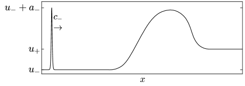
Figure 1: Representative initial configuration for soliton-mean flow interaction. The narrow soliton with amplitude $a_{-}$ on the uniform mean flow $\overline{u}_{-}$ transmits through the broad hydrodynamic flow if it reaches the uniform mean flow $\overline{u}_{+}$, otherwise it experiences trapping inside the mean flow. The mean flow generally exhibits expansion and compression waves.

Depending upon its initial position and amplitude, the soliton may “tunnel” or transmit through the large scale, expanding mean flow; otherwise, it remains trapped within the mean flow. Recent work has investigated the interaction between solitons and mean flows resulting from the evolution of an initial step. Both fluid conduit experiments and the theory for a rather general, single dispersive hydrodynamic conservation law were described in [52]. A generalisation of soliton-mean flow interaction to the bidirectional case for a pair of conservation laws described by the defocusing NLS equation was explored in [62]. Soliton-mean flow interaction in the focusing NLS equation was investigated in [5]. A similar problem involving the interaction of linear wavepackets with mean flows arising from the step problem in the KdV equation was studied using an analogous modulation theory framework in [9]. Aside from the focusing NLS case, for which mean flow evolution is described by an elliptic system of equations, and the present work, the models previously investigated in the context of soliton-mean flow interaction were limited to dispersive conservation laws with hyperbolic convex flux.

The focus of this work is the study of soliton-mean flow interaction when the governing dispersive hydrodynamics exhibit a nonconvex hydrodynamic flux. As we show, the presence of nonconvex flux, e.g. the cubic flux in the modified KdV (mKdV) equation or related Gardner equation, introduces significant modifications to the transmission and trapping scenarios realised in the KdV case. First of all, due to the nonconvex flux, the mKdV equation supports a much broader family of solitons and large-scale mean flow solutions than the KdV equation. In particular, it exhibits localised solutions in the form of exponentially decaying solitons of both polarities and, depending on the dispersion sign, kinks and algebraic solitons. The mKdV nonconvex mean flow features include undercompressive DSWs (an alternative interpretation of kinks), contact DSWs (CDSWs) and compound two-wave structures [37, 38, 14]. Here, we investigate how the solution features that arise due to nonconvex flux affect soliton-mean flow interactions. In particular, we show that soliton transmission for the defocusing mKdV equation can be accompanied by a soliton polarity change. In the focusing case, there is a soliton-mean flow interaction in which an exponential soliton is asymptotically transformed into a trapped algebraic soliton. These are just two examples of the rich catalogue of soliton-mean flow interactions we describe in this paper.

Key to the study of soliton-mean flow interaction is scale separation, whereby the characteristic length and time scales of the propagating soliton are much shorter than those of the mean flow. The rapidly oscillating structure of dispersive hydrodynamic flows motivates the use of multiscale asymptotic methods. Here, we will make extensive use of one such method known as Whitham modulation theory [65], which is based on a projection of the scalar dispersive hydrodynamics onto a three-parameter family of slowly varying periodic travelling wave solutions to the governing equation. The projection is achieved, equivalently, by averaging conservation laws, an averaged variational principle, or multiple scales perturbation methods. The dispersive hydrodynamics are then approximately described by a system of three first order quasilinear partial differential equations (PDEs)—the Whitham modulation equations—for the periodic travelling wave’s parameters such as the wave amplitude, the wavenumber and the period-mean. Within the framework of Whitham modulation theory, the original dispersive Riemann problem is posed as a special Riemann problem, sometimes called the Gurevich-Pitaevskii (GP) problem [24], for the modulation equations subject to piecewise constant initial data with a single discontinuity at the origin. Continuous, self-similar solutions of the GP problem describe RW and DSW mean flow modulations.

Classical DSW modulation theory has been developed for the KdV equation [24] and other “KdV-like” equations, both integrable and non-integrable [15, 16]. It is useful to identify this class of KdV-type equations, or classical, convex dispersive hydrodynamic equations, as those equations whose associated Whitham modulation equations are strictly hyperbolic and genuinely nonlinear. In this case, the generic solution of the GP problem is either a DSW or a RW. More broadly, even nonconvex equations such as mKdV can exhibit convex dispersive hydrodynamics for a restricted subset of modulation parameters in which the Whitham modulation equations remain strictly hyperbolic and genuinely nonlinear. Therefore, we shall call the DSWs generated within the framework of convex dispersive hydrodynamics convex DSWs.

It was shown in [52] that the interaction of a soliton with a RW is described by an exact, soliton limit reduction of the Whitham modulation system, which we call the solitonic modulation system. Two integrals or adiabatic invariants of the solitonic modulation system were identified that determine the amplitude and phase shift of the soliton when transmitted through the variable mean flow. The nonexistence of a transmitted soliton (zero or negative transmitted amplitude) signifies soliton trapping within the mean flow. The soliton-DSW transmission/trapping conditions were shown to be equivalent to those for the soliton-RW interaction by the fundamental property of hydrodynamic reciprocity of the modulation solution, which is related to time reversibility of the original dispersive hydrodynamics.

In this paper, we investigate the effects of a flux’s nonconvexity on the transmission and phase conditions. One of the main, general outcomes of our work is the identification of the condition for soliton trapping with the coalescence of characteristics of the solitonic modulation system, a signature of nonstrict hyperbolicity. Analysis of the solitonic modulation system for the mKdV equation shows that, in contrast to the convex case, the characteristic coalescence and, consequently, soliton trapping can occur even for nonzero soliton amplitude. This new type of soliton trapping is accompanied by the asymptotic transformation of a conventional, exponentially decaying soliton into an algebraic soliton of the mKdV equation. Another notable effect is the dynamic reversal of soliton polarity upon its transmission through a kink mean flow, which resembles but is different from the well-known soliton polarity reversal due to KdV soliton propagation in a variable medium caused for example, by internal wave propagation through variable fluid stratification and/or variable depth. Upon passage through a critical point where the coefficient for the quadratic flux vanishes, nonconvex mKdV/Gardner dynamics emerge [60, 50]. Modulation theory predicts a zero—or more accurately, vanishing in the zero dispersion limit—phase shift of soliton transmission through a nonconvex mean flow such as a kink or contact DSW. Although all concrete calculations and numerical simulations are performed for the mKdV equation, the developed solitonic modulation system framework for the analysis of nonconvex soliton-mean flow interactions is general and can be applied to other dispersive hydrodynamic equations with nonconvex flux, both integrable and non-integrable.

Perhaps the most prominent application of the present work is to internal waves in the ocean and atmosphere where solitons are known to arise and may interact with large scale mean flows modelled by the unidirectional mKdV and Gardner equations [35, 28, 22, 26, 2]. A more sophisticated nonconvex model describing long-wave potential-vorticity dynamics of coastal fronts was recently introduced in [34]. Fully nonlinear, bidirectional internal waves are described by nonconvex dispersive models such as the Miyata-Camassa-Choi system [56, 8] for fully nonlinear internal waves. Nonconvex dispersive dynamics modelled by the mKdV and Gardner equations also occur in the physics of multicomponent superfluids [31] and collisionless plasma [7, 58].

The structure of this paper is as follows. In Section 2 we introduce the notion and nomenclature of dispersive hydrodynamics, and provide a review of the effects of nonconvex hydrodynamic flux on mKdV solutions. In Section 3, we detail the general modulation theory framework for soliton-mean flow interaction problems, originally introduced in [52], and extend it to the case of nonconvex flux. Then, in Section 4, we narrow our focus to the modulation description of mKdV dispersive hydrodynamics and in Section 5 to the classification of mean flows realised in the mKdV regularisation of Riemann step data. In the next Section 6, we formulate the soliton-mean flow problem for mKdV and determine admissibility conditions for soliton transmission (tunnelling) through the mean flow. We then partition our classification of mKdV soliton-mean flow interaction into soliton-convex mean flow interactions (Section 7), soliton-nonconvex mean flow interactions (Section 8), and the special case of kink-mean flow interactions (Section 9). Finally, we generalise our analysis from convex mean flows generated by the GP problem to a much broader class of convex mean flows generated from slowly varying initial conditions. Throughout this paper, we confirm the predictions of our asymptotic analysis using numerical experiments with a spectral integrating factor Fourier method (described in Appendix B of [14]) in space and fourth order Runge-Kutta time integration. Discussion, conclusions and future outlooks are given in Section 11.

2 Nonconvex dispersive hydrodynamics

Dispersive hydrodynamics are modeled by hyperbolic conservation laws modified by dispersive terms [16]. We express a single one-dimensional dispersive hydrodynamic conservation law in the general form

$$u_{t}+f(u)_{x}=D[u]_{x},$$ (1)

where $f(u)\in C^{2}(\mathbb{R})$ is the hydrodynamic (or hyperbolic) flux function. The term $D[u]$ is an integro-differential operator acting on $u(x,t)$ that gives rise to a real-valued linear dispersion relation

$$\omega_{0}(k,\overline{u})=f^{\prime}(\overline{u})k+\Omega(k,\overline{u}),\quad k\in\mathbb{R}$$ (2)

for vanishingly small amplitude travelling wave solutions $\propto e^{i(kx-\omega_{0}t)}$ of the PDE (1) linearized about the constant solution $u(x,t)=\overline{u}\in\mathbb{R}$. We assume that $\Omega(k,\overline{u})=o(k)$ as $k\to 0$ and $\Omega_{kk}(k,\overline{u})$ is not identically zero in order to separate the long-wave hydrodynamic flux from short-wave dispersive effects. The field of dispersive hydrodynamics encompasses multiscale nonlinear wave solutions of initial and boundary value problems for eq. (1) (possibly with perturbations) in which at least two length and time scales play a prominent role: the oscillatory scale (e.g., the width of a soliton or the wavelength/period of a periodic travelling wave) and a longer, hydrodynamic scale (e.g., the slowly varying oscillatory amplitude of a wavepacket or DSW). One canonical dispersive hydrodynamic problem for eq. (1) is the so-called Gurevich-Pitaevskii (GP) problem [24] in which $u(x,0)$ for $x\in\mathbb{R}$ exhibits a sharp, monotone transition between two distinct far-field boundary conditions. The solution of the GP problem then describes the long-time asymptotic behaviour for more general initial data with distinct far-field equilibrium states.

When $f^{\prime\prime}(u)$ in (1) is sign definite, we say that the hydrodynamic flux—or just “flux” for short—is convex, not distinguishing between convex and concave associated with different signs. Similarly, when $\Omega_{kk}(k,\overline{u})$ in (2) is sign definite for $k>0$, we say that the dispersion is convex. A necessary condition for (1) to be a classical, convex dispersive hydrodynamic equation is the convexity of both the flux and the dispersion [16]. Consequently, when $f^{\prime\prime}$ or $\Omega_{kk}$ are sign indefinite, the dispersive hydrodynamics are nonconvex. In this paper, we focus on the nonconvex flux case and assume convex dispersion throughout.

Nonconvexity is known to introduce new types of dispersive hydrodynamic solutions. The simplest generic model of dispersive hydrodynamics with nonconvex flux is the modified Korteweg-de-Vries (mKdV) equation

$$u_{t}+(u^{3})_{x}=\mu u_{xxx}.$$ (3)

The mKdV equation with $\mu>0$ is often referred to as defocusing and with $\mu<0$ as focusing. The review [14] presents a full classification of mKdV solutions to the GP problem associated to the Riemann initial data

$$u(x,0)=\begin{cases}u_{-}&x<0\\ u_{+}&x>0\end{cases}$$ (4)

for both signs of $\mu$. Due to its cubic flux, the mKdV Riemann problem exhibits nonclassical solutions that were first studied in [7, 39, 53, 47, 46]. The full classification was carried out in [37, 38] within the framework of the Gardner equation that combines the quadratic and cubic fluxes of the KdV and mKdV equations, respectively. The classification is presented in Section (5); see Fig. 4.

The complete integrability of the mKdV equation was utilised in [44, 43, 20] to obtain detailed asymptotics of exact solutions to (3) with $\mu<0$ and step-like initial data for far-field asymptotic states satisfying $u_{-}>u_{+}>0$. The method of analysis is the formulation and asymptotic solution of a Riemann-Hilbert problem within the inverse scattering transform formalism.

The properties of the mKdV equation for $\mu>0$ and $\mu<0$ are very different with respect to the evolution of Riemann data (4). In addition to convex DSWs and RWs exhibited by both mKdV incarnations, there are new types of nonclassical, nonconvex solutions that do not exist for convex dispersive hydrodynamic equations and depend on the sign of $\mu$. These features occur for initial steps satisfying $u_{-}u_{+}<0$, i.e. when the initial data include the inflection point $u=0$ of the cubic flux $f(u)=u^{3}$. When $\mu>0$, monotonic, heteroclinic travelling wave solutions, commonly known as kinks, were identified in [41] as undercompressive DSWs analogous to discontinuous, undercompressive shock wave solutions in conservation law theory that do not satisfy the Lax entropy condition [48]. The solutions of the mKdV Riemann problem involving kinks were analyzed in [7] using the inverse scattering transform and in [47] using matched asymptotic expansions.

When $\mu<0$, a family of contact DSWs (CDSWs) exist whose modulation solution coincides with a nonstrictly hyperbolic double characteristic of the Whitham modulation system. Contact DSWs are analogous to contact discontinuities in conservation law theory that propagate with characteristic velocity [12]. Contact DSWs were first described in [53] as “sinusoidal undular bores”, then later as trigonometric bores which were studied in [46] using matched asymptotic expansions.

While convex DSWs are a continuous, two-parameter family of solutions to the GP problem depending on both $(u_{-},u_{+})$, undercompressive and contact DSWs are a continuous, one-parameter family of solutions. For mKdV (3), the undercompressive and CDSWs exhibit the additional restriction $u_{+}=-u_{-}$. As a result, undercompressive and contact DSWs resulting from the GP problem are typically accompanied by a convex RW or DSW in the form of a double wave structure. Representative numerical simulations for each type of solution to the mKdV GP problem are shown in Fig. 4. In the context of soliton interaction with dispersive hydrodynamic structures, we shall refer to solutions of the GP problem generally as mean flows. The DSW modulations in this context are further specified as DSW mean flows.

In addition to the already mentioned Gadner equation, which can be reduced to mKdV by a simple transformation, there are a number of dispersive PDEs modelling bidirectional flows in the nonconvex regime. These manifest as a coupled pair of dispersive hydrodynamic conservation laws whose dispersionless limit is not genuinely nonlinear for a subset of field values. Prominent examples of nonconvex flux for bidirectional flows include the Landau-Lifshitz equation modelling two-component Bose-Einstein condensates and thin, easy-plane ferromagnetic materials [31] and the Miyata-Camassa-Choi equations modelling two-layer, stratified fluids [18]. The GP problem for these equations includes double waves involving contact DSWs (Landau-Lifshitz equation) and undercompressive DSWs (Miyata-Camassa-Choi equation). Nonconvex mean flows have also been studied for variants of the nonlinear Schrödinger (NLS) equation including the defocusing complex mKdV equation [42], the derivative NLS equation [36], the discrete NLS equation from which mKdV can be derived [39], and NLS with self-steepening terms [33, 32], all of which include contact DSW solutions.

3 Modulation Theory for Soliton-Mean Interaction

We now review the general approach to the mathematical study of soliton-mean interaction via Whitham modulation theory [65]. This approach, termed solitonic dispersive hydrodynamics, was introduced in [52]. The key feature of solitonic dispersive hydrodynamics is that both the soliton and the mean flow are described by the same equation, albeit the variations of the wave field occur on disparate scales. This is in sharp contrast with the traditional wave-mean flow interaction setting where the mean flow is prescribed externally; see, e.g. [6]. We shall first follow the general description introduced in [52] for convex systems and then consider the implications of a nonconvex flux, not explored previously.

3.1 Solitonic modulation system

The analytical description of solitonic dispersive hydrodynamics is based on considering the soliton reduction of the Whitham modulation equations. Having the mKdV equation in mind, we present the general theory for the unidirectional, scalar case.

For a periodic travelling wave solution parametrised by three independent constants (as in the case of KdV or mKdV equations, third order PDEs), the modulation equations can be written in terms of the physical wave parameters: the mean flow $\bar{u}$, the amplitude $a$, and the wavenumber $k$. Allowing $\bar{u}$, $a$, $k$ to be slow functions of $x,t$, the requirement for the modulated periodic wave to be an asymptotic solution to the dispersive hydrodynamic equation (1) results in the quasilinear modulation system,

$${\bf u}_{t}+\mathrm{A}({\bf u}){\bf u}_{x}=0,$$ (5)

where ${\bf u}=(\bar{u},a,k)^{T}$ and $\mathrm{A}({\bf u})$ is a $3\times 3$ modulation matrix. We call the dispersive hydrodynamics convex if the associated Whitham modulation system (5) is strictly hyperbolic and genuinely nonlinear. If at least one of these conditions is violated, the system is nonconvex. Strict hyperbolicity requires that the eigenvalues $v_{i}({\bf u}),\ i=1,2,3$ of matrix $\mathrm{A}({\bf u})$ are real and distinct, $v_{1}<v_{2}<v_{3}$ for all admissible $\bf u$ in the admissible set

$${\bf u}\in\mathcal{A}=\left\{(\bar{u},a,k)^{T}~{}|~{}\bar{u}\in\mathbb{R},~{}a>0,~{}k\in\mathbb{R}\setminus\{0\}\right\}.$$ (6)

The genuine nonlinearity condition then reads $\nabla_{\bf u}v_{i}\cdot{\bf r}_{i}\neq 0,\ i=1,2,3$ for all ${\bf u}\in\mathcal{A}$, where ${\bf r}_{i}({\bf u})$ is the right eigenvector corresponding to the eigenvalue $v_{i}$ [45]. If the system is nonstrictly hyperbolic (the eigenvectors ${\bf r}_{i}$ span $\mathbb{R}^{3}$ but multiple eigenvalues are admissible), then it is not genuinely nonlinear either [12]. The converse is generally not true. Nevertheless, a nonconvex system can exhibit convex properties in a restricted domain of ${\bf u}\in\mathcal{D}\subset\mathcal{A}$.

The KdV-Whitham modulation system (5) is strictly hyperbolic and genuinely nonlinear for all admissible ${\bf u}\in\mathcal{A}$ [49], while for the mKdV equation, the properties of strict hyperbolicity and genuine nonlinearity depend on the sign of $\mu$ and on the range of initial Riemann data (4) [14].

An important ingredient for modulation theory is the equation for $k$ in (5). It has the universal form

$$k_{t}+[\omega(\bar{u},k,a)]_{x}=0,$$ (7)

known as the conservation of waves, where $\omega(\bar{u},k,a)$ is the travelling wave frequency.

Being a $3\times 3$ system, the quasi-linear equation (5) is generally not diagonalisable, although Riemann invariants are available for modulation systems associated with integrable dispersive hydrodynamics such as KdV or mKdV equations. It is important to stress that the general soliton-mean interaction theory developed in [52] is not reliant on the availability of Riemann invariants for or the integrability of the modulation system.

Soliton-mean interaction theory is based on the fundamental property of Whitham modulation systems that we postulate here in a general form and later explicitly justify for mKdV: in the $k\to 0$ soliton limit, the modulation system (5) admits the following exact reduction [23]:

$$\begin{bmatrix}\bar{u}\\ a\end{bmatrix}_{t}+\begin{bmatrix}f^{\prime}(\bar{u})&0\\ g(a,\bar{u})&c(a,\bar{u})\end{bmatrix}\begin{bmatrix}\bar{u}\\ a\end{bmatrix}_{x}=\begin{bmatrix}0\\ 0\end{bmatrix},$$ (8)

where $c(a,\bar{u})=\lim_{k\to 0}(\omega/k)$ is the soliton amplitude-speed relation for propagation on the background $\bar{u}$ and $g(a,\bar{u})$ is a coupling function that is system dependent. Equation (8) is called the solitonic modulation system.

The third modulation equation (7) is identically satisfied for $k=0$ while for $0<k\ll 1$, it assumes at leading order the form

$$k_{t}+[c(a,\bar{u})k]_{x}=0.$$ (9)

Equation (9) can be added to the solitonic modulation system (8) to give an approximate modulation system for a train of noninteracting solitons propagating on a variable mean flow. Equation (9) then signifies the conservation of the number of solitons in the train. We shall refer to the combined system (8) and (9) as the augmented solitonic modulation system. Note that a particular case of this system was derived in [21] for slowly varying soliton solutions of the variable coefficent KdV equation.

The soliton train interpretation of the modulation system (8) is instrumental for solitonic dispersive hydrodynamics as it enables the description of a single modulated soliton by treating the soliton amplitude $a(x,t)$ as a spatiotemporal field, in contrast to standard soliton perturbation theory where the soliton’s parameters evolve temporally along its trajectory in the $x,t$-plane; see, e.g. [40]. Additionally, as we will show, the introduction of the fictitious wavenumber field $k(x,t)$ for a single soliton enables the determination of the soliton phase shift due to interaction with the mean flow.

The characteristic velocities of the system (8) are $f^{\prime}(\bar{u})$ and $c(a,\bar{u})$. The right eigenvectors ${\bf r}_{1,2}$ of the Jacobian matrix in (8) for each characteristic velocity are

$$v_{1}=f^{\prime}(\bar{u}),\qquad {\bf r}_{1}=\begin{bmatrix}f^{\prime}-c\\ g\end{bmatrix},$$ (10)

$$v_{2}=c(a,\bar{u}),\qquad {\bf r}_{2}=\begin{bmatrix}0\\ 1\end{bmatrix}.$$ (11)

Thus, the system (8) is strictly hyperbolic if $f^{\prime}\neq c$ for all $(\bar{u},a)\in\mathcal{A}_{0}$, where

$$\mathcal{A}_{0}=\mathbb{R}\times(0,\infty)$$ (12)

is the set of admissible states. The system (8) is genuinely nonlinear in the $j$th characteristic field if $\nabla v_{j}\cdot{\bf r}_{j}\neq 0$ for all $(\bar{u},a)\in\mathcal{A}_{0}$. For the first characteristic field,

$$\nabla f^{\prime}(\bar{u})\cdot{\bf r}_{1}\neq 0\implies f^{\prime\prime}(\bar{u})(f^{\prime}(\bar{u})-c(a,\bar{u}))\neq 0,$$ (13)

which holds, provided the characteristic velocities are distinct (strict hyperbolicity) and the flux $f$ of the original scalar evolution equation (1) is convex. Thus, when two characteristic velocities merge (nonstrict hyperbolicity), the corresponding characteristic field is not genuinely nonlinear.

The genuine nonlinearity of the second characteristic field requires

$$\nabla c(a,\bar{u})\cdot{\bf r}_{2}\neq 0\quad\implies c_{a}(a,\bar{u})\neq 0.$$ (14)

To summarise, the quasi-linear system (8) is strictly hyperbolic when $f^{\prime}(\bar{u})\neq c(a,\bar{u})$ and is genuinely nonlinear when additionally $f^{\prime\prime}(\bar{u})\neq 0$ and $c_{a}(a,\bar{u})\neq 0$ for all $(\bar{u},a)\in\mathbb{R}\times(0,\infty)$. Negation of any of these three conditions gives rise to nonconvex solitonic dispersive hydrodynamics.

Since the exact soliton reduction (8) is a $2\times 2$ quasi-linear hyperbolic system, it can be reduced to Riemann invariant form. We refer to the mean flow $\bar{u}$ as the “hydrodynamic” Riemann invariant and the other is found by integrating the differential form $g\,\mathrm{d}\bar{u}+(c-f^{\prime})\,\mathrm{d}a$ provided $c\neq f^{\prime}$ [65]. Denoting the second, “solitonic” Riemann invariant as $q=q(a,\bar{u})$, the diagonalised system can be written as

$$\begin{bmatrix}\bar{u}\\ q\end{bmatrix}_{t}+\begin{bmatrix}f^{\prime}(\bar{u})&0\\ 0&C(q,\bar{u})\end{bmatrix}\begin{bmatrix}\bar{u}\\ q\end{bmatrix}_{x}=\begin{bmatrix}0\\ 0\end{bmatrix},$$ (15)

where $C\big{(}q(a,\bar{u}),\bar{u}\big{)}\equiv c(a,\bar{u})$. In terms of the diagonal system (15), the condition of strict hyperbolicity reads $f^{\prime}(\bar{u})\neq C(q,\bar{u})$ and the conditions of genuine nonlinearity of the first and second characteristic field are written respectively as

$$f^{\prime\prime}(\bar{u})\neq 0,\quad\hbox{and}\quad C_{q}\neq 0.$$ (16)

It is important to stress that the existence of the solitonic Riemann invariant $q$ is not reliant on the diagonalisability of the full quasi-linear system (5) in Riemann invariants. In fact, as was shown in [15], this Riemann invariant can be obtained directly, as the integral $q=Q(\tilde{k},\bar{u})=const$ on $\mathrm{d}x/\mathrm{d}t=C$, of the following characteristic ODE

$$\frac{\mathrm{d}\tilde{k}}{d\bar{u}}=\frac{\partial_{\bar{u}}\tilde{\omega}_{0}}{f^{\prime}(\bar{u})-\partial_{\tilde{k}}\tilde{\omega}_{0}},$$ (17)

where $\tilde{k}$ and $\tilde{\omega}_{0}$ are called the conjugate wavenumber and conjugate frequency, respectively. They are defined in terms of the soliton amplitude-speed relation $c(a,\bar{u})$ and the linear dispersion relation (2) $\omega_{0}(k,\bar{u})$ by

$$\tilde{\omega}_{0}(\tilde{k},\bar{u})=-i\omega_{0}(i\tilde{k},\bar{u});\quad c(a,\bar{u})=\frac{\tilde{\omega}_{0}}{\tilde{k}}.$$ (18)

We note that the Riemann invariant $q=Q(\tilde{k},\bar{u})$ is not defined uniquely, as any smooth function of a Riemann invariant is also a Riemann invariant. In the case of convex systems, a convenient normalisation is suggested by the requirement to maintain strict hyperbolicity of the solitonic system in the limit of vanishing amplitude where the long-wave speed $f^{\prime}(\bar{u})$ and soliton speed $c(a,\bar{u})$ must coincide. The variable $\tilde{k}$ can be identified as an amplitude-type variable [15], so that $\tilde{k}=0\Longleftrightarrow a=0$, and require that the hydrodynamic and solitonic Riemann invariants coincide when $\tilde{k}\to 0$, i.e. $Q(0,\bar{u})=\bar{u}$. As a result, the system (15) reduces to a single hyperbolic equation $\bar{u}_{t}+f^{\prime}(\bar{u})\bar{u}_{x}=0$. The situation is different for nonconvex systems, where two or more distinct Riemann invariants associated with the same characteristic speed may exist. For example, for cubic flux $f(\bar{u})=\bar{u}^{3}$, the mean flow equation $\bar{u}_{t}+3\bar{u}^{2}\bar{u}_{x}=0$ is invariant with respect to the transformation $\bar{u}\to-\bar{u}$ so another possible normalization is $Q(0,\bar{u})=-\bar{u}$. To avoid ambiguity, we will be using the normalization

$$Q(0,\bar{u})=\bar{u}$$ (19)

for the initial configuration. For the case of a general nonconvex flux, we assumed, without loss of generality, that it satisfies $f^{\prime\prime}(0)=0$. Then, if the solution curve crosses $\bar{u}=0$, the normalisation of the Riemann invariant should be changed to $Q(0,\bar{u})=-\bar{u}$ across this point to maintain smoothness of $Q$.

The two Riemann invariants $\bar{u}$ and $q$ for the $2\times 2$ system (15) are also Riemann invariants for the $3\times 3$ augmented solitonic modulation system (15) and (9). But the latter quasi-linear system is not hyperbolic because its corresponding Jacobian matrix is deficient, with just two eigenvalues and two linearly independent eigenvectors. Nevertheless, it has another hyperbolic subsystem, in addition to (15), which is obtained by setting $q\equiv q_{0}$ constant, as will be the case for the soliton-mean flow interaction problems we consider. Then the remaining simple wave equation $\bar{u}_{t}+f(\bar{u})_{x}=0$, together with the approximate equation (9), where we replace $c(a,\bar{u})$ with $C(q_{0},\bar{u})$, form a hyperbolic subsystem. Equation (9) is diagonalised by the quantity $kp(q_{0},\bar{u})$, where

$$p(q_{0},\bar{u})=\exp\left(-\int_{\bar{u}_{0}}^{\bar{u}}\frac{C_{u}(q_{0},u)}{f^{\prime}(u)-C(q_{0},u)}\mathrm{d}u\right),\quad\bar{u}_{0}\in\mathbb{R}.$$ (20)

In other words, if $q=q_{0}$ is constant, we can use

$$(kp)_{t}+C(q_{0},\bar{u})(kp)_{x}=0$$ (21)

instead of (9). The quantities $q$ and $kp$ have been identified in [52] as adiabatic invariants of soliton-mean flow interaction.

3.2 Soliton-mean interaction

Solutions to the solitonic modulation system can now be sought subject to an initial mean flow $\bar{u}(x,0)=\bar{u}_{0}(x)$ and an initial soliton with amplitude $a_{0}$ located at $x=x_{0}$. However, we need an initial amplitude and wavenumber field $a(x,0)$, $k(x,0)$ defined for all $x$. This is obtained by invoking the soliton train description and asserting that the required solution of the augmented solitonic system (8), (9) is a simple wave (to be justified), meaning all but one Riemann invariant are constant. The nonconstant Riemann invariant is $\bar{u}$, in order to satisfy the initial condition. Then $a(x,0)$ is selected to maintain constant $q$:

$$q\big{(}a(x,0),\bar{u}_{0}(x)\big{)}=q_{0}\equiv q\big{(}a_{0},\bar{u}_{0}(x_{0})\big{)}.$$ (22)

Since $q$ constant is a solution, this reduces the augmented solitonic modulation system to the hyperbolic subsystem consisting of two diagonalised equations for $\bar{u}$ and $kp(q_{0},\bar{u})$. In order to define the initial wavenumber field $k(x,0)$, we set the latter Riemann invariant to also be constant

$$k(x,0)=k_{0}\frac{p_{0}}{p\big{(}q_{0},\bar{u}_{0}(x)\big{)}},$$ (23)

where $p_{0}\equiv p\big{(}q_{0},\bar{u}_{0}(x_{0})\big{)}$ and $k_{0}\equiv k(x_{0},0)\ll 1$ is a small, positive quantity whose particular value is not important for our consideration since we assume the limit $k_{0}\to 0$ in the soliton number conservation equation (9), and, therefore in (21).

The soliton-mean interaction problem can now be formulated and solved. Given the initial mean flow profile $\bar{u}(x,0)=\bar{u}_{0}(x)$, the soliton amplitude $a_{0}$ and location $x_{0}$, $\bar{u}(x,t)$ is the simple wave solution

$$x-f^{\prime}(\bar{u})t=H(\bar{u}),\quad H=u_{0}^{-1}$$ (24)

and the soliton amplitude and wavenumber fields satisfy

$$q(a,\bar{u})=q_{0},\quad k=k_{0}\frac{p_{0}}{p(q_{0},\bar{u})}.$$ (25)

We will focus our analysis on a generalised GP problem, in which initial conditions for the mean flow are given as in the original Riemann problem (4)

$$\bar{u}(x,0)=\left\{\begin{array}[]{ll}u_{-},&x<0,\\ u_{+},&x>0,\end{array}\right.$$ (26)

and the amplitude and wavenumber fields exhibit step variations

$$a(x,0)=\begin{cases}a_{-}&x<0\\ a_{+}&x>0\end{cases},\qquad k(x,0)=\begin{cases}k_{-}&x<0\\ k_{+}&x>0.\end{cases}$$ (27)

A sketch illustrating the generalised GP problem is shown in Fig. 2

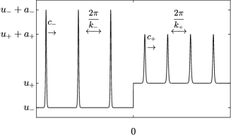
Figure 2: Sketch of the generalised GP problem.

Depending on the initial location $x_{0}$ of the soliton relative to the mean flow discontinuity at $x=0$, either the left $(a_{-},k_{-})$ or right $(a_{+},k_{+})$ part of the initial wave field $a(x,0),k(x,0)$ is prescribed with the other part to be determined as described below.

Due to the scaling invariance of both the quasilinear solitonic modulation system (8), (9) and the step initial data (26), (27), the soliton-mean interaction problem is solved by a simple wave solution of the Riemann problem, thus justifying the constant Riemann invariant assumption for $q$ and $kp$ expressed by equations (22), (23). Therefore, the amplitude and wavenumber fields in the soliton-mean flow interaction must satisfy (25), yielding the relations between admissible values of $a_{\pm}$ and $k_{\pm}$ in (27). These are formulated as transmission and phase conditions:

$$q(a_{-},u_{-}) =q(a_{+},u_{+}),$$ (28)

$$k_{-}p(q_{0},u_{-}) =k_{+}p(q_{0},u_{+}),$$ (29)

where $p(q,\bar{u})$ is defined by (20). It is important to stress that the existence of the simple wave solution leading to the conditions in eqs. (28) and (29) requires convexity (genuine nonlinearity) of the characteristic field (10) along the integral curve so that the conditions (13) are not violated.

In the context of a single soliton interacting with a varying mean flow connecting two equilibrium states $\bar{u}=u_{-}$ and $\bar{u}=u_{+}$, the conditions (28) and (29) should be interpreted as follows. The initial discontinuity (26) initiates the varying mean flow that is generally confined to the bounded, expanding region $s_{-}t<x<s_{+}t$. There is an exception to this for the undercompressive DSW mean flow, which is a nonexpanding travelling wave and requires a separate treatment. Then two basic scenarios of soliton-mean interaction can be realised that we describe by assuming positive polarity of the propagating soliton. The generalisation to negative polarity (dark) solitons is straightforward.

(i) Forward (left to right) transmission/trapping.

Assuming that the soliton with amplitude $a_{-}>0$ is initially placed at $x_{0}=x_{-}<0$ on the left, background mean flow state $\bar{u}=u_{-}$, then if the soliton velocity satisfies $c(a_{-},u_{-})>s_{-}$, soliton-mean flow interaction occurs for times $t>t_{1}=|x_{-}/(c(a_{-},u_{-})-s_{-})|$. As a result, the soliton either (a) gets transmitted (tunnels) through the variable mean flow and emerges on the right state $\bar{u}=u_{+}$ with the new amplitude $a_{+}>0$ determined by the condition (28) or (b) gets trapped within the variable mean flow. The trapping occurs if the transmitted soliton amplitude defined by (28) is negative or zero, $a_{+}\leq 0$.

For this case of forward transmission, the trajectory of the soliton post interaction is given by $x=c(a_{+},u_{+})t+x_{+}$, where generally $x_{+}\neq x_{-}$. This implies that soliton-mean flow transmission is accompanied by both an amplitude change and a soliton phase shift $\Delta=x_{+}-x_{-}$, which can be determined from the condition (29). To relate the $x$-intercepts $x_{\pm}$ of the soliton characteristic pre and post mean flow interaction we note that the conservation of the number of solitons in the fictitious modulated train of non-interacting solitons implies

$$k_{-}x_{-}=k_{+}x_{+}.$$ (30)

Given $x_{-}$, only the ratio of $k_{+}/k_{-}$ is needed to determine $x_{+}$, so, by virtue of the linear relationship between $k_{+}$ and $k_{-}$, the particular value of $k_{-}$ in (25) is irrelevant. The soliton phase shift $\Delta=x_{+}-x_{-}$ due to interaction with the mean flow is then given by

$$\frac{\Delta}{x_{-}}=\left(\frac{k_{-}}{k_{+}}-1\right)=\left(\frac{p_{+}}{p_{-}}-1\right),$$ (31)

where we have used the shorthand notation $p_{\pm}\equiv p(q_{0},u_{\pm})$.

(ii)  Backward (right to left) transmission/trapping.

If the soliton with amplitude $a_{+}$ is initially placed at $x_{0}=x_{+}>0$ on the right background $\bar{u}=u_{+}$ and $c(a_{+},u_{+})<s_{+}$, then soliton-mean flow interaction occurs for times $t>t_{2}=x_{+}/(s_{+}-c(a_{+},u_{+}))$. If the soliton eventually emerges from mean flow interaction onto the opposite constant background $\bar{u}=u_{-}$, its amplitude $a_{-}>0$ and phase shift $\Delta=x_{-}-x_{+}=x_{+}(p_{-}/p_{+}-1)$ are determined by the same transmission and phase conditions (28), (29). Otherwise, if the transmitted amplitude $a_{-}\leq 0$, the soliton remains trapped within the mean flow.

The generalisation to negative (dark) soliton interaction with mean flow is straightforward. For this, it is convenient to introduce a signed amplitude $a$, which enables the representation of both bright $a>0$ and dark $a<0$ solitons. Assuming negative initial amplitude $a_{\pm}<0$, forward/backward transmission requires that the transmitted amplitude $a_{\mp}$ maintains the same, negative, sign. Generally, the condition $a_{+}a_{-}>0$ is the sufficient condition for transmission in both bright and dark soliton cases. Its negation implies trapping.

In all cases of forward/backward transmission/trapping, the soliton trajectory for $t>0$ is given by the characteristic,

$$\frac{\mathrm{d}x}{\mathrm{d}t}=c(a(x,t),\bar{u}(x,t)),\qquad x(0)=x_{0},$$ (32)

where $|x_{0}|\gg 1$ so that the soliton is initially well-separated from the initial step in the mean flow at $x=0$.

In the present work, we consider the implications of a nonconvex solitonic modulation system (8) on the above soliton transmission and trapping scenarios. As described in Section 3.1, nonconvexity enters when strict hyperbolicity and/or genuine nonlinearity is lost via one of the three conditions: $f^{\prime\prime}(\bar{u})=0$, $f^{\prime}(\bar{u})=c(a,\bar{u})$, or $c_{a}(a,\bar{u})=0$ for any $(\bar{u},a)\in\mathcal{A}_{0}$.

In [52], positivity of the transmitted amplitude (one of $a_{\pm}$) was proposed as a necessary and sufficient condition for bright soliton tunnelling to occur through a mean flow for convex dispersive hydrodynamics. In fact, this condition coincides with a less restrictive definition of strict hyperbolicity for (8) where $a=0$ is included in the set of admissible states $\mathcal{A}_{0}^{\prime}=\mathbb{R}\times[0,\infty)$. Generally, the soliton speed coincides with the long wave speed when its amplitude vanishes, $c(0,\bar{u})=f^{\prime}(\bar{u})$, which signifies the onset of soliton trapping. Within the context of Whitham modulation theory, states in which $a=0$ or $k=0$ are not considered admissible when assessing strict hyperbolicity and genuine nonlinearity of the modulation equations because they coincide with a degeneracy in which the number of modulation equations is reduced; see, e.g., [49, 4]. We will utilise the traditional definition in which $a=0$ is not included in the set of admissible states (12).

In the more general nonconvex case, we find that in order for the soliton to tunnel through the mean flow, we must require the additional condition that the modulation system (8) remain strictly hyperbolic along the entire soliton trajectory for all admissible states $(\bar{u},a)\in\mathcal{A}_{0}$. If the characteristic speeds $f^{\prime}(\bar{u})$ and $c(a,\bar{u})$ coincide for nonzero $a$, then strict hyperbolicity is lost and the soliton is trapped inside the mean flow. If the speeds remain separated, the soliton amplitude on the transmitted side is non-zero and the phase shift is well-defined according to (29). In summary, the necessary and sufficient conditions for tunnelling in a nonconvex solitonic modulation system (15) with initial data (26), (27) is

$$q(a_{-},u_{-})=q(a_{+},u_{+}),\quad a_{+}a_{-}>0,\quad f^{\prime}(\bar{u}(x,t))\neq c(a(x,t),\bar{u}(x,t)),$$ (33)

where $x=x(t)$ is the characteristic (32) and $t\geq 0$.

3.3 Hydrodynamic reciprocity

So far, we have assumed that the mean flow satisfies the simple wave equation $\bar{u}_{t}+f^{\prime}(\bar{u})\bar{u}_{x}=0$. For step initial data (26), the only candidate continuous solution is a RW

$$\bar{u}(x,t)=\begin{cases}u_{-}&x<f^{\prime}(u_{-})t,\\ (f^{\prime})^{-1}(x/t)&f^{\prime}(u_{-})t<x<f^{\prime}(u_{+})t,\\ u_{+}&f^{\prime}(u_{+})t<x.\end{cases}$$ (34)

so long as the admissibility criterion $f^{\prime}(u_{-})<f^{\prime}(u_{+})$ holds, corresponding to expansive initial data. As will be shown in the next section, there is a much richer variety of dispersive mean flows generated by the mKdV GP problem when the initial data is compressive. Thus, we need soliton-mean flow modulation theory to be flexible enough to accommodate a wide class of mean flows.

The solitonic modulation equations (8), (9) directly apply for expansive mean flow initial data, yielding a description of soliton-RW interaction. For compressive initial data (26), rather than form a discontinuous shock solution, a DSW is formed that occupies the space-time region $A\subset\mathbb{R}\times(0,\infty)$ where the solution is described by the full system of Whitham modulation equations for a slowly varying nonlinear periodic wave. As a result, the Riemann invariant $q$ and secondary invariant $kp$ of the augmented solitonic system (8), (9) are not conserved in $A$, and our arguments leading to the transmission and phase conditions (28), (29) do not apply to the soliton interaction with the DSW mean flow.

To address this, we invoke an important property of the dispersive conservation law (1): time reversibility. A consequence of time reversibility is the continuity of the modulation solution for all $(x,t)\in\mathbb{R}^{2}$. For compressive data, we consider the solution for $t<0$ that consists of a simple wave described by (34), i.e., the expansive mean flow case. Then, since $q$ and $kp$ are constant for all $x\in\mathbb{R}$ and $t<0$, they remain constant by continuity for $(x,t)$ in the complement of $A$, outside of the oscillatory region, where the augmented solitonic system (8), (9) remains valid. Note that for the Riemann data (26), (27), the solution remains continuous outside $\mathbb{R}^{2}\setminus\{(0,0)\}$, which is justified by taking the limit of smooth solutions. This property was called hydrodynamic reciprocity in [52] and has been used previously in the characterization of DSWs for a single or pair of dispersive hydrodynamic conservation laws [15]. Since the transmission and phase conditions (28), (29) hold outside the oscillatory region, hydrodynamic reciprocity allows us to predict the transmitted amplitude and phase shift $\Delta$ of a soliton interacting with DSW mean flows entirely within the framework of the augmented solitonic modulation system (8), (9).

The details of the modulation dynamics for the soliton within the interior of the oscillatory region $A$ can, in principle, be described by a degenerate two-phase solution (see [19] for multiphase modulation theory of the KdV equation). However, as we will show, this rather technical approach can be partially, approximately circumvented by replacing $f(\bar{u})$ in the characteristic equation (17) by an appropriate choice of the mean flow variation and effectively defining a new adiabatic invariant $q$ holding within $A$.

4 Modified Korteweg–de Vries equation: travelling wave solutions and modulation equations

As the simplest example of dispersive hydrodynamics with nonconvex flux, we study the mKdV equation (3). The mean flow behaviours that arise when solving (3) subject to (26) depend on the sign of the dispersive term $\text{sgn}(\mu)$. The mKdV hyperbolic flux $f(u)=u^{3}$ exhibits the inflection point $f^{\prime\prime}(0)=0$ so that nonconvexity affects the solutions whenever the initial data contain an open interval including the point $u=0$. For either sign of $\mu$, the mKdV equation allows for solitons of both polarities by the symmetry $u\to-u$. The linear dispersion relation is

$$\omega_{0}=3\bar{u}^{2}k+\mu k^{3}.$$ (35)

In what follows, we present a compendium of the results from [14] necessary for the development in this paper.

4.1 Travelling wave solutions

The mKdV travelling wave solutions $u=u(\eta)$, $\eta=\frac{x-Ut}{\sqrt{2|\mu|}}$ are described by the ODE

$$(u_{\eta})^{2}=\text{sgn}(\mu)(u-u_{1})(u-u_{2})(u-u_{3})(u-u_{4})\equiv Q(u),$$ (36)

subject to the constraint $\sum_{i=1}^{4}u_{i}=0$ and ordering of the roots $u_{1}\leq u_{2}\leq u_{3}\leq u_{4}$. We only consider the modulationally stable case in which all roots are real. The phase velocity $U$ is given by

$$U=-\frac{1}{2}(u_{1}u_{2}+u_{1}u_{3}+u_{1}u_{4}+u_{2}u_{3}+u_{2}u_{4}+u_{3}u_{4}).$$ (37)

Equation (36) is a nonlinear oscillator equation in the potential $-Q(u)$. Figure 3 shows representative potential curves $Q(u)$ for both signs of the dispersion coefficient $\mu$. Travelling wave solutions exist in the regions where $Q(u)>0$ (shaded regions) and can be obtained by integrating (36) in terms of Jacobi elliptic functions. The cases $\mu<0$ and $\mu>0$ are treated separately.

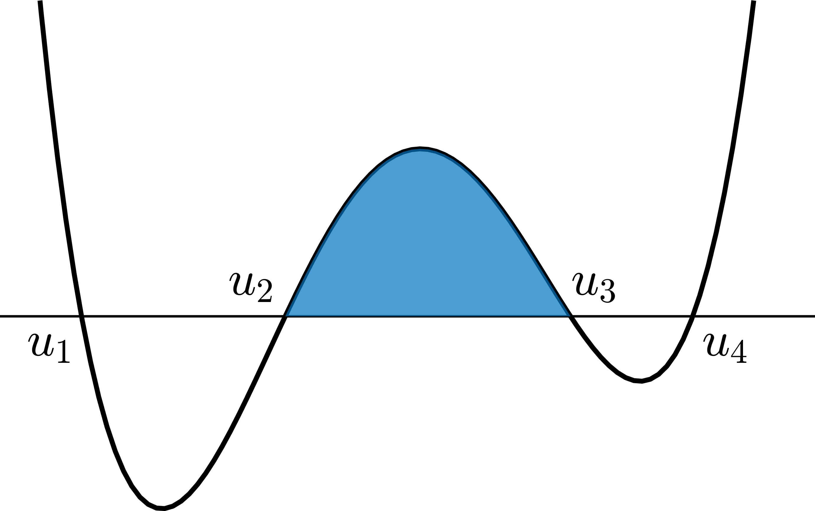
(a) $\mu>0$

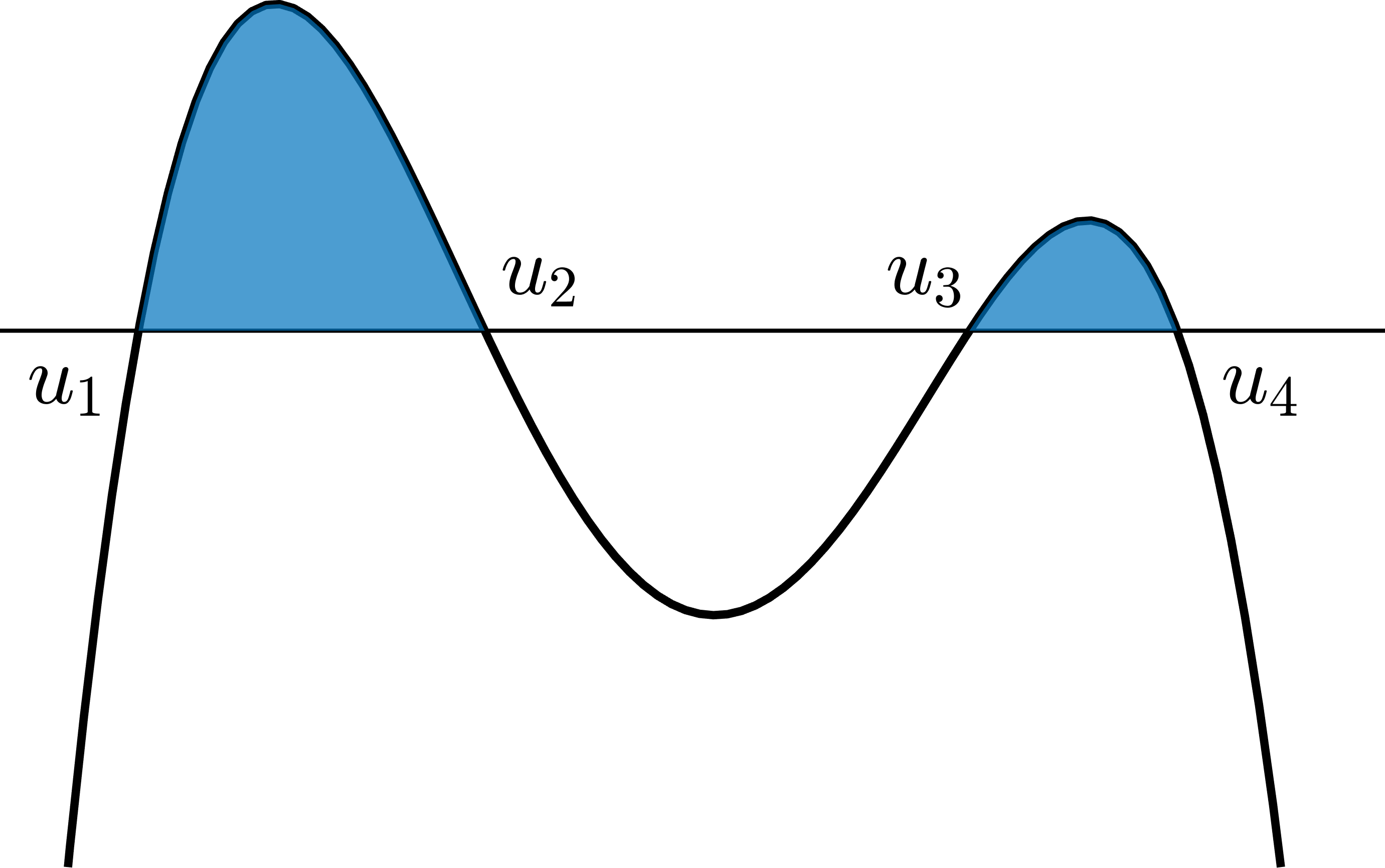
(b) $\mu<0$

Figure 3: Potential curve $Q(u)$ of the nonlinear oscillator equation (36). Travelling wave solutions exist in the shaded regions.

(i)  For $\mu>0$, the travelling wave solution is expressed in terms of Jacobi elliptic functions as

$$u=u_{2}+\frac{(u_{3}-u_{2})\text{cn}^{2}(\theta,m)}{1-\frac{u_{3}-u_{2}}{u_{4}-u_{2}}\text{sn}^{2}(\theta,m)}.$$ (38)

with $\theta=\sqrt{(u_{3}-u_{1})(u_{4}-u_{2})}\eta$ and modulus $m=m_{+}=\frac{(u_{3}-u_{2})(u_{4}-u_{1})}{(u_{4}-u_{2})(u_{3}-u_{1})}$. The wavenumber of the travelling wave is given by

$$k=\frac{\pi\sqrt{(u_{3}-u_{1})(u_{4}-u_{2})}}{2K(m)\sqrt{2|\mu|}}.$$ (39)

When $u_{2}\to u_{1}$ ($m_{+}\to 1$), the solution becomes a bright (positive polarity) soliton with amplitude $a=u_{3}-u_{1}$, mean background $\bar{u}=u_{1}<0$,

$$u=u_{1}+\frac{u_{3}-u_{1}}{\cosh^{2}\theta-\frac{u_{3}-u_{1}}{u_{4}-u_{1}}\sinh^{2}\theta},$$ (40)

which travels with the velocity $U=c_{+}$

$$c_{+}(a,\bar{u})=\frac{1}{2}a^{2}+2a\bar{u}+3\bar{u}^{2}.$$ (41)

Due to the root ordering, these bright solitons exist only for a certain range of positive amplitudes and a negative background, given by the constraint

$$0<a<-2\bar{u}.$$ (42)

Dark (negative polarity) soliton solutions occur when $u_{3}\to u_{4}$ instead. In this case, $\bar{u}=u_{4}>0$, $a=u_{4}-u_{2}>0$ and the soliton velocity $U=c_{-}$

$$c_{-}(a,\bar{u})=\frac{1}{2}a^{2}-2a\bar{u}+3\bar{u}^{2}.$$ (43)

with negative amplitudes $a$ satisfying

$$-2\bar{u}<a<0.$$ (44)

When $u_{2}\to u_{1}$ and additionally, $u_{3}\to u_{4}$, the travelling wave becomes a kink,

$$u=\pm\bar{u}\tanh(\bar{u}\eta),$$ (45)

a heteroclinic smooth transition connecting two equilibria $\bar{u}=u_{1}<0$ and $-\bar{u}=u_{4}>0$ (note that the constraint $\sum u_{j}=0$ becomes $u_{4}+u_{1}=0$ in this limit) and travelling with speed $U=\bar{u}^{2}$, which matches the classical shock speed determined by the Rankine-Hugoniot condition.

(ii)  For $\mu<0$, travelling wave solutions can occur between $u_{1}$ and $u_{2}$ or between $u_{3}$ and $u_{4}$. Between $u_{3}$ and $u_{4}$, the travelling wave solution is

$$u=u_{3}+\frac{(u_{4}-u_{3})\text{cn}^{2}(\theta,m)}{1+\frac{u_{4}-u_{3}}{u_{3}-u_{1}}\text{sn}^{2}(\theta,m)},$$ (46)

with $m=m_{-}=\frac{(u_{4}-u_{3})(u_{2}-u_{1})}{(u_{4}-u_{2})(u_{3}-u_{1})}$. The wavenumber is given by the same formula (40). When $u_{3}\to u_{2}$ ($m_{-}\to 1$) the solution becomes a bright exponential soliton with amplitude $a=u_{4}-u_{2}$ and background $\bar{u}=u_{2}$

$$u=u_{2}+\frac{u_{4}-u_{2}}{\cosh^{2}\theta+\frac{u_{4}-u_{2}}{u_{2}-u_{1}}\sinh^{2}\theta}.$$ (47)

This soliton solution travels according to the same soliton amplitude-speed relation (53) as in the case $\mu>0$. Due to the root ordering, valid bright soliton amplitudes for the solution to exist are given by

$$a>\max(0,-4\bar{u}),$$ (48)

with no constraint on the background $\bar{u}$.

For $\mu<0$, there is a special type of travelling wave solution expressible in terms of trigonometric functions. Again, these solutions occur either between $u_{1}$ and $u_{2}$ or between $u_{3}$ and $u_{4}$ but under the additional constraint that $u_{3}=u_{4}$ in the first case and $u_{1}=u_{2}$ in the second case. For $u_{3}\leq u\leq u_{4}$, $u_{1}=u_{2}$ the solution is given by

$$u=u_{3}+\frac{u_{4}-u_{3}}{1+\frac{u_{4}-u_{1}}{u_{3}-u_{1}}\tan^{2}\theta},$$ (49)

The nonlinear trigonometric solution (49) has no analogue in KdV theory. When $u_{3}\to u_{2}=u_{1}\equiv\bar{u}$, the solution (49) becomes an algebraic bright soliton described by

$$u=u_{1}+\frac{u_{4}-u_{1}}{1+(u_{4}-u_{1})^{2}\eta^{2}/4},$$ (50)

with amplitude $a=u_{4}-u_{1}=-4\bar{u}$ and travelling at speed $U=3u_{1}^{2}=3\bar{u}^{2}$, which is the characteristic speed of the dispersionless mKdV equation. Dark algebraic solitons can be obtained by the transformation (51) below.

The solution oscillating between $u_{1}$ and $u_{2}$, can be obtained by applying the invariant transformation

$$u\to-u,\qquad u_{i}\to-u_{5-i},\qquad i=1,2,3,4.$$ (51)

In this region, both the exponential and algebraic soliton solutions have negative polarity with amplitude $a=u_{3}-u_{1}$ and background $\bar{u}=u_{3}$ satisfying

$$a<\min(0,-4\bar{u}).$$ (52)

In both cases, the soliton amplitude-speed relation is given by (43). Heteroclinic kink solutions of mKdV do not exist if $\mu<0$.

Summarising, the mKdV equation differs from the KdV equation in that it supports solitons of both polarities for either sign of the dispersion $\mu$. For $\mu>0$, bright soliton solutions occur when $u_{1}\to u_{2}$ and dark soliton solutions occur when $u_{3}\to u_{4}$. For $\mu<0$, solitons arise when $u_{2}\to u_{3}$ with bright solitons as solutions between $u_{3}$ and $u_{4}$ while dark solitons occur between $u_{1}$ and $u_{2}$. The amplitude-speed relations (41) and (43) for bright and dark exponential solitons, respectively, can be combined into a single relation by introducing the convention that $a>0$ for bright solitons and $a<0$ for dark solitons. Then, the general formula

$$c(a,\bar{u})=\frac{1}{2}a^{2}+2a\bar{u}+3\bar{u}^{2},\quad a\in\mathbb{R}$$ (53)

holds, covering all cases: $\mu\lessgtr 0$, dark and bright exponential solitons. Note that this formula also includes kinks ($a=-2\bar{u},c=\bar{u}^{2}$) and algebraic solitons ($a=-4\bar{u},c=3\bar{u}^{2}$). From now on, we will be assuming the generalised amplitude $a\in\mathbb{R}$.

4.2 mKdV modulation equations and solitonic reductions

The purpose of this section is twofold: (i) to obtain the augmented solitonic modulation system (8), (9) by direct computation for the mKdV-Whitham system and (ii) to explore the implications of mKdV’s nonconvex flux on the structure of the augmented solitonic modulation system.

The system of modulation equations for the mKdV equation (3) was first derived in [13] following Whitham’s original averaging procedure [64], and reduced to diagonal form. The focus of the research in [13] was on the modulational stability of nonlinear periodic solutions.

A detailed derivation of the travelling wave solutions and the respective modulation equations for the Gardner equation (an extended version of mKdV), revealing the differences between various modulationally stable DSW structures arising in the $\mu>0$ and $\mu<0$ cases was performed in [37] and then utilised in [14] for the analysis of modulated mKdV solutions in the zero-viscosity limit of the mKdV-Burgers equation. Following [14], the full diagonalised mKdV modulation system is

$$\frac{\partial\lambda_{i}}{\partial t}+W_{i}(\boldsymbol{\lambda})\frac{\partial\lambda_{i}}{\partial x}=0,\qquad i=1,2,3,$$ (54)

where $\lambda_{i}$ are the Riemann invariants expressed in terms of the roots of the potential function $Q(\bar{u})$,

$$\lambda_{1}=\frac{1}{2}(u_{1}+u_{2}),\qquad\lambda_{2}=\frac{1}{2}(u_{1}+u_{3}),\qquad\lambda_{3}=\frac{1}{2}(u_{2}+u_{3}).$$ (55)

The characteristic velocities $W_{i}(\boldsymbol{\lambda})$ can be written as

$$\mu<0: W_{1} =U+\frac{2}{3}(r_{3}-r_{2})\frac{K(m)}{E(m)}$$ (56)

$$W_{2} =U-\frac{2}{3}(r_{2}-r_{1})\frac{(1-m)K(m)}{E(m)-(1-m)K(m)}$$

$$W_{3} =U+\frac{2}{3}(r_{2}-r_{1})\frac{K(m)}{E(m)-K(m)}$$

$$\mu>0: W_{1} =-U-\frac{2}{3}(r_{2}-r_{1})\frac{K(m)}{E(m)-K(m)}$$ (57)

$$W_{2} =-U+\frac{2}{3}(r_{2}-r_{1})\frac{(1-m)K(m)}{E(m)-(1-m)K(m)}$$

$$W_{3} =-U-\frac{2}{3}(r_{3}-r_{2})\frac{K(m)}{E(m)},$$

where $U=\frac{1}{3}(r_{1}+r_{2}+r_{3})$, $m=(r_{2}-r_{1})/(r_{3}-r_{1})$ is the modulus, $0\leq m\leq 1$, and $K(m)$ and $E(m)$ are complete elliptic integrals of the first and second kind, respectively. The parameters $r_{1},r_{2},r_{3}$ are related to the Riemann invariants $\lambda_{1},\lambda_{2},\lambda_{3}$ by

$$\mu<0: r_{1} =3\lambda_{3}^{2}, r_{2} =3\lambda_{2}^{2}, r_{3} =3\lambda_{1}^{2};$$ (58)

$$\mu>0: r_{1} =-3\lambda_{1}^{2}, r_{2} =-3\lambda_{2}^{2}, r_{3} =-3\lambda_{3}^{2}.$$

The mapping ${\bf r}\mapsto\boldsymbol{\lambda}$ specified by (58) is multivalued, which implies that the mKdV modulation system (54) with characteristic velocities (56), (57) is neither strictly hyperbolic nor genuinely nonlinear in both cases $\mu<0$ and $\mu>0$. However, within the restricted subset in which $\lambda_{j}\neq 0$, $j=1,2,3$, the mKdV modulation system is strictly hyperbolic and genuinely nonlinear. The relevant modulation solutions are subject to the ordering $\lambda_{1}\leq\lambda_{2}\leq\lambda_{3}$ and $r_{1}\leq r_{2}\leq r_{3}$.

We note here that the expressions (56), (57) for the mKV-Whitham characteristic velocities $W_{j}(\boldsymbol{\lambda})$ are related to the characteristic velocities $V_{j}({\bf r})$ of the diagonal KdV-Whitham system [64] as

$$\mu<0: W_{i}(\boldsymbol{\lambda}) =V_{4-i}({\bf r}),$$ (59)

$$\mu>0: W_{i}(\boldsymbol{\lambda}) =-V_{i}({\bf r}).$$

The quadratic transformations (58) can be viewed as a modulation theory counterpart of the celebrated Miura transform [55].

We now obtain the soliton reduction of the mKdV-Whitham system. First, note that the soliton limit of the mKdV travelling wave solutions described in Section 4 is achieved by letting either $m_{+}\to 1$ ($\mu>0$) or $m_{-}\to 1$ ($\mu<0$). Using the relations (55), (58), we find that both cases correspond to the limit $m\to 1$ in the respective modulation systems specified by (56) ($\mu<0$) and (57) ($\mu>0$).

For $\mu>0$, bright soliton solutions occur when $u_{1}\to u_{2}$, which coincides with $\lambda_{2}\to\lambda_{3}$ by (55). Furthermore, $r_{2}\to r_{3}$ and $m\to 1$ in (57), yielding the limiting characteristic velocities

$$W_{1}(\boldsymbol{\lambda}) =3\lambda_{1}^{2},$$ (60)

$$W_{2}(\boldsymbol{\lambda}) =\lambda_{1}^{2}+2\lambda_{3}^{2}=W_{3}(\boldsymbol{\lambda}).$$ (61)

Substituting into (54) gives the reduced diagonal system

$$\frac{\partial\lambda_{1}}{\partial t}+3\lambda_{1}^{2}\frac{\partial\lambda_{1}}{\partial x}=0,$$ (62)

$$\frac{\partial\lambda_{3}}{\partial t}+(\lambda_{1}^{2}+2\lambda_{3}^{2})\frac{\partial\lambda_{3}}{\partial x}=0.$$

Using $\bar{u}=u_{1}=\lambda_{1}$ and $a=u_{3}-u_{1}=2(\lambda_{3}-\lambda_{1})$ (see (40)), we can now write (62) as

$$\bar{u}_{t}+3\bar{u}^{2}\bar{u}_{x}=0,$$ (63)

$$a_{t}+\left(\frac{1}{2}a^{2}+2a\bar{u}+3\bar{u}^{2}\right)a_{x}+\left(a^{2}+4a\bar{u}\right)\bar{u}_{x}=0.$$

The system (63) represents the mKdV realisation of the general solitonic modulation system (8) with the hyperbolic flux $f(\bar{u})=\bar{u}^{3}$, the soliton amplitude-speed relation (53) and the coupling function $g(a,\bar{u})=a^{2}+4a\bar{u}$. Comparing the diagonal form (62) of the mKdV solitonic modulation system with the general representation (15), we identify the Riemann invariant $\lambda_{1}$ in (62) with $\bar{u}$ and $\lambda_{3}$ with $q=\frac{1}{2}a+\bar{u}$, and the characteristic velocity $W_{3}(\lambda_{1},\lambda_{3},\lambda_{3})$ with $C(q,\bar{u})=\bar{u}^{2}+2q^{2}$.

The dark soliton limit is achieved when $u_{3}\to u_{4}$, which translates to $\lambda_{2}\to-\lambda_{3}$, so, due to the quadratic dependence (58) of ${\bf r}$ on $\boldsymbol{\lambda}$, we arrive at the same system (62) for $\lambda_{1},\lambda_{3}$ and, equivalently, the system (63) for $\bar{u}=-\lambda_{1}$ and $q=\lambda_{3}=\bar{u}+\frac{1}{2}a$, $C(q,\bar{u})=\bar{u}^{2}+2q^{2}$, where we used the extended notion of the signed amplitude, $a=u_{2}-u_{3}=2(\lambda_{1}-\lambda_{2})<0$.

The derivation for $\mu<0$ is analogous and also results in the solitonic modulation system (63) for both bright and dark soliton cases with the identification of the merged Riemann invariant $\lambda_{1}=\lambda_{2}=\bar{u}+\frac{1}{2}a=q$.

As described in Section 3, the Riemann invariant $q(a,\bar{u})$ can be obtained directly, bypassing the derivation of the full mKdV modulation system and the evaluation of its soliton limit. This is achieved by integrating the characteristic ODE (17) with the mKdV conjugate dispersion relation (18) given by $\tilde{\omega}_{0}=3\tilde{k}\bar{u}^{2}-\mu\tilde{k}^{3}$. The ODE then assumes the form $\mathrm{d}\tilde{k}/\mathrm{d}\bar{u}=2\bar{u}/(\mu\tilde{k})$. Its integral $Q(\tilde{k},\bar{u})=const$ is found as $Q=\pm\sqrt{\bar{u}^{2}-\mu\tilde{k}^{2}/2}$. The conjugate wavenumber $\tilde{k}$ is related to the soliton amplitude $a$ via equation $c(a,\bar{u})=\tilde{\omega}_{0}/\tilde{k}$ (18), where $c(a,\bar{u})$ is given by (53). This yields $\mu\tilde{k}^{2}=-\frac{1}{2}a^{2}-2a\bar{u}$. Substituting in the expression for $Q$ and applying the normalisation (19) yields the Riemann invariant

$$q=\bar{u}+\frac{1}{2}a,$$ (64)

in full agreement with the previous identification of the Riemann invariant of the solitonic modulation system (63).

Thus, for both signs of $\mu$ and for both bright and dark solitons, the diagonalised mKdV solitonic modulation system assumes the form

$$\bar{u}_{t}+3\bar{u}^{2}\bar{u}_{x} = 0,$$ (65)

$$q_{t}+(\bar{u}^{2}+2q^{2})q_{x} = 0.$$

The system (65) is augmented by the approximate equation (9) for conservation of waves (solitons), which assumes the form

$$k_{t}+\left((\bar{u}^{2}+2q^{2})k\right)_{x}=0.$$ (66)

As a matter of fact, equation (66) can be derived as a consequence of the full modulation system (54) by considering the pair $k$, $U$ given by eqs. (39), (37) expressed in terms of $\lambda_{1},\lambda_{2},\lambda_{3}$ for $\mu>0$ as

$$k=\frac{\pi\sqrt{\lambda_{1}^{2}-\lambda_{3}^{2}}}{4K(m)\sqrt{2|\mu|}},\quad m=\frac{\lambda_{1}^{2}-\lambda_{2}^{2}}{\lambda_{1}^{2}-\lambda_{3}^{2}},\quad U=\lambda_{1}^{2}+\lambda_{2}^{2}+\lambda_{3}^{2}.\quad$$ (67)

Expanding (67) for $1-m\ll 1$ ($\lambda_{2}\to\lambda_{3}$), evaluating $k_{t}+(kU)_{x}=0$ at leading order, and using (54) we arrive at (66) with $q^{2}=\lambda_{1}^{2}$ for $\mu>0$. A similar analysis for $\mu<0$ arrives at the same result with $q^{2}=\lambda_{3}^{2}$. The approximate conservation of waves equation (66) is subject to corrections of order $ke^{-\alpha k}$ where $\alpha=\pi\sqrt{2(\lambda_{1}^{2}-\lambda_{3}^{2})}=\pi\sqrt{-a(a+4\bar{u})/2}$ as $k\to 0$.

The solitonic modulation system (65) loses strict hyperbolicity when $3\bar{u}^{2}=\bar{u}^{2}+2q^{2}$—corresponding to $f^{\prime}(\bar{u})=c(a,\bar{u})$ in the general notation of (8) and is consistent with the negation of the genuine nonlinearity condition (13)—which yields $q^{2}=\bar{u}^{2}$ and implies via (64) that either

$$a=0,\quad\text{ or }\quad a=-4\bar{u}.$$ (68)

As mentioned earlier, the $a=0$ case corresponds to a reduction in the order of the solitonic modulation system (65) to the mean flow equation $\bar{u}_{t}+3\bar{u}^{2}\bar{u}_{x}=0$. So, strictly speaking, it does not correspond to the loss of strict hyperbolicity as traditionally defined for Whitham modulation systems, but it is relevant for the general tunnelling conditions (33).

Genuine nonlinearity is lost when (68) holds or, alternatively, if $f^{\prime\prime}(\bar{u})=0$, or $c_{a}=0$, cf (13), (14), i.e.

$$\bar{u}=0\ \ \text{ or }\ \ a=-2\bar{u}\ \ \Leftrightarrow\ \ q=0.$$ (69)

In all cases, the soliton speed in terms of the Riemann invariants is given by

$$C(q,\bar{u})=\bar{u}^{2}+2q^{2}>0,\text{ for }a\neq 0.$$ (70)

As shown in Section 3, for modulations with constant $q$, the wave conservation equation (66) is diagonalised by the variable $kp$, where $p(q,\bar{u})$ is given by (20). Using (70) and $f^{\prime}(u)=3u^{2}$ in (20), we determine $p(q,\bar{u})$ for mKdV solitonic modulations,

$$p(q,\bar{u}) =\exp\left(-\int_{\bar{u}_{0}}^{\bar{u}}\frac{u}{u^{2}-q^{2}}du\right)$$ (71)

$$=|q^{2}-\bar{u}^{2}|^{-1/2},\quad q^{2}\neq\bar{u}^{2},$$

where we have chosen $\bar{u}_{0}^{2}=q^{2}+1$ for convenience.

5 Classification of mean flows in the mKdV GP problem

The solution to the GP problem for mKdV was classified in [14] by combining previous work on the Riemann problem for either sign of dispersion [7, 53] and elaborating on the GP problem classification for the Gardner equation $u_{t}+6uu_{x}-6\alpha u^{2}u_{x}+u_{xxx}$ [37]. The wave behaviour that emerges from the GP problem depends on the sign of $\mu$ and relative sign and magnitude of $u_{-}$ and $u_{+}$, as shown in the classification diagram of Fig. 4. We refer to the octants in this figure, as regions I to VIII, counted in a counterclockwise fashion.

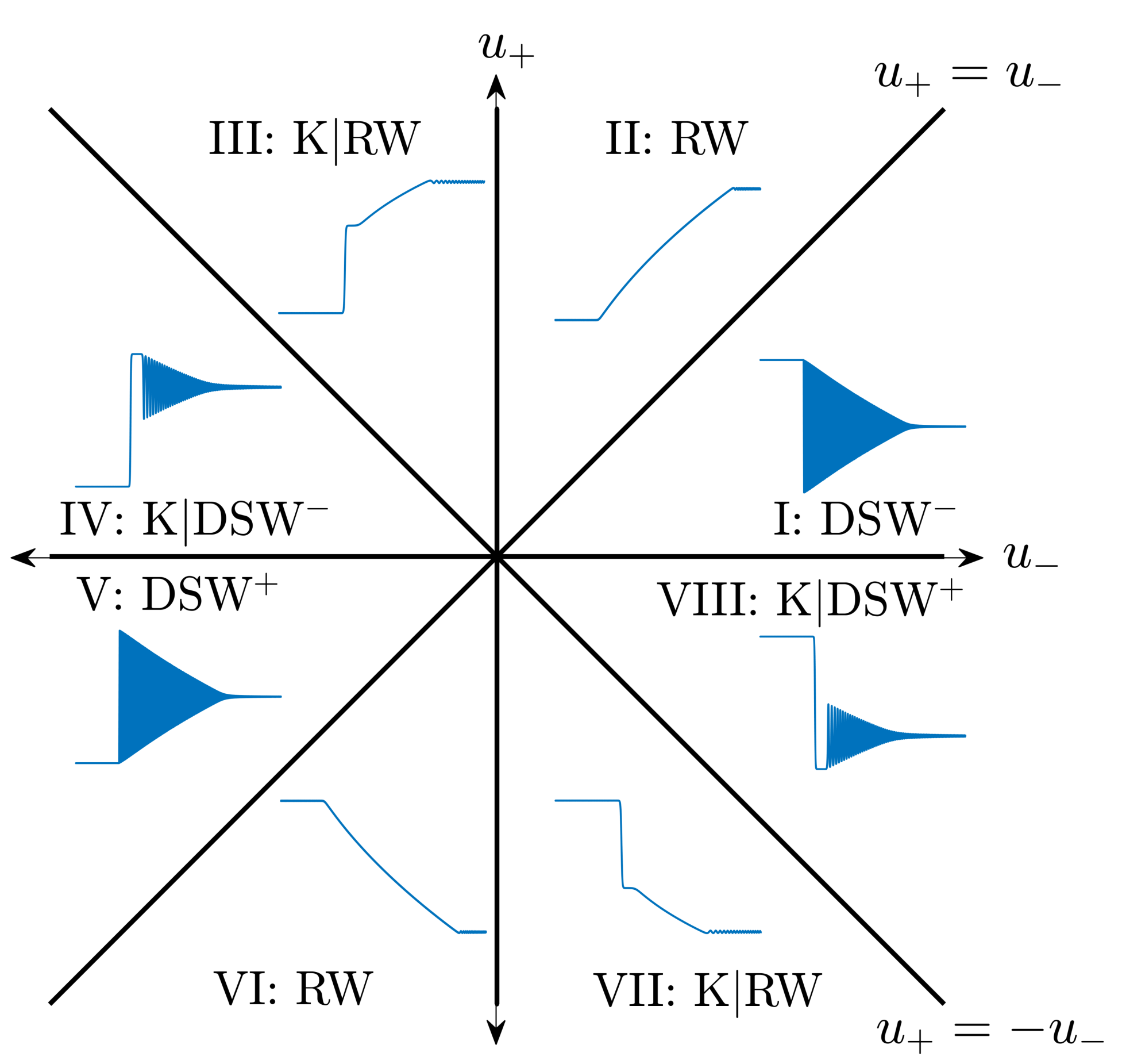
(a) $\mu>0$

(b) $\mu<0$

Figure 4: Classification of the mKdV GP problem in terms of the initial values $u_{\pm}$ with representative numerical solutions, see [37], [14]. Legend: (RW) rarefaction wave, (DSW^+/-) bright/dark dispersive shock wave, (K) kink, (CDSW^+/-) bright/dark contact DSW.

Owing to its universality as a model of weakly nonlinear, long dispersive waves [14], the mKdV equation provides a fundamental description of the GP problem for other PDEs with nonconvex flux.

Rarefaction waves and DSWs solve the GP problem in certain convex and nonconvex cases. Dispersive shock waves are classified as DSW⁺ and DSW^- according to the polarity of the solitary wave generated at one of the edges—leading or trailing, depending on the DSW orientation. In the nonconvex case, we see the emergence of additional wave structures. These occur when the hydrodynamic flux $f(u)=u^{3}$ exhibits an inflection point $u=0$ within the range of step data (4) so that $u_{+}u_{-}<0$. Particularly, when $\mu>0$, and $u_{-}=-u_{+}$, the long-time asymptotic solution is a kink, which is an undercompressive shock in the limit $\mu\to 0^{+}$. When $\mu<0$ and $u_{-}=-u_{+}$, the long-time asymptotic solution is a contact DSW whose leading, algebraic soliton edge is a dispersionless characteristic with velocity $3\bar{u}^{2}$ as $\mu\to 0^{-}$. For other configurations with steps that pass through 0, the solution develops into a hybrid double wave structure as seen in Fig. 4. We stress that in the DSW case, the mean flow is interpreted as the local period average of the DSW’s oscillations.

We now present explicit expressions for the basic mean flows occurring in the mKdV Riemann problem, distinguishing between convex and nonconvex solutions. For brevity, we shall call them convex and nonconvex mean flows, respectively.

5.1 Convex mean flows

RW mean flows (Regions II and VI)

RWs that emerge from the Riemann problems in Regions II and VI of Fig. 4 are described to leading order by

$$\bar{u}(x,t)=\left\{\begin{array}[]{ll}u_{-},&x<3u_{-}^{2}t\\ \text{sgn}(u_{+}-u_{-})\sqrt{\frac{x}{3t}},&3u_{-}^{2}t<x<3u_{+}^{2}t\\ u_{+},&x>3u_{+}^{2}t.\end{array}\right.$$ (72)

This is the long-time approximation of the full mKdV solution that includes dispersive regularisation of weak discontinuities at $x=3u_{\pm}^{2}t$.

DSW mean flows (Regions I and V)

The GP modulation solution describing a DSW depends on the sign of the dispersion coefficient.

According to [14] for $\mu>0$ a DSW⁺ is realized as the solution to the Riemann problem with $u_{-}<u_{+}<0$, see quadrant V in Fig. 4(a). The relevant GP solution to the mKdV modulation equations (54) is a centred simple wave given by

$$\lambda_{1}=u_{-},\quad\lambda_{3}=u_{+},\quad W_{2}(u_{-},\lambda_{2},u_{+})=\frac{x}{t},$$ (73)

where the characteristic speed $W_{2}$ is given by (57), (58) so

$$W_{2}(u_{-},\lambda_{2},u_{+})=u_{-}^{2}+u_{+}^{2}+\lambda_{2}^{2}+2(u_{-}^{2}-\lambda_{2}^{2})\frac{(1-m)K(m)}{E(m)-(1-m)K(m)},\quad m=\frac{\lambda_{2}^{2}-u_{-}^{2}}{u_{+}^{2}-u_{-}^{2}}.$$ (74)

To obtain the mean flow $\bar{u}$ through a DSW, we average the mKdV periodic solution for $u$ over a period. Integrating (38) over the period $2K(m)$ and writing the solution in terms of the Riemann invariants gives

$$\bar{u}=-(\lambda_{1}+\lambda_{2}+\lambda_{3})+2\frac{(\lambda_{2}+\lambda_{3})}{K(m)}\Pi\left(\frac{\lambda_{1}-\lambda_{2}}{\lambda_{1}+\lambda_{3}},m\right),$$ (75)

where $\Pi$ is the complete elliptic integral of the third kind. The dependence $\bar{u}(x,t)$ is obtained by inserting the modulation solution (73), (74) in (75).

For $\mu<0$, a similar averaging over a period of (46) gives

$$\bar{u}=\lambda_{1}+\lambda_{2}-\lambda_{3}-2\frac{(\lambda_{1}+\lambda_{2})}{K(m)}\Pi\left(\frac{\lambda_{2}+\lambda_{3}}{\lambda_{3}-\lambda_{1}},m\right).$$ (76)

For a DSW⁺ with $u_{-}>u_{+}>0$ (quadrant I in Fig. 4(b)), the GP solution to the modulation equations is

$$\lambda_{1}=-u_{-},\quad\lambda_{3}=u_{+},\quad W_{2}(-u_{-},\lambda_{2},u_{+})=\frac{x}{t},$$ (77)

where the characteristic speed is given by (56), (58) is

$$W_{2}=u_{-}^{2}+u_{+}^{2}+\lambda_{2}^{2}+2(u_{+}^{2}-\lambda_{2}^{2})\frac{(1-m)K(m)}{E(m)-(1-m)K(m)}.$$ (78)

Either (74) or (78) gives a parameterisation of the DSW mean flow in terms of $\lambda_{2}\in(u_{-},u_{+})$, yielding $W_{2}(\bar{u})$. This behaviour is not affected by the sign of the dispersion coefficient $\mu$.

For solutions between the roots $u_{1}$ and $u_{2}$, the DSW^- mean flow can be found by applying the transformation (51).

For application to soliton-DSW mean flow interaction, it is instructive to write down the evolution equation for the DSW mean flow $\bar{u}(x,t)$, the simple-wave equation

$$\bar{u}_{t}+W_{2}(\bar{u})\bar{u}_{x}=0.$$ (79)

As a matter of fact, $\bar{u}(x,t)$ given by (75), (73) (or (76), (77)) satisfies equation (79). The advantage of using the PDE (79), instead of the explicitly prescribed mean flow $\bar{u}(x,t)$ will become clear later, in Section 7, where we shall use it instead of the original mean flow equation $\bar{u}_{t}+f^{\prime}(\bar{u})\bar{u}_{x}=0$ as part of the solitonic modulation system (15).

5.2 Nonconvex mean flows

As we have mentioned, nonconvex mean flows are generated if the Riemann data (4) satisfy $u_{-}u_{+}<0$. In contrast to two-parameter convex mean flows, nonconvex mean flows are constrained, one-parameter families of mKdV solutions and, because of this, generally occur in combination with a convex mean flow—either a RW or DSW, see regions III, IV, VII, VIII in Fig. 4. The two classes of “pure” nonconvex mKdV mean flows are kinks described by (45) for $\mu>0$ and contact DSWs (CDSWs) when $\mu<0$ described by modulated trigonometric solutions (49) that exhibit an algebraic soliton (50) at one of its edges.

Kink mean flows ($\mu>0$, $u_{+}=-u_{-}$).

Unlike other mean flows that solve the mKdV GP problem, kinks are localised, steady transitions between antisymmetric means $\bar{u}(-\infty)=u_{-}$ and $\bar{u}(+\infty)=u_{+}=-u_{-}$ described by (45). It has been shown in [47] that kinks dominate the long-time asymptotic solution of defocusing mKdV Riemann problems with antisymmetric data. Kinks are special in the sense that, in addition to considering them as mean flows, we can also treat them as localised soliton solutions that interact with convex mean flows such as RWs and DSWs.

In the limit $\mu\to 0^{+}$, kinks are the weak discontinuous solutions

$$\bar{u}(x,t)=\left\{\begin{array}[]{ll}u_{-},&x<u_{-}^{2}t,\\ -u_{-},&x>u_{-}^{2}t,\end{array}\right.$$ (80)

of the hydrodynamic modulation equation $\bar{u}_{t}+(\bar{u}^{3})_{x}=0$ for the solitonic modulation system. The weak solution (80) represents an undercompressive shock [25, 48] since the hydrodynamic characteristic velocity $c=3u_{-}^{2}=3u_{+}^{2}$ is the same on both sides of the shock.

CDSW mean flows ($\mu<0$, $u_{+}=-u_{-}$)

A CDSW is a modulated trigonometric solution (49) connecting antisymmetric states $u_{-}$ and $-u_{+}$, the negative dispersion counterpart of the kink solution. The CDSW mean flow is given by (76) with $\lambda_{2}=\lambda_{3}$ for CDSW⁺ and $\lambda_{3}=-\lambda_{2}$ for CDSW^-.

For CDSW⁺, realised when $u_{-}>0$, we have

$$\bar{u}=\lambda_{1}+2\sqrt{\lambda_{1}^{2}-\lambda_{3}^{2}},$$ (81)

where the modulations of $\lambda_{1}$ and $\lambda_{3}$ are given by [14]

$$\lambda_{1}=-u_{-},\quad W_{2}=W_{3}=-3u_{-}^{2}+6\lambda_{3}^{2}=\frac{x}{t}.$$ (82)

As earlier, the mean flow variations satisfy equation (79).

Although we call the CDSW mean flow nonconvex because its existence necessitates nonstrict hyperbolicity of the mKdV-Whitham modulation equations, the mean flow characteristic velocity $W_{2}(\bar{u})$ in a CDSW is monotone along the simple wave solution curve (82).

6 mKdV soliton-mean flow interaction: transmission and phase conditions

In order to obtain solutions to the soliton-mean interaction problem, we seek simple wave solutions to the augmented solitonic modulation system (65), (66) in which $q$ and $kp(q,\bar{u})$ are constant while the remaining Riemann invariant, the mean flow $\bar{u}$, varies.

The ordering of the roots $u_{i}$ leads to constraints on the background and amplitudes of the initial solitons. To simplify our analysis, we will consider initial bright solitons in the tunnelling problem. The solution for dark solitons can be obtained using the fact that the mKdV equation is invariant under the transformation (51). For $\mu>0$, the amplitude of an initial bright soliton must satisfy (42): $\bar{u}<0$ and $0<a<-2\bar{u}$. For $\mu<0$, an initial bright soliton must satisfy (48): $\bar{u}\in\mathbb{R}$ and $a>-4\bar{u}$.

For both signs of $\mu$, the transmission and phase conditions can be determined from (28), (29), (64), (71) as

$$\frac{a_{+}}{2}+u_{+}=\frac{a_{-}}{2}+u_{-},\qquad\frac{k_{-}}{k_{+}}=\sqrt{\frac{q_{-}^{2}-u_{-}^{2}}{q_{+}^{2}-u_{+}^{2}}}=\sqrt{\frac{\frac{1}{4}a_{-}^{2}+a_{-}u_{-}}{\frac{1}{4}a_{+}^{2}+a_{+}u_{+}}}.$$ (83)

Notably, these transmission and phase conditions are exactly the same as those for the KdV equation $u_{t}+(u^{2})_{x}=\mu u_{xxx}$ with convex flux [52]. Although, for mKdV, the conditions apply for both positive and negative soliton amplitudes.

A tunnelling condition (33) fails when the characteristic speeds $f^{\prime}(\bar{u})$ and $C(q,\bar{u})$ cross, which occurs when (see (68))

$$q^{2}=\bar{u}^{2}\implies a\in\{0,-4\bar{u}\}.$$ (84)

Crossing through $a=0$ gives the same condition as in the convex case, where for bright solitons, $a>0$ on the transmitted side implies tunnelling, and $a\leq 0$ means the soliton is trapped. For dark solitons, the inequalities must be reversed.

The additional tunnelling condition resulting from nonconvexity when $\bar{u}<0$ is the constraint (48) that the amplitude does not pass through $-4\bar{u}$. When $a\to-4\bar{u}$, we again have trapping, but with a non-zero amplitude and speed $3\bar{u}^{2}$. This limit corresponds to an algebraic soliton. When $\mu>0$, the initial amplitude will be less than $-4u_{\pm}$ since (42) holds for valid bright solitons, and so the transmitted amplitude must also be smaller than $-4u_{\mp}$. For $\mu<0$, initial amplitudes must satisfy (48), so the transmitted amplitude must also be greater than $-4u_{\mp}$.

Considering the intersection of the characteristic speeds is the most direct way to verify the admissibility criteria (33) for the soliton to tunnel through the mean flow. However, we can also see how the phase and transmission conditions (83) are affected. The phase shift $\Delta$ can be obtained from the relation (31), yielding for mKdV

$$\frac{\Delta}{x_{-}}=\sqrt{\frac{\frac{1}{4}a_{-}^{2}+a_{-}u_{-}}{\frac{1}{4}a_{+}^{2}+a_{+}u_{+}}}-1$$ (85)

for the forward (left to right) soliton transmission through a mean flow. If $a_{+}=-2u_{+}$ as when strict hyperbolicity is lost, then from (83) we have $\frac{k_{-}}{k_{+}}\to\infty$. For the backward (right to left) transmission one simply interchanges $``+"$ and $``-"$ in eq. (85).

7 Soliton-convex mean flow interaction

First, we consider the tunnelling problem in the classical case of convex mean flows: rarefaction waves (RWs) and dispersive shock waves (DSWs). However, nonconvexity of the mKdV equation makes the problem novel in the sense that both bright and dark solitons exist. We see that the additional admissibility criterion of strict hyperbolicity leads to more restrictive tunnelling conditions than in the convex case. When trapping occurs in situations with soliton amplitudes $a>0$, we find that an exponentially decaying soliton limits to an algebraic soliton when $a\to-4\bar{u}>0$.

7.1 Soliton tunnelling through RWs: Regions II and VI

Rarefaction waves that emerge from the GP problems in Regions II and VI of Fig. 4 are described to leading order by eq. (72). The RW is confined to the interval $3u_{-}^{2}t<x<3u_{+}^{2}t$.

To determine the admissible directionality for soliton-mean interaction, an admissible soliton’s velocity must be compared to the edge velocity of the RW. For $\mu>0$, it is only possible for solitons to travel from right to left, implying backward soliton-mean interaction while for $\mu<0$, solitons can only go from left to right. Soliton tunnelling occurs in either case if the system maintains strict hyperbolicity and $a\neq 0$. The tunnelling parameters are determined by the transmission conditions (83).

For $\mu>0$, we focus on RWs in region VI of Fig. 4 because bright solitons are admissible. The case of region II with dark soliton-RW interaction can be obtained by the transformation (51). Initialising $x_{0}=x_{+}$, $u_{+}<0$, $0<a(x_{+},0)=a_{+}<-2u_{+}$, we only need to check that $0<a_{-}<-4u_{-}$ for $u_{+}<u_{-}<0$ to prove that the characteristic speeds did not cross because the RW transitions continuously and monotonically from $u_{-}$ to $u_{+}$. We use the transmission condition (83) to express this inequality in terms of the initial soliton amplitude $a_{+}$ for a bright soliton starting on the right,

$$2(u_{-}-u_{+})<a_{+}<-2(u_{+}+u_{-}).$$ (86)

The second inequality is automatically satisfied by any valid initial soliton. Hence, the first is a sufficient condition for tunnelling,

$$a_{+}>a_{cr}=2(u_{-}-u_{+}).$$ (87)

Since $u_{+}<u_{-}<0$ in region VI, (87) gives a positive critical amplitude for transmission to occur. A numerical example of a soliton tunnelling through a RW in this case is shown in Fig. 5.

Figure 5: Soliton-RW interaction with $\mu=1$, $a_{+}=1.5$, $x_{+}=100$, $u_{-}=-1$, $u_{+}=-1.5$. The amplitude $a_{-}$ predicted by the transmission condition (83) is 0.5, and the predicted phase shift $\Delta$ is 96.40. The numerical solution gives $a_{-}=0.4981$ and $\Delta=95.02$ at $t=300$.

The soliton trajectory is specified by $\mathrm{d}x/\mathrm{d}t=C(q,\bar{u})$, where $C(q,\bar{u})$ is given by (70). Integrating this equation we obtain

$$x(t)=\left\{\begin{array}[]{ll}(u_{-}^{2}+2q^{2})t+E,&x<3u_{-}^{2}t\\ 3q^{2}t+Dt^{1/3},&3u_{-}^{2}t<x<3u_{+}^{2}t\\ (u_{+}^{2}+2q^{2})t+x_{+},&x>3u_{+}^{2}t\end{array}\right.$$ (88)

where $D$ and $E$ are obtained by continuity of $x(t)$

$$D =\frac{3}{2}x_{+}^{2/3}(2u_{+}^{2}-2q^{2})^{1/3}$$ (89)

$$E =x_{+}\sqrt{\frac{u_{+}^{2}-q^{2}}{u_{-}^{2}-q^{2}}}.$$ (90)

The phase shift is $\Delta=E-x_{+}$, which matches the condition given by (83).

A similar analysis can be carried out for each region in Fig. 4 to determine the tunnelling criterion. We summarise the remaining results without detailing the analysis for each case in Table 1 for either sign of $\mu$ in Regions II and VI. Note that for $\mu<0$ in Region VI, the tunnelling criterion is different than the condition that $a_{+}>0$. This is because there are cases for valid initial soliton amplitudes $a_{-}$ where the amplitude crosses $-4\bar{u}$ during interaction with the RW, causing the soliton to become trapped and travel too slowly to reach the other side. In the limit as $t\to\infty$, the trapped soliton becomes an algebraic soliton travelling at constant hydrodynamic characteristic velocity $3\bar{u}^{2}$.

Figure 6 illustrates the loss of strict hyperbolicity when $\mu<0$ for nonzero amplitudes by depicting the wave curves $a(\bar{u})$ corresponding to constant $q(a,\bar{u})$ and the corresponding soliton speed $c(a(\bar{u}),\bar{u})$. For interaction to occur in region VI, solitons are initialised on the left at $x_{0}=x_{-}$ with mean flow $u_{-}<0$ (we take $u_{-}=-1$ for definiteness) and amplitudes satisfying (42). For initial amplitudes $-4u_{-}<a_{-}<a_{cr}=-2(u_{+}+u_{-})$, solitons pass through the mean flow from $u_{-}$ to $u_{+}<u_{-}$ ($u_{+}=-2$ for definiteness) maintaining positive amplitude. But these wave curves eventually intersects the critical line $-4\bar{u}$ (shown in red). In Fig. 8(b), the corresponding soliton speeds are plotted. Intersection of $a(\bar{u})$ with $-4\bar{u}$ corresponds to the intersection of the soliton velocity $c(a,\bar{u})$ with the characteristic velocity $3\bar{u}^{2}$, also shown in red. As the two coincide, the soliton asymptotically limits to a trapped algebraic soliton propagating with characteristic velocity.

Dispersion	Direction	Region II - RW ($u_{+}>u_{-}>0$)	Region VI - RW ($u_{+}<u_{-}<0$)
$\mu>0$	$R\to L$	No bright soliton solutions	Tunnelling if $a_{+}>a_{cr}=2(u_{-}-u_{+})$
$\mu<0$	$L\to R$	Tunnelling if $a_{-}>a_{cr}=2(u_{+}-u_{-})$	Tunnelling if $a_{-}>a_{cr}=-2(u_{+}+u_{-})$

Table 1: Results for the bright soliton tunnelling problem through RWs. $R\to L$ means that $x_{0}=x_{+}$ and the soliton propagates from right ($R$) to left ($L$), otherwise $x_{0}=x_{-}$ ($L\to R$).

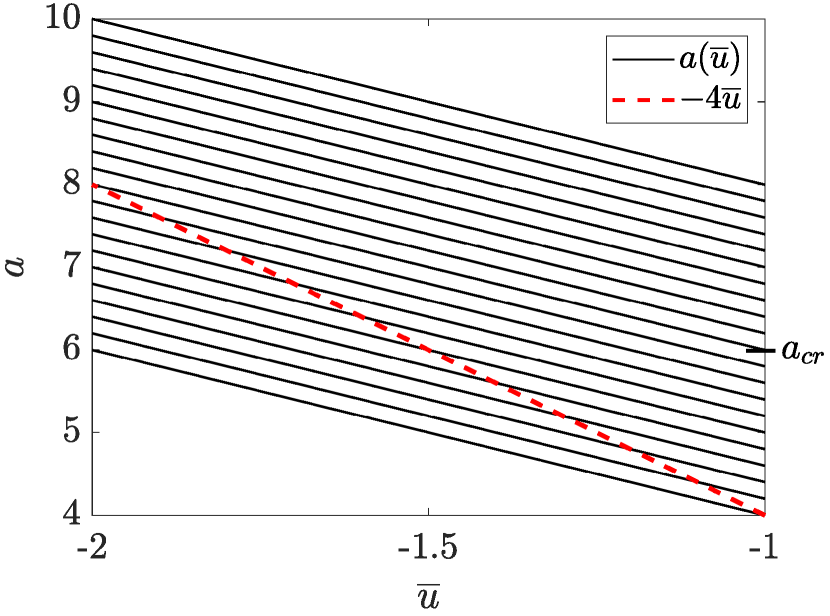
(a) Soliton amplitudes.

(b) Soliton velocities.

Figure 6: Simple wave curves of constant $q(a,\bar{u})$ (solid) and curves of nonstrict hyperbolicity (dashed) illustrating interaction with a RW with $u_{-}=-1$, $u_{+}=-2$ and $\mu=-1$ for various initial amplitudes $a_{-}$. Left: soliton amplitudes as a function of $\bar{u}$; right: soliton speeds. When travelling from $u_{-}$ to $u_{+}$ with $a_{-}<a_{cr}$, the solid and dashed curves intersect, corresponding to loss of strict hyperbolicity.

7.2 Soliton tunnelling through DSWs: Regions I and V

For $\mu>0$, the DSW leading and trailing edge velocities for both regions I and V of Fig. 4 are given by $s_{+}=6u_{-}^{2}-3u_{+}^{2}$ and $s_{-}=u_{-}^{2}+2u_{+}^{2}$ [14]. Comparing the soliton’s initial velocity to the edge velocities, we see that there can be interaction in both directions in region V ($u_{-}<u_{+}<0$). In region I ($0<u_{+}<u_{-}$), bright soliton solutions do not exist.

First, we consider the backward interaction in region V in which $x_{0}=x_{+}$. For the interaction to occur, the soliton speed $c(a_{+},u_{+})$ must be smaller than $s_{+}$, which gives the condition

$$2(u_{-}-u_{+})<a_{+}<-2u_{+}.$$ (91)

This condition is satisfied for any admissible, initial bright soliton $a_{+}$. It and the transmission condition (83) imply that $0<a_{-}<-4u_{-}$ so, invoking monotonicity of the DSW mean flow, we can see that strict hyperbolicity and amplitude positivity is maintained along the soliton trajectory. The soliton will always tunnel.

Next, we consider forward interaction where $x_{0}=x_{-}$. In order for the soliton to overtake the DSW, we require $c(a_{-},u_{-})>s_{-}$, which implies that

$$q^{2}>u_{+}^{2}.$$ (92)

Then one of

$$a_{-}>-2(u_{+}+u_{-}),\quad\text{ or }\quad a_{-}<2(u_{+}-u_{-})$$ (93)

holds. The first inequality in (93) cannot be satisfied for an admissible, initial bright soliton constrained by (42). The second inequality in (93) can be satisfied by an initial bright soliton, but (83) implies that $a_{+}<0$ so the soliton is trapped. We can also see this by comparing the characteristic velocities $c(a_{-},u_{-})$ and $3u_{-}^{2}$ where valid initial soliton amplitudes $a_{-}$ satisfying (42) result in $q^{2}<u_{-}^{2}$. Since $q^{2}>u_{+}^{2}$ is necessary for the interaction to occur (see (92)), $u_{+}^{2}>u_{-}^{2}$, and $\bar{u}$ is continuous, the velocities must intersect and therefore the soliton is trapped by the DSW.

For $\mu<0$, the DSW leading and trailing edge speeds are given by $s_{+}=u_{+}^{2}+2u_{-}^{2}$ and $s_{-}=6u_{+}^{2}-3u_{-}^{2}$ [14]. Initial solitons with either $x_{0}=x_{+}$ or $x_{0}=x_{-}$ can exist in both Regions I and V and the tunnelling criterion can again be determined by comparing velocities and then looking at the admissibility criterion for tunnelling. Table 2 summarises the results for bright soliton-DSW interaction.

Dispersion	Direction	Region I - DSW ($u_{-}>u_{+}>0$)	Region V - DSW ($u_{-}<u_{+}<0$)
$\mu>0$	$R\to L$	No soliton solutions	Tunnelling always occurs
	$L\to R$	No soliton solutions	Interaction and trapping if $a_{-}<2(u_{+}-u_{-})$
$\mu<0$	$R\to L$	No interaction	Interaction and trapping if $a_{+}<-2(u_{+}+u_{-})$
	$L\to R$	Tunnelling always occurs	Tunnelling if $a_{-}>a_{cr}=2(u_{+}-u_{-})$

Table 2: Results for the bright soliton-DSW interaction problem.

Numerical experiments on soliton tunnelling through DSWs were conducted for both signs of $\mu$ with results given in Table 3 and Table 4. Good agreement was found between the predicted amplitude and phase shift (equations (83), (85)) and the numerical results, confirming that hydrodynamic reciprocity is maintained. Figure 7 shows one sample numerical solution.

$u_{+}$	$u_{-}$	$a_{+}$	$T_{final}$	$a_{-}$ (pred)	$a_{-}$ (num)	$\Delta x/x_{-}$ (pred)	$\Delta x/x_{-}$ (num)
-1	-1.5	0.1	300	1.1	1.0968	-0.7310	-0.7226
-1	-1.5	0.5	200	1.5	1.4914	-0.4908	-0.4880
-1	-1.5	1	100	2	1.9960	-0.3876	-0.3833

Table 3: Numerical tests of backward ($R\to L$) bright soliton-DSW interaction for $\mu=1$ and $x_{+}=100$ in Region V.

$u_{-}$	$u_{+}$	$a_{-}$	$T_{final}$	$a_{+}$ (pred)	$a_{+}$ (num)	$\Delta x/x_{-}$ (pred)	$\Delta x/x_{-}$ (num)
1.5	1	0.1	170	1.1	1.0989	-0.6703	-0.6577
1.5	1	0.5	170	1.5	1.4740	-0.3724	-0.3590
1.5	1	1	70	2	1.9818	-0.2362	-0.2320
-0.6	-0.1	2.6	100	1.6	1.5966	-0.4796	-0.4539

Table 4: Numerical tests of forward ($L\to R$) bright soliton-DSW interaction, $\mu=-1$ and $x_{-}=100$ in Region I and V.

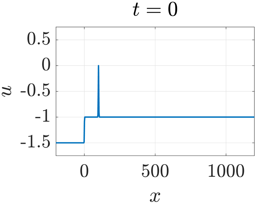
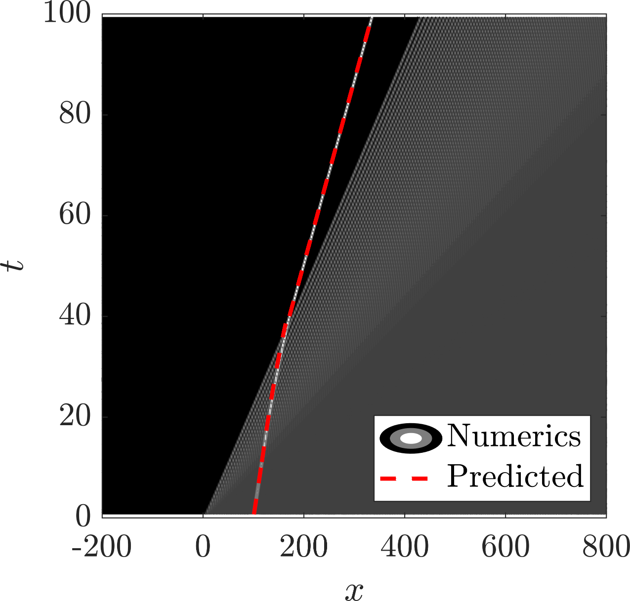
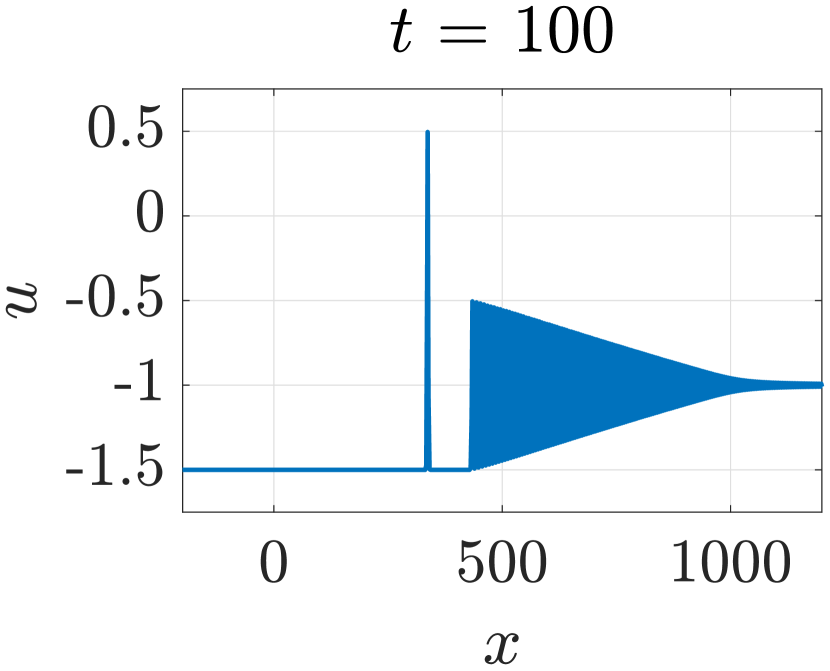
Figure 7: Soliton-DSW interaction with $\mu=1$, $a_{+}=1$, $x_{+}=100$, $u_{-}=-1.5$, and $u_{+}=-1$. The predicted $a_{-}$ is 2 and the predicted $\Delta$ is $-38.76$. At $t=100$, the numerical solution gives $a_{-}=1.9960$ and $\Delta=-38.33$.

For a RW, the soliton trajectory $x(t)$ and amplitude $a(\bar{u})$ throughout the soliton-RW interaction is known. In contrast, the mean flow $\bar{u}(x,t)$ for a DSW is given by the modulation of a periodic travelling wave and is more complicated. Although the soliton amplitude and phase shift on either side of the DSW can be predicted without knowing the space-time variation of the mean flow in the DSW’s interior by invoking hydrodynamic reciprocity (see Section 3.3), the Riemann invariants $q$ and $kp$ of the augmented solitonic system (65), (66) are not held constant throughout the DSW. What is desired is some way to estimate the wave curve $a(\bar{u})$ within the DSW. Since $\bar{u}$ is known and now described by equation (79) rather than $\bar{u}_{t}+f^{\prime}(\bar{u})\bar{u}_{x}=0$, we require an alternative approach to approximating the wave curve $a(\bar{u})$.

To obtain $a(\bar{u})$ along the soliton trajectory $\mathrm{d}x/\mathrm{d}t=c(a,\bar{u})$, we make an assumption that soliton-DSW interaction can be approximated by the interaction of a soliton with the DSW mean flow, and take advantage of the characteristic ODE (17) in which we replace the characteristic velocity $f^{\prime}(\bar{u})$ in the RW solution with the characteristic velocity $W_{2}(\bar{u})$ of the simple wave equation (79) for the DSW modulation solution. The velocity $W_{2}(\bar{u})$ is specified parametrically by (74), (75) (or equivalently, (78), (76)). Thus, we obtain the ODE

$$\frac{\mathrm{d}\tilde{k}}{\mathrm{d}\bar{u}}=\frac{\partial_{\bar{u}}\tilde{\omega}_{0}}{W_{2}(\bar{u})-\partial_{\tilde{k}}\tilde{\omega}_{0}},\quad\tilde{k}(u_{-})=\tilde{k}_{-},$$ (94)

where, as earlier, $\tilde{\omega}_{0}=-i\omega_{0}(i\tilde{k},\bar{u})$ and $\omega_{0}(k,\bar{u})$ is the mKdV linear dispersion relation (35). The relation between the conjugate wavenumber $\tilde{k}$ and the soliton amplitude $a$ is given by equation (18), which is

$$\tilde{k}^{2}=-\frac{1}{\mu}\left(\frac{1}{2}a^{2}+2a\bar{u}\right),$$ (95)

so that $\tilde{k}_{-}$ is (95) evaluated at $a=a_{-}$, $\bar{u}=u_{-}$. Substituting the expression for $W_{2}(\bar{u})$ given by (74) or (78) and the dispersion relation (35) into (94), we can numerically integrate for $\tilde{k}(\bar{u})$ and invert (95) to solve for the approximate wave curve $a(\bar{u})$. Since (95) is double valued, we use the existence conditions (42) for $\mu>0$ and (48) for $\mu<0$ in order to determine the correct value for $a$.

We now consider the implications of this mean flow approach toward understanding soliton-DSW interaction for each sign of $\mu$ separately.

First, for $\mu>0$ and a backward soliton ($x_{0}=x_{+}>0$) tunnelling through a DSW⁺ (region V), Fig. 8(a) shows the wave curves $a(\bar{u})$ representing the soliton amplitude as it passes through the DSW mean flow with corresponding local trajectory velocity in Fig. 8(b). As expected from Table 2, the soliton always tunnels through the DSW from right to left ($x_{0}=x_{+}>0$). For any valid initial positive amplitude satisfying $0<a_{+}<-2u_{+}$ (42), the soliton’s amplitude neither crosses the critical line $-2\bar{u}$ nor decays to zero during propagation. Correspondingly, the velocities of solitons starting at $u_{+}=-1$ and moving to $u_{-}=-1.5$ mostly remain below the DSW velocity $W_{2}(\bar{u})$, save for very small $a_{+}$. However, examining solitons travelling from left to right ($x_{0}=x_{-}<0$), if the initial amplitude is below the critical value $a_{-}<a_{cr}=2(u_{+}-u_{-})$, the soliton is trapped and the amplitude decays to zero. The initial amplitudes below $a_{cr}$ in Fig. 8(a) correspond to the velocities in Fig. 8(b) that lie between $3\bar{u}^{2}$ and the characteristic $W_{2}(\bar{u})$, indicating that the soliton is trapped. Initial amplitudes satisfying $a_{-}>a_{cr}$ correspond to soliton velocities that never catch up to the DSW, $c(a_{-},u_{-})<W_{2}(u_{-})$, so soliton-DSW interaction doesn’t occur.

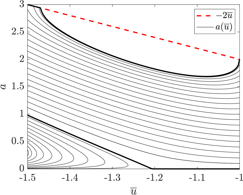
(a) Soliton amplitudes.

(b) Soliton velocities.

Figure 8: Wave curves (a) and corresponding local velocities (b) of a soliton interacting with a DSW⁺ for $u_{-}=-1.5$, $u_{+}=-1$ and $\mu=1$. When traversing curves from $u_{+}$ to $u_{-}$ with $a_{+}<a_{cr}=$, the curves intersect the characteristics corresponding to loss of strict hyperbolicity. In this case, these amplitudes decay to zero.

We make two consistency checks in Fig. 9. The soliton amplitude $a(u_{-})$ computed from the wave curve $a(\bar{u})$ that includes the point $a(u_{+})=a_{+}$ remains within 8% of $a_{-}=a_{+}+2(u_{+}-u_{-})$ predicted by the transmission condition (83) when $u_{-}=-1.5$, $u_{+}=-1$. This result holds for all initial amplitudes satisfying $0<a_{+}\lessapprox 1.7134$. The upper bound on admissible initial amplitudes is below the critical value $a_{cr}=2$. When $1.7134<a_{+}<2$, the wave curve terminates at $a(\bar{u})=-2\bar{u}$ for $\bar{u}>u_{-}=-1.5$ as shown in Fig. 8(a). The error is shown in Fig. 9 as a function of initial soliton amplitude.

Another consistency check is the predicted phase shift

$$\overline{\Delta}\equiv x_{+}-\Big{(}x(t_{-})-c\big{(}a(u_{-}),u_{-}\big{)}t_{-}\Big{)},\quad\frac{\mathrm{d}x}{\mathrm{d}t}=\frac{\tilde{\omega}(\tilde{k}(x,t),\bar{u}(x,t))}{\tilde{k}(x,t)},\quad x(t_{+})=s_{+}t_{+},$$ (96)

where $t_{\pm}$ are the times that the soliton’s trajectory crosses the DSW’s leading ($s_{+}t$) and trailing ($s_{-}t$) edges. This is compared with the phase shift $\Delta$ determined by the transmission condition (85) in Fig. 9.

Figure 9: Relative error in the predicted transmitted soliton amplitude $a(u_{-})$ and soliton phase shift $\overline{\Delta}$ for soliton-DSW⁺ interaction using the mean flow description from right to left. Parameter values are $\mu=1$, $x_{0}=x_{+}=100$, $u_{-}=-1.5$, and $u_{+}=-1$.

An interesting case where convexity is lost, but the trapped soliton amplitude does not decay to zero is for $\mu<0$ and a soliton interacting with a DSW^- (Region V). Figure 10(a) shows the soliton amplitude as it passes through the DSW and Fig. 10(b) shows the corresponding soliton velocity. When travelling from left to right ($x_{0}=x_{-}<0$) with $u_{-}=-1.5$, admissible solitons satisfying (48) always have velocities faster than $W_{2}(\bar{u})$, so interaction occurs but the velocities never cross $W_{2}(\bar{u})$ so strict hyperbolicity is maintained. This can also be seen in the smooth amplitude curves from $u_{-}$ to $u_{+}$, which never intersect $-4\bar{u}$. However, when the soliton is slow enough to interact from right to left through the DSW from $u_{+}=-1$ to $u_{-}=-1.5$, then the soliton becomes trapped and the velocities lie between $3\bar{u}^{2}$ and $W_{2}(\bar{u})$. This corresponds to amplitudes below the critical amplitude $a_{cr}=2(u_{+}-u_{-})$. For a soliton with amplitudes below this critical amplitude, the velocity crosses $W_{2}$ and limits to $3\bar{u}^{2}$, while the amplitude limits to $-4\bar{u}$, indicating that it behaves like an algebraic soliton.

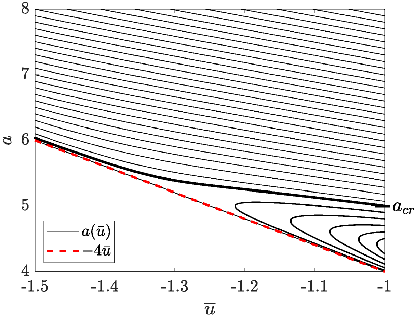
(a) Soliton amplitudes.

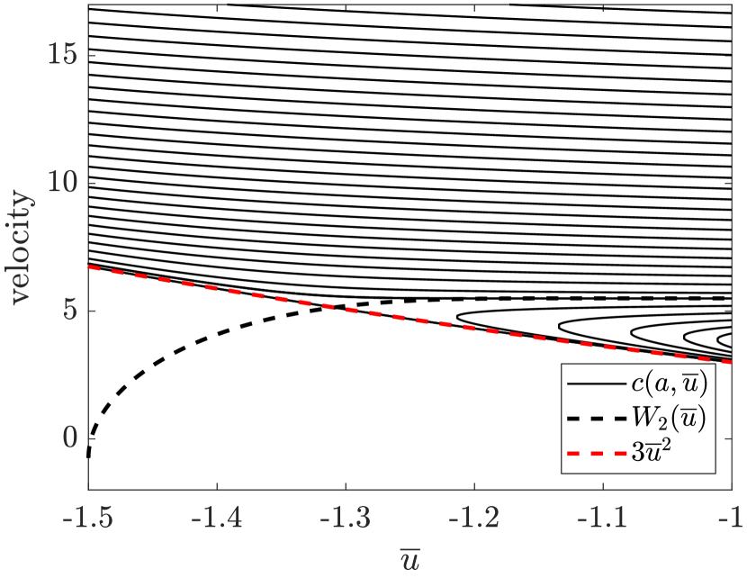
(b) Soliton velocities.

Figure 10: Soliton interaction with a DSW^- with $u_{-}=-1.5$, $u_{+}=-1$ and $\mu=-1$ for various amplitudes. When initialised on the right at $u_{+}$ with $a_{+}<a_{cr}$, the wave curves do not reach $u_{-}$ so the soliton is trapped.

When tunnelling occurs, the transmitted amplitude from numerical integration of the ODE (94) is compared to the amplitude predicted by transmission conditions and the error is shown in Fig. 11. For initial amplitudes that satisfy $a_{-}>6.1$ with $a_{cr}=6$ for $u_{-}=-1.5$ and $u_{+}=-1$, the computed soliton amplitude $a(u_{+})$ is within 1% of the predicted amplitude. The predicted phase shift based on (96) with subscripts $-$ replaced with $+$ is also compared to the phase shift as determined from the transmission condition (85) in Fig 11.

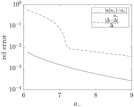
Figure 11: Relative error in the predicted transmitted soliton amplitude $a(u_{+})$ and soliton phase shift $\overline{\Delta}$ for soliton-DSW⁺ interaction using the mean flow description from left to right. Parameter values are $\mu=-1$, $x_{0}=x_{-}=-100$, $u_{-}=-1.5$, and $u_{+}=-1$.

8 Soliton-nonconvex mean flow interaction

In this section, we study interactions of solitons with nonconvex mean flows arising from the mKdV GP problem with $u_{-}u_{+}<0$. We consider interactions with “pure” nonconvex mean flows generated for the symmetric conditions $u_{-}=-u_{+}$. These are kinks ($\mu>0$) and CDSWs ($\mu<0$); see Section 5.2.

8.1 Soliton-kink interaction

A kink solution to the GP problem when $\mu>0$ is realised when $u_{+}=-u_{-}$. To be definite, we assume that $u_{-}<0$. The kink velocity $u_{-}^{2}=u_{+}^{2}$ is slower than the soliton velocity for any amplitude so interaction happens from left to right with $x_{0}=x_{-}<0$. By the soliton existence conditions (42), when $u_{-}<0$, we must initialise with a bright soliton $(a_{-}>0)$ on the left side. Since bright solitons cannot exist on the right side of the kink where $u_{+}>0$, we expect that the soliton polarity undergoes a switch as a result of kink interaction in order for the soliton to be a valid solution. To determine the transmitted soliton amplitude, we observe that, under the quadratic transformation (58), the mKdV soliton-kink interaction problem in the limit $\mu\to 0$ is mapped onto the problem of KdV soliton train propagation on a background $-3\bar{u}^{2}$ described by the modulation system (cf. (62))

$$\frac{\partial r_{1}}{\partial t}-r_{1}\frac{\partial r_{1}}{\partial x}=0,$$ (97)

$$\frac{\partial r_{3}}{\partial t}-\frac{1}{3}(r_{1}+2r_{3})\frac{r_{3}}{\partial x}=0,$$

where $r_{1}=-3\lambda_{1}^{2}$ and $r_{3}=-3\lambda_{3}^{2}$. Since $\lambda_{1}=\bar{u}$, the above quadratic transformation maps the discontinuous solution (80) for $\bar{u}$ to the constant solution $r_{1}=-3\bar{u}^{2}=-3u_{-}^{2}$ of the first equation in (97). The second equation also admits the constant solution $r_{3}=const$, which is mapped to $\lambda_{3}=const$, and therefore $|a|=2(\lambda_{3}-\lambda_{1})=const$ for the mKdV equation.

The transformation of the soliton amplitude in soliton-kink tunnelling can be obtained from the transmission condition (83) by assuming that the normalisation (19) of the Riemann invariant $q=Q(a,\bar{u})$ changes to $Q(0,\bar{u})=-\bar{u}$ when crossing the zero convexity point $\bar{u}=0$ at $x=0$, yielding the transmission condition $u_{+}+\frac{1}{2}a_{+}=-(u_{-}+\frac{1}{2}a_{-})$. Since $u_{-}=-u_{+}$, we obtain $a_{+}=-a_{-}$. Inserting this result into the soliton phase shift formula (85), we obtain $\Delta=0$. To be clear, the predicted zero phase shift is an approximate result within the context of modulation theory in the limit $\mu\to 0$. For nonzero but small $\mu$, a small phase shift due to soliton-kink interaction is expected. Such an interaction for the mKdV equation can be investigated using the inverse scattering transform (IST) with non-zero boundary conditions developed for both signs of $\mu$ in [66]. Within the IST formalism, the conservation of the absolute value of the soliton amplitude pre and post interaction is a consequence of the discrete spectrum’s conservation.

Numerical experiments with results in Table 5 confirm that, as the soliton propagates through the kink, it switches polarity while preserving the absolute value of the amplitude and that the phase shift is very small, as seen in Fig. 12. The observed small phase shift from numerical experiments is due to the nonzero value of $\mu$ used in numerical simulations. Note that the kink itself undergoes a phase shift in the direction opposite to the soliton.

$u_{-}$	$u_{+}$	$a_{-}$	$t_{final}$	$a_{+}$	$a_{+}$ (num)	$\Delta x$	$\Delta x$ (num)	$\Delta x/|x_{-}|$ (num)	$\Delta x_{kink}$
-1	1	0.5	200	-0.5	-0.4991	0	1.6530	0.0331	-2.3438
-1	1	1.0	200	-1.0	-1.0000	0	2.1484	0.0430	-3.8086
-1	1	1.5	500	-1.5	-1.4999	0	3.0273	0.0605	-5.8594
-2	2	1.5	50	-1.5	-1.4988	0	0.9766	0.0195	-1.6113

Table 5: Numerical tests of bright soliton-kink interaction from left to right for $\mu=1$ with $x_{-}=50$. Values for $a_{+}$ and $\Delta x$ according to the transmission conditions are compared with numerical (num) results.

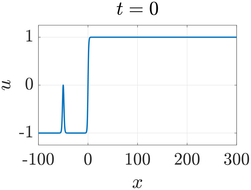
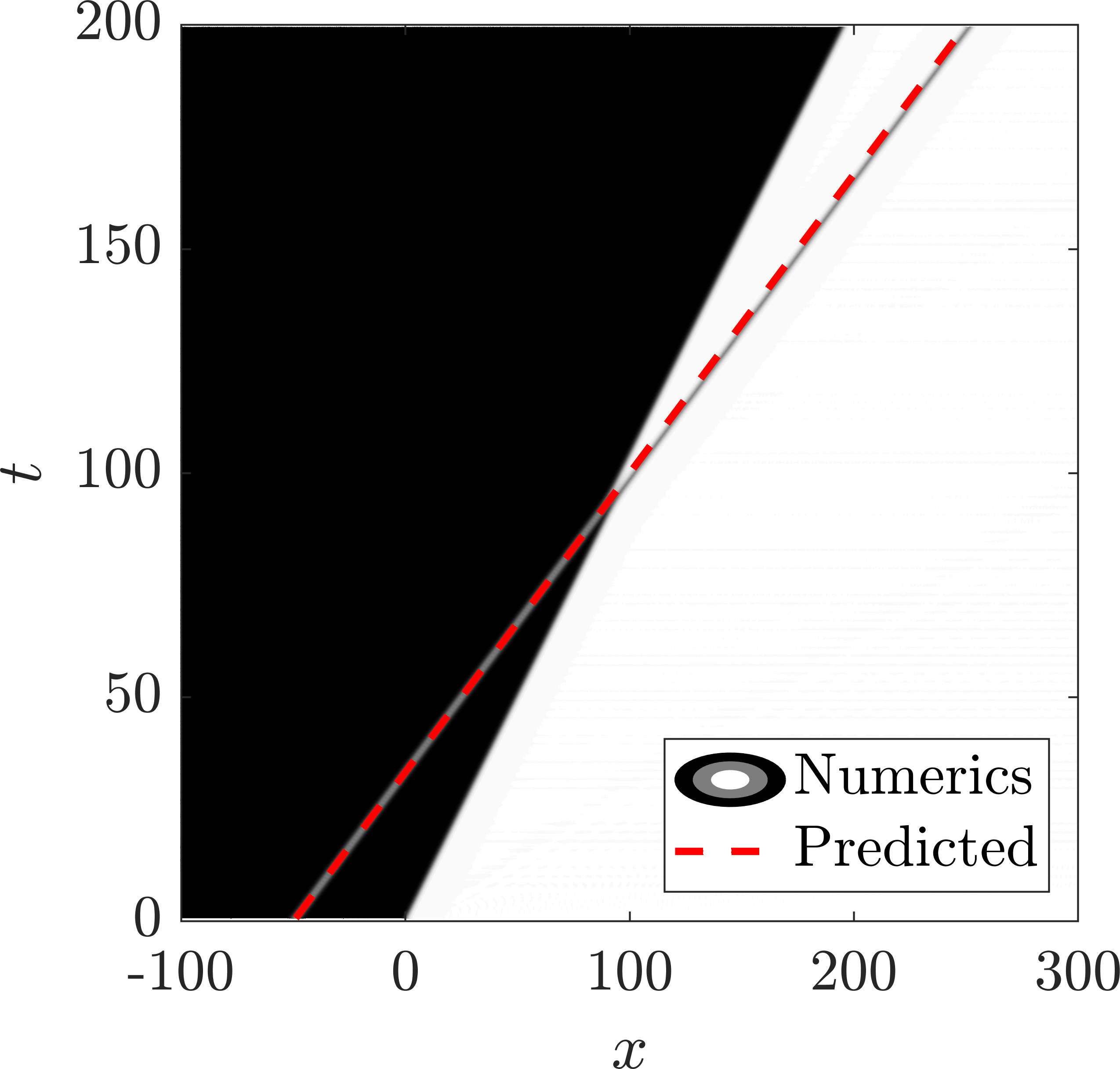
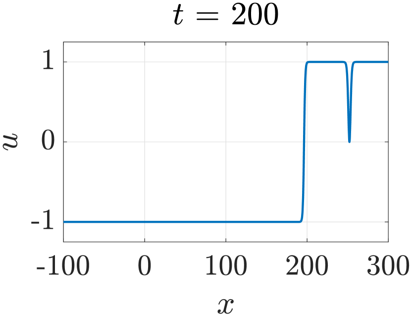
Figure 12: Soliton-kink interaction for $\mu=1$, $a_{-}=1$, $x_{-}=-50$, $u_{-}=-1$, and $u_{+}=1$. The predicted $a_{+}$ is -1, after flipping polarity in the interaction, and the predicted phase shift $\Delta$ is 0. The numerical solution gives $a_{+}=-1.0000$ and $\Delta=2.1484$ at $t=200$.

8.2 Soliton-CDSW interaction

When $\mu<0$ and $u_{-}=-u_{+}$, the resulting solution that emerges from the GP problem is a CDSW. The leading and trailing edge travel at characteristic velocity $s_{+}=3u_{-}^{2}$ and $s_{-}=-3u_{-}^{2}$, so that solitons can only interact with the CDSW from left to right, $x_{0}=x_{-}<0$. Tunnelling always occurs in this interaction and the transmitted amplitude is obtained from (83) as

$$a_{+}=a_{-}+4u_{-}.$$ (98)

By the existence conditions (48), an initial soliton satisfies $a_{-}>-4u_{-}$. To maintain strict hyperbolicity, $a_{+}>-4u_{+}$ as well. Note that the CDSW mean flow is monotone along the characteristic $\mathrm{d}x/\mathrm{d}t=W_{2}(\bar{u})$; see (82). Using the transmission condition, we can see that

$$a_{+} >-4u_{+}$$ (99)

$$\implies a_{-} >2u_{+}-2u_{-}=-4u_{-},$$ (100)

and this relation is always satisfied by $a_{-}$ so strict hyperbolicity is maintained.

The predicted phase shift is found from equation (85) with $u_{+}=-u_{-}$ and $a_{+}$ given by (98). As with the pure kink interaction, $\Delta=0$. Numerical experiments verify the conservation of $q$ and $kp$, although we do see a small phase shift, likely due to higher order effects. See Fig. 13 for depictions of soliton interaction with CDSWs of both polarities at the boundaries of regions VII and VIII (positive polarity) and III and IV (negative polarity). The predicted soliton trajectory (dashed) in Fig. 13 was generated by assuming that it was unchanged by the mean flow, rather than considering the CDSW mean flow given by (81) and the ODE (94). This approximation is justified by the predicted zero phase shift and unchanged soliton velocity post CDSW interaction.

In contrast to the soliton-kink interaction, the soliton-CDSW interaction does not result in the soliton’s polarity change. This is because strict hyperbolicity is maintained throughout and the existence condition (48) for solitons with $\mu<0$ allow for bright solitons on either side of the mean flow.

$u_{-}$	$u_{+}$	$a_{-}$	$T_{final}$	$a_{+}$ (pred)	$a_{+}$ (num)	$\Delta x$ (pred)	$\Delta x$ (num)	$\Delta x/|x_{-}|$ (num)
-0.5	0.5	2.5	120	0.5	0.4993	0	-1.0352	0.0207
0.5	-0.5	1.0	120	3.0	2.9960	0	-0.4688	0.0094

Table 6: Numerical tests of bright soliton-CDSW interaction from left to right for $\mu=-1$ and $x_{-}=-50$.

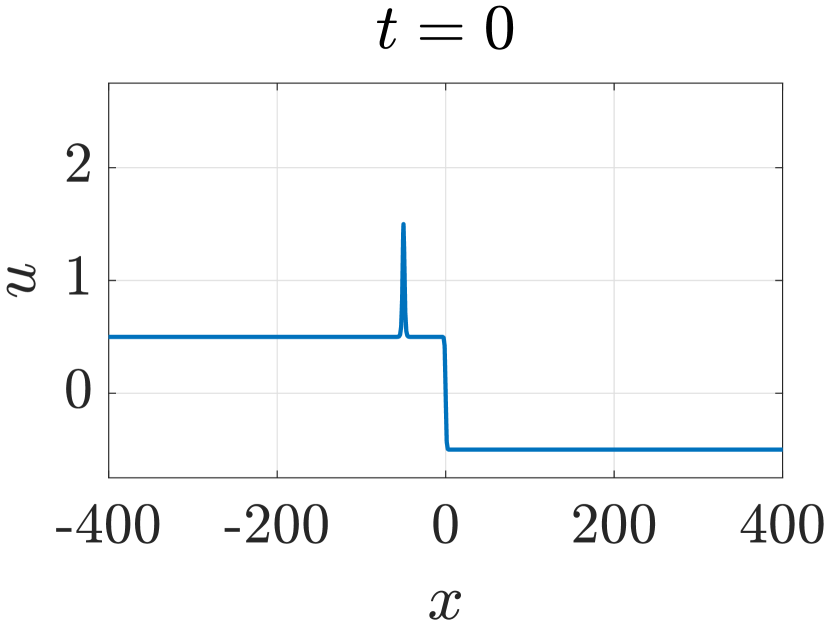
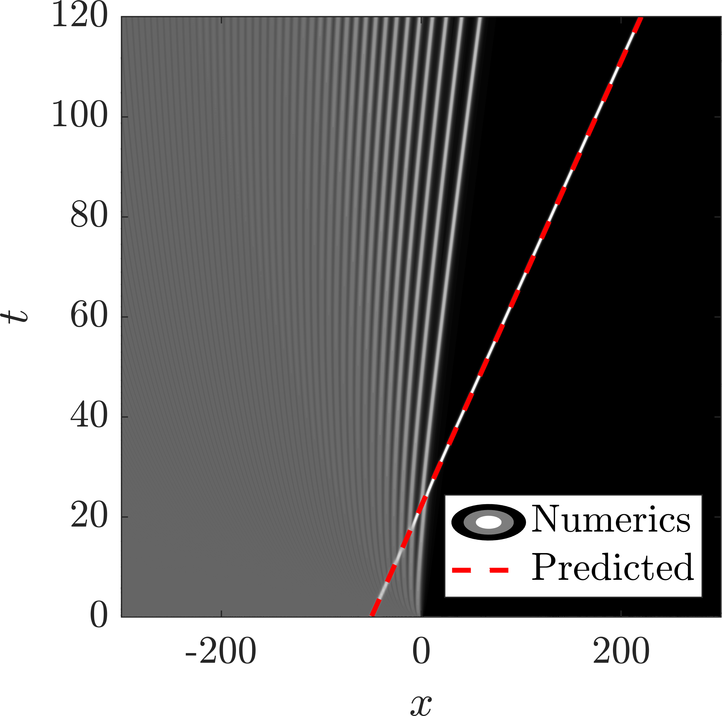
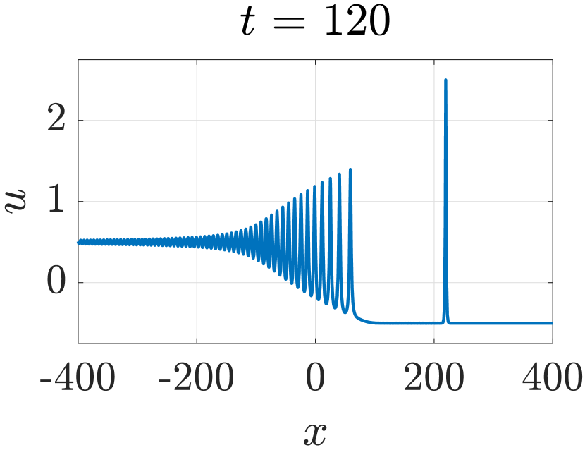
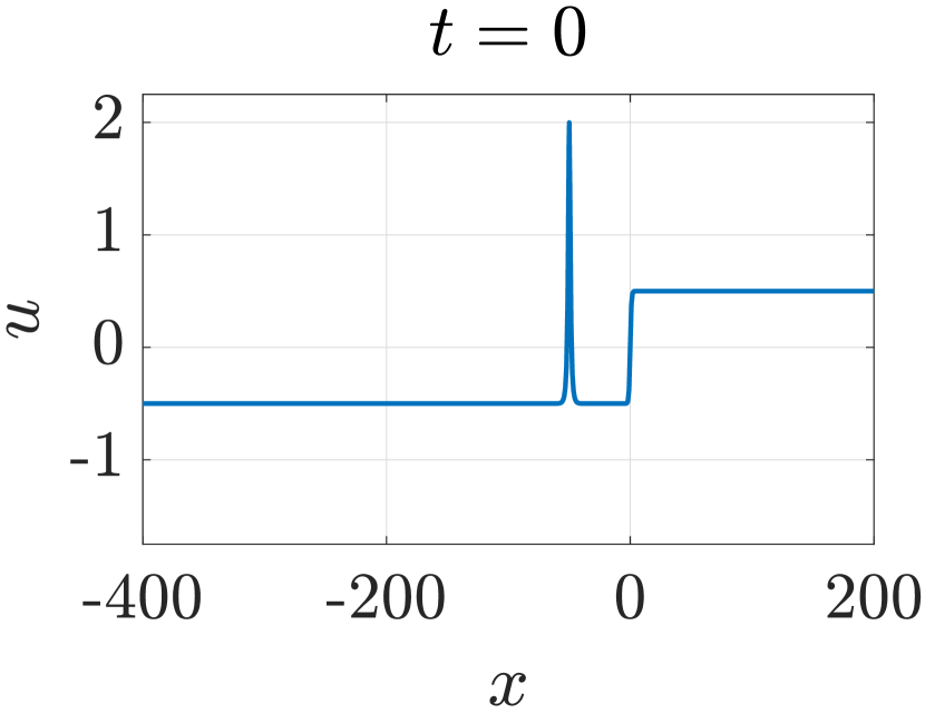
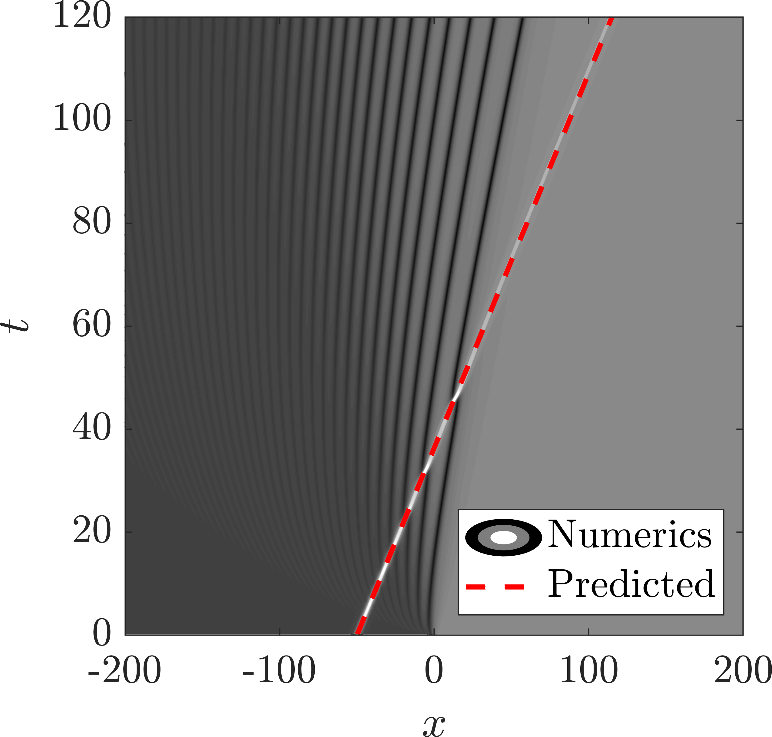
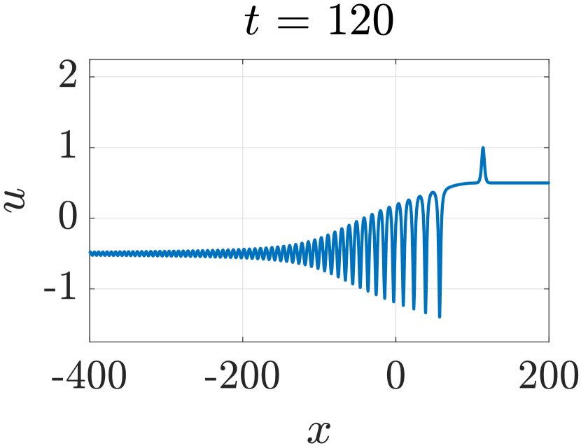
Figure 13: Top, a soliton and CDSW⁺ interaction where $\mu=-1$, $a_{-}=1$, $x_{-}=-50$, $u_{-}=0.5$ and $u_{+}=-0.5$. Bottom, soliton and CDSW^- where $\mu=-1$, $a_{-}=2.5$, $x_{-}=-50$, $u_{-}=-0.5$ and $u_{+}=0.5$.

8.3 Hybrid mean-flows

Regions III, IV, VII and VIII for the Riemann problem result in hybrid mean-flow dynamics involving a CDSW or kink coexisting with a RW or DSW. The analysis for RWs, DSWs and pure kinks and CDSWs serve as the building blocks for determining the soliton tunnelling criterion through these combination flows. We summarise these results for $\mu>0$ in Table 7 and for $\mu<0$ in Table 8.

Direction	Region III - kink$|$RW ($u_{+}>-u_{-}>0$)	Region IV - kink$|$DSW ($u_{-}<-u_{+}<0$)	Region VII - kink$|$RW ($u_{+}<-u_{-}<0$)	Region VIII - kink$|$DSW ($-u_{-}<u_{+}<0$)
$R\to L$	No soliton solutions	No soliton solutions	Tunnelling through RW if $a_{+}>-2u_{-}-2u_{+}$, trapped to the right of the kink	Tunnelling through DSW always, trapped to the right of the kink
$L\to R$	Tunnelling through kink, polarity flips, trapped to the left of the RW	Tunnelling through kink, polarity flips, trapping in DSW if $a_{-}<2u_{+}-2u_{-}$	No soliton solutions	No soliton solutions

Table 7: Results for $\mu>0$ with bright solitons interacting with hybrid mean flows.

Direction	Region III - CDSW$|$RW ($u_{+}>-u_{-}>0$)	Region IV - CDSW$|$DSW ($u_{-}<-u_{+}<0$)	Region VII - CDSW$|$RW ($u_{+}<-u_{-}<0$)	Region VIII - CDSW$|$DSW ($-u_{-}<u_{+}<0$)
$R\to L$	No interaction	Interaction and trapping if $a_{+}<-2u_{+}-2u_{-}$	No interaction	No interaction
$L\to R$	Tunnelling if $a_{-}>2u_{+}-2u_{-}$	Tunnelling if $a_{-}>2u_{+}-2u_{-}$	Tunnelling if $a_{-}>-2u_{+}-2u_{-}$	Tunnelling for any amplitude

Table 8: Results for $\mu<0$ with bright solitons interacting with hybrid mean flows.

9 Kink-mean flow interaction

So far, we have considered the case of solitons interacting with mean flows. Kinks are another localised wave structure that arise as solutions in nonconvex systems, so it is natural to consider their interaction with mean flows. Unlike in soliton-mean flow tunnelling where the mean flow is essentially unchanged by the interaction, in this case, both the kink and the mean flow are significantly altered by the interaction. In addition, we find that the admissibility condition for tunnelling is always satisfied by the kink so there is no trapping.

Kinks occur when $u_{3}\to u_{2}=u_{1}$, causing all three modulation equations in the system (54) to collapse into the dispersionless mean flow equation $\bar{u}_{t}+3\bar{u}^{2}\bar{u}_{x}=0$. The amplitude of the kink is $a=-2\bar{u}$, resulting in $q=0$. Since the kink velocity is slower than the RW or DSW speed, it can only interact from right to left. The kink trajectory is given by

$$\frac{\mathrm{d}x}{\mathrm{d}t}=\bar{u}^{2},\qquad x(0)=x_{+},$$ (101)

which satisfies the Rankine-Hugoniot condition. The kink propagates like a shock.

(i) Kink-RW interaction

The kink trajectory during interaction with a RW is the shock trajectory and can be solved for explicitly using (72) and (101), giving

$$\frac{\mathrm{d}x}{\mathrm{d}t}=\frac{x}{3t},\qquad 3u_{-}^{2}t<x<3u_{+}^{2}t,$$ (102)

with the initial position given by $x_{0}=x_{+}>0$. Numerical experiments verify that this is true, as seen in Fig. 14. As the kink travels through, the RW switches polarity.

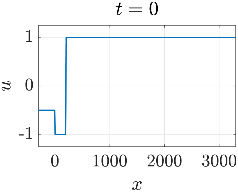
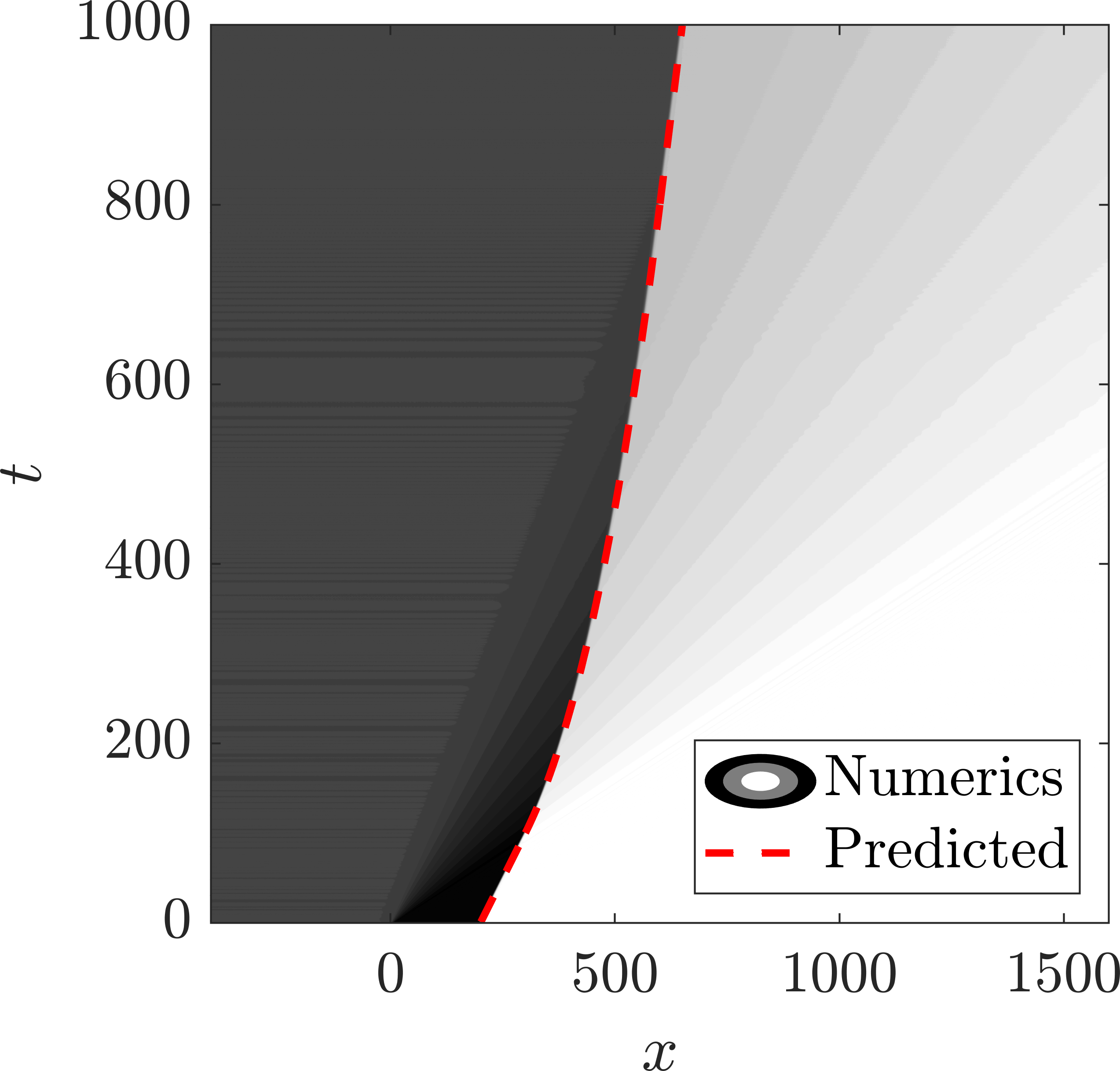
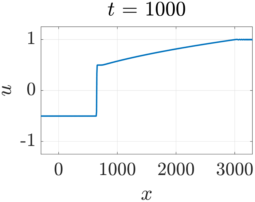
Figure 14: Backward kink-RW interaction with $\mu=1$, $a_{+}=2$, $x_{+}=200$, $u_{-}=-0.5$ and $u_{+}=-1$. The predicted $a_{-}$ is 1 and the predicted $\Delta$ is 200. The numerical solution gives $a_{-}=0.9984$ and $\Delta=199.02$ at $t=1000$.

Again for DSWs, interaction with the kink causes the DSW to switch polarity as seen in the numerical experiment of Fig. 15. These polarity switches are only possible due to nonconvexity. The kink-DSW trajectory is given by eq. (101), where the DSW mean flow $\bar{u}=\bar{u}(x/t)$ is determined by (75), (73) and (74).

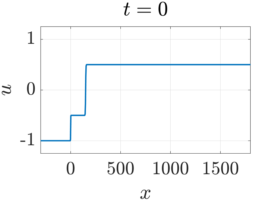
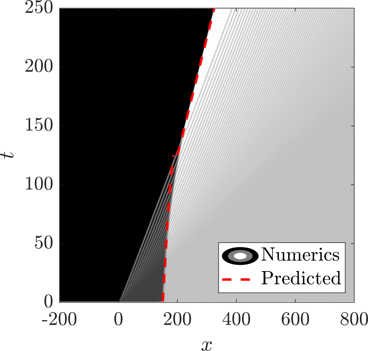
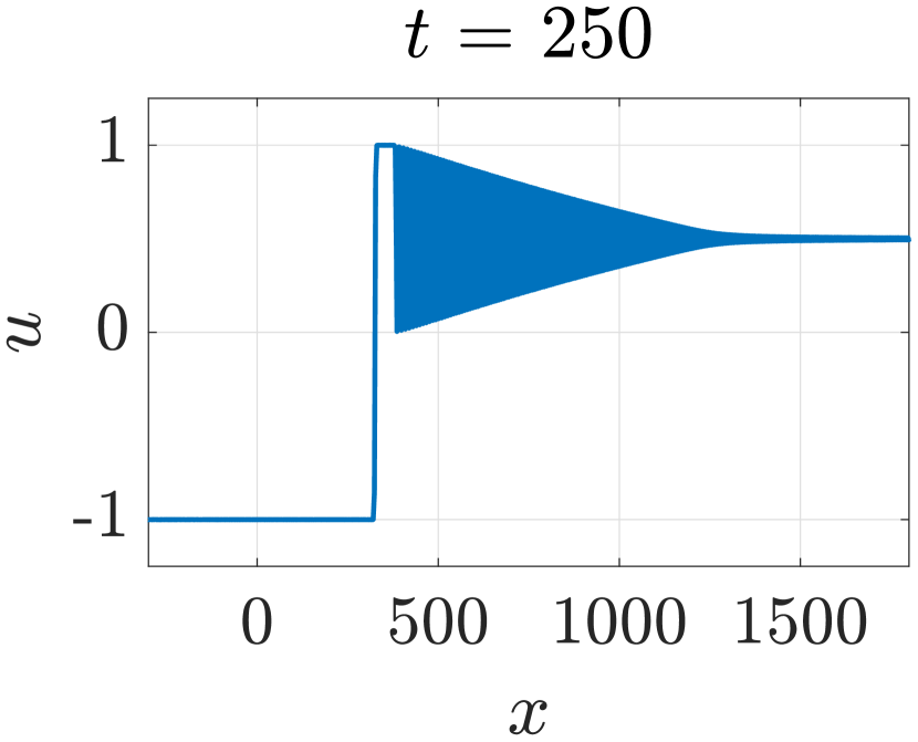
Figure 15: Kink-DSW interaction with $\mu=1$, $a_{+}=1$. $x_{+}=150$, $u_{-}=-1$ and $u_{+}=-0.5$. The predicted $a_{-}$ is 2 and the predicted $\Delta$ is -75. The numerical solution gives $a_{-}=2.0022$ and $\Delta=-74.56$ at $t=250$.

Note that kink-kink interaction is not possible as multiple kinks will co-propagate.

10 Generalisation to arbitrary soliton-convex mean flows

We have described soliton tunnelling interactions specifically with mean flows that emerge from a Riemann step-type initial condition. However, the tunnelling problem can be generalised to determine the phase shift and amplitude of a soliton that tunnels through an arbitrary mean hydrodynamic flow. If tunnelling occurs, only the far field mean flow conditions $u_{-}$ and $u_{+}$ are needed to predict the transmitted soliton amplitude. The phase shift can be calculated by approximating the initial mean flow $\bar{u}(x,0)$ with a series of step functions and taking a limit that results in the Riemann integral

$$\Delta=\left\{\begin{array}[]{ll}\displaystyle\int_{x_{-}}^{x_{0}}\left(\sqrt{\frac{\bar{u}(x,0)^{2}-q^{2}}{u_{-}^{2}-q^{2}}}-1\right)dx,&\text{ assuming }R\to L\\ \displaystyle\int_{x_{0}}^{x_{+}}\left(\sqrt{\frac{\bar{u}(x,0)^{2}-q^{2}}{u_{+}^{2}-q^{2}}}-1\right)dx,&\text{ assuming }L\to R\end{array}\right.$$ (103)

where $x_{0}$ is the initial soliton position and $x_{-}$ or $x_{+}$ is a point where the mean flow has equilibrated to the far field constant.

This phase shift calculation holds only when the system remains strictly hyperbolic, otherwise we have $\bar{u}\to q$ as the soliton travels through the mean flow and trapping will occur. However, this can also be predicted from the far field mean flow conditions, as we have done throughout this work.

Figure 16 depicts a numerical example of a soliton tunnelling through a mean flow that is a combination of a Gaussian and a Riemann step. The predicted trajectory pre and post mean flow interaction shows good agreement with the numerics, as does the transmitted amplitude.

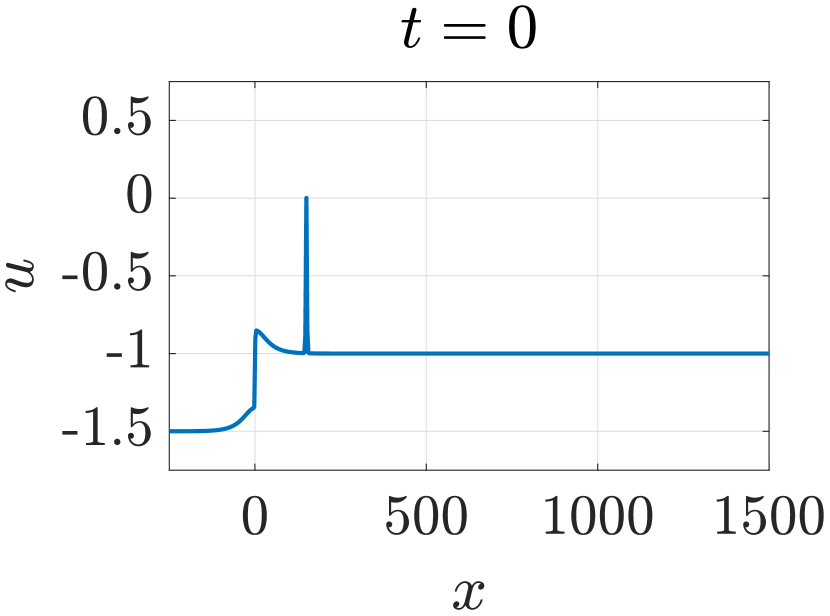
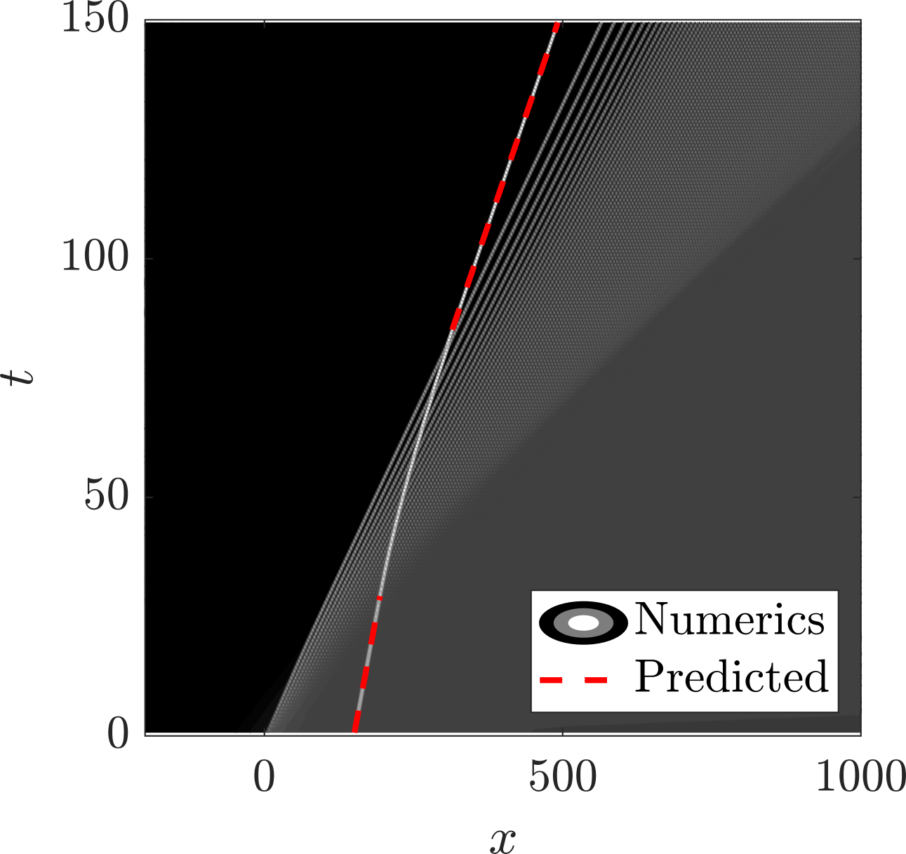
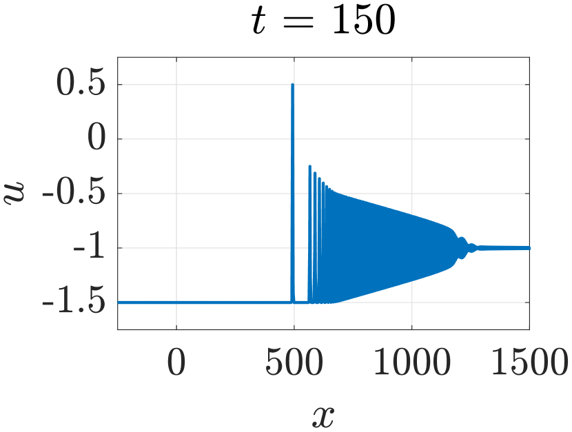
Figure 16: Soliton interaction with an arbitrary mean flow with $\mu=-1$, $x_{+}=150$, $a_{+}=1$, $u_{-}=-1.5$, and $u_{+}=-1$. The predicted amplitude after tunnelling is 2 and the predicted phase shift is -69.28. The numerical result is $a_{-}=2.028$ and $\Delta=-69.24$ at $t=150$.

11 Conclusions and Outlook

In this work, we have investigated the impact of hydrodynamic flux nonconvexity on the relatively new type of soliton-mean flow interaction in which both the soliton and the slowly varying mean flow are governed by the same nonlinear dispersive PDE. The role of mean flows in such solitonic dispersive hydrodynamics is played by either rarefaction waves (RWs) or dispersive shock waves (DSWs). In the latter case, the slowly varying mean flow occurs as a result of averaging over fast, locally periodic nonlinear oscillations of the DSW wave field. This kind of wave-mean flow interaction has been studied previously in the framework of dispersive hydrodynamics described by equations of the Kortweg-de Vries (KdV) type, whose hydrodynamic flux satisfies the convexity property $f^{\prime\prime}(u)\neq 0$ [52, 62].

As a basic model acutely capturing the effects of nonconvex flux on solitonic dispersive hydrodynamics, we used the modified KdV (mKdV) equation, a canonical equation describing, in particular, internal waves in stratified fluids. We considered both focusing and defocusing variants of the mKdV equation, which exhibit rather differing properties in the nonconvex propagation regime. Along with KdV type solitary waves, RWs and DSWs, the mKdV equation supports nonclassical wave structures including kinks, algebraic solitons and contact DSWs [14]. Due to the variety of solitary waves and mean flow configurations, the mKdV equation exhibits a much richer classification of soliton-mean flow interactions than the KdV equation, and more, generally, dispersive hydrodynamics with convex flux.

Multiscale, soliton-mean flow interactions are studied using Whitham modulation theory. An accurate and effective description of soliton-mean flow interactions is achieved by the soliton reduction of the Whitham modulation system, which we formulate in a general form for scalar dispersive hydrodynamics with nonconvex flux. Expanding on the results of [52], we show that the solitonic modulation system with nonconvex flux admits two invariants that yield the amplitude and phase conditions relating the soliton parameters pre and post interaction with the expanding mean flow between distinct boundary states at $\pm\infty$.

One of the main results of our study is the general admissibility criterion for a soliton to tunnel through a mean flow, which is formulated in terms of maintenance of strict hyperbolicity (distinct characteristic speeds) of the solitonic modulation system (8) through the interaction. Conversely, trapping occurs when the characteristics of the solitonic system coalesce.

The general construction of the solitonic modulation system for dispersive hydrodynamics with nonconvex flux is realised for the mKdV equation for both dispersion signs. The nonconvexity of the hydrodynamic flux in the mKdV equation allows for both polarities of solitons and DSWs to exist, no matter the sign of dispersion. This is demonstrated to lead to new, interesting interaction behaviour, which includes soliton polarity reversal as a result of tunnelling through a kink mean flow. On the other hand, kinks are heteroclinic solitary waves that tunnel through DSWs and RW mean flows accompanied by the mean flow’s polarity change.

An important application of this analysis is to the nonlinear dynamics of internal ocean waves, where solitons of both polarities and mean flows such as RWs and DSWs (undular bores) are often observed [1]. Along with the mKdV equation, internal waves can be modelled by the Gardner equation that combines KdV and mKdV hydrodynamic fluxes [22]. The generalisation of our results to the Gardner equation is straightforward. We stress that our approach does not make use of the integrability of the mKdV equation, so can be applied to nonintegrable, nonconvex dispersive hydrodynamics. In particular, a new, intringuing nonconvex scalar model has recently been derived for long-wave potential-vorticity dynamics of coastal fronts in [34]. The study of soliton-mean flow interaction for this model and its fluid dynamic implications would be an interesting and relevant application of the theory presented here.

Our theory can also be extended to bidirectional wave systems describing internal gravity waves in fluids with the Miyata-Choi-Camassa equations [8] being an obvious candidate model. Other applications include polarisation waves in two-component Bose-Einstein condensates [11, 31], nonlinear optics described by nonconvex equations [32, 33] and collisionless plasma [57, 7, 58]. Yet another possible application is in the hydrodynamic interpretation of far-from-equilibrium nonlinear magnetisation dynamics such as in [29], where solitons and DSWs can also emerge.

Future directions include considering dispersion as an additional source of nonconvexity. Such systems are abundant in geophysical fluids, describing magma and glacier flows [59, 63] or wave-ice sheet interactions [30]. Indeed, recent works on DSWs in systems with nonconvex dispersion [51, 17, 61, 27, 3, 10] reveal a plethora of unusual behaviours that can lead to new, interesting soliton-mean flow interactions.

References

- [1] J. R. Apel. Oceanic internal waves and solitons. Prepared for Office of Naval Research Code 322 PO, Global Ocean Associates, 2002.
- [2] John R. Apel, Lev A. Ostrovsky, Yury A. Stepanyants, and James F. Lynch. Internal solitons in the ocean and their effect on underwater sound. The Journal of the Acoustical Society of America, 121(2):695, 2007.
- [3] Saleh Baqer and Noel F. Smyth. Modulation theory and resonant regimes for dispersive shock waves in nematic liquid crystals. Physica D: Nonlinear Phenomena, 403:132334, February 2020.
- [4] R. F. Bikbaev. Korteweg-de Vries equation with finite-gap boundary conditions, and the Whitham deformations of Riemann surfaces. Funct Anal Its Appl, 23(4):257–266, October 1989.
- [5] Gino Biondini and Jonathan Lottes. Nonlinear interactions between solitons and dispersive shocks in focusing media. Physical Review E, 99(2), February 2019.
- [6] Oliver Bühler. Waves and Mean Flows. Cambridge Monographs on Mechanics. Cambridge University Press, 2009.
- [7] G. Chanteur and M. Raadu. Formation of shocklike modified Korteweg–de Vries solitons: Application to double layers. Physics of Fluids, 30(9):2708–2719, September 1987.
- [8] Wooyoung Choi and Roberto Camassa. Fully nonlinear internal waves in a two-fluid system. Journal of Fluid Mechanics, 396:1–36, 1999.
- [9] T. Congy, G. A. El, and M. A. Hoefer. Interaction of linear modulated waves and unsteady dispersive hydrodynamic states with application to shallow water waves. Journal of Fluid Mechanics, 875:1145–1174, September 2019.
- [10] T. Congy, G. A. El, M. A. Hoefer, and M. Shearer. Dispersive Riemann problem for the Benjamin-Bona-Mahony equation. arXiv:2012.14579 [nlin], December 2020. arXiv: 2012.14579.
- [11] T. Congy, A. M. Kamchatnov, and N. Pavloff. Nonlinear waves in coherently coupled Bose-Einstein condensates. Physical Review A, 93(4), April 2016.
- [12] Constantine M. Dafermos. Hyperbolic Conservation Laws in Continuum Physics. Springer, Berlin, 4th ed. edition, 2016.
- [13] C. F. Driscoll and T. M. O’Neil. Modulational instability of cnoidal wave solutions of the modified Korteweg–de Vries equation. Journal of Mathematical Physics, 17(7):1196–1200, 1975.
- [14] G. El, M. Hoefer, and M. Shearer. Dispersive and Diffusive-Dispersive Shock Waves for Nonconvex Conservation Laws. SIAM Rev., 59(1):3–61, January 2017.
- [15] G. A. El. Resolution of a shock in hyperbolic systems modified by weak dispersion. Chaos, 15:037103, 2005.
- [16] G. A. El and M. A. Hoefer. Dispersive shock waves and modulation theory. Physica D: Nonlinear Phenomena, 333:11–65, October 2016.
- [17] Gennady A. El and Noel F. Smyth. Radiating dispersive shock waves in non-local optical media. Proceedings of the Royal Society A: Mathematical, Physical and Engineering Science, 472(2187):20150633, March 2016.
- [18] J. G. Esler and J. D. Pearce. Dispersive dam-break and lock-exchange flows in a two-layer fluid. Journal of Fluid Mechanics, 667:555–585, 2011.
- [19] H. Flaschka, M. G. Forest, and D. W. McLaughlin. Multiphase averaging and the inverse spectral solution of the Korteweg-de Vries equation. Comm. Pure Appl. Math., 33:739–784, 1980.
- [20] Tamara Grava and Alexader Minakov. On the long time asymptotic of the modified Korteweg de Vries equation with step-like initial data. arXiv:1907.11859 [math-ph, physics:nlin], July 2019. arXiv: 1907.11859.
- [21] R. Grimshaw. Slowly varying solitary waves. I. Korteweg-de Vries equation. Proc. R. Soc. Lond. A, 368:359–375, 1979.
- [22] R. H. J. Grimshaw. Internal solitary waves. In R. H. J. Grimshaw, editor, Environmental Stratified Flows, pages 1–27. Kluwer, 2002.
- [23] A. V. Gurevich, A. L. Krylov, and G. A. El. Nonlinear modulated waves in dispersive hydrodynamics. Sov. Phys. JETP, 71(5):899–910, 1990.
- [24] A. V. Gurevich and L. P. Pitaevskii. Nonstationary structure of a collisionless shock wave. Sov. Phys. JETP, 38(2):291–297, 1974. Translation from Russian of A. V. Gurevich and L. P. Pitaevskii, Zh. Eksp. Teor. Fiz. 65, 590-604 (August 1973).
- [25] Brian Hayes and Michael Shearer. Undercompressive shocks and Riemann problems for scalar conservation laws with non-convex fluxes. Proceedings of the Royal Society of Edinburgh, Section: A Mathematics, 129(04):733–754, 1999.
- [26] Karl R. Helfrich and W. Kendall Melville. Long nonlinear internal waves. Annu. Rev. Fluid Mech., 38:395–425, 2006.
- [27] Mark A. Hoefer, Noel F. Smyth, and Patrick Sprenger. Modulation theory solution for nonlinearly resonant, fifth-order Korteweg-de Vries, nonclassical, traveling dispersive shock waves. Studies in Applied Mathematics, 142(3):219–240, April 2019.
- [28] Peter E. Holloway, Efim Pelinovsky, and Tatjana Talipova. A generalized Korteweg-de Vries model of internal tide transformation in the coastal zone. Journal of Geophysical Research: Oceans, 104(C8):18333–18350, August 1999.
- [29] Ezio Iacocca, T. J. Silva, and Mark A. Hoefer. Breaking of Galilean Invariance in the Hydrodynamic Formulation of Ferromagnetic Thin Films. Physical Review Letters, 118(1), January 2017.
- [30] Andrej Teimurazovich Il’ichev and V. Ya Tomashpolskii. Soliton-like structures on a liquid surface under an ice cover. Theoretical and Mathematical Physics, 182(2):231–245, 2015.
- [31] S. K. Ivanov, A. M. Kamchatnov, T. Congy, and N. Pavloff. Solution of the Riemann problem for polarization waves in a two-component Bose-Einstein condensate. Physical Review E, 96(6):062202, December 2017.
- [32] Sergey K Ivanov. Riemann problem for the light pulses in optical fibers for the generalized Chen-Lee-Liu equation. Physical Review A, 101(5):053844, 2020.
- [33] Sergey K Ivanov and Anatoly M. Kamchatnov. Riemann problem for the photon fluid: Self-steepening effects. Physical Review A, 96(5):053827, 2017.
- [34] S. Jamshidi and E. R. Johnson. The long-wave potential-vorticity dynamics of coastal fronts. Journal of Fluid Mechanics, 888:A19, 2020.
- [35] Tsunehiko Kakutani and Nobuyoshi Yamasaki. Solitary Waves on a Two-Layer Fluid. J. Phys. Soc. Jpn., 45(2):674–679, August 1978.
- [36] A M Kamchatnov. Evolution of initial discontinuities in the DNLS equation theory. Journal of Physics Communications, 2(2):025027, February 2018.
- [37] A. M. Kamchatnov, Y.-H. Kuo, T.-C. Lin, T.-L. Horng, S.-C. Gou, R. Clift, G. A. El, and R. H. J. Grimshaw. Undular bore theory for the Gardner equation. Physical Review E, 86(3):036605, September 2012.
- [38] A. M. Kamchatnov, Y.-H. Kuo, T.-C. Lin, T.-L. Horng, S.-C. Gou, R. Clift, G. A. El, and R. H. J. Grimshaw. Transcritical flow of a stratified fluid over topography: analysis of the forced Gardner equation. Journal of Fluid Mechanics, 736:495–531, November 2013.
- [39] A M Kamchatnov, A Spire, and V V Konotop. On dissipationless shock waves in a discrete nonlinear Schrödinger equation. Journal of Physics A: Mathematical and General, 37(21):5547–5568, May 2004.
- [40] Y S Kivshar and B A Malomed. Dynamics of solitons in nearly integrable systems. Rev Mod Phys, 61:763, 1989.
- [41] Alfred Kluwick, Stefan Scheichl, and Edward A. Cox. Near-critical hydraulic flows in two-layer fluids. Journal of Fluid Mechanics, 575:187, March 2007.
- [42] Yuji Kodama, V. U. Pierce, and Fei-Ran Tian. On the Whitham Equations for the Defocusing Complex Modified KdV Equation. SIAM Journal on Mathematical Analysis, 40(5):1750–1782, January 2009.
- [43] V. Kotlyarov and A. Minakov. Step-initial function to the mKdV equation: hyper-elliptic long-time asymptotics of the solution. Journal of Mathematical Physics, Analysis, Geometry, 8(1):38–62, 2012.
- [44] Vladimir Kotlyarov and Alexander Minakov. Riemann–Hilbert problem to the modified Korteveg–de Vries equation: Long-time dynamics of the steplike initial data. Journal of Mathematical Physics, 51(9):093506, 2010.
- [45] P. D. Lax. Hyperbolic systems of conservation laws and the mathematical theory of shock waves. SIAM, 1973.
- [46] J. A. Leach. An initial-value problem for the modified Korteweg-de Vries equation. IMA Journal of Applied Mathematics, 78(6):1196–1213, December 2013.
- [47] J.A. Leach. An initial-value problem for the defocusing modified Korteweg–de Vries equation. Journal of Differential Equations, 252(2):1032–1051, January 2012.
- [48] P. G. LeFloch. Hyperbolic systems of conservation laws. Birkhauser, 2002.
- [49] C.D. Levermore. The hyperbolic nature of the zero dispersion KdV limit. Commun. Part. Diff. Eq., 13(4):495–514, 1988.
- [50] Lan Li, Caixia Wang, and Roger Grimshaw. Observation of internal wave polarity conversion generated by a rising tide. Geophysical Research Letters, 42(10):4007–4013, May 2015.
- [51] Nicholas K. Lowman and M. A. Hoefer. Dispersive shock waves in viscously deformable media. Journal of Fluid Mechanics, 718:524–557, 2013.
- [52] Michelle D. Maiden, Dalton V. Anderson, Nevil A. Franco, Gennady A. El, and Mark A. Hoefer. Solitonic Dispersive Hydrodynamics: Theory and Observation. Physical Review Letters, 120(14):144101, April 2018.
- [53] T.R. Marchant. Undular bores and the initial-boundary value problem for the modified Korteweg-de Vries equation. Wave Motion, 45(4):540–555, March 2008.
- [54] Chiang C. Mei, Michael Stiassnie, and Dick K.-P. Yue. Theory and applications of ocean surface waves. Number Volume 23 in Advanced Series on Ocean Engineering. World Scientific, Hackensack, N.J, 2005.
- [55] Robert M. Miura. Korteweg‐de Vries Equation and Generalizations. I. A Remarkable Explicit Nonlinear Transformation. Journal of Mathematical Physics, 9(8):1202–1204, August 1968.
- [56] M. Miyata. An internal solitary wave of large amplitude. La Mer, 23(2):43–48, 1985.
- [57] Y. Nakamura, J. L. Ferreira, and G. O. Ludwig. Experiments on ion-acoustic rarefactive solitons in a multi-component plasma with negative ions. Journal of plasma physics, 33(02):237–248, 1985.
- [58] Michael S. Ruderman, Tatyana Talipova, and Efim Pelinovsky. Dynamics of modulationally unstable ion-acoustic wavepackets in plasmas with negative ions. Journal of Plasma Physics, 74(05):639–656, April 2008.
- [59] David R. Scott, David J. Stevenson, and John A. Whitehead. Observations of solitary waves in a viscously deformable pipe. Nature, 319(6056):759–761, February 1986.
- [60] E L Shroyer, J N Moum, and J D Nash. Observations of Polarity Reversal in Shoaling Nonlinear Internal Waves. JOURNAL OF PHYSICAL OCEANOGRAPHY, page 10, 2008.
- [61] P. Sprenger and M. Hoefer. Shock Waves in Dispersive Hydrodynamics with Nonconvex Dispersion. SIAM J. Appl. Math., 77:26–50, January 2017.
- [62] P. Sprenger, M. A. Hoefer, and G. A. El. Hydrodynamic optical soliton tunneling. Physical Review E, 97(3), March 2018.
- [63] Aaron G. Stubblefield, Marc Spiegelman, and Timothy T. Creyts. Solitary waves in power-law deformable conduits with laminar or turbulent fluid flow. Journal of Fluid Mechanics, 886:A10, March 2020.
- [64] G. B. Whitham. Non-linear dispersive waves. Proc. Roy. Soc. Ser. A, 283:238–261, 1965.
- [65] G. B. Whitham. Linear and nonlinear waves. Wiley, New York, 1974.
- [66] Guoqiang Zhang and Zhenya Yan. Focusing and defocusing mKdV equations with nonzero boundary conditions: Inverse scattering transforms and soliton interactions. Physica D: Nonlinear Phenomena, 410:132521, September 2020.