Optimal Approximation Rate of ReLU Networks in terms of Width and Depth

Abstract

This paper concentrates on the approximation power of deep feed-forward neural networks in terms of width and depth. It is proved by construction that ReLU networks with width $\mathcal{O}\big{(}\max\{d\lfloor N^{1/d}\rfloor,\,N+2\}\big{)}$ and depth $\mathcal{O}(L)$ can approximate a Hölder continuous function on $[0,1]^{d}$ with an approximation rate $\mathcal{O}\big{(}\lambda\sqrt{d}(N^{2}L^{2}\ln N)^{-\alpha/d}\big{)}$, where $\alpha\in(0,1]$ and $\lambda>0$ are Hölder order and constant, respectively. Such a rate is optimal up to a constant in terms of width and depth separately, while existing results are only nearly optimal without the logarithmic factor in the approximation rate. More generally, for an arbitrary continuous function $f$ on $[0,1]^{d}$, the approximation rate becomes $\mathcal{O}\big{(}\,\sqrt{d}\,\omega_{f}\big{(}(N^{2}L^{2}\ln N)^{-1/d}\big{)}\,\big{)}$, where $\omega_{f}(\cdot)$ is the modulus of continuity. We also extend our analysis to any continuous function $f$ on a bounded set. Particularly, if ReLU networks with depth $31$ and width $\mathcal{O}(N)$ are used to approximate one-dimensional Lipschitz continuous functions on $[0,1]$ with a Lipschitz constant $\lambda>0$, the approximation rate in terms of the total number of parameters, $W=\mathcal{O}(N^{2})$, becomes $\mathcal{O}(\tfrac{\lambda}{W\ln W})$, which has not been discovered in the literature for fixed-depth ReLU networks.

Key words. Deep ReLU Networks; Optimal Approximation; VC-dimension; Bit Extraction.

1 Introduction

Over the past few decades, the expressiveness of neural networks has been widely studied from many points of view, e.g., in terms of combinatorics [27], topology [4], Vapnik-Chervonenkis (VC) dimension [3, 31, 13], fat-shattering dimension [19, 1], information theory [30], classical approximation theory [6, 16, 2, 41, 32, 44, 33, 24, 34, 32, 35, 20, 36, 10], optimization [17, 29, 18, 14, 21]. The error analysis of neural networks consists of three parts: the approximation error, the optimization error, and the generalization error. This paper focuses on the approximation error for ReLU networks.

The approximation errors of feed-forward neural networks with various activation functions have been studied for different types of functions, e.g., smooth functions [25, 22, 40, 9, 24], piecewise smooth functions [30], band-limited functions [26], continuous functions [41, 33, 34, 35]. In the early works of approximation theory for neural networks, the universal approximation theorem [6, 15, 16] without approximation rates showed that there exists a sufficiently large neural network approximating a target function in a certain function space within any given error $\varepsilon>0$. In particular, it is shown in [23] that the ReLU-activated residual neural network with one-neuron hidden layers is a universal approximator. The universal approximation property for general residual neural networks was proved in [20] via a dynamical system approach.

An asymptotic analysis of the approximation rate in terms of depth is provided in [41, 43] for ReLU networks. To be exact, the nearly optimal approximation rates of ReLU networks with width ${\mathcal{O}}(d)$ and depth ${\mathcal{O}}(L)$ for functions in $C([0,1]^{d})$ and the unit ball of $C^{s}([0,1]^{d})$ are ${\mathcal{O}}(\omega_{f}(L^{-2/d}))$ and ${\mathcal{O}}((L/\ln L)^{-2s/d})$, respectively. These two papers provide the approximation rate in terms of depth asymptotically for fixed-width networks. A different approach is used in [33, 24] to obtain a quantitative characterization of the approximation rate in terms of width, depth, and smoothness order for continuous and smooth functions.

Particularly, it was shown in [33] that a ReLU network with width $C_{1}(d)\cdot N$ and depth $C_{2}(d)\cdot L$ can attain an approximation error $C_{3}(d)\cdot\omega_{f}(N^{-2/d}L^{-2/d})$ to approximate a continuous function $f$ on $[0,1]^{d}$, where $C_{1}(d)$, $C_{2}(d)$, and $C_{3}(d)$ are three constants in $d$ with explicit formulas to specify their values, and $\omega_{f}(\cdot)$ is the modulus of continuity of $f\in C([0,1]^{d})$ defined via

$$\omega_{f}(r)\coloneqq\sup\big{\{}|f(\bm{x})-f(\bm{y})|:\bm{x},\bm{y}\in[0,1]^{d},\ \|\bm{x}-\bm{y}\|_{2}\leq r\big{\}},\quad\textnormal{for any $r\geq 0$}.$$

Such an approximation error is optimal in terms of $N$ and $L$ up to a logarithmic term and the corresponding optimal approximation theory is still unavailable. To address this problem, we provide a constructive proof in this paper to show that ReLU networks of width ${\mathcal{O}}(N)$ and depth ${\mathcal{O}}(L)$ can approximate an arbitrary continuous function $f$ on $[0,1]^{d}$ with an optimal approximation error ${\mathcal{O}}\left(\sqrt{d}\,\omega_{f}\big{(}(N^{2}L^{2}\ln N)^{-1/d}\big{)}\right)$ in terms of $N$ and $L$. As shown by our main result, Theorem 1.1 below, the approximation rate obtained here admits explicit formulas to specify its prefactors when $\omega_{f}(\cdot)$ is known.

Theorem 1.1.

Given a continuous function $f\in C([0,1]^{d})$, for any $N\in\mathbb{N}^{+}$, $L\in\mathbb{N}^{+}$, and $p\in[1,\infty]$, there exists a function $\phi$ implemented by a ReLU network with width $C_{1}\max\big{\{}d\lfloor N^{1/d}\rfloor,\,N+2\big{\}}$ and depth $11L+C_{2}$ such that

$$\|f-\phi\|_{L^{p}([0,1]^{d})}\leq 131\sqrt{d}\,\omega_{f}\Big{(}\big{(}N^{2}L^{2}\log_{3}(N+2)\big{)}^{-1/d}\Big{)},$$

where $C_{1}=16$ and $C_{2}=18$ if $p\in[1,\infty)$; $C_{1}=3^{d+3}$ and $C_{2}=18+2d$ if $p=\infty$.

Note that $3^{d+3}\max\big{\{}d\lfloor N^{1/d}\rfloor,\,N+2\big{\}}\leq 3^{d+3}\max\big{\{}dN,\,3N\big{\}}\leq 3^{d+4}dN$. Given any ${\widetilde{N}},{\widetilde{L}}\in\mathbb{N}^{+}$ with ${\widetilde{N}}\geq 3^{d+4}d$ and ${\widetilde{L}}\geq 29+2d$, there exist $N,L\in\mathbb{N}^{+}$ such that

$$3^{d+4}dN\leq{\widetilde{N}}<3^{d+4}d(N+1)\textnormal{\quad and\quad}11L+18+2d\leq{\widetilde{L}}<11(L+1)+18+2d.$$

It follows that

$$N\geq\frac{N+1}{3}>\frac{{\widetilde{N}}}{3^{d+5}d}\textnormal{\quad and\quad}L\geq\frac{L+1}{2}>\frac{1}{2}\cdot\frac{{\widetilde{L}}-18-2d}{11}=\frac{{\widetilde{L}}-18-2d}{22}.$$

Then we have an immediate corollary of Theorem 1.1.

Corollary 1.2.

Given a continuous function $f\in C([0,1]^{d})$, for any ${\widetilde{N}}\in\mathbb{N}^{+}$ and ${\widetilde{L}}\in\mathbb{N}^{+}$ with ${\widetilde{N}}\geq 3^{d+4}d$ and ${\widetilde{L}}\geq 29+2d$, there exists a function $\phi$ implemented by a ReLU network with width ${\widetilde{N}}$ and depth ${\widetilde{L}}$ such that

$$\|f-\phi\|_{L^{\infty}([0,1]^{d})}\leq 131\sqrt{d}\,\omega_{f}\bigg{(}\Big{(}(\tfrac{{\widetilde{N}}}{3^{d+5}d})^{2}(\tfrac{{\widetilde{L}}-18-2d}{22})^{2}\log_{3}(\tfrac{{\widetilde{N}}}{3^{d+5}d}+2)\Big{)}^{-1/d}\bigg{)}.$$

As a special case of Theorem 1.1 for explicit error characterization, let us take Hölder continuous functions as an example. Let ${\textnormal{H\"{o}lder}([0,1]^{d},\alpha,\lambda)}$ denote the space of Hölder continuous functions on $[0,1]^{d}$ of order $\alpha\in(0,1]$ with a Hölder constant $\lambda>0$. We have an immediate corollary of Theorem 1.1 as follows.

Corollary 1.3.

Given a Hölder continuous function $f\in{\textnormal{H\"{o}lder}([0,1]^{d},\alpha,\lambda)}$, for any $N\in\mathbb{N}^{+}$, $L\in\mathbb{N}^{+}$, and $p\in[1,\infty]$, there exists a function $\phi$ implemented by a ReLU network with width $C_{1}\max\big{\{}d\lfloor N^{1/d}\rfloor,\,N+2\big{\}}$ and depth $11L+C_{2}$ such that

$$\|f-\phi\|_{L^{p}([0,1]^{d})}\leq 131\lambda\sqrt{d}\big{(}N^{2}L^{2}\log_{3}(N+2)\big{)}^{-\alpha/d},$$

where $C_{1}=16$ and $C_{2}=18$ if $p\in[1,\infty)$; $C_{1}=3^{d+3}$ and $C_{2}=18+2d$ if $p=\infty$.

To better illustrate the importance of our theory, we summarize our key contributions as follows.

1. Upper bound: We provide a quantitative and non-asymptotic approximation rate $131\sqrt{d}\,\omega_{f}\Big{(}\big{(}N^{2}L^{2}\log_{3}(N+2)\big{)}^{-1/d}\Big{)}$ in terms of width ${\mathcal{O}}(N)$ and depth ${\mathcal{O}}(L)$ for any $f\in C([0,1]^{d})$ in Theorem 1.1.

   1. This approximation error analysis can be extended to $f\in C(E)$ for any $E\subseteq[-R,R]^{d}$ with $R>0$ as we shall see later in Theorem 2.5.

   2. In the case of one-dimensional Lipschitz continuous functions on $[0,1]$ with a Lipschitz constant $\lambda>0$, the approximation rate in Theorem 1.1 becomes $\mathcal{O}(\tfrac{\lambda}{W\ln W})$ for ReLU networks with $31$ hidden layers and $\mathcal{O}(W)$ parameters via setting $L=1$ and $W={\mathcal{O}}(N^{2})$ therein. To the best of our knowledge, the approximation rate $\mathcal{O}(\tfrac{\lambda}{W\ln W})$ is better than existing known results using fixed-depth ReLU networks to approximate Lipschitz continuous functions on $[0,1]$.

2. Lower bound: Through the VC-dimension bounds of ReLU networks given in [13], we show, in Section 2.3, that the approximation rate $131\lambda\sqrt{d}\big{(}N^{2}L^{2}\log_{3}(N+2)\big{)}^{-\alpha/d}$ in terms of width ${\mathcal{O}}(N)$ and depth ${\mathcal{O}}(L)$ for ${\textnormal{H\"{o}lder}([0,1]^{d},\alpha,\lambda)}$ is optimal as follows.

   1. When the width is fixed, both the approximation upper and lower bounds take the form of $CL^{-2\alpha/d}$ for a positive constant $C$.

   2. When the depth is fixed, both the approximation upper and lower bounds take the form of $C(N^{2}\ln N)^{-\alpha/d}$ for a positive constant $C$.

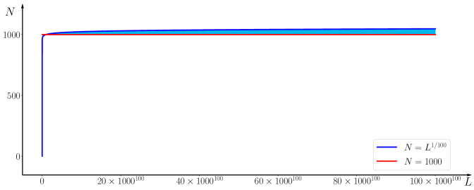
Figure 1: Our rate is optimal in terms of width ${\mathcal{O}}(N)$ and depth ${\mathcal{O}}(L)$ simultaneously except for the region marked in cyan characterized by $\{(N,L)\in\mathbb{N}^{2}:C_{1}\leq N\leq L^{C_{2}}\}$, where $C_{i}=C_{i}(\alpha,d)$ for $i=1,2$ are two positive constants. This figure is an example for $C_{1}=1000$ and $C_{2}=1/100$.

We would like to point out that if $N$ and $L$ vary simultaneously, the rate is optimal in the $N$-$L$ plane except for a small region as shown in Figure 1. See Section 2.3 for a detailed discussion. The earlier result in [33] provides a nearly optimal approximation error that has a gap (a logarithmic term) between the lower and upper bounds. It is technically challenging to match the upper bound with the lower bound. Compared to the nearly optimal rate $19\lambda\sqrt{d}N^{-2\alpha/d}L^{-2\alpha/d}$ for Hölder continuous functions in ${\textnormal{H\"{o}lder}([0,1]^{d},\alpha,\lambda)}$ in [33], this paper achieves the optimal rate $131\lambda\sqrt{d}\big{(}N^{2}L^{2}\log_{3}(N+2)\big{)}^{-\alpha/d}$ using more technical and sophisticated construction. For example, a novel bit extraction technique different to that in [3] is proposed, and new ReLU networks are constructed to approximate step functions more efficiently than those in [33]. The optimal result obtained in this paper could also be extended to other functions spaces, leading to better understanding of deep network approximation.

We have obtained the optimal approximation rate for (Hölder) continuous functions approximated by ReLU networks. There are two possible directions to improve the approximation rate or reduce the effect of the curse of dimensionality. The first one is to consider proper target function spaces, e.g., Barron spaces [2, 8, 12, 37], band-limited functions [5, 26], smooth functions [43, 24], and analytic functions [9]. The other direction is to consider neural networks with other activation functions. For example, the results of [43] imply that $(\sin,\textnormal{ReLU})$-activated networks with $W$ parameters can achieve an asymptotic approximation error ${\mathcal{O}}(2^{-c_{d}\sqrt{W}})$ for Lipschitz continuous functions defined on $[0,1]^{d}$, where $c_{d}$ is an unknown constant depending on $d$. Floor-ReLU networks with width ${\mathcal{O}}(N)$ and depth ${\mathcal{O}}(L)$ are constructed in [34] to admit an approximation rate $\omega_{f}(\sqrt{d}N^{-\sqrt{L}})+2\omega_{f}(\sqrt{d})N^{-\sqrt{L}}$ for any continuous function $f\in C([0,1]^{d})$. It is shown in [35] that three-hidden-layer networks with ${\mathcal{O}}(W)$ parameters using the floor function ($\lfloor x\rfloor)$, the exponential function ($2^{x}$), and the step function (${\mathds{1}}_{x\geq 0}$) as activation functions can approximate Lipschitz functions defined on $[0,1]^{d}$ with an exponentially small error ${\mathcal{O}}(\sqrt{d}2^{-W})$. By the use of more sophisticated activation functions instead of those used in [34, 35, 43], a recent paper [42] shows that there exists a network of size depending on $d$ implicitly, achieving an arbitrary approximation error for any continuous function in $C([0,1]^{d})$. A key ingredient of the approaches mentioned above is to use more than one activation functions to design neural network architectures.

The error analysis of deep learning is to estimate approximation, generalization, and optimization errors. Here, we give a brief discussion, the interested reader can find more details in [24, 34]. Let $\phi(\bm{x};\bm{\theta})$ denote a function computed by a network parameterized with $\bm{\theta}$. Given a target function $f$, the final goal is to find the expected risk minimizer

$$\bm{\theta}_{\mathcal{D}}\coloneqq\operatorname*{arg\,min}_{\bm{\theta}}R_{\mathcal{D}}(\bm{\theta}),\quad\textnormal{where}\ R_{\mathcal{D}}(\bm{\theta})\coloneqq\mathbb{E}_{\bm{x}\sim U(\mathcal{X})}\left[\ell(\phi(\bm{x};\bm{\theta}),f(\bm{x}))\right],$$

with a loss function $\ell(\cdot,\cdot)$ and an unknown data distribution $U(\mathcal{X})$.

In practice, for given samples $\{(\bm{x}_{i},f(\bm{x}_{i}))\}_{i=1}^{n}$, the goal of supervised learning is to identify the empirical risk minimizer

$$\bm{\theta}_{\mathcal{S}}\coloneqq\operatorname*{arg\,min}_{\bm{\theta}}R_{\mathcal{S}}(\bm{\theta}),\quad\textnormal{where}\ R_{\mathcal{S}}(\bm{\theta}):=\frac{1}{n}\sum_{i=1}^{n}\ell\big{(}\phi(\bm{x}_{i};\bm{\theta}),f(\bm{x}_{i})\big{)}.$$

In fact, one could only get a numerical minimizer $\bm{\theta}_{\mathcal{N}}$ via a numerical optimization method. The discrepancy between the target function $f$ and the learned function $\phi(\bm{x};\bm{\theta}_{\mathcal{N}})$ is measured by $R_{\mathcal{D}}(\bm{\theta}_{\mathcal{N}})$, which is bounded by

This paper deals with the approximation error of ReLU networks for continuous functions and gives an upper bound of $R_{\mathcal{D}}(\bm{\theta}_{\mathcal{D}})$ which is optimal up to a constant. Note that the approximation error analysis given here is independent of data samples and deep learning algorithms. However, the analysis of optimization and generalization errors do depend on data samples, deep learning algorithms, models, etc. For example, refer to [28, 8, 7, 11, 17, 29, 18, 14, 21] for a further understanding of the generalization and optimization errors.

The rest of this paper is organized as follows. In Section 2, we prove Theorem 1.1 by assuming Theorem 2.1 is true, show the optimality of Theorem 1.1, and extend our analysis to continuous functions defined on any bounded set. Next, Theorem 2.1 is proved in Section 3 based on Propositions 3.1 and 3.2, the proofs of which can be found in Section 4. Finally, Section 5 concludes this paper with a short discussion.

2 Theoretical analysis

In this section, we first prove Theorem 1.1 and discuss its optimality. Next, we extend our analysis to general continuous functions defined on any bounded set. Notations throughout this paper are summarized in Section 2.1.

2.1 Notations

Let us summarize all basic notations used in this paper as follows.

• Let $\mathbb{R}$, $\mathbb{Q}$, and $\mathbb{Z}$ denote the set of real numbers, rational numbers, and integers, respectively.

• Let $\mathbb{N}$ and $\mathbb{N}^{+}$ denote the set of natural numbers and positive natural numbers, respectively. That is, $\mathbb{N}^{+}=\{1,2,3,\cdots\}$ and $\mathbb{N}=\mathbb{N}^{+}\bigcup\{0\}$.

• Matrices are denoted by bold uppercase letters. For instance, $\bm{A}\in\mathbb{R}^{m\times n}$ is a real matrix of size $m\times n$, and $\bm{A}^{T}$ denotes the transpose of $\bm{A}$. Vectors are denoted as bold lowercase letters. For example, $\bm{v}=[v_{1},\cdots,v_{d}]^{T}=\left[\begin{array}[]{c}v_{1}\\ \vdots\\ v_{d}\end{array}\right]\in\mathbb{R}^{d}$ is a column vector with $\bm{v}(i)=v_{i}$ being the $i$-th element. Besides, “[” and “]” are used to partition matrices (vectors) into blocks, e.g., $\bm{A}=\left[\begin{smallmatrix}\bm{A}_{11}&\bm{A}_{12}\\ \bm{A}_{21}&\bm{A}_{22}\end{smallmatrix}\right]$.

• For any $p\in[1,\infty)$, the $p$-norm (or $\ell^{p}$-norm) of a vector ${\bm{x}}=[x_{1},x_{2},\cdots,x_{d}]^{T}\in\mathbb{R}^{d}$ is defined by

  $$\|{\bm{x}}\|_{p}\coloneqq\big{(}|x_{1}|^{p}+|x_{2}|^{p}+\cdots+|x_{d}|^{p}\big{)}^{1/p}.$$

• For any $x\in\mathbb{R}$, let $\lfloor x\rfloor:=\max\{n:n\leq x,\ n\in\mathbb{Z}\}$ and $\lceil x\rceil:=\min\{n:n\geq x,\ n\in\mathbb{Z}\}$.

• Assume $\bm{n}\in\mathbb{N}^{d}$, then $f(\bm{n})=\mathcal{O}(g(\bm{n}))$ means that there exists positive $C$ independent of $\bm{n}$, $f$, and $g$ such that $f(\bm{n})\leq Cg(\bm{n})$ when all entries of $\bm{n}$ go to $+\infty$.

• For any $\theta\in[0,1)$, suppose its binary representation is $\theta=\sum_{\ell=1}^{\infty}\theta_{\ell}2^{-\ell}$ with $\theta_{\ell}\in\{0,1\}$, we introduce a special notation $\textnormal{bin}\hskip 1.2pt0.\theta_{1}\theta_{2}\cdots\theta_{L}$ to denote the $L$-term binary representation of $\theta$, i.e., $\textnormal{bin}\hskip 1.2pt0.\theta_{1}\theta_{2}\cdots\theta_{L}\coloneqq\sum_{\ell=1}^{L}\theta_{\ell}2^{-\ell}$.

• Let $\mu(\cdot)$ denote the Lebesgue measure.

• Let ${\mathds{1}}_{S}$ be the characteristic function on a set $S$, i.e., ${\mathds{1}}_{S}$ is equal to $1$ on $S$ and $0$ outside $S$.

• Let $|S|$ denote the size of a set $S$, i.e., the number of all elements in $S$.

• The set difference of two sets $A$ and $B$ is denoted by $A\backslash B:=\{x:x\in A,\ x\notin B\}$.

• Given any $K\in\mathbb{N}^{+}$ and $\delta\in(0,\tfrac{1}{K})$, define a trifling region $\Omega([0,1]^{d},K,\delta)$ of $[0,1]^{d}$ as

  $$\Omega([0,1]^{d},K,\delta)\coloneqq\bigcup_{j=1}^{d}\bigg{\{}{\bm{x}}=[x_{1},x_{2},\cdots,x_{d}]^{T}{\color[rgb]{0,0,0}\in[0,1]^{d}}:x_{j}\in\bigcup_{k=1}^{K-1}(\tfrac{k}{K}-\delta,\tfrac{k}{K})\bigg{\}}.$$ (2.1)

  In particular, $\Omega([0,1]^{d},K,\delta)=\emptyset$ if $K=1$. See Figure 2 for two examples of trifling regions.

  

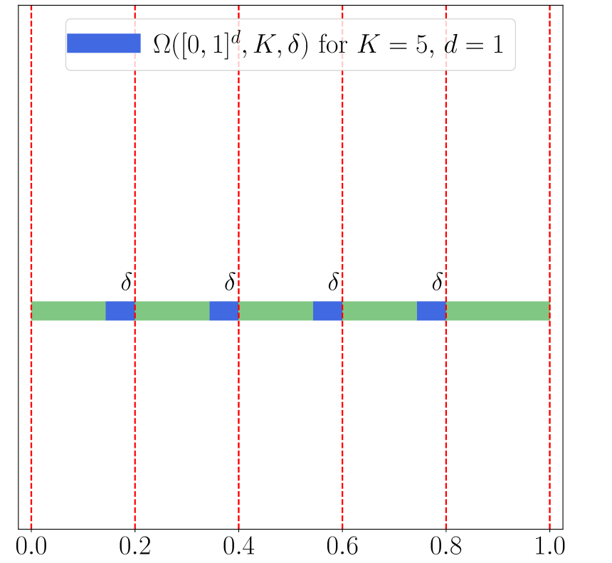
  (a)

  

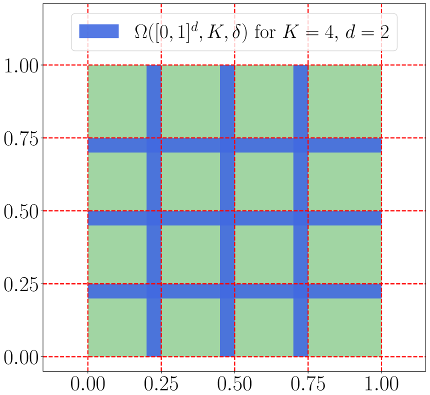
  (b)

  Figure 2: Two examples of trifling regions. (a) $K=5,d=1$. (b) $K=4,d=2$.

• Let ${\textnormal{H\"{o}lder}([0,1]^{d},\alpha,\lambda)}$ denote the space of Hölder continuous functions on $[0,1]^{d}$ of order $\alpha\in(0,1]$ with a Hölder constant $\lambda>0$.

• For a continuous piecewise linear function $f(x)$, the $x$ values where the slope changes are typically called breakpoints.

• Let $\textnormal{CPwL}(\mathbb{R},n)$ denote the space that consists of all continuous piecewise linear functions with at most $n$ breakpoints on $\mathbb{R}$.

• Let $\sigma:\mathbb{R}\to\mathbb{R}$ denote the rectified linear unit (ReLU), i.e. $\sigma(x)=\max\{0,x\}$. With a slight abuse of notation, we define $\sigma:\mathbb{R}^{d}\to\mathbb{R}^{d}$ as $\sigma({\bm{x}})=\left[\begin{array}[]{c}\max\{0,x_{1}\}\\ \vdots\\ \max\{0,x_{d}\}\end{array}\right]$ for any ${\bm{x}}=[x_{1},\cdots,x_{d}]^{T}\in\mathbb{R}^{d}$.

• We will use $\mathcal{NN}$ to denote a function implemented by a ReLU network for short and use Python-type notations to specify a class of functions implemented by ReLU networks with several conditions, e.g., $\mathcal{NN}(\textnormal{c}_{1};\ \textnormal{c}_{2};\ \cdots;\ \textnormal{c}_{m})$ is a set of functions implemented by ReLU networks satisfying $m$ conditions given by $\{\textnormal{c}_{i}\}_{1\leq i\leq m}$, each of which may specify the number of inputs (#input), the number of outputs (#output), the number of hidden layers (depth), the total number of parameters (#parameter), and the width in each hidden layer (width vec), the maximum width of all hidden layers (width), etc. For example, if $\phi\in\mathcal{NN}(\textnormal{\#input}=2;\ \textnormal{width\hskip 0.5ptvec}=[100,100];\ \textnormal{\#output}=1)$, then $\phi$ is a function satisfying

  • $\phi$ maps from $\mathbb{R}^{2}$ to $\mathbb{R}$.

  • $\phi$ can be implemented by a ReLU network with two hidden layers and the number of neurons in each hidden layer is $100$.

• For any function $\phi\in\mathcal{NN}(\textnormal{\#input}=d;\ \textnormal{width\hskip 0.5ptvec}=[N_{1},N_{2},\cdots,N_{L}];\ \textnormal{\#output}=1)$, if we set $N_{0}=d$ and $N_{L+1}=1$, then the architecture of the network implementing $\phi$ can be briefly described as follows:

  $$\bm{x}=\widetilde{\bm{h}}_{0}\mathop{\vbox{\hbox{\scalebox{1.0}[1.0]{ \leavevmode\hbox to45.04pt{\vbox to16.57pt{\text{[drawing]}}}}}}}^{\bm{W}_{0},\ \bm{b}_{0}}_{\mathcal{L}_{0}}\bm{h}_{1}\mathop{\vbox{\hbox{\scalebox{1.0}[1.0]{ \leavevmode\hbox to25.26pt{\vbox to0.72pt{\text{[drawing]}}}}}}}^{\sigma}\widetilde{\bm{h}}_{1}\ \cdots\ \mathop{\vbox{\hbox{\scalebox{1.0}[1.0]{ \leavevmode\hbox to53.73pt{\vbox to0.72pt{\text{[drawing]}}}}}}}^{\bm{W}_{L-1},\ \bm{b}_{L-1}}_{\mathcal{L}_{L-1}}\bm{h}_{L}\mathop{\vbox{\hbox{\scalebox{1.0}[1.0]{ \leavevmode\hbox to25.26pt{\vbox to0.72pt{\text{[drawing]}}}}}}}^{\sigma}\widetilde{\bm{h}}_{L}\mathop{\vbox{\hbox{\scalebox{1.0}[1.0]{ \leavevmode\hbox to43.91pt{\vbox to0.72pt{\text{[drawing]}}}}}}}^{\bm{W}_{L},\ \bm{b}_{L}}_{\mathcal{L}_{L}}\bm{h}_{L+1}=\phi(\bm{x}),$$

  where $\bm{W}_{i}\in\mathbb{R}^{N_{i+1}\times N_{i}}$ and $\bm{b}_{i}\in\mathbb{R}^{N_{i+1}}$ are the weight matrix and the bias vector in the $i$-th affine linear transformation $\mathcal{L}_{i}$, respectively, i.e.,

  $$\bm{h}_{i+1}=\bm{W}_{i}\cdot\widetilde{\bm{h}}_{i}+\bm{b}_{i}\eqqcolon\mathcal{L}_{i}(\widetilde{\bm{h}}_{i}),\quad\textnormal{for $i=0,1,\cdots,L$,}$$

  and

  $$\widetilde{\bm{h}}_{i}=\sigma(\bm{h}_{i}),\quad\textnormal{for $i=1,2,\cdots,L$.}$$

  In particular, $\phi$ can be represented in a form of function compositions as follows.

  $$\phi=\mathcal{L}_{L}\circ\sigma\circ\mathcal{L}_{L-1}\circ\sigma\circ\ \cdots\ \circ\sigma\circ\mathcal{L}_{1}\circ\sigma\circ\mathcal{L}_{0},$$

  which has been illustrated in Figure 3.

  

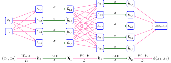
  Figure 3: An example of a ReLU network with width $5$ and depth $2$.

• The expression “a network with width $N$ and depth $L$” means

  • The maximum width of this network for all hidden layers is no more than $N$.

  • The number of hidden layers of this network is no more than $L$.

2.2 Proof of Theorem 1.1

The key point is to construct piecewise constant functions to approximate continuous functions in the proof. However, it is impossible to construct a piecewise constant function implemented by a ReLU network due to the continuity of ReLU networks. Thus, we introduce the trifling region $\Omega([0,1]^{d},K,\delta)$, defined in Equation (2.1), and use ReLU networks to implement piecewise constant functions outside the trifling region. To prove Theorem 1.1, we first introduce a weaker variant of Theorem 1.1, showing how to construct ReLU networks to pointwisely approximate continuous functions except for the trifling region.

Theorem 2.1.

Given a function $f\in C([0,1]^{d})$, for any $N\in\mathbb{N}^{+}$ and $L\in\mathbb{N}^{+}$, there exists a function $\phi$ implemented by a ReLU network with width $\max\big{\{}8d\lfloor N^{1/d}\rfloor+3d,\,16N+30\big{\}}$ and depth $11L+18$ such that $\|\phi\|_{L^{\infty}(\mathbb{R}^{d})}\leq|f({\bm{0}})|+\omega_{f}(\sqrt{d})$ and

$$|f({\bm{x}})-\phi({\bm{x}})|\leq 130\sqrt{d}\,\omega_{f}\Big{(}\big{(}N^{2}L^{2}\log_{3}(N+2)\big{)}^{-1/d}\Big{)},\quad\textnormal{for any ${\bm{x}}\in[0,1]^{d}\backslash\Omega([0,1]^{d},K,\delta)$},$$

where $K=\lfloor N^{1/d}\rfloor^{2}\lfloor L^{1/d}\rfloor^{2}\big{\lfloor}\lfloor\log_{3}(N+2)\rfloor^{1/d}\big{\rfloor}$ and $\delta$ is an arbitrary number in $(0,\tfrac{1}{3K}]$.

With Theorem 2.1 that will be proved in Section 3, we can easily prove Theorem 1.1 for the case $p\in[1,\infty)$. To attain the rate in $L^{\infty}$-norm, we need to control the approximation error in the trifling region. To this end, we introduce a theorem to deal with the approximation inside the trifling region $\Omega([0,1]^{d},K,\delta)$.

Theorem 2.2 (Theorem $3.7$ of [44] or Theorem $2.1$ of [24]).

Given any $\varepsilon>0$, $N,L,K\in\mathbb{N}^{+}$, and $\delta\in(0,\tfrac{1}{3K}]$, assume $f$ is a continuous function in $C([0,1]^{d})$ and ${\widetilde{\phi}}$ can be implemented by a ReLU network with width $N$ and depth $L$. If

$$|f({\bm{x}})-{\widetilde{\phi}}({\bm{x}})|\leq\varepsilon,\quad\textnormal{for any ${\bm{x}}\in[0,1]^{d}\backslash\Omega([0,1]^{d},K,\delta)$,}$$

then there exists a function $\phi$ implemented by a new ReLU network with width $3^{d}(N+4)$ and depth $L+2d$ such that

$$|f({\bm{x}})-\phi({\bm{x}})|\leq\varepsilon+d\cdot\omega_{f}(\delta),\quad\textnormal{for any ${\bm{x}}\in[0,1]^{d}$.}$$

Now we are ready to prove Theorem 1.1 by assuming Theorem 2.1 is true, which will be proved later in Section 3.

Proof of Theorem 1.1.

We may assume $f$ is not a constant function since it is a trivial case. Then $\omega_{f}(r)>0$ for any $r>0$. Let us first consider the case $p\in[1,\infty)$. Set $K=\lfloor N^{1/d}\rfloor^{2}\lfloor L^{1/d}\rfloor^{2}\big{\lfloor}\lfloor\log_{3}(N+2)\rfloor^{1/d}\big{\rfloor}$ and choose a small $\delta\in(0,\tfrac{1}{3K}]$ such that

$$\begin{split}Kd\delta\big{(}{\color[rgb]{0,0,0}2}|f({\bm{0}})|+{\color[rgb]{0,0,0}2}\omega_{f}(\sqrt{d})\big{)}^{p}&=\lfloor N^{1/d}\rfloor^{2}\lfloor L^{1/d}\rfloor^{2}\big{\lfloor}\lfloor\log_{3}(N+2)\rfloor^{1/d}\big{\rfloor}d\delta\big{(}2|f({\bm{0}})|+2\omega_{f}(\sqrt{d})\big{)}^{p}\\ &\leq\bigg{(}\omega_{f}\Big{(}\big{(}N^{2}L^{2}\log_{3}(N+2)\big{)}^{-1/d}\Big{)}\bigg{)}^{p}.\end{split}$$

By Theorem 2.1, there exists a function $\phi$ implemented by a ReLU network with width

$$\max\big{\{}8d\lfloor N^{1/d}\rfloor+3d,\,16N+30\big{\}}\leq 16\max\big{\{}d\lfloor N^{1/d}\rfloor,\,N+2\big{\}}$$

and depth $11L+18$ such that $\|\phi\|_{L^{\infty}(\mathbb{R}^{d})}\leq|f({\bm{0}})|+\omega_{f}(\sqrt{d})$ and

$$|f({\bm{x}})-\phi({\bm{x}})|\leq 130\sqrt{d}\,\omega_{f}\Big{(}\big{(}N^{2}L^{2}\log_{3}(N+2)\big{)}^{-1/d}\Big{)},\quad\textnormal{for any ${\bm{x}}\in[0,1]^{d}\backslash\Omega([0,1]^{d},K,\delta)$}.$$

It follows from $\mu(\Omega([0,1]^{d},K,\delta))\leq Kd\delta$ and $\|f\|_{L^{\infty}([0,1]^{d})}\leq|f({\bm{0}})|+\omega_{f}(\sqrt{d})$ that

$$\begin{split}\|f-\phi\|_{L^{p}([0,1]^{d})}^{p}&=\int_{\Omega([0,1]^{d},K,\delta)}|f({\bm{x}})-\phi({\bm{x}})|^{p}\textnormal{d}{\bm{x}}+\int_{[0,1]^{d}\backslash\Omega([0,1]^{d},K,\delta)}|f({\bm{x}})-\phi({\bm{x}})|^{p}\textnormal{d}{\bm{x}}\\ &\leq Kd\delta\big{(}{\color[rgb]{0,0,0}2}|f({\bm{0}})|+{\color[rgb]{0,0,0}2}\omega_{f}(\sqrt{d})\big{)}^{p}+\bigg{(}130\sqrt{d}\,\omega_{f}\Big{(}\big{(}N^{2}L^{2}\log_{3}(N+2)\big{)}^{-1/d}\Big{)}\bigg{)}^{p}\\ &\leq\bigg{(}\omega_{f}\Big{(}\big{(}N^{2}L^{2}\log_{3}(N+2)\big{)}^{-1/d}\Big{)}\bigg{)}^{p}+\bigg{(}130\sqrt{d}\,\omega_{f}\Big{(}\big{(}N^{2}L^{2}\log_{3}(N+2)\big{)}^{-1/d}\Big{)}\bigg{)}^{p}\\ &\leq\bigg{(}131\sqrt{d}\,\omega_{f}\Big{(}\big{(}N^{2}L^{2}\log_{3}(N+2)\big{)}^{-1/d}\Big{)}\bigg{)}^{p}.\end{split}$$

Hence, $\|f-\phi\|_{L^{p}([0,1]^{d})}\leq 131\sqrt{d}\,\omega_{f}\Big{(}\big{(}N^{2}L^{2}\log_{3}(N+2)\big{)}^{-1/d}\Big{)}$.

Next, let us discuss the case $p=\infty$. Set $K=\lfloor N^{1/d}\rfloor^{2}\lfloor L^{1/d}\rfloor^{2}\big{\lfloor}\lfloor\log_{3}(N+2)\rfloor^{1/d}\big{\rfloor}$ and choose a small $\delta\in(0,\tfrac{1}{3K}]$ such that

$$d\cdot\omega_{f}(\delta)\leq\omega_{f}\Big{(}\big{(}N^{2}L^{2}\log_{3}(N+2)\big{)}^{-1/d}\Big{)}.$$

By Theorem 2.1, there exists a function ${\widetilde{\phi}}$ implemented by a ReLU network with width $\max\big{\{}8d\lfloor N^{1/d}\rfloor+3d,\,16N+30\big{\}}$ and depth $11L+18$ such that

$$|f({\bm{x}})-{\widetilde{\phi}}({\bm{x}})|\leq 130\sqrt{d}\,\omega_{f}\Big{(}\big{(}N^{2}L^{2}\log_{3}(N+2)\big{)}^{-1/d}\Big{)}\eqqcolon\varepsilon,$$

for any ${\bm{x}}\in[0,1]^{d}\backslash\Omega([0,1]^{d},K,\delta)$. By Theorem 2.2, there exists a function $\phi$ implemented by a ReLU network with width

$$3^{d}\Big{(}\max\big{\{}8d\lfloor N^{1/d}\rfloor+3d,\,16N+30\big{\}}+4\Big{)}\leq 3^{d+3}\max\big{\{}d\lfloor N^{1/d}\rfloor,\,N+2\big{\}}$$

and depth $11L+18+2d$ such that

$$|f({\bm{x}})-\phi({\bm{x}})|\leq\varepsilon+d\cdot\omega_{f}(\delta)\leq 131\sqrt{d}\,\omega_{f}\Big{(}\big{(}N^{2}L^{2}\log_{3}(N+2)\big{)}^{-1/d}\Big{)},\quad\textnormal{for any ${\bm{x}}\in[0,1]^{d}$}.$$

So we finish the proof. ∎

2.3 Optimality

This section will show that the approximation rates in Theorem 1.1 and Corollary 1.3 are optimal and there is no room to improve for the function class ${\textnormal{H\"{o}lder}([0,1]^{d},\alpha,\lambda)}$. Therefore, the approximation rate for the whole continuous functions space in terms of width and depth in Theorem 1.1 cannot be improved. A typical method to characterize the optimal approximation theory of neural networks is to study the connection between the approximation error and Vapnik–Chervonenkis (VC) dimension [40, 41, 24, 44, 33]. This method relies on the VC-dimension upper bound given in [13]. In this paper, we adopt this method with several modifications to simplify the proof.

Let us first present the definitions of VC-dimension and related concepts. Let $H$ be a class of functions mapping from a general domain $\mathcal{X}$ to $\{0,1\}$. We say $H$ shatters the set $\{{\bm{x}}_{1},{\bm{x}}_{2},\cdots,{\bm{x}}_{m}\}\subseteq\mathcal{X}$ if

$$\Big{|}\Big{\{}\big{[}h({\bm{x}}_{1}),h({\bm{x}}_{2}),\cdots,h({\bm{x}}_{m})\big{]}^{T}\in\{0,1\}^{m}:h\in H\Big{\}}\Big{|}=2^{m},$$

where $|\cdot|$ denotes the size of a set. This equation means, given any $\theta_{i}\in\{0,1\}$ for $i=1,2,\cdots,m$, there exists $h\in H$ such that $h({\bm{x}}_{i})=\theta_{i}$ for all $i$. For a general function set ${\mathscr{F}}$ mapping from $\mathcal{X}$ to $\mathbb{R}$, we say ${\mathscr{F}}$ shatters $\{{\bm{x}}_{1},{\bm{x}}_{2},\cdots,{\bm{x}}_{m}\}\subseteq\mathcal{X}$ if $\mathcal{T}\circ{\mathscr{F}}$ does, where

$$\mathcal{T}(t)\coloneqq\left\{\begin{array}[]{ll}1,&\ t\geq 0,\\ 0,&\ t<0\phantom{,}\end{array}\right.\quad\textnormal{and}\quad\mathcal{T}\circ{\mathscr{F}}\coloneqq\{\mathcal{T}\circ f:f\in{\mathscr{F}}\}.$$

For any $m\in\mathbb{N}^{+}$, we define the growth function of $H$ as

$$\Pi_{H}(m)\coloneqq\max_{{\bm{x}}_{1},{\bm{x}}_{2},\cdots,{\bm{x}}_{m}\in\mathcal{X}}\Big{|}\Big{\{}\big{[}h({\bm{x}}_{1}),h({\bm{x}}_{2}),\cdots,h({\bm{x}}_{m})\big{]}^{T}\in\{0,1\}^{m}:h\in H\Big{\}}\Big{|}.$$

Definition 2.3 (VC-dimension).

Let $H$ be a class of functions from $\mathcal{X}$ to $\{0,1\}$. The VC-dimension of $H$, denoted by $\textnormal{VCDim}(H)$, is the size of the largest shattered set, namely,

$$\textnormal{VCDim}(H)\coloneqq\sup\{m\in\mathbb{N}^{+}:\Pi_{H}(m)=2^{m}\}$$

if $\{m\in\mathbb{N}^{+}:\Pi_{H}(m)=2^{m}\}$ is not empty. In the case of $\{m\in\mathbb{N}^{+}:\Pi_{H}(m)=2^{m}\}=\emptyset$, we may define $\textnormal{VCDim}(H)=0$.

Let ${\mathscr{F}}$ be a class of functions from $\mathcal{X}$ to $\mathbb{R}$. The VC-dimension of ${\mathscr{F}}$, denoted by $\textnormal{VCDim}({\mathscr{F}})$, is defined by $\textnormal{VCDim}({\mathscr{F}})\coloneqq\textnormal{VCDim}(\mathcal{T}\circ{\mathscr{F}})$, where

$$\mathcal{T}(t)\coloneqq\left\{\begin{array}[]{ll}1,&\ t\geq 0,\\ 0,&\ t<0\phantom{,}\end{array}\right.\quad\textnormal{and}\quad\mathcal{T}\circ{\mathscr{F}}\coloneqq\{\mathcal{T}\circ f:f\in{\mathscr{F}}\}.$$

In particular, the expression “VC-dimension of a network (architecture)” means the VC-dimension of the function set that consists of all functions implemented by this network (architecture).

We remark that one may also define $\textnormal{VCDim}({\mathscr{F}})$ as $\textnormal{VCDim}({\mathscr{F}})\coloneqq\textnormal{VCDim}(\widetilde{\mathcal{T}}\circ{\mathscr{F}})$, where

$$\widetilde{\mathcal{T}}(t)\coloneqq\left\{\begin{array}[]{ll}1,&\ t>0,\\ 0,&\ t\leq 0\phantom{,}\end{array}\right.\quad\textnormal{and}\quad\widetilde{\mathcal{T}}\circ{\mathscr{F}}\coloneqq\{\widetilde{\mathcal{T}}\circ f:f\in{\mathscr{F}}\}.$$

Note that function spaces generated by networks are closed under linear transformation. Thus, these two definitions of VC-dimension are equivalent.

The theorem below, similar to Theorem $4.17$ of [44], reveals the connection between VC-dimension and the approximation rate.

Theorem 2.4.

Assume ${\mathscr{F}}$ is a set of functions mapping from $[0,1]^{d}$ to $\mathbb{R}$. For any $\varepsilon>0$, if $\textnormal{VCDim}({\mathscr{F}})\geq 1$ and

$$\inf_{\phi\in{\mathscr{F}}}\|\phi-f\|_{L^{\infty}([0,1]^{d})}\leq\varepsilon,\quad\textnormal{for any $f\in\textnormal{H\"{o}lder}([0,1]^{d},\alpha,1)$,}$$ (2.2)

then $\textnormal{VCDim}({\mathscr{F}})\geq(9\varepsilon)^{-d/\alpha}$.

This theorem demonstrates the connection between VC-dimension of ${\mathscr{F}}$ and the approximation rate using elements of ${\mathscr{F}}$ to approximate functions in $\textnormal{H\"{o}lder}([0,1]^{d},\alpha,\lambda)$. To be precise, the VC-dimension of ${\mathscr{F}}$ determines an approximation rate lower bound $\textnormal{VCDim}({\mathscr{F}})^{-\alpha/d}/9$, which is the best possible approximation rate. Denote the best approximation error of functions in $\textnormal{H\"{o}lder}([0,1]^{d},\alpha,1)$ approximated by ReLU networks with width $N$ and depth $L$ as

$$\mathcal{E}_{\alpha,d}(N,L)\coloneqq\sup_{f\in\textnormal{H\"{o}lder}([0,1]^{d},\alpha,1)}\bigg{(}\inf_{\phi\in\mathcal{NN}(\textnormal{width}\leq N;\,\textnormal{depth}\leq L)}\|\phi-f\|_{L^{\infty}([0,1]^{d})}\bigg{)}.$$

We have three remarks listed below.

1. A large VC-dimension cannot guarantee a good approximation rate. For example, it is easy to verify that

   $$\textnormal{VCDim}\Big{(}\big{\{}f:f(x)=\cos(ax),\ a\in\mathbb{R}\big{\}}\Big{)}=\infty.$$

   However, functions in $\big{\{}f:f(x)=\cos(ax),\ a\in\mathbb{R}\big{\}}$ cannot approximate Hölder continuous functions well.

2. A large VC-dimension is necessary for a good approximation rate, because the best possible approximation rate is controlled by an expression of VC-dimension, as shown in Theorem 2.4. It is shown in Theorem $6$ and $8$ of [13] that the VC-dimension of ReLU networks has two types of upper bounds: ${\mathcal{O}}(WL\ln W)$ and ${\mathcal{O}}(WU)$. Here, $W$, $L$, and $U$ are the numbers of parameters, layers, and neurons, respectively. If we let $N$ denote the maximum width of the network, then $W={\mathcal{O}}(N^{2}L)$ and $U={\mathcal{O}}(NL)$, implying that

   $$WL\ln W={\mathcal{O}}\big{(}N^{2}L\cdot L\ln(N^{2}L)\big{)}={\mathcal{O}}\big{(}N^{2}L^{2}\ln(NL)\big{)}$$

   and

   $$WU={\mathcal{O}}(N^{2}L\cdot NL)={\mathcal{O}}(N^{3}L^{2}).$$

   It follows that

   $$\textnormal{VCDim}\big{(}\mathcal{NN}(\textnormal{width}\leq N;\ \textnormal{depth}\leq L)\big{)}\leq\min\Big{\{}{\mathcal{O}}\big{(}N^{2}L^{2}\ln(NL)\big{)},{\mathcal{O}}(N^{3}L^{2})\Big{\}},$$

   deducing

   where $C_{1}(\alpha,d)$ and $C_{2}(\alpha,d)$ are two positive constants determined by $s,d$, and $C_{2}(s,d)$ can be explicitly expressed.

   • When $L=L_{0}$ is fixed, Equation (2.3) implies

     $$C_{1}(\alpha,d,L_{0})(N^{2}\ln N)^{-\alpha/d}\,\leq\,\mathcal{E}_{\alpha,d}(N,L_{0})\,\leq\,C_{2}(\alpha,d,L_{0})(N^{2}\ln N)^{-\alpha/d},$$

     where $C_{1}(\alpha,d,L_{0})$ and $C_{2}(\alpha,d,L_{0})$ are two positive constants determined by $\alpha,d,L_{0}$.

   • When $N=N_{0}$ is fixed, Equation (2.3) implies

     $$C_{1}(\alpha,d,N_{0})L^{-2\alpha/d}\,\leq\,\mathcal{E}_{\alpha,d}(N_{0},L)\,\leq\,C_{2}(\alpha,d,N_{0})L^{-2\alpha/d},$$

     where $C_{1}(\alpha,d,N_{0})$ and $C_{2}(\alpha,d,N_{0})$ are two positive constants determined by $\alpha,d,N_{0}$.

   • It is easy to verify that Equation (2.3) is tight except for the following region

     $$\big{\{}(N,L)\in\mathbb{N}^{2}:C_{3}(\alpha,d)\leq N\leq L^{C_{4}(\alpha,d)}\big{\}},$$

     $C_{3}=C_{3}(\alpha,d)$ and $C_{4}=C_{4}(\alpha,d)$ are two positive constants. See Figure 1 for an illustration for the case $C_{3}=1000$ and $C_{4}=1/100$.

Finally, let us present the detailed proof of Theorem 2.4.

Proof of Theorem 2.4.

Recall that the VC-dimension of a function set is defined as the size of the largest set of points that this class of functions can shatter. So our goal is to find a subset of ${\mathscr{F}}$ to shatter ${\mathcal{O}}(\varepsilon^{-d/\alpha})$ points in $[0,1]^{d}$, which can be divided into two steps.

• Construct $\{f_{\chi}:\chi\in\mathscr{B}\}\subseteq\textnormal{H\"{o}lder}([0,1]^{d},\alpha,1)$ that scatters ${\mathcal{O}}(\varepsilon^{-d/\alpha})$ points, where ${\mathscr{B}}$ is a set defined later.

• Design $\phi_{\chi}\in{\mathscr{F}}$, for each $\chi\in{\mathscr{B}}$, based on $f_{\chi}$ and Equation (2.2) such that $\{\phi_{\chi}:\chi\in{\mathscr{F}}\}\subseteq{\mathscr{F}}$ also shatters ${\mathcal{O}}(\varepsilon^{-d/\alpha})$ points.

The details of these two steps can be found below.

Step $1\colon$ Construct $\{f_{\chi}:\chi\in\mathscr{B}\}\subseteq\textnormal{H\"{o}lder}([0,1]^{d},\alpha,1)$ that scatters ${\mathcal{O}}(\varepsilon^{-d/\alpha})$ points.

We may assume $\varepsilon\leq 2/9$ since the case $\varepsilon>2/9$ is trivial. In fact, $\varepsilon>2/9$ implies

$$\textnormal{VCDim}({\mathscr{F}})\geq 1\geq 1/2\geq 2^{-d/\alpha}>(9\varepsilon)^{-d/\alpha}.$$

Let $K=\lfloor\left(9\varepsilon/2\right)^{-1/\alpha}\rfloor\in\mathbb{N}^{+}$ and divide $[0,1]^{d}$ into $K^{d}$ non-overlapping sub-cubes $\{Q_{{\bm{\beta}}}\}_{{\bm{\beta}}}$ as follows:

$$Q_{{\bm{\beta}}}\coloneqq\big{\{}{\bm{x}}=[x_{1},x_{2},\cdots,x_{d}]^{T}\in[0,1]^{d}:x_{i}\in[\tfrac{\beta_{i}}{K},\tfrac{\beta_{i}+1}{K}],\ i=1,2,\cdots,d\big{\}},$$

for any index vector ${{\bm{\beta}}}=[\beta_{1},\beta_{2},\cdots,\beta_{d}]^{T}\in\{0,1,\cdots,K-1\}^{d}$.

Let $Q(\bm{x}_{0},\eta)$ denote the closed cube with center ${\bm{x}}_{0}\in\mathbb{R}^{d}$ and sidelength $\eta>0$. Define a function $\zeta_{Q}$ on $[0,1]^{d}$ corresponding to $Q=Q(\bm{x}_{0},\eta)\subseteq[0,1]^{d}$ such that:

• $\zeta_{Q}(\bm{x}_{0})=(\eta/2)^{\alpha}/2$;

• $\zeta_{Q}(\bm{x})=0$ for any ${\bm{x}}\notin Q\backslash\partial Q$, where $\partial Q$ is the boundary of $Q$;

• $\zeta_{Q}$ is linear on the line that connects ${\bm{x}}_{0}$ and ${\bm{x}}$ for any ${\bm{x}}\in\partial Q$.

Define

$$\mathscr{B}\coloneqq\big{\{}\chi:\chi\textnormal{ is a map from }\{0,1,\cdots,K-1\}^{d}\textnormal{ to }\{-1,1\}\big{\}}.$$

For each $\chi\in\mathscr{B}$, we define

$$f_{\chi}(\bm{x})\coloneqq\sum_{{{\bm{\beta}}}\in\{0,1,\cdots,K-1\}^{d}}\chi({{\bm{\beta}}})\zeta_{Q_{{\bm{\beta}}}}(\bm{x}),$$

where $\zeta_{Q_{{\bm{\beta}}}}(\bm{x})$ is the associated function introduced just above. It is easy to check that $\{f_{\chi}:\chi\in\mathscr{B}\}\subseteq\textnormal{H\"{o}lder}([0,1]^{d},\alpha,1)$ can shatter $K^{d}={\mathcal{O}}(\varepsilon^{-d/\alpha})$ points in $[0,1]^{d}$.

Step $2\colon$ Construct $\{\phi_{\chi}:\chi\in\mathscr{B}\}$ that also scatters ${\mathcal{O}}(\varepsilon^{-d/\alpha})$ points.

By Equation (2.2), for each $\chi\in{\mathscr{B}}$, there exists $\phi_{\chi}\in{\mathscr{F}}$ such that

$$\|\phi_{\chi}-f_{\chi}\|_{L^{\infty}([0,1]^{d})}\leq\varepsilon+\varepsilon/81.$$

Let $\mu(\cdot)$ denote the Lebesgue measure of a set. Then, for each $\chi\in{\mathscr{B}}$, there exists ${\mathcal{H}}_{\chi}\subseteq[0,1]^{d}$ with $\mu({\mathcal{H}}_{\chi})=0$ such that

$$|\phi_{\chi}({\bm{x}})-f_{\chi}({\bm{x}})|\leq\tfrac{82}{81}\varepsilon,\quad\textnormal{for any ${\bm{x}}\in[0,1]\backslash{\mathcal{H}}_{\chi}$}.$$

Set ${\mathcal{H}}=\cup_{\chi\in{\mathscr{B}}}{\mathcal{H}}_{\chi}$, then we have $\mu({\mathcal{H}})=0$ and

$$|\phi_{\chi}({\bm{x}})-f_{\chi}({\bm{x}})|\leq\tfrac{82}{81}\varepsilon,\quad\textnormal{for any $\chi\in{\mathscr{B}}$ and ${\bm{x}}\in[0,1]\backslash{\mathcal{H}}$}.$$ (2.4)

Since $Q_{{\bm{\beta}}}$ has a sidelength $\tfrac{1}{K}=\tfrac{1}{\lfloor(9\varepsilon/2)^{-1/\alpha}\rfloor}$, we have, for each ${{\bm{\beta}}}\in\{0,1,\cdots,K-1\}^{d}$ and any $\bm{x}\in\tfrac{1}{10}Q_{{\bm{\beta}}}$,

$$|f_{\chi}(\bm{x})|=|\zeta_{Q_{{\bm{\beta}}}}(\bm{x})|\geq\tfrac{9}{10}|\zeta_{Q_{{\bm{\beta}}}}(\bm{x}_{Q_{{\bm{\beta}}}})|=\tfrac{9}{10}(\tfrac{1}{2\lfloor(9\varepsilon/2)^{-1/\alpha}\rfloor})^{\alpha}/2\geq\tfrac{81}{80}\varepsilon,$$ (2.5)

where $\bm{x}_{Q_{{\bm{\beta}}}}$ is the center of $Q_{{\bm{\beta}}}$.

Note that $(\tfrac{1}{10}Q_{\bm{\beta}})\backslash{\mathcal{H}}$ is not empty, since $\mu\big{(}(\tfrac{1}{10}Q_{\bm{\beta}})\backslash{\mathcal{H}}\big{)}>0$ for each ${\bm{\beta}}\in\{0,1,\cdots,K-1\}^{d}$. Together with Equations (2.4) and (2.5), there exists ${\bm{x}}_{\bm{\beta}}\in(\tfrac{1}{10}Q_{\bm{\beta}})\backslash{\mathcal{H}}$ such that, for each ${\bm{\beta}}\in\{0,1,\cdots,K-1\}^{d}$ and each $\chi\in{\mathscr{B}}$,

$$|f_{\chi}({\bm{x}}_{{\bm{\beta}}})|\geq\tfrac{81}{80}\varepsilon>\tfrac{82}{81}\varepsilon\geq|f_{\chi}({\bm{x}}_{{\bm{\beta}}})-\phi_{\chi}({\bm{x}}_{{\bm{\beta}}})|.$$

Hence, $f_{\chi}({\bm{x}}_{{\bm{\beta}}})$ and $\phi_{\chi}({\bm{x}}_{{\bm{\beta}}})$ have the same sign for each $\chi\in\mathscr{B}$ and ${{\bm{\beta}}}\in\{0,1,\cdots,K-1\}^{d}$. Then $\{\phi_{\chi}:\chi\in\mathscr{B}\}$ shatters $\big{\{}{\bm{x}}_{\bm{\beta}}:{\bm{\beta}}\in\{0,1,\cdots,K-1\}^{d}\big{\}}$ since $\{f_{\chi}:\chi\in\mathscr{B}\}$ shatters $\big{\{}{\bm{x}}_{\bm{\beta}}:{\bm{\beta}}\in\{0,1,\cdots,K-1\}^{d}\big{\}}$. Therefore,

$$\textnormal{VCDim}({\mathscr{F}})\geq\textnormal{VCDim}\big{(}\{\phi_{\chi}:\chi\in\mathscr{B}\}\big{)}\geq K^{d}=\lfloor(9\varepsilon/2)^{-1/\alpha}\rfloor^{d}\geq(9\varepsilon)^{-d/\alpha},$$

where the last inequality comes from the fact $\lfloor x\rfloor\geq x/2\geq x/(2^{1/\alpha})$ for any $x\in[1,\infty)$ and $\alpha\in(0,1]$. So we finish the proof. ∎

2.4 Approximation in irregular domain

We extend our analysis to general continuous functions defined on any irregular bounded set in $\mathbb{R}^{d}$. The key idea is to extend the target function to a hypercube while preserving the modulus of continuity. The extension of continuous (smooth) functions has been widely studied, e.g., [39] for smooth functions and [38] for continuous functions. For simplicity, we use Lemma $4.2$ of [33]. The proof can be found therein. For a general set $E\subseteq\mathbb{R}^{d}$, the modulus of continuity of $f\in C(E)$ is defined via

$$\omega_{f}^{E}(r)\coloneqq\sup\big{\{}|f(\bm{x})-f(\bm{y})|:\bm{x},\bm{y}\in E,\ \|\bm{x}-\bm{y}\|_{2}\leq r\big{\}},\quad\textnormal{for any $r\geq 0$}.$$

In particular, $\omega_{f}(\cdot)$ is short of $\omega_{f}^{E}(\cdot)$ in the case of $E=[0,1]^{d}$. Then, Theorem 1.1 can be generalized to $f\in C(E)$ for any bounded set $E\subseteq[-R,R]^{d}$ with $R>0$, as shown in the following theorem.

Theorem 2.5.

Given any bounded continuous function $f\in C(E)$ with $E\subseteq[-R,R]^{d}$ and $R>0$, for any $N\in\mathbb{N}^{+}$, $L\in\mathbb{N}^{+}$, and $p\in[1,\infty]$, there exists a function $\phi$ implemented by a ReLU network with width $C_{1}\max\big{\{}d\lfloor N^{1/d}\rfloor,\,N+2\big{\}}$ and depth $11L+C_{2}$ such that

$$\|f-\phi\|_{L^{p}(E)}\leq 131(2R)^{d/p}\sqrt{d}\,\omega_{f}^{E}\Big{(}2R\big{(}N^{2}L^{2}\log_{3}(N+2)\big{)}^{-1/d}\Big{)},$$

where $C_{1}=16$ and $C_{2}=18$ if $p\in[1,\infty)$; $C_{1}=3^{d+3}$ and $C_{2}=18+2d$ if $p=\infty$.

Proof.

Given any bounded continuous function $f\in C(E)$, by Lemma $4.2$ of [33] via setting $S=[-R,R]^{d}$, there exists $g\in C([-R,R]^{d})$ such that

• $g({\bm{x}})=f({\bm{x}})$ for any ${\bm{x}}\in E\subseteq S=[-R,R]^{d}$;

• $\omega_{g}^{S}(r)=\omega_{f}^{E}(r)$ for any $r\geq 0$.

Define

$${\widetilde{g}}({\bm{x}})\coloneqq g(2R{\bm{x}}-R),\quad\textnormal{for any ${\bm{x}}\in[0,1]^{d}$.}$$

By applying Theorem 1.1 to ${\widetilde{g}}\in C([0,1]^{d})$, there exists a function ${\widetilde{\phi}}$ implemented by a ReLU network with width $C_{1}\max\big{\{}d\lfloor N^{1/d}\rfloor,\,N+2\big{\}}$ and depth $11L+C_{2}$ such that

$$\|{\widetilde{\phi}}-{\widetilde{g}}\|_{L^{p}([0,1]^{d})}\leq 131\sqrt{d}\,\omega_{\widetilde{g}}\Big{(}\big{(}N^{2}L^{2}\log_{3}(N+2)\big{)}^{-1/d}\Big{)},$$

where $C_{1}=16$ and $C_{2}=18$ if $p\in[1,\infty)$; $C_{1}=3^{d+3}$ and $C_{2}=18+2d$ if $p=\infty$.

Note that $f({\bm{x}})=g({\bm{x}})={\widetilde{g}}(\tfrac{{\bm{x}}+R}{2R})$ for any ${\bm{x}}\in E\subseteq S=[-R,R]^{d}$ and

$$\omega_{\widetilde{g}}(r)=\omega_{g}^{S}(2Rr)=\omega_{f}^{E}(2Rr),\quad\textnormal{ for any $r\geq 0$}.$$

Define $\phi({\bm{x}})\coloneqq{\widetilde{\phi}}(\tfrac{{\bm{x}}+R}{2R})={\widetilde{\phi}}\circ\mathcal{L}({\bm{x}})$ for any ${\bm{x}}\in\mathbb{R}^{d}$, where $\mathcal{L}:\mathbb{R}^{d}\to\mathbb{R}^{d}$ is an affine linear map given by $\mathcal{L}({\bm{x}})=\tfrac{{\bm{x}}+R}{2R}$. Clearly, $\phi$ can be implemented by a ReLU network with width $C_{1}\max\big{\{}d\lfloor N^{1/d}\rfloor,\,N+2\big{\}}$ and depth $11L+C_{2}$, where $C_{1}=16$ and $C_{2}=18$ if $p\in[1,\infty)$; $C_{1}=3^{d+3}$ and $C_{2}=18+2d$ if $p=\infty$. Moreover, for any ${\bm{x}}\in E\subseteq S=[-R,R]^{d}$, we have $\tfrac{{\bm{x}}+R}{2R}\in[0,1]^{d}$, implying

$$\begin{split}\|\phi-f\|_{L^{p}(E)}&=\|\phi-g\|_{L^{p}(E)}=\|{\widetilde{\phi}}\circ\mathcal{L}-{\widetilde{g}}\circ\mathcal{L}\|_{L^{p}(E)}\\ &\leq\|{\widetilde{\phi}}\circ\mathcal{L}-{\widetilde{g}}\circ\mathcal{L}\|_{L^{p}([-R,R]^{d})}=(2R)^{d/p}\|{\widetilde{\phi}}-{\widetilde{g}}\|_{L^{p}([0,1]^{d})}\\ &\leq 131(2R)^{d/p}\sqrt{d}\,\omega_{\widetilde{g}}\Big{(}\big{(}N^{2}L^{2}\log_{3}(N+2)\big{)}^{-1/d}\Big{)}\\ &=131(2R)^{d/p}\sqrt{d}\,\omega_{f}^{E}\Big{(}2R\big{(}N^{2}L^{2}\log_{3}(N+2)\big{)}^{-1/d}\Big{)}.\end{split}$$

With the discussion above, we have proved Theorem 2.5. ∎

3 Proof of Theorem 2.1

We will prove Theorem 2.1 in this section. We first present the key ideas in Section 3.1. The detailed proof is presented in Section 3.3, based on two propositions in Section 3.1, the proofs of which can be found in Section 4.

3.1 Key ideas of proving Theorem 2.1

Given an arbitrary $f\in C([0,1]^{d})$, our goal is to construct an almost piecewise constant function $\phi$ implemented by a ReLU network to approximate $f$ well. To this end, we introduce a piecewise constant function $f_{p}\approx f$ serving as an intermediate approximant in our construction in the sense that

$$f\approx f_{p}\textnormal{ on $[0,1]^{d}$}\quad\textnormal{and}\quad f_{p}\approx\phi\textnormal{ on $[0,1]^{d}\backslash\Omega([0,1]^{d},K,\delta)$}.$$

The approximation in $f\approx f_{p}$ is a simple and standard technique in constructive approximation. The most technical part is to design a ReLU network with the desired width and depth to implement a function $\phi$ with $\phi\approx f_{p}$ outside $\Omega([0,1]^{d},K,\delta)$. See Figure 4 for an illustration. The introduction of the trifling region is to ease the construction of $\phi$, which is a continuous piecewise linear function, to approximate the discontinuous function $f_{p}$ by removing the difficulty near discontinuous points, essentially smoothing $f_{p}$ by restricting the approximation domain in $[0,1]^{d}\backslash\Omega([0,1]^{d},K,\delta)$.

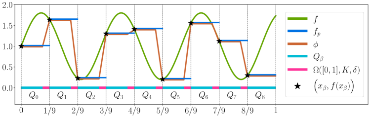
Figure 4: An illustration of $f$, $f_{p}$, $\phi$, $x_{\beta}$, $Q_{\beta}$, and the trifling region $\Omega([0,1]^{d},K,\delta)$ in the one-dimensional case for $\beta\in\{0,1,\cdots,K-1\}^{d}$, where $K=N^{2}L^{2}\lfloor\log_{3}(N+2)\rfloor$ and $d=1$ with $N=1$ and $L=3$. $f$ is the target function; $f_{p}$ is the piecewise constant function approximating $f$; $\phi$ is a function, implemented by a ReLU network, approximating $f$; and $x_{\beta}$ is a representative of $Q_{\beta}$. The measure of $\Omega([0,1]^{d},K,\delta)$ can be arbitrarily small as we shall see in the proof of Theorem 1.1.

Now let us discuss the detailed steps of construction.

1. First, divide $[0,1]^{d}$ into a union of important regions $\{Q_{\bm{\beta}}\}_{\bm{\beta}}$ and the trifling region $\Omega([0,1]^{d},K,\delta)$, where each $Q_{\bm{\beta}}$ is associated with a representative $\bm{x}_{\bm{\beta}}\in Q_{\bm{\beta}}$ such that $f_{p}(\bm{x}_{\bm{\beta}})=f(\bm{x}_{\bm{\beta}})$ for each index vector ${\bm{\beta}}\in\{0,1,\cdots,K-1\}^{d}$, where $K={\mathcal{O}}((N^{2}L^{2}\ln N)^{1/d})$ is the partition number per dimension (see Figure 7 for examples for $d=1$ and $d=2$).

2. Next, we design a vector function ${\bm{\Phi}}_{1}({\bm{x}})$ constructed via

   $${\bm{\Phi}}_{1}({\bm{x}})=\big{[}\phi_{1}(x_{1}),\,\phi_{1}(x_{2}),\,\cdots,\,\phi_{1}(x_{d})\big{]}^{T}$$

   to project the whole cube $Q_{\bm{\beta}}$ to a $d$-dimensional index ${\bm{\beta}}$ for each ${\bm{\beta}}$, where each one-dimensional function $\phi_{1}$ is a step function implemented by a ReLU network.

3. The third step is to solve a point fitting problem. To be precise, we construct a function $\phi_{2}$ implemented by a ReLU network to map ${\bm{\beta}}\in\{0,1,\cdots,K-1\}^{d}$ approximately to $f_{p}({\bm{x}}_{\bm{\beta}})=f({\bm{x}}_{\bm{\beta}})$. Then $\phi_{2}\circ{\bm{\Phi}}_{1}({\bm{x}})=\phi_{2}({\bm{\beta}})\approx f_{p}({\bm{x}}_{\bm{\beta}})=f({\bm{x}}_{\bm{\beta}})\approx f({\bm{x}})$ for any ${\bm{x}}\in Q_{\bm{\beta}}$ and each ${\bm{\beta}}$, implying $\phi\coloneqq\phi_{2}\circ{\bm{\Phi}}_{1}\approx f_{p}\approx f$ on $[0,1]^{d}\backslash\Omega([0,1]^{d},K,\delta)$. We would like to point out that we only need to care about the values of $\phi_{2}$ at a set of points $\{0,1,\cdots,K-1\}^{d}$ in the construction of $\phi_{2}$ according to our design $\phi=\phi_{2}\circ{\bm{\Phi}}_{1}$ as illustrated in Figure 5. Therefore, it is not necessary to care about the values of $\phi_{2}$ sampled outside the set $\{0,1,\cdots,K-1\}^{d}$, which is a key point to ease the design of a ReLU network to implement $\phi_{2}$ as we shall see later.

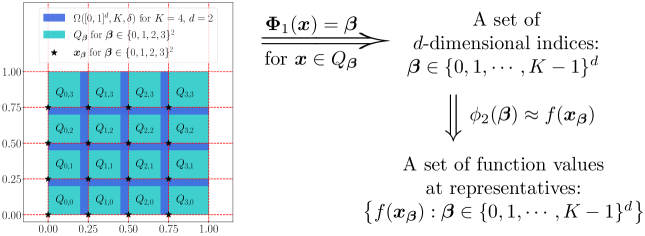
Figure 5: An illustration of the desired function $\phi=\phi_{2}\circ{\bm{\Phi}}_{1}$. Note that $\phi\approx f$ on $[0,1]^{d}\backslash\Omega([0,1]^{d},K,\delta)$, since $\phi({\bm{x}})=\phi_{2}\circ{\bm{\Phi}}_{1}({\bm{x}})=\phi_{2}({\bm{\beta}})\approx f({\bm{x}}_{\bm{\beta}})\approx f({\bm{x}})$ for any ${\bm{x}}\in Q_{\bm{\beta}}$ and each ${\bm{\beta}}\in\{0,1,\cdots,K-1\}^{d}$.

We remark that in Figure 5, we have

$$\phi({\bm{x}})=\phi_{2}\circ{\bm{\Phi}}_{1}({\bm{x}})=\phi_{2}({\bm{\beta}})\mathop{\approx}\limits^{{\mathscr{E}}_{1}}f({\bm{x}}_{\bm{\beta}})\mathop{\approx}\limits^{{\mathscr{E}}_{2}}f({\bm{x}})$$

for any ${\bm{x}}\in Q_{\bm{\beta}}$ and each ${\bm{\beta}}\in\{0,1,\cdots,K-1\}^{d}$. Thus, $\phi-f$ is bounded by ${\mathscr{E}}_{1}+{\mathscr{E}}_{2}$ outside the trifling region. Observe that ${\mathscr{E}}_{2}$ is bounded by $\omega_{f}(\sqrt{d}/K)$. As we shall see later in Section 3.3, ${\mathscr{E}}_{1}$ can also be bounded by $\omega_{f}(\sqrt{d}/K)$ by applying Proposition 3.2. Hence, $\phi-f$ is controlled by $2\omega_{f}(\sqrt{d}/K)$ outside the trifling region, which deduces the desired approximation error.

Finally, we discuss how to implement ${\bm{\Phi}}_{1}$ and $\phi_{2}$ by deep ReLU networks with width ${\mathcal{O}}(N)$ and depth ${\mathcal{O}}(L)$ using two propositions as we shall prove in Sections 4.2 and 4.3 later. We first show how to construct a ReLU network with the desired width and depth by Proposition 3.1 to implement a one-dimensional step function $\phi_{1}$. Then ${\bm{\Phi}}_{1}$ can be attained via defining

$${\bm{\Phi}}_{1}({\bm{x}})\coloneqq\big{[}\phi_{1}(x_{1}),\,\phi_{1}(x_{2}),\,\cdots,\,\phi_{1}(x_{d})\big{]}^{T},\quad\textnormal{for any ${\bm{x}}=[x_{1},x_{2},\cdots,x_{d}]^{T}\in\mathbb{R}^{d}$.}$$

Proposition 3.1.

For any $N,L,d\in\mathbb{N}^{+}$ and $\delta\in(0,\tfrac{1}{3K}]$ with

$$K=\lfloor N^{1/d}\rfloor^{2}\lfloor L^{1/d}\rfloor^{2}\lfloor n^{1/d}\rfloor,\quad\textnormal{where}\ n=\lfloor\log_{3}(N+2)\rfloor,$$

there exists a one-dimensional function $\phi$ implemented by a ReLU network with width $8\lfloor N^{1/d}\rfloor+3$ and depth $2\lfloor L^{1/d}\rfloor+5$ such that

$$\phi(x)=k,\quad\textnormal{if $x\in[\tfrac{k}{K},\tfrac{k+1}{K}-\delta\cdot{\mathds{1}}_{\{k\leq K-2\}}]$,\quad for $k=0,1,\cdots,K-1$.}$$

The setting $K=\lfloor N^{1/d}\rfloor^{2}\lfloor L^{1/d}\rfloor^{2}\lfloor n^{1/d}\rfloor={\mathcal{O}}(N^{2/d}L^{2/d}n^{1/d})$ is not neat here, but it is very convenient for later use. The construction of $\phi_{2}$ is a direct result of Proposition 3.2 below, the proof of which relies on the bit extraction technique in [3].

Proposition 3.2.

Given any $\varepsilon>0$ and arbitrary $N,L,J\in\mathbb{N}^{+}$ with $J\leq N^{2}L^{2}\lfloor\log_{3}(N+2)\rfloor$, assume ${y}_{j}\geq 0$ for $j=0,1,\cdots,J-1$ are samples with

$$|y_{j}-y_{j-1}|\leq\varepsilon,\quad\textnormal{for $j=1,2,\cdots,J-1.$}$$

Then there exists $\phi\in\mathcal{NN}(\textnormal{\#input}=1;\ \textnormal{width}\leq 16N+30;\ \textnormal{depth}\leq 6L+10;\ \textnormal{\#output}=1)$ such that

1. $|\phi(j)-{y}_{j}|\leq\varepsilon$ for $j=0,1,\cdots,J-1$.

2. $0\leq\phi(x)\leq\max\{y_{j}:j=0,1,\cdots,J-1\}$ for any $x\in\mathbb{R}$.

3.2 Construction of final network

We will discuss the construction of the final network approximating the target function with the same setting as in Section 3.1. There are two main parts: 1) Construct the final network architecture based on Propositions 3.1 and 3.2; 2) Implement the network architectures in Propositions 3.1 and 3.2.

Final network architecture based on Propositions 3.1 and 3.2

By the idea mentioned in Figure 5, the final network architecture can be implemented as shown in Figure 6.

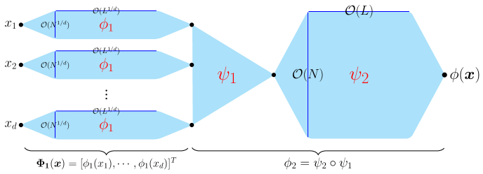
Figure 6: An illustration of the final network architecture with width $\max\{{\mathcal{O}}(dN^{1/d}),\,{\mathcal{O}}(N)\}$ and depth ${\mathcal{O}}(L)$. $\psi_{1}:\mathbb{R}^{d}\to\mathbb{R}$ is a linear function. $\phi_{1}$ and $\psi_{2}$ are implemented via Propositions 3.1 and 3.2, respectively.

Note that $\phi_{1}$ in Figure 6 is a step function mapping $x\in[\tfrac{k}{K},\tfrac{k+1}{K}-\delta\cdot{\mathds{1}}_{\{k\leq K-2\}}]$ to $k$ for each $k\in\{0,1,\cdots,K-1\}$. It can be easily implemented via Proposition 3.1. Clearly, by defining ${\bm{\Phi}}_{1}({\bm{x}})=\big{[}\phi_{1}(x_{1}),\phi_{1}(x_{2}),\cdots,\phi_{1}(x_{d})\big{]}^{T}$, ${\bm{\Phi}}_{1}$ maps ${\bm{x}}\in Q_{\bm{\beta}}$ to ${\bm{\beta}}$.

As shown in Figure 5, we need to design a network to compute $\phi_{2}$ mapping ${\bm{\beta}}\in\{0,1,\cdots,K-1\}^{d}$ approximately to $f({\bm{x}}_{\bm{\beta}})$. To this end, we first construct a linear function $\psi_{1}:\mathbb{R}^{d}\to\mathbb{R}$ mapping ${\bm{\beta}}\in\{0,1,\cdots,K-1\}^{d}$ to $\mathbb{R}$ for the purpose of converting a $d$-dimensional point-fitting problem to a one-dimensional one, and then construct a network to compute $\psi_{2}$ with $\psi_{2}(\psi_{1}({\bm{\beta}}))\approx f({\bm{x}}_{\bm{\beta}})$ via applying Proposition 3.2. Thus, we have $\phi_{2}({\bm{\beta}})\coloneqq\psi_{2}\circ\psi_{1}({\bm{\beta}})\approx f({\bm{x}}_{\bm{\beta}})$ as desired.

Network architectures in Propositions 3.1 and 3.2

To prove Proposition 3.1, we need to construct a ReLU network with width ${\mathcal{O}}(N^{1/d})$ and depth ${\mathcal{O}}(L^{1/d})$ to compute a step function with ${\mathcal{O}}\big{(}(N^{2}L^{2}\ln N)^{1/d}\big{)}$ “steps” outside the trifling region. It is easy to construct a ReLU network with ${\mathcal{O}}(W)$ parameters to compute a step function with $W$ “steps” outside a small region. As we shall see later in Section 4.2, the composition architecture of ReLU networks can help to implement step functions with much more “steps”. Refer to Section 4.2 for the detailed proof of Proposition 3.1.

Proposition 3.2 essentially solves a point-fitting problem with $N^{2}L^{2}\lfloor\log_{3}(N+2)\rfloor$ points via a ReLU network with width ${\mathcal{O}}(N)$ and depth ${\mathcal{O}}(L)$. Set $M=N^{2}L$, ${\widehat{L}}=L\lfloor\log_{3}(N+2)\rfloor$, and represent $j\in\{0,1,\cdots,M{\widehat{L}}-1\}$ via $j=m{\widehat{L}}+k$, where $m\in\{0,1,\cdots,M-1\}$ and $k\in\{0,1,\cdots,{\widehat{L}}-1\}$.

Define $a_{m,k}\coloneqq\lfloor y_{m,k}/\varepsilon\rfloor$ where $y_{m,k}=y_{m{\widehat{L}}+k}$. Then

$$|a_{m,k}\varepsilon-y_{m,k}|=\big{|}\lfloor y_{m,k}/\varepsilon\rfloor\varepsilon-y_{m,k}\big{|}\leq\varepsilon.$$

It suffices to prove $\phi(m,k)=a_{m,k}$. The assumption $|y_{j}-y_{j-1}|\leq\varepsilon$ implies that $b_{m,k}\coloneqq a_{m,k}-a_{m,k-1}\in\{-1,0,1\}$. Thus, there exist $c_{m,k}\in\{0,1\}$ and $d_{m,k}\in\{0,1\}$ such that $b_{m,k}=c_{m,k}-d_{m,k}$.

Note that

$$a_{m,k}=a_{m,0}+\sum_{j=1}^{k}(a_{m,j}-a_{m,j-1})=a_{m,0}+\sum_{j=1}^{k}b_{m,j}=a_{m,0}+\sum_{j=1}^{k}c_{m,j}-\sum_{j=1}^{k}d_{m,j}.$$

It is easy to construct a ReLU network with width ${\mathcal{O}}(N)$ and depth ${\mathcal{O}}(L)$ (${\mathcal{O}}(N^{2}L)$ parameters in total) to compute $\phi_{1}$ such that $\phi_{1}(m)=a_{m,0}$ for each $m\in\{0,1,\cdots,M-1\}$ with $M=N^{2}L$. By the bit extraction technique in [3], one could construct $\phi_{2},\phi_{3}\in\mathcal{NN}(\textnormal{width}\leq{\mathcal{O}}(N);\ \textnormal{depth}\leq{\mathcal{O}}(L))$ such that $\phi_{2}(m,k)=\sum_{j=1}^{k}c_{m,j}$ and $\phi_{3}(m,k)=\sum_{j=1}^{k}d_{m,j}$. Thus, $\phi(m,k)\coloneqq\phi_{1}(m)+\phi_{2}(m,k)-\phi_{3}(m,k)=a_{m,k}$ as desired.

In order to use the bit extraction technique (two types of bits $0$ or $1$) to solve the point-fitting problem, we essentially simplify the target as discussed above. That is,

$$\begin{split}\textnormal{non-negative number $y_{m,k}$}&\longrightarrow\textnormal{integer $a_{m,k}=\lfloor y_{m,k}/\varepsilon\rfloor\mathop{\approx}^{\varepsilon}y_{m,k}$}\\ &\longrightarrow\textnormal{ $b_{m,k}=a_{m,k}-a_{m,k-1}\in\{-1,0,1\}$}\\ &\longrightarrow\textnormal{ $b_{m,k}=c_{m,k}-d_{m,k}$ with $c_{m,k},d_{m,k}\in\{0,1\}$}.\end{split}$$

The detailed proof of Proposition 3.2 can be found in Section 4.3.

3.3 Detailed proof

We essentially construct an almost piecewise constant function implemented by a ReLU network with width ${\mathcal{O}}(N)$ and depth ${\mathcal{O}}(L)$ to approximate $f$. We may assume $f$ is not a constant function since it is a trivial case. Then $\omega_{f}(r)>0$ for any $r>0$. It is clear that $|f(\bm{x})-f({\bm{0}})|\leq\omega_{f}(\sqrt{d})$ for any ${\bm{x}}\in[0,1]^{d}$. Define ${\widetilde{f}}\coloneqq f-f({\bm{0}})+\omega_{f}(\sqrt{d})$, then $0\leq{\widetilde{f}}(\bm{x})\leq 2\omega_{f}(\sqrt{d})$ for any ${\bm{x}}\in[0,1]^{d}$.

Let $M=N^{2}L$, $n=\lfloor\log_{3}(N+2)\rfloor$, $K=\lfloor N^{1/d}\rfloor^{2}\lfloor L^{1/d}\rfloor^{2}\lfloor n^{1/d}\rfloor$, and $\delta$ be an arbitrary number in $(0,\tfrac{1}{3K}]$. The proof can be divided into four steps as follows:

1. Normalize $f$ as ${\widetilde{f}}$, divide $[0,1]^{d}$ into a union of sub-cubes $\{Q_{\bm{\beta}}\}_{\bm{\beta}\in\{0,1,\cdots,K-1\}^{d}}$ and the trifling region $\Omega([0,1]^{d},K,\delta)$, and denote ${\bm{x}}_{\bm{\beta}}$ as the vertex of $Q_{\bm{\beta}}$ with minimum $\|\cdot\|_{1}$ norm;

2. Construct a sub-network to implement a vector function ${\bm{\Phi}}_{1}$ projecting the whole cube $Q_{\bm{\beta}}$ to the $d$-dimensional index ${\bm{\beta}}$ for each ${\bm{\beta}}$, i.e., ${\bm{\Phi}}_{1}({\bm{x}})={\bm{\beta}}$ for all ${\bm{x}}\in Q_{\bm{\beta}}$;

3. Construct a sub-network to implement a function $\phi_{2}$ mapping the index ${\bm{\beta}}$ approximately to ${\widetilde{f}}({\bm{x}}_{\bm{\beta}})$. This core step can be further divided into three sub-steps:

   1. Construct a sub-network to implement $\psi_{1}$ bijectively mapping the index set $\{0,1,\cdots,K-1\}^{d}$ to an auxiliary set $\mathcal{A}_{1}\subseteq\big{\{}\tfrac{j}{2K^{d}}:j=0,1,\cdots,2K^{d}\big{\}}$ defined later (see Figure 8 for an illustration);

   2. Determine a continuous piecewise linear function $g$ with a set of breakpoints $\mathcal{A}_{1}\cup\mathcal{A}_{2}\cup\{1\}$ satisfying: 1) assign the values of $g$ at breakpoints in $\mathcal{A}_{1}$ based on $\{{\widetilde{f}}({\bm{x}}_{\bm{\beta}})\}_{\bm{\beta}}$, i.e., $g\circ\psi_{1}({\bm{\beta}})={\widetilde{f}}({\bm{x}}_{\bm{\beta}})$; 2) assign the values of $g$ at breakpoints in $\mathcal{A}_{2}\cup\{1\}$ to reduce the variation of $g$ for applying Proposition 3.2;

   3. Apply Proposition 3.2 to construct a sub-network to implement a function $\psi_{2}$ approximating $g$ well on $\mathcal{A}_{1}\cup\mathcal{A}_{2}\cup\{1\}$. Then the desired function $\phi_{2}$ is given by $\phi_{2}=\psi_{2}\circ\psi_{1}$ satisfying $\phi_{2}({\bm{\beta}})=\psi_{2}\circ\psi_{1}({\bm{\beta}})\approx g\circ\psi_{1}({\bm{\beta}})={\widetilde{f}}({\bm{x}}_{\bm{\beta}})$;

4. Construct the final network to implement the desired function $\phi$ such that $\phi({\bm{x}})=\phi_{2}\circ{\bm{\Phi}}_{1}({\bm{x}})+f({\bm{0}})-\omega_{f}(\sqrt{d})\approx{\widetilde{f}}({\bm{x}}_{\bm{\beta}})+f({\bm{0}})-\omega_{f}(\sqrt{d})=f({\bm{x}}_{\bm{\beta}})\approx f({\bm{x}})$ for any ${\bm{x}}\in Q_{\bm{\beta}}$ and ${\bm{\beta}}\in\{0,1,\cdots,K-1\}^{d}$.

The details of these steps can be found below.

Step $1\colon$ Divide $[0,1]^{d}$ into $\{Q_{\bm{\beta}}\}_{\bm{\beta}\in\{0,1,\cdots,K-1\}^{d}}$ and $\Omega([0,1]^{d},K,\delta)$.

Define ${\bm{x}}_{\bm{\beta}}\coloneqq{\bm{\beta}}/K$ and

$$Q_{\bm{\beta}}\coloneqq\Big{\{}{\bm{x}}=[x_{1},x_{2},\cdots,x_{d}]^{T}\in[0,1]^{d}:x_{i}\in[\tfrac{\beta_{i}}{K},\tfrac{\beta_{i}+1}{K}-\delta\cdot{\mathds{1}}_{\{\beta_{i}\leq K-2\}}],\quad i=1,2,\cdots,d\Big{\}}$$

for each $d$-dimensional index ${\bm{\beta}}=[\beta_{1},\beta_{2},\cdots,\beta_{d}]^{T}\in\{0,1,\cdots,K-1\}^{d}$. Recall that $\Omega([0,1]^{d},K,\delta)$ is the trifling region defined in Equation (2.1). Apparently, ${\bm{x}}_{\bm{\beta}}$ is the vertex of $Q_{\bm{\beta}}$ with minimum $\|\cdot\|_{1}$ norm and

$$[0,1]^{d}=\big{(}\cup_{\bm{\beta}\in\{0,1,\cdots,K-1\}^{d}}Q_{\bm{\beta}}\big{)}\bigcup\Omega([0,1]^{d},K,\delta).$$

See Figure 7 for illustrations.

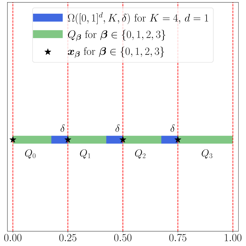
(a)

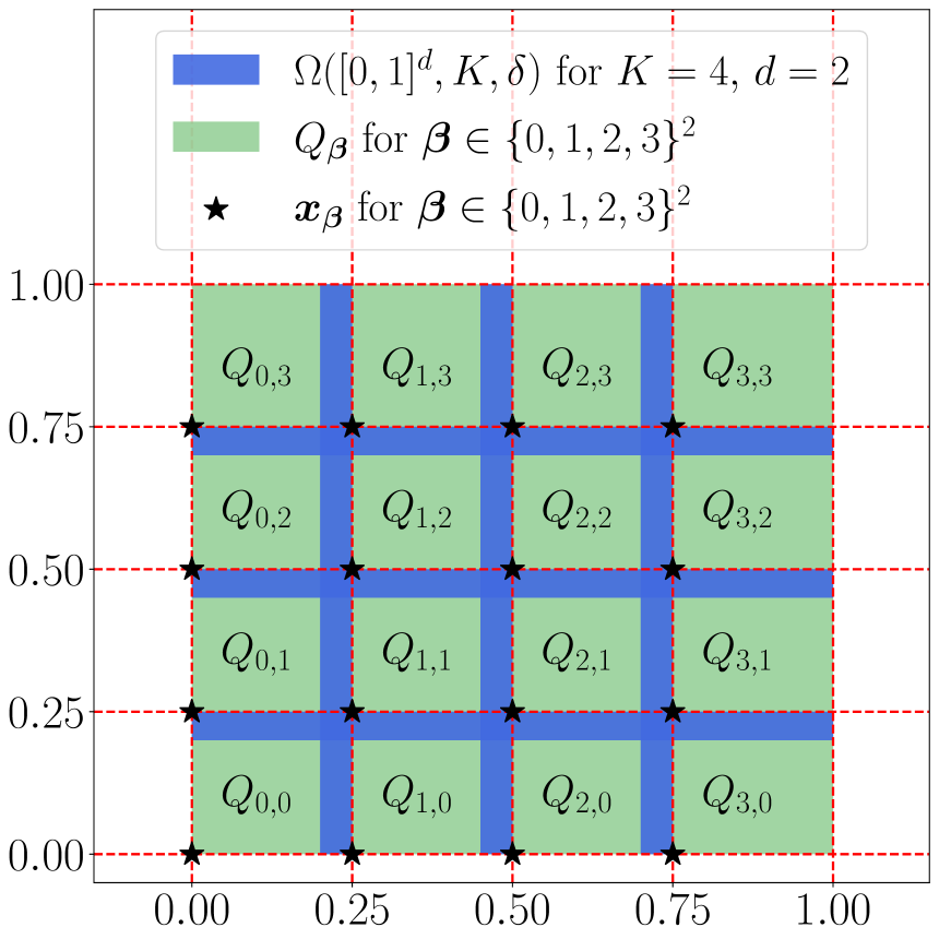
(b)

Figure 7: Illustrations of $\Omega([0,1]^{d},K,\delta)$, $Q_{\bm{\beta}}$, and ${\bm{x}}_{\bm{\beta}}$ for ${\bm{\beta}}\in\{0,1,\cdots,K-1\}^{d}$. (a) $K=4$ and $d=1$. (b) $K=4$ and $d=2$.

Step $2\colon$ Construct ${\bm{\Phi}}_{1}$ mapping ${\bm{x}}\in Q_{\bm{\beta}}$ to ${\bm{\beta}}$.

By Proposition 3.1, there exists $\phi_{1}\in\mathcal{NN}(\textnormal{width}\leq 8\lfloor N^{1/d}\rfloor+3;\ \textnormal{depth}\leq 2\lfloor L^{1/d}\rfloor+5)$ such that

$$\phi_{1}(x)={\color[rgb]{0,0,0}k},\quad\textnormal{if $x\in[\tfrac{k}{K},\tfrac{k+1}{K}-\delta\cdot{\mathds{1}}_{\{k\leq K-2\}}]$,\quad for $k=0,1,\cdots,K-1$.}$$

It follows that $\phi_{1}(x_{i})=\beta_{i}$ if ${\bm{x}}=[x_{1},x_{2},\cdots,x_{d}]^{T}\in Q_{\bm{\beta}}$ for each ${\bm{\beta}}=[\beta_{1},\beta_{2},\cdots,\beta_{d}]^{T}$.

By defining

$${\bm{\Phi}}_{1}({\bm{x}})\coloneqq\big{[}\phi_{1}(x_{1}),\,\phi_{1}(x_{2}),\,\cdots,\,\phi_{1}(x_{d})\big{]}^{T},\quad\textnormal{for any }{\bm{x}}=[x_{1},x_{2},\cdots,x_{d}]^{T}\in\mathbb{R}^{d},$$

we have ${\bm{\Phi}}_{1}({\bm{x}})={\bm{\beta}}$ if ${\bm{x}}\in Q_{\bm{\beta}}$ for each ${\bm{\beta}}\in\{0,1,\cdots,K-1\}^{d}$.

Step $3\colon$ Construct $\phi_{2}$ mapping ${\bm{\beta}}$ approximately to ${\widetilde{f}}({\bm{x}}_{\bm{\beta}})$.

The construction of the sub-network implementing $\phi_{2}$ is essentially based on Proposition 3.2. To meet the requirements of applying Proposition 3.2, we first define two auxiliary sets $\mathcal{A}_{1}$ and $\mathcal{A}_{2}$ as

$$\mathcal{A}_{1}\coloneqq\big{\{}\tfrac{i}{K^{d-1}}+\tfrac{k}{2K^{d}}:i=0,1,\cdots,K^{d-1}{\color[rgb]{0,0,0}-1}\textnormal{\quad and \quad}k=0,1,\cdots,K-1\big{\}}$$

and

$$\mathcal{A}_{2}\coloneqq\big{\{}\tfrac{i}{K^{d-1}}+{\color[rgb]{0,0,0}\tfrac{K+k}{2K^{d}}}:i=0,1,\cdots,K^{d-1}{\color[rgb]{0,0,0}-1}\textnormal{\quad and \quad}k=0,1,\cdots,K-1\big{\}}.$$

Clearly, $\mathcal{A}_{1}\cup\mathcal{A}_{2}\cup\{1\}=\{\tfrac{j}{2K^{d}}:j=0,1,\cdots,2K^{d}\}$ and $\mathcal{A}_{1}\cap\mathcal{A}_{2}=\emptyset$. See Figure 7 for an illustration of $\mathcal{A}_{1}$ and $\mathcal{A}_{2}$. Next, we further divide this step into three sub-steps.

Step $3.1\colon$ Construct $\psi_{1}$ bijectively mapping $\{0,1,\cdots,K-1\}^{d}$ to $\mathcal{A}_{1}$.

Inspired by the binary representation, we define

$$\psi_{1}({\bm{x}})\coloneqq\frac{x_{d}}{2K^{d}}+\sum_{i=1}^{d-1}\frac{x_{i}}{K^{i}},\quad\textnormal{for any ${\bm{x}}=[x_{1},x_{2},\cdots,x_{d}]^{T}\in\mathbb{R}^{d}$.}$$ (3.1)

Then $\psi_{1}$ is a linear function bijectively mapping the index set $\{0,1,\cdots,K-1\}^{d}$ to

$$\begin{split}&\quad\Big{\{}\tfrac{\beta_{d}}{2K^{d}}+\sum_{i=1}^{d-1}\tfrac{\beta_{i}}{K^{i}}:\bm{\beta}\in\{0,1,\cdots,K-1\}^{d}\Big{\}}\\ &=\big{\{}\tfrac{i}{K^{d-1}}+\tfrac{k}{2K^{d}}:i=0,1,\cdots,K^{d-1}{\color[rgb]{0,0,0}-1}\textnormal{\quad and\quad}k=0,1,\cdots,K-1\big{\}}=\mathcal{A}_{1}.\end{split}$$

Step $3.2\colon$ Construct $g$ to satisfy $g\circ\psi_{1}({\bm{\beta}})={\widetilde{f}}({\bm{x}}_{\bm{\beta}})$ and to meet the requirements of applying Proposition 3.2.

Let $g:[0,1]\to\mathbb{R}$ be a continuous piecewise linear function with a set of breakpoints $\left\{\tfrac{j}{2K^{d}}:j=0,1,\cdots,2K^{d}\right\}=\mathcal{A}_{1}\cup\mathcal{A}_{2}\cup\{1\}$ and the values of $g$ at these breakpoints satisfy the following properties:

• The values of $g$ at the breakpoints in $\mathcal{A}_{1}=\big{\{}\psi_{1}({\bm{\beta}}):\bm{\beta}\in\{0,1,\cdots,K-1\}^{d}\big{\}}$ are set as

  $$g(\psi_{1}({\bm{\beta}}))={\widetilde{f}}({\bm{x}}_{\bm{\beta}}),\quad\textnormal{for any $\bm{\beta}\in\{0,1,\cdots,K-1\}^{d}$;}$$ (3.2)

• At the breakpoint $1$, let $g(1)={\widetilde{f}}(\bm{1})$, where $\bm{1}=[1,1,\cdots,1]^{T}\in\mathbb{R}^{d}$;

• The values of $g$ at the breakpoints in $\mathcal{A}_{2}$ are assigned to reduce the variation of $g$, which is a requirement of applying Proposition 3.2. Note that

  $$\big{\{}\tfrac{i}{K^{d-1}}-\tfrac{K+1}{2K^{d}},\ \tfrac{i}{K^{d-1}}\big{\}}\subseteq\mathcal{A}_{1}\cup\{1\},\quad\textnormal{for $i=1,2,\cdots,K^{d-1}$,}$$

  implying the values of $g$ at $\tfrac{i}{K^{d-1}}-\tfrac{K+1}{2K^{d}}$ and $\tfrac{i}{K^{d-1}}$ have been assigned for $i=1,2,\cdots,K^{d-1}$. Thus, the values of $g$ at the breakpoints in $\mathcal{A}_{2}$ can be successfully assigned by letting $g$ linear on each interval $[\tfrac{i}{K^{d-1}}-\tfrac{K+1}{2K^{d}},\,\tfrac{i}{K^{d-1}}]$ for $i=1,2,\cdots,K^{d-1}$, since $\mathcal{A}_{2}\subseteq\bigcup_{i=1}^{K^{d-1}}[\tfrac{i}{K^{d-1}}-\tfrac{K+1}{2K^{d}},\,\tfrac{i}{K^{d-1}}]$. See Figure 8 for an illustration.

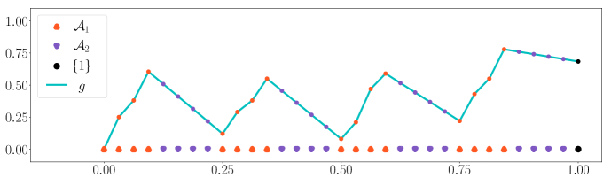
Figure 8: An illustration of $\mathcal{A}_{1}$, $\mathcal{A}_{2}$, $\{1\}$, and $g$ for $d=2$ and $K=4$.

Apparently, such a function $g$ exists (see Figure 8 for an example) and satisfies

$$\left|g(\tfrac{j}{2K^{d}})-g(\tfrac{j-1}{2K^{d}})\right|\leq\max\big{\{}\omega_{f}(\tfrac{1}{K}),\omega_{f}({\sqrt{d}})/K\big{\}}\leq\omega_{f}(\tfrac{\sqrt{d}}{K}),\quad\textnormal{for }j=1,2,\cdots,2K^{d},$$

and

$$0\leq g(\tfrac{j}{2K^{d}})\leq 2\omega_{f}(\sqrt{d}),\quad\textnormal{for}\ j=0,1,\cdots,2K^{d}.$$

Step $3.3\colon$ Construct $\psi_{2}$ approximating $g$ well on $\mathcal{A}_{1}\cup\mathcal{A}_{2}\cup\{1\}$.

Note that

$$2K^{d}=2\big{(}\lfloor N^{1/d}\rfloor^{2}\lfloor L^{1/d}\rfloor^{2}\lfloor n^{1/d}\rfloor\big{)}^{d}\leq 2\big{(}N^{2}L^{2}n\big{)}\leq{N}^{2}\lceil\sqrt{2}L\rceil^{2}\lfloor\log_{3}(N+2)\rfloor.$$

By Proposition 3.2 (set $y_{j}=g(\tfrac{j}{2K^{2}})$ and $\varepsilon=\omega_{f}(\tfrac{\sqrt{d}}{K})>0$ therein), there exists

$$\begin{split}{\widetilde{\psi}}_{2}\in\mathcal{NN}(\textnormal{\#input}=1;\ \textnormal{width}\leq 16N+30;\ \textnormal{depth}\leq 6\lceil\sqrt{2}L\rceil+10;\ \textnormal{\#output}=1)\end{split}$$

such that

$$|{\widetilde{\psi}}_{2}(j)-g(\tfrac{j}{2K^{d}})|\leq\omega_{f}(\tfrac{\sqrt{d}}{K}),\quad\textnormal{for }j=0,1,\cdots,2K^{d}-1,$$

and

$$\begin{split}0\leq{\widetilde{\psi}}_{2}(x)\leq\max\{g(\tfrac{j}{2K^{d}}):j=0,1,\cdots,2K^{d}-1\}\leq 2\omega_{f}(\sqrt{d}),\quad\textnormal{for any $x\in\mathbb{R}$.}\end{split}$$

By defining $\psi_{2}(x)\coloneqq{\widetilde{\psi}}_{2}(2K^{d}x)$ for any $x\in\mathbb{R}$, we have $\psi_{2}\in\mathcal{NN}(\textnormal{\#input}=1;\ \textnormal{width}\leq 16N+30;\ \textnormal{depth}\leq 6\lceil\sqrt{2}L\rceil+10;\ \textnormal{\#output}=1)$,

$$\begin{split}0\leq\psi_{2}(x)={\widetilde{\psi}}_{2}(2K^{d}x)\leq 2\omega_{f}(\sqrt{d}),\quad\textnormal{for any }x\in\mathbb{R},\end{split}$$ (3.3)

and

$$|\psi_{2}(\tfrac{j}{2K^{d}})-g(\tfrac{j}{2K^{d}})|=|{\widetilde{\psi}}_{2}(j)-g(\tfrac{j}{2K^{d}})|\leq\omega_{f}(\tfrac{\sqrt{d}}{K}),\quad\textnormal{for $j=0,1,\cdots,2K^{d}-1.$}$$ (3.4)

Let us end Step $3$ by defining the desired function $\phi_{2}$ as $\phi_{2}\coloneqq\psi_{2}\circ\psi_{1}$. Note that $\psi_{1}:\mathbb{R}^{d}\to\mathbb{R}$ is a linear function and $\psi_{2}\in\mathcal{NN}(\textnormal{\#input}=1;\ \textnormal{width}\leq 16N+30;\ \textnormal{depth}\leq 6\lceil\sqrt{2}L\rceil+10;\ \textnormal{\#output}=1)$. Thus, $\phi_{2}\in\mathcal{NN}(\textnormal{\#input}=1;\ \textnormal{width}\leq 16N+30;\ \textnormal{depth}\leq 6\lceil\sqrt{2}L\rceil+10;\ \textnormal{\#output}=1)$. By Equations (3.2) and (3.4), we have

$$\begin{split}|\phi_{2}({\bm{\beta}})-{\widetilde{f}}({\bm{x}}_{\bm{\beta}})|=\left|\psi_{2}(\psi_{1}({\bm{\beta}}))-g(\psi_{1}({\bm{\beta}}))\right|\leq\omega_{f}(\tfrac{\sqrt{d}}{K}),\end{split}$$ (3.5)

for any ${\bm{\beta}}\in\{0,1,\cdots,K-1\}^{d}$. Equation (3.3) and $\phi_{2}=\psi_{2}\circ\psi_{1}$ implies

$$\begin{split}0\leq\phi_{2}({\bm{x}})\leq 2\omega_{f}(\sqrt{d}),\quad\textnormal{for any }{\bm{x}}\in\mathbb{R}^{d}.\end{split}$$ (3.6)

Step $4\colon$ Construct the final network to implement the desired function $\phi$.

Define $\phi\coloneqq\phi_{2}\circ{\bm{\Phi}}_{1}+f({\bm{0}})-\omega_{f}(\sqrt{d})$. Since $\phi_{1}\in\mathcal{NN}(\textnormal{width}\leq 8\lfloor N^{1/d}\rfloor+3;\ \textnormal{depth}\leq 2\lfloor L^{1/d}\rfloor+5])$, we have ${\bm{\Phi}}_{1}\in\mathcal{NN}(\textnormal{\#input}=d;\ \textnormal{width}\leq 8d\lfloor N^{1/d}\rfloor+3d;\ \textnormal{depth}\leq 2L+5;\ \textnormal{\#output}=d)$. It follows from the fact $\lceil\sqrt{2}L\rceil\leq\lceil\tfrac{3}{2}L\rceil\leq\tfrac{3}{2}L+\tfrac{1}{2}$ that $6\lceil\sqrt{2}L\rceil+10\leq 9L+13$, implying

$$\begin{split}\phi_{2}&\in\mathcal{NN}(\textnormal{\#input}=1;\ \textnormal{width}\leq 16N+30;\ \textnormal{depth}\leq 6\lceil\sqrt{2}L\rceil+10;\ \textnormal{\#output}=1)\\ &\subseteq\mathcal{NN}(\textnormal{\#input}=1;\ \textnormal{width}\leq 16N+30;\ \textnormal{depth}\leq 9L+13;\ \textnormal{\#output}=1).\end{split}$$

Thus, $\phi=\phi_{2}\circ{\bm{\Phi}}_{1}+f({\bm{0}})-\omega_{f}(\sqrt{d})$ is in

$$\begin{split}\mathcal{NN}\big{(}\textnormal{width}\leq\max\{8d\lfloor N^{1/d}\rfloor+3d,16N+30\};\ \textnormal{depth}\leq(2L+5)+(9L+13)=11L+18\big{)}.\end{split}$$

Now let us estimate the approximation error. Note that $f={\widetilde{f}}+f({\bm{0}})-\omega_{f}(\sqrt{d})$. By Equation (3.5), for any ${\bm{x}}\in Q_{\bm{\beta}}$ and ${\bm{\beta}}\in\{0,1,\cdots,K-1\}^{d}$, we have

$$\begin{split}|f({\bm{x}})-\phi({\bm{x}})|&=|{\widetilde{f}}({\bm{x}})-\phi_{2}({\bm{\Phi}}_{1}({\bm{x}}))|=|{\widetilde{f}}({\bm{x}})-\phi_{2}({\bm{\beta}})|\\ &\leq|{\widetilde{f}}({\bm{x}})-{\widetilde{f}}({\bm{x}}_{\bm{\beta}})|+|{\widetilde{f}}({\bm{x}}_{\bm{\beta}})-\phi_{2}({\bm{\beta}})|\\ &\leq\omega_{f}(\tfrac{\sqrt{d}}{K})+\omega_{f}(\tfrac{\sqrt{d}}{K})\leq 2\omega_{f}\Big{(}64\sqrt{d}\big{(}N^{2}L^{2}\log_{3}(N+2)\big{)}^{-1/d}\Big{)},\end{split}$$

where the last inequality comes from the fact

$$\begin{split}K=\lfloor N^{1/d}\rfloor^{2}\lfloor L^{1/d}\rfloor^{2}\lfloor n^{1/d}\rfloor&\geq\tfrac{N^{2/d}L^{2/d}n^{1/d}}{32}=\tfrac{N^{2/d}L^{2/d}\lfloor\log_{3}(N+2)\rfloor^{1/d}}{32}\geq\tfrac{(N^{2}L^{2}\log_{3}(N+2))^{1/d}}{64},\end{split}$$

for any $N,L\in\mathbb{N}^{+}$. Recall the fact $\omega_{f}(j\cdot r)\leq j\cdot\omega_{f}(r)$ for any $j\in\mathbb{N}^{+}$ and $r\in[0,\infty)$. Therefore, for any ${\bm{x}}\in\bigcup_{\bm{\beta}\in\{0,1,\cdots,K-1\}^{d}}Q_{\bm{\beta}}{\color[rgb]{0,0,0}=}[0,1]^{d}\backslash\Omega([0,1]^{d},K,\delta)$, we have

$$\begin{split}|f({\bm{x}})-\phi({\bm{x}})|&\leq 2\omega_{f}\Big{(}64\sqrt{d}\big{(}N^{2}L^{2}\log_{3}(N+2)\big{)}^{-1/d}\Big{)}\\ &\leq 2\Big{\lceil}64\sqrt{d}\Big{\rceil}\omega_{f}\Big{(}\big{(}N^{2}L^{2}\log_{3}(N+2)\big{)}^{-1/d}\Big{)}\\ &\leq 130\sqrt{d}\,\omega_{f}\Big{(}\big{(}N^{2}L^{2}\log_{3}(N+2)\big{)}^{-1/d}\Big{)}.\end{split}$$

It remains to show the upper bound of $\phi$. By Equation (3.6) and $\phi=\phi_{2}\circ{\bm{\Phi}}_{1}+f({\bm{0}})-\omega_{f}(\sqrt{d})$, it holds that $\|\phi\|_{L^{\infty}(\mathbb{R}^{d})}\leq|f({\bm{0}})|+\omega_{f}(\sqrt{d})$. Thus, we finish the proof.

4 Proofs of propositions in Section 3.1

In this section, we will prove Propositions 3.1 and 3.2. We first introduce several basic results of ReLU networks. Next, we prove these two propositions based on these basic results.

4.1 Basic results of ReLU networks

To simplify the proofs of two propositions in Section 3.1, we introduce three lemmas below, which are basic results of ReLU networks

Lemma 4.1.

For any $N_{1},N_{2}\in\mathbb{N}^{+}$, given $N_{1}(N_{2}+1)+1$ samples $(x_{i},y_{i})\in\mathbb{R}^{2}$ with $x_{0}<x_{1}<\cdots<x_{N_{1}(N_{2}+1)}$ and $y_{i}\geq 0$ for $i=0,1,\cdots,N_{1}(N_{2}+1)$, there exists $\phi\in\mathcal{NN}(\textnormal{\#input}=1;\ \textnormal{width\hskip 0.5ptvec}=[2N_{1},2N_{2}+1];\ \textnormal{\#output}=1)$ satisfying the following conditions.

1. $\phi(x_{i})=y_{i}$ for $i=0,1,\cdots,N_{1}(N_{2}+1)$.

2. $\phi$ is linear on each interval $[x_{i-1},x_{i}]$ for $i\notin\{(N_{2}+1)j:j=1,2,\cdots,N_{1}\}$.

Lemma 4.2.

Given any $N,L,d\in\mathbb{N}^{+}$, it holds that

$$\begin{split}&\quad\,\mathcal{NN}(\textnormal{\#input}=d;\ \textnormal{width\hskip 0.5ptvec}=[N,NL];\ \textnormal{\#output}=1)\\ &\subseteq\mathcal{NN}(\textnormal{\#input}=d;\ \textnormal{width}\leq 2N+2;\ \textnormal{depth}\leq L+1;\ \textnormal{\#output}=1).\end{split}$$

Lemma 4.3.

For any $n\in\mathbb{N}^{+}$, it holds that

$$\textnormal{CPwL}\big{(}\mathbb{R},n\big{)}\subseteq\mathcal{NN}(\textnormal{\#input}=1;\ \textnormal{width\hskip 0.5ptvec}=[n+1];\ \textnormal{\#output}=1).$$ (4.1)

Lemma 4.1 is a part of Theorem $3.2$ in [44] or Lemma $2.2$ in [32]. Lemma 4.1 is Theorem $3.1$ in [44] or Lemma $3.4$ in [32]. It remains to prove Lemma 4.3.

Proof of Lemma 4.3.

We use the mathematical induction to prove Equation (4.1). First, consider the case $n=1$. Given any $f\in\textnormal{CPwL}\big{(}\mathbb{R},1\big{)}$, there exist $a_{1},a_{2},x_{0}\in\mathbb{R}$ such that

$$f(x)=\left\{\begin{array}[]{ll}a_{1}(x-x_{0})+f(x_{0}),&\textnormal{if \ }x\geq x_{0},\\ a_{2}(x_{0}-x)+f(x_{0}),&\textnormal{if \ }x<x_{0}.\\ \end{array}\right.$$

Thus, $f(x)=a_{1}\sigma(x-x_{0})+a_{2}\sigma(x_{0}-x)+f(x_{0})$ for any $x\in\mathbb{R}$, implying

$$f\in\mathcal{NN}(\textnormal{\#input}=1;\ \textnormal{width\hskip 0.5ptvec}=[2];\ \textnormal{\#output}=1).$$

Thus, Equation (4.1) holds for $n=1$.

Now assume Equation (4.1) holds for $n=k\in\mathbb{N}^{+}$, we would like to show it is also true for $n=k+1$. Given any $f\in\textnormal{CPwL}\big{(}\mathbb{R},k+1\big{)}$, we may assume the biggest breakpoint of $f$ is $x_{0}$ since it is trivial for the case that $f$ has no breakpoint. Denote the slopes of the linear pieces left and right next to $x_{0}$ by $a_{1}$ and $a_{2}$, respectively. Define

$${\widetilde{f}}(x)\coloneqq f(x)-(a_{2}-a_{1})\sigma(x-x_{0}),\quad\textnormal{ for any $x\in\mathbb{R}$.}$$

Then ${\widetilde{f}}$ has at most $k$ breakpoints. By the induction hypothesis, we have

$${\widetilde{f}}\in\textnormal{CPwL}\big{(}\mathbb{R},k\big{)}\subseteq\mathcal{NN}(\textnormal{\#input}=1;\ \textnormal{width\hskip 0.5ptvec}=[k+1];\ \textnormal{\#output}=1).$$

Thus, there exist $w_{0,j},b_{0,j},w_{1,j},b_{1}$ for $j=1,2,\cdots,k+1$ such that

$${\widetilde{f}}(x)=\sum_{j=1}^{k+1}w_{1,j}\sigma(w_{0,j}x+b_{0,j})+b_{1},\quad\textnormal{for any $x\in\mathbb{R}$.}$$

Therefore, for any $x\in\mathbb{R}$, we have

$$f(x)=(a_{2}-a_{1})\sigma(x-x_{0})+{\widetilde{f}}(x)=(a_{2}-a_{1})\sigma(x-x_{0})+\sum_{j=1}^{k+1}w_{1,j}\sigma(w_{0,j}x+b_{0,j})+b_{1},$$

implying $f\in\mathcal{NN}(\textnormal{\#input}=1;\ \textnormal{width\hskip 0.5ptvec}=[k+2];\ \textnormal{\#output}=1)$. Thus, Equation (4.1) holds for $k+1$, which means we finish the induction process. So we complete the proof. ∎

4.2 Proof of Proposition 3.1

Now, let us present the detailed proof of Proposition 3.1. Denote $K={\widetilde{M}}\cdot{\widetilde{L}}$, where ${\widetilde{M}}=\lfloor N^{1/d}\rfloor^{2}\lfloor L^{1/d}\rfloor$, $n=\lfloor\log_{3}(N+2)\rfloor$, and ${\widetilde{L}}=\lfloor L^{1/d}\rfloor\lfloor n^{1/d}\rfloor$. Consider the sample set

$$\begin{split}\big{\{}(1,{\widetilde{M}}-1),(2,0)\big{\}}&\bigcup\big{\{}(\tfrac{m}{{\widetilde{M}}},m):m=0,1,\cdots,{\widetilde{M}}-1\big{\}}\\ &\bigcup\big{\{}(\tfrac{m+1}{{\widetilde{M}}}-\delta,m):m=0,1,\cdots,{\widetilde{M}}-2\big{\}}.\end{split}$$

Its size is

$$2{\widetilde{M}}+1=2\lfloor N^{1/d}\rfloor^{2}\lfloor L^{1/d}\rfloor+1=\lfloor N^{1/d}\rfloor\cdot\Big{(}\big{(}2\lfloor N^{1/d}\rfloor\lfloor L^{1/d}\rfloor-1\big{)}+1\Big{)}+1.$$

By Lemma 4.1 (set $N_{1}=\lfloor N^{1/d}\rfloor$ and $N_{2}=2\lfloor N^{1/d}\rfloor\lfloor L^{1/d}\rfloor-1$ therein), there exists

$$\begin{split}\phi_{1}&\in\mathcal{NN}\big{(}\textnormal{width\hskip 0.5ptvec}=\big{[}2\lfloor N^{1/d}\rfloor,2(2\lfloor N^{1/d}\rfloor\lfloor L^{1/d}\rfloor-1)+1\big{]}\big{)}\\ &=\mathcal{NN}\big{(}\textnormal{width\hskip 0.5ptvec}=\big{[}2\lfloor N^{1/d}\rfloor,4\lfloor N^{1/d}\rfloor\lfloor L^{1/d}\rfloor-1\big{]}\big{)}\end{split}$$

such that

• $\phi_{1}(\tfrac{{\widetilde{M}}-1}{{\widetilde{M}}})=\phi_{1}(1)={\widetilde{M}}-1$ and $\phi_{1}(\tfrac{m}{{\widetilde{M}}})=\phi_{1}(\tfrac{m+1}{{\widetilde{M}}}-\delta)=m$ for $m=0,1,\cdots,{\widetilde{M}}-2$.

• $\phi_{1}$ is linear on $[\tfrac{{\widetilde{M}}-1}{{\widetilde{M}}},1]$ and each interval $[\tfrac{m}{{\widetilde{M}}},\tfrac{m+1}{{\widetilde{M}}}-\delta]$ for $m=0,1,\cdots,{\widetilde{M}}-2$.

Then, for $m=0,1,\cdots,{\widetilde{M}}-1$, we have

$$\phi_{1}(x)=m,\quad\textnormal{for any}\ x\in[\tfrac{m}{{\widetilde{M}}},\tfrac{m+1}{{\widetilde{M}}}-\delta\cdot{\mathds{1}}_{\{m\leq{\widetilde{M}}-2\}}].$$ (4.2)

Now consider another sample set

$$\begin{split}\big{\{}(\tfrac{1}{{\widetilde{M}}},{\widetilde{L}}-1),(2,0)\big{\}}&\bigcup\big{\{}(\tfrac{\ell}{{\widetilde{M}}{\widetilde{L}}},\ell):\ell=0,1,\cdots,{\widetilde{L}}-1\big{\}}\\ &\bigcup\big{\{}(\tfrac{\ell+1}{{\widetilde{M}}{\widetilde{L}}}-\delta,\ell):\ell=0,1,\cdots,{\widetilde{L}}-2\big{\}}.\end{split}$$

Its size is

$$2{\widetilde{L}}+1=2\lfloor L^{1/d}\rfloor\lfloor n^{1/d}\rfloor+1=\lfloor n^{1/d}\rfloor\cdot\big{(}(2\lfloor L^{1/d}\rfloor-1)+1\big{)}+1.$$

By Lemma 4.1 (set $N_{1}=\lfloor n^{1/d}\rfloor$ and $N_{2}=2\lfloor L^{1/d}\rfloor-1$ therein), there exists

$$\begin{split}\phi_{2}&\in\mathcal{NN}\big{(}\textnormal{width\hskip 0.5ptvec}=\big{[}2\lfloor n^{1/d}\rfloor,2(2\lfloor L^{1/d}\rfloor-1)+1\big{]}\big{)}\\ &=\mathcal{NN}\big{(}\textnormal{width\hskip 0.5ptvec}=\big{[}2\lfloor n^{1/d}\rfloor,4\lfloor L^{1/d}\rfloor-1\big{]}\big{)}\end{split}$$

such that

• $\phi_{2}(\tfrac{{\widetilde{L}}-1}{{\widetilde{M}}{\widetilde{L}}})=\phi_{2}(\tfrac{1}{{\widetilde{M}}})={\widetilde{L}}-1$ and $\phi_{2}(\tfrac{\ell}{{\widetilde{M}}{\widetilde{L}}})=\phi_{2}(\tfrac{\ell+1}{{\widetilde{M}}{\widetilde{L}}}-\delta)=\ell$ for $\ell=0,1,\cdots,{\widetilde{L}}-2$.

• $\phi_{2}$ is linear on $[\tfrac{{\widetilde{L}}-1}{{\widetilde{M}}{\widetilde{L}}},\tfrac{1}{{\widetilde{M}}}]$ and each interval $[\tfrac{\ell}{{\widetilde{M}}{\widetilde{L}}},\tfrac{\ell+1}{{\widetilde{M}}{\widetilde{L}}}-\delta]$ for $\ell=0,1,\cdots,{\widetilde{L}}-2$.

It follows that, for $m=0,1,\cdots,{\widetilde{M}}-1$ and $\ell=0,1,\cdots,{\widetilde{L}}-1$,

$$\phi_{2}(x-\tfrac{m}{{\widetilde{M}}})=\ell,\quad\textnormal{for any}\ x\in[\tfrac{m{\widetilde{L}}+\ell}{{\widetilde{M}}{\widetilde{L}}},\tfrac{m{\widetilde{L}}+\ell+1}{{\widetilde{M}}{\widetilde{L}}}-\delta\cdot{\mathds{1}}_{\{\ell\leq{\widetilde{L}}-2\}}].$$ (4.3)

$K={\widetilde{M}}\cdot{\widetilde{L}}$ implies any $k\in\{0,1,\cdots,K-1\}$ can be unique represented by $k=m{\widetilde{L}}+\ell$ for $m\in\{0,1,\cdots,{\widetilde{M}}-1\}$ and $\ell\in\{0,1,\cdots,{\widetilde{L}}-1\}$. Then the desired function $\phi$ can be implemented by a ReLU network shown in Figure 9.

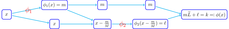
Figure 9: An illustration of the network architecture implementing $\phi$ based on Equations (4.2) and (4.3) for $x\in[\tfrac{k}{K},\tfrac{k+1}{K}-\delta\cdot{\mathds{1}}_{\{k\leq K-2\}}]=[\tfrac{mL+\ell}{{\widetilde{M}}{\widetilde{L}}},\tfrac{mL+\ell+1}{{\widetilde{M}}{\widetilde{L}}}-\delta\cdot{\mathds{1}}_{\{m\leq{\widetilde{M}}-2\textnormal{ or }\ell\leq{\widetilde{L}}-2\}}]$, where $k=m{\widetilde{L}}+\ell$ for $m=0,1,\cdots,{\widetilde{M}}-1$ and $\ell=0,1,\cdots,{\widetilde{L}}-1$.

Clearly,

$$\phi(x)=k,\quad\textnormal{if $x\in[\tfrac{k}{K},\tfrac{k+1}{K}-\delta\cdot{\mathds{1}}_{\{k\leq K-2\}}]$,\quad for any $k\in\{0,1,\cdots,K-1\}.$}$$

By Lemma 4.2, we have

$$\begin{split}\phi_{1}&\in\mathcal{NN}\big{(}\textnormal{\#input}=1;\ \textnormal{width\hskip 0.5ptvec}=\big{[}2\lfloor N^{1/d}\rfloor,4\lfloor N^{1/d}\rfloor\lfloor L^{1/d}\rfloor-1\big{]};\ \textnormal{\#output}=1\big{)}\\ &\subseteq\mathcal{NN}\big{(}\textnormal{\#input}=1;\ \textnormal{width}\leq 8\lfloor N^{1/d}\rfloor+2;\ \textnormal{depth}\leq\lfloor L^{1/d}\rfloor+1;\ \textnormal{\#output}=1\big{)}\end{split}$$

and

$$\begin{split}\phi_{2}&\in\mathcal{NN}\big{(}\textnormal{\#input}=1;\ \textnormal{width\hskip 0.5ptvec}=\big{[}2\lfloor n^{1/d}\rfloor,4\lfloor L^{1/d}\rfloor-1\big{]};\ \textnormal{\#output}=1\big{)}\\ &\subseteq\mathcal{NN}\big{(}\textnormal{\#input}=1;\ \textnormal{width}\leq 8\lfloor n^{1/d}\rfloor+2;\ \textnormal{depth}\leq\lfloor L^{1/d}\rfloor+1;\ \textnormal{\#output}=1\big{)}.\end{split}$$

Recall that $n=\lfloor\log_{3}(N+2)\rfloor\leq N$. It follows from Figure 9 that $\phi$ can be implemented by a ReLU network with width

$$\max\big{\{}8\lfloor N^{1/d}\rfloor+2+1,8\lfloor n^{1/d}\rfloor+2+1\big{\}}=8\lfloor N^{1/d}\rfloor+3$$

and depth

$$(\lfloor L^{1/d}\rfloor+1)+2+(\lfloor L^{1/d}\rfloor+1)+1=2\lfloor L^{1/d}\rfloor+5.$$

So we finish the proof.

4.3 Proof of Proposition 3.2

The proof of Proposition 3.2 is based on the bit extraction technique in [3, 13]. To simplify the proof, we first prove Lemmas 4.4, 4.5, 4.6, and 4.7, which serve as four important intermediate steps. Next, we will apply Lemma 4.7 to prove Proposition 3.2. In fact, we modify this technique to extract the sum of many bits rather than one bit and this modification can be summarized in Lemmas 4.4 and 4.5 below.

Lemma 4.4.

For any $n\in\mathbb{N}^{+}$, there exists a function $\phi$ in

$$\mathcal{NN}\big{(}\textnormal{\#input}=2;\ \textnormal{width}\leq(n+1)2^{n+1};\ \textnormal{depth}\leq 3;\ \textnormal{\#output}=1\big{)}$$

such that: Given any $\theta_{j}\in\{0,1\}$ for $j=1,2,\cdots,n$, we have

$$\phi(\textnormal{bin}\hskip 1.2pt0.\theta_{1}\theta_{2}\cdots\theta_{n},\,i)=\sum_{j=1}^{i}\theta_{j},\quad\textnormal{for any $i\in\{0,1,2,\cdots,n\}$}.\,$$

Proof.

Set $\theta=\textnormal{bin}\hskip 1.2pt0.\theta_{1}\theta_{2}\cdots\theta_{n}$. Clearly,

$$\theta_{j}={\lfloor 2^{j}\theta\rfloor}\big{/}{2}-\lfloor 2^{j-1}\theta\rfloor,\quad\textnormal{for any $j\in\{1,2,\cdots,n\}$.}$$

We shall use a ReLU network to replace $\lfloor\cdot\rfloor$. Let $g\in\textnormal{CPwL}(\mathbb{R},2^{n+1}-2)$ be the function satisfying two conditions:

• $g$ matches set of samples

  $$\bigcup_{k=0}^{2^{n}-1}\big{\{}(k,k),(k+1-\delta,k)\big{\}},\quad\textnormal{where $\delta=2^{-(n+1)}$;}$$

• The breakpoint set of $g$ is

  $$\Big{(}\bigcup_{k=0}^{2^{n}-1}\big{\{}k,k+1-\delta\big{\}}\Big{)}\Big{\backslash}\Big{(}\{0\}\bigcup\{2^{n}-\delta\}\Big{)}.$$

Then $g(x)=\lfloor x\rfloor$ for any $x\in\bigcup_{k=0}^{2^{n}-1}[k,k+1-\delta]$. Clearly, $\theta=\textnormal{bin}\hskip 1.2pt0.\theta_{1}\theta_{2}\cdots\theta_{n}$ implies

$$2^{j}\theta\in\bigcup_{k=0}^{2^{n}-1}[k,k+1-\delta],\quad\textnormal{ for any $j\in\{0,1,2,\cdots,n\}$}.$$

Thus,

$$\theta_{j}={\lfloor 2^{j}\theta\rfloor}\big{/}{2}-\lfloor 2^{j-1}\theta\rfloor\,=\,{g(2^{j}\theta)}\big{/}{2}-g(2^{j-1}\theta),\quad\textnormal{for any $j\in\{1,2,\cdots,n\}$.}$$ (4.4)

It is easy to design a ReLU network to output $\theta_{1},\theta_{2},\cdots,\theta_{n}$ by Equation (4.4) when using $\theta=\textnormal{bin}\hskip 1.2pt0.\theta_{1}\theta_{2}\cdots\theta_{n}$ as the input. However, it is highly non-trivial to construct a ReLU network to output $\sum_{j=1}^{i}\theta_{j}$ with another input $i$, since many operations like multiplication and comparison are not allowed in designing ReLU networks. Now let us establish a formula to represent $\sum_{j=1}^{i}\theta_{j}$ in a form of a ReLU network as follows.

Define $\mathcal{T}(n)\coloneqq\sigma(n+1)-\sigma(n)=\left\{\begin{matrix}[l]1,&n\geq 0,\\ 0,&n<0\end{matrix}\right.$ for any integer $n$. Then, by Equation (4.4) and the fact $x_{1}x_{2}=\sigma(x_{1}+x_{2}-1)$ for any $x_{1},x_{2}\in\{0,1\}$, we have, for $i=0,1,2,\cdots,n$,

$$\begin{split}\sum_{j=1}^{i}\theta_{j}=\sum_{j=1}^{n}\theta_{j}\cdot\mathcal{T}(i-j)&=\sum_{j=1}^{n}\sigma\Big{(}\theta_{j}+\mathcal{T}(i-j)-1\Big{)}\\ &=\sum_{j=1}^{n}\sigma\Big{(}\theta_{j}+\sigma(i-j+1)-\sigma(i-j)-1\Big{)}\\ &=\sum_{j=1}^{n}\sigma\Big{(}{g(2^{j}\theta)}\big{/}{2}-g(2^{j-1}\theta)+\sigma(i-j+1)-\sigma(i-j)-1\Big{)}.\end{split}$$

Define

$$\begin{split}z_{i,j}&\coloneqq\sigma\Big{(}g(2^{j}\theta)\big{/}2-g(2^{j-1}\theta)+\sigma(i-j+1)-\sigma(i-j)-1\Big{)},\end{split}$$ (4.5)

for any $i,j\in\{0,1,2,\cdots,n\}$. Then the goal is to design $\phi$ satisfying

$$\phi(\theta,i)=\sum_{j=1}^{i}\theta_{j}=\sum_{j=1}^{n}z_{i,j},\quad\textnormal{ for any $i\in\{0,1,2,\cdots,n\}$.}$$ (4.6)

See Figure 10 for the network architecture implementing the desired function $\phi$.

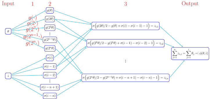
Figure 10: An illustration of the network implementing the desired function $\phi$ with the input $[\theta,i]^{T}=[\textnormal{bin}\hskip 1.2pt0.\theta_{1}\theta_{2}\cdots\theta_{n},\,i]^{T}$ for any $i\in\{0,1,2,\cdots,n\}$ and $\theta_{1},\theta_{2},\cdots,\theta_{n}\in\{0,1\}$. $g(2^{j}\cdot)$ can be implemented by a one-hidden-layer network with width $2^{n+1}-1$ for each $j\in\{0,1,2,\cdots,n\}$. The red numbers above the architecture indicate the order of hidden layers. The network architecture is essentially determined by Equations (4.5) and (4.6), which are valid no matter what $\theta_{1},\theta_{2},\cdots,\theta_{n}\in\{0,1\}$ are. Thus, the desired function $\phi$ is independent of $\theta_{1},\theta_{2},\cdots,\theta_{n}\in\{0,1\}$. We omit ReLU ($\sigma$) for a neuron if its output is non-negative without ReLU. Such a simplification is applied to similar figures in this paper.

By Lemma 4.3, we have

$$g\in\textnormal{CPwL}(\mathbb{R},2^{n+1}-2)\subseteq\mathcal{NN}\big{(}\textnormal{\#input}=1;\ \textnormal{width\hskip 0.5ptvec}=[2^{n+1}-1];\ \textnormal{\#output}=1\big{)},$$

implying

$$g(2^{j}\cdot)\in\textnormal{CPwL}(\mathbb{R},2^{n+1}-2)\subseteq\mathcal{NN}\big{(}\textnormal{\#input}=1;\ \textnormal{width\hskip 0.5ptvec}=[2^{n+1}-1];\ \textnormal{\#output}=1\big{)},$$

for $j=0,1,2,\cdots,n$. Clearly, the network in Figure 10 has width

$$(n+1)(2^{n+1}-1)+(n+1)=(n+1)2^{n+1}$$

and depth $3$. So we finish the proof. ∎

Lemma 4.5.

For any $n,L\in\mathbb{N}^{+}$, there exists a function $\phi$ in

$$\mathcal{NN}\big{(}\textnormal{\#input}=2;\ \textnormal{width}\leq(n+3)2^{n+1}+4;\ \textnormal{depth}\leq 4L+2;\ \textnormal{\#output}=1\big{)}$$

such that: Given any $\theta_{j}\in\{0,1\}$ for $j=1,2,\cdots,Ln$, we have

$$\phi(\textnormal{bin}\hskip 1.2pt0.\theta_{1}\theta_{2}\cdots\theta_{Ln},\,k)=\sum_{j=1}^{k}\theta_{j},\quad\textnormal{for any $k\in\{1,2,\cdots,Ln$\}}.$$

Proof.

Let $g_{1}\in\textnormal{CPwL}(\mathbb{R},2^{n+1}-2)$ be the function satisfying:

• $g_{1}$ matches the set of samples

  $$\bigcup_{i=0}^{2^{n}-1}\big{\{}(i,i),(i+1-\delta,i)\big{\}},\quad\textnormal{where $\delta=2^{-(Ln+1)}$.}$$

• The breakpoint set of $g_{1}$ is

  $$\Big{(}\bigcup_{i=0}^{2^{n}-1}\big{\{}(i,i),(i+1-\delta,i)\big{\}}\Big{)}\Big{\backslash}\Big{(}\{0\}\bigcup\{2^{n}-\delta\}\Big{)}.$$

Then $g_{1}(x)=\lfloor x\rfloor$ for any $x\in\bigcup_{i=0}^{2^{n}-1}[i,i+1-\delta]$. Note that

$$2^{n}\cdot\textnormal{bin}\hskip 1.2pt0.\theta_{\ell n+1}\cdots\theta_{Ln}\in\bigcup_{i=0}^{2^{n}-1}[i,i+1-\delta],\quad\textnormal{ for any $\ell\in\{0,1,\cdots,L-1\}$}.$$

Thus, for any $\ell\in\{0,1,\cdots,L-1\}$, we have

$$\textnormal{bin}\hskip 1.2pt0.\theta_{\ell n+1}\cdots\theta_{\ell n+n}=\frac{\lfloor 2^{n}\cdot\textnormal{bin}\hskip 1.2pt0.\theta_{\ell n+1}\cdots\theta_{Ln}\rfloor}{2^{n}}=\frac{g_{1}(2^{n}\cdot\textnormal{bin}\hskip 1.2pt0.\theta_{\ell n+1}\cdots\theta_{Ln})}{2^{n}}.$$ (4.7)

Define $g_{2}(x)\coloneqq 2^{n}x-g_{1}(2^{n}x)$ for any $x\in\mathbb{R}$. Then $g_{2}\in\textnormal{CPwL}(\mathbb{R},2^{n+1}-2)$ and

$$\begin{split}&\quad\textnormal{bin}\hskip 1.2pt0.\theta_{(\ell+1)n+1}\cdots\theta_{Ln}=2^{n}\Big{(}\textnormal{bin}\hskip 1.2pt0.\theta_{\ell n+1}\cdots\theta_{Ln}-\textnormal{bin}\hskip 1.2pt0.\theta_{\ell n+1}\cdots\theta_{\ell n+n}\Big{)}\\ &=2^{n}\Big{(}\textnormal{bin}\hskip 1.2pt0.\theta_{\ell n+1}\cdots\theta_{Ln}-\frac{g_{1}(2^{n}\cdot\textnormal{bin}\hskip 1.2pt0.\theta_{\ell n+1}\cdots\theta_{Ln})}{2^{n}}\Big{)}=g_{2}(\textnormal{bin}\hskip 1.2pt0.\theta_{\ell n+1}\cdots\theta_{Ln}).\end{split}$$ (4.8)

By Lemma 4.4, there exists

$$\phi_{1}\in\mathcal{NN}\big{(}\textnormal{\#input}=2;\ \textnormal{width}\leq(n+1)2^{n+1};\ \textnormal{depth}\leq 3;\ \textnormal{\#output}=1\big{)}$$

such that: For any $\xi_{1},\xi_{2},\cdots,\xi_{n}\in\{0,1\}$, we have

$$\phi_{1}(\textnormal{bin}\hskip 1.2pt0.\xi_{1}\xi_{2}\cdots\xi_{n},\,i)=\sum_{j=1}^{i}\xi_{j},\quad\textnormal{for $i=0,1,2,\cdots,n$}.$$

It follows that

$$\phi_{1}(\textnormal{bin}\hskip 1.2pt0.\theta_{\ell n+1}\theta_{\ell n+2}\cdots\theta_{\ell n+n},\,i)=\sum_{j=1}^{i}\theta_{\ell n+j},\quad\textnormal{for $\ell=0,1,\cdots,L-1$ and $i=0,1,\cdots,n$}.$$ (4.9)

Define $\phi_{2,\ell}(x)\coloneqq\min\{\sigma(x-\ell n),\,n\}$ for any $x\in\mathbb{R}$ and $\ell\in\{0,1,\cdots,L-1\}$. For any $k\in\{1,2,\cdots,Ln\}$, there exist $k_{1}\in\{0,1,\cdots,L-1\}$ and $k_{2}\in\{1,2,\cdots,n\}$ such that $k=k_{1}n+k_{2}$, implying

$$\begin{split}\sum_{i=1}^{k}\theta_{i}=\sum_{i=1}^{k_{1}n+k_{2}}\theta_{i}&=\sum_{\ell=0}^{k_{1}-1}\bigg{(}\sum_{j=1}^{n}\theta_{\ell n+j}\bigg{)}+\sum_{\ell=k_{1}}^{k_{1}}\bigg{(}\sum_{j=1}^{k_{2}}\theta_{\ell n+j}\bigg{)}+\sum_{\ell=k_{1}+1}^{L-1}\bigg{(}\sum_{j=1}^{0}\theta_{\ell n+j}\bigg{)}\\ &=\sum_{\ell=0}^{L-1}\bigg{(}\sum_{j=1}^{\min\{\sigma(k-\ell n),\,n\}}\theta_{\ell n+j}\bigg{)}=\sum_{\ell=0}^{L-1}\bigg{(}\sum_{j=1}^{\phi_{2,\ell}(k)}\theta_{\ell n+j}\bigg{)}.\end{split}$$ (4.10)

Then, the desired function $\phi$ can be implemented by the network architecture in Figure 11.

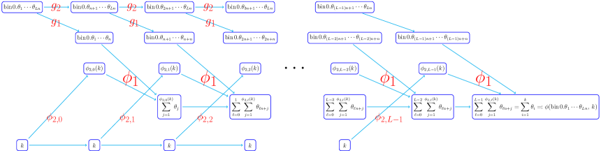
Figure 11: An illustration of the network implementing the desired function $\phi$ with the input $[\textnormal{bin}\hskip 1.2pt0.\theta_{1}\theta_{2}\cdots\theta_{Ln},k]^{T}$ for any $k\in\{1,2,\cdots,Ln\}$ and $\theta_{1},\theta_{2},\cdots,\theta_{Ln}\in\{0,1\}$. The network architecture is essentially determined by Equations (4.7), (4.8), (4.9), and (4.10), which are valid no matter what $\theta_{1},\theta_{2},\cdots,\theta_{Ln}\in\{0,1\}$ are. Thus, the desired function $\phi$ is independent of $\theta_{1},\theta_{2},\cdots,\theta_{Ln}\in\{0,1\}$. We omit ReLU ($\sigma$) for a neuron if its output is non-negative without ReLU.

By Lemma 4.3, we have

$$g_{1},g_{2}\in\textnormal{CPwL}(\mathbb{R},2^{n+1}-2)\subseteq\mathcal{NN}\big{(}\textnormal{\#input}=1;\ \textnormal{width\hskip 0.5ptvec}=[2^{n+1}-1];\ \textnormal{\#output}=1\big{)}.$$

Figure 12: An illustration of the network implementing the desired function $\phi_{2,\ell}$ for each $\ell\in\{0,1,\cdots,L-1\}$, based on $\min\{y,n\}=\tfrac{1}{2}\big{(}\sigma(y+n)-\sigma(-y-n)-\sigma(y-n)-\sigma(-y+n)\big{)}$.

Recall that $\phi_{1}\in\mathcal{NN}\big{(}\textnormal{width}\leq(n+1)2^{n+1};\ \textnormal{depth}\leq 3\big{)}$. As shown in Figure 12, $\phi_{2,\ell}(x)\in\mathcal{NN}(\textnormal{width}\leq 4;\ \textnormal{depth}\leq 2)$ for $\ell=0,1,\cdots,L-1$. Therefore, the network in Figure 11 has width

$$(2^{n+1}-1)\ +\ (2^{n+1}-1)\ +\ (n+1)2^{n+1}\ +\ 1\ +\ 4\ +\ 1=(n+3)2^{n+1}+4$$

and depth

$$2+L(1+3)=4L+2.$$

So we finish the proof. ∎

Next, we introduce Lemma 4.6 to map indices to the partial sum of given bits.

Lemma 4.6.

Given any $N,L\in\mathbb{N}^{+}$ and arbitrary $\theta_{m,k}\in\{0,1\}$ for $m=0,1,\cdots,M-1$ and $k=0,1,\cdots,Ln-1$, where $M=N^{2}L$ and $n=\lfloor\log_{3}(N+2)\rfloor$, there exists

$$\phi\in\mathcal{NN}\big{(}\textnormal{\#input}=2;\ \textnormal{width}\leq 6N+14;\ \textnormal{depth}\leq 5L+4;\ \textnormal{\#output}=1\big{)}$$

such that

$$\phi(m,k)=\sum_{j=0}^{k}\theta_{m,j},\quad\textnormal{ for $m=0,1,\cdots,M-1$\quad and\quad$k=0,1,\cdots,Ln-1$.}$$

Proof.

Define

$$y_{m}\coloneqq\textnormal{bin}\hskip 1.2pt0.\theta_{m,0}\theta_{m,1}\cdots\theta_{m,Ln-1},\quad\textnormal{for $m=0,1,\cdots,M-1$.}$$

Consider the sample set $\{(m,y_{m}):m=0,1,\cdots,M\}$, whose cardinality is

$$M+1=N\big{(}(NL-1)+1\big{)}+1.$$

By Lemma 4.1 (set $N_{1}=N$ and $N_{2}=NL-1$ therein), there exists

$$\begin{split}\phi_{1}&\in\mathcal{NN}(\textnormal{\#input}=1;\ \textnormal{width\hskip 0.5ptvec}=[2N,2(NL-1)+1];\ \textnormal{\#output}=1)\\ &=\mathcal{NN}(\textnormal{\#input}=1;\ \textnormal{width\hskip 0.5ptvec}=[2N,2NL-1];\ \textnormal{\#output}=1)\end{split}$$

such that

$$\phi_{1}(m)=y_{m},\quad\textnormal{for $m=0,1,\cdots,M-1$.}$$

By Lemma 4.5, there exists

$$\phi_{2}\in\mathcal{NN}\big{(}\textnormal{\#input}=2;\ \textnormal{width}\leq(n+3)2^{n+1}+4;\ \textnormal{depth}\leq 4L+2;\ \textnormal{\#output}=1\big{)}$$

such that, for any $\xi_{1},\xi_{2},\cdots,\xi_{Ln}\in\{0,1\}$, we have

$$\phi_{2}(\textnormal{bin}\hskip 1.2pt0.\xi_{1}\xi_{2}\cdots\xi_{Ln},\,k)=\sum_{j=1}^{k}\xi_{j},\quad\textnormal{for $k=1,2,\cdots,Ln$.}$$

It follows that, for any $\xi_{0},\xi_{1},\cdots,\xi_{Ln-1}\in\{0,1\}$, we have

$$\phi_{2}(\textnormal{bin}\hskip 1.2pt0.\xi_{0}\xi_{1}\cdots\xi_{Ln-1},\,k+1)=\sum_{j=0}^{k}\xi_{j},\quad\textnormal{for $k=0,1,\cdots,Ln-1$.}$$

Thus, for $m=0,1,\cdots,M-1$ and $k=0,1,\cdots,Ln-1$, we have

$$\phi_{2}(\phi_{1}(m),k+1)=\phi_{2}(y_{m},k+1)=\phi_{2}(0.\theta_{m,0}\theta_{m,1}\cdots\theta_{m,Ln-1},\,k+1)=\sum_{j=0}^{k}\theta_{m,j}.$$

Hence, the desired function $\phi$ can be implemented by the network shown in Figure 13. By Lemma 4.2, $\phi_{1}\in\mathcal{NN}(\textnormal{width\hskip 0.5ptvec}=[2N,2NL-1])\subseteq\mathcal{NN}(\textnormal{width}\leq 4N+2;\ \textnormal{depth}\leq L+1)$. It holds that

$$(n+3)2^{n+1}+4\leq 6\cdot(3^{n})+2=6\cdot(3^{\lfloor\log_{3}(N+2)\rfloor})+2\leq 6(N+2)+2=6N+14,$$

implying

$$\begin{split}\phi_{2}&\in\mathcal{NN}\big{(}\textnormal{\#input}=2;\ \textnormal{width}\leq(n+3)2^{n+1}+4;\ \textnormal{depth}\leq 4L+2;\ \textnormal{\#output}=1\big{)}\\ &\subseteq\mathcal{NN}\big{(}\textnormal{\#input}=2;\ \textnormal{width}\leq 6N+14;\ \textnormal{depth}\leq 4L+2;\ \textnormal{\#output}=1\big{)}.\end{split}$$

Therefore, the network in Figure 13 is with width $\max\{(4N+2)+1,6N+14\}=6N+14$ and depth $(4L+2)+1+(L+1)=5L+4$.

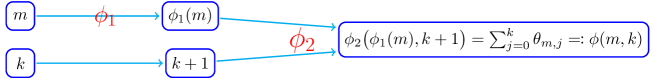
Figure 13: An illustration of the network implementing the desired function $\phi$ for $m=0,1,\cdots,M-1$ and $k=0,1,\cdots,Ln-1$.

So we finish the proof. ∎

Next, we apply Lemma 4.6 to prove Lemma 4.7 below, which is a key intermediate conclusion to prove Proposition 3.2.

Lemma 4.7.

For any $\varepsilon>0$ and $N,L\in\mathbb{N}^{+}$, denote $M=N^{2}L$ and $n=\lfloor\log_{3}(N+2)\rfloor$. Assume $y_{m,k}\geq 0$ for $m=0,1,\cdots,M-1\textnormal{ and }k=0,1,\cdots,Ln-1$ are samples with

$$|y_{m,k}-y_{m,k-1}|\leq\varepsilon,\quad\textnormal{for $m=0,1,\cdots,M-1\textnormal{\quad and\quad}k=1,2,\cdots,Ln-1$.}$$

Then there exists $\phi\in\mathcal{NN}(\textnormal{\#input}=2;\ \textnormal{width}\leq 16N+30;\ \textnormal{depth}\leq 5L+7;\ \textnormal{\#output}=1)$ such that

1. $|\phi(m,k)-y_{m,k}|\leq\varepsilon$ for $m=0,1,\cdots,M-1$ and $k=0,1,\cdots,Ln-1$;

2. $0\leq\phi(x_{1},x_{2})\leq\max\{y_{m,k}:m=0,1,\cdots,M-1\textnormal{\quad and\quad}k=0,1,\cdots,Ln-1\}$ for any $x_{1},x_{2}\in\mathbb{R}$.

Proof.

Define

$$a_{m,k}\coloneqq\lfloor y_{m,k}/\varepsilon\rfloor,\quad\textnormal{for $m=0,1,\cdots,M-1\textnormal{\quad and\quad}k=0,1,\cdots,Ln-1$.}$$

We will construct a function implemented by a ReLU network to map the index $(m,k)$ to $a_{m,k}\varepsilon$ for $m=0,1,\cdots,M-1\textnormal{ and }k=0,1,\cdots,Ln-1$.

Define $b_{m,0}\coloneqq 0$ and $b_{m,k}\coloneqq a_{m,k}-a_{m,k-1}$ for $m=0,1,\cdots,M-1\textnormal{ and }k=1,2,\cdots,Ln-1$. Since $|y_{m,k}-y_{m,k-1}|\leq\varepsilon$ for all $m$ and $k$, we have $b_{m,k}\in\{-1,0,1\}$. Hence, there exist $c_{m,k}\in\{0,1\}$ and $d_{m,k}\in\{0,1\}$ such that $b_{m,k}=c_{m,k}-d_{m,k}$, which implies

$$\begin{split}a_{m,k}=a_{m,0}+\sum_{i=1}^{k}(a_{m,i}-a_{m,i-1})&=a_{m,0}+\sum_{i=1}^{k}b_{m,i}=a_{m,0}+\sum_{i=0}^{k}b_{m,i}\\ &=a_{m,0}+\sum_{i=0}^{k}c_{m,i}-\sum_{i=0}^{k}d_{m,i},\end{split}$$

for $m=0,1,\cdots,M-1\textnormal{ and }k=0,1,\cdots,Ln-1$.

Consider the sample set

$$\big{\{}(m,a_{m,0}):m=0,1,\cdots,M-1\big{\}}\bigcup\{(M,0)\}.$$

Its size is $M+1=N\cdot\big{(}(NL-1)+1\big{)}+1$, by Lemma 4.1 (set $N_{1}=N$ and $N_{2}=NL-1$ therein), there exists

$$\psi_{1}\in\mathcal{NN}(\textnormal{width\hskip 0.5ptvec}=[2N,2(NL-1)+1])=\mathcal{NN}(\textnormal{width\hskip 0.5ptvec}=[2N,2NL-1])$$

such that

$$\psi_{1}(m)=a_{m,0},\quad\textnormal{for $m=0,1,\cdots,M-1$.}$$

By Lemma 4.6, there exist $\psi_{2},\psi_{3}\in\mathcal{NN}(\textnormal{width}\leq 6N+14;\ \textnormal{depth}\leq 5L+4)$ such that

$$\psi_{2}(m,k)=\sum\limits_{i=0}^{k}c_{m,i}\quad\textnormal{and}\quad\psi_{3}(m,k)=\sum\limits_{i=0}^{k}d_{m,i},$$

for $m=0,1,\cdots,M-1\textnormal{ and }k=0,1,\cdots,Ln-1$. Hence, it holds that

$$a_{m,k}=a_{m,0}+\sum_{i=0}^{k}c_{m,i}-\sum_{i=0}^{k}d_{m,i}=\psi_{1}(m)+\psi_{2}(m,k)-\psi_{3}(m,k),$$ (4.11)

for $m=0,1,\cdots,M-1\textnormal{ and }k=0,1,\cdots,Ln-1$.

Define

$$y_{\textnormal{max}}\coloneqq\max\{y_{m,k}:m=0,1,\cdots,M-1\textnormal{\quad and\quad}k=0,1,\cdots,Ln-1\}.$$

Then the desired function can be implemented by two sub-networks shown in Figure 14.

(a) $\phi_{1}$

(b) $\phi_{2}$

Figure 14: Illustrations of two sub-networks implementing the desired function $\phi=\phi_{2}\circ\phi_{1}$ for $m=0,1,\cdots,M-1$ and $k=0,1,\cdots,Ln-1$, based on Equation (4.11) and the fact $\min\{x_{1},x_{2}\}=\tfrac{x_{1}+x_{2}-|x_{1}-x_{2}|}{2}=\tfrac{\sigma(x_{1}+x_{2})-\sigma(-x_{1}-x_{2})-\sigma(x_{1}-x_{2})-\sigma(-x_{1}+x_{2})}{2}$.

By Lemma 4.2,

$$\begin{split}\psi_{1}&\in\mathcal{NN}(\textnormal{\#input}=1;\ \textnormal{width\hskip 0.5ptvec}=[2N,2NL-1];\ \textnormal{\#output}=1)\\ &\subseteq\mathcal{NN}(\textnormal{\#input}=1;\ \textnormal{width}\leq 4N+2;\ \textnormal{depth}\leq L+1;\ \textnormal{\#output}=1).\end{split}$$

Recall that $\psi_{2},\psi_{3}\in\mathcal{NN}(\textnormal{width}\leq 6N+14;\ \textnormal{depth}\leq 5L+4)$. Thus, $\phi_{1}\in\mathcal{NN}(\textnormal{width}\leq(4N+2)+2(6N+14)=16N+30;\ \textnormal{depth}\leq(5L+4)+1=5L+5)$ as shown in Figure 14. And it is clear that $\phi_{2}\in\mathcal{NN}(\textnormal{width}\leq 4;\ \textnormal{depth}\leq 2)$, implying $\phi=\phi_{2}\circ\phi_{1}\in\mathcal{NN}(\textnormal{width}\leq 16N+30;\ \textnormal{depth}\leq(5L+5)+2=5L+7)$.

Clearly, $0\leq\phi(x_{1},x_{2})\leq y_{\textnormal{max}}$ for any $x_{1},x_{2}\in\mathbb{R}$, since $\phi(x_{1},x_{2})=\phi_{2}\circ\phi_{1}(x_{1},x_{2})=\max\{\sigma(\phi_{1}(x_{1},x_{2})),y_{\textnormal{max}}\}$.

Note that $0\leq a_{m,k}\varepsilon=\lfloor y_{m,k}/\varepsilon\rfloor\varepsilon\leq y_{\textnormal{max}}$. Then we have $\phi(m,k)=\phi_{2}\circ\phi_{1}(m,k)=\phi_{2}(a_{m,k}\varepsilon)=\max\{\sigma(a_{m,k}\varepsilon),y_{\textnormal{max}}\}=a_{m,k}\varepsilon$. Therefore,

$$\begin{split}|\phi(m,k)-y_{m,k}|=\left|a_{m,k}\varepsilon-y_{m,k}\right|=\big{|}\lfloor y_{m,k}/\varepsilon\rfloor\varepsilon-y_{m,k}\big{|}\leq\varepsilon,\end{split}$$

for $m=0,1,\cdots,M-1$ and $k=0,1,\cdots,Ln-1$. Hence, we finish the proof. ∎

Finally, we apply Lemma 4.7 to prove Proposition 3.2.

Proof of Proposition 3.2.

Denote $M=N^{2}L$, $n=\lfloor\log_{3}(N+2)\rfloor$, and ${\widehat{L}}=Ln$. We may assume $J=MLn=M{\widehat{L}}$ since we can set $y_{J-1}=y_{J}=y_{J+1}=\cdots=y_{M{\widehat{L}}-1}$ if $J<M{\widehat{L}}$.

Consider the sample set

$$\big{\{}(m{\widehat{L}},m):m=0,1,\cdots,M\big{\}}\bigcup\big{\{}(m{\widehat{L}}+{\widehat{L}}-1,m):m=0,1,\cdots,M-1\big{\}}.$$

Its size is $2M+1=N\cdot\big{(}(2NL-1)+1\big{)}+1$. By Lemma 4.1 (set $N_{1}=N$ and $N_{2}=NL-1$ therein), there exists

$$\phi_{1}\in\mathcal{NN}(\textnormal{width\hskip 0.5ptvec}=[2N,2(2NL-1)+1])=\mathcal{NN}(\textnormal{width\hskip 0.5ptvec}=[2N,4NL-1])$$

such that

• $\phi_{1}(M{\widehat{L}})=M$ and $\phi_{1}(m{\widehat{L}})=\phi_{1}(m{\widehat{L}}+{\widehat{L}}-1)=m$ for $m=0,1,\cdots,M-1$.

• $\phi_{1}$ is linear on each interval $[m{\widehat{L}},m{\widehat{L}}+{\widehat{L}}-1]$ for $m=0,1,\cdots,M-1$.

It follows that

$$\phi_{1}(j)=m,\quad\textnormal{and}\quad j-{\widehat{L}}\phi_{1}(j)=k,\quad\textnormal{where $j=m{\widehat{L}}+k$},$$ (4.12)

for $m=0,1,\cdots,M-1$ and $k=0,1,\cdots,{\widehat{L}}-1$.

Since $J=M{\widehat{L}}$, any $j\in\{0,1,\cdots,J-1\}$ can be uniquely indexed as $j=m{\widehat{L}}+k$ for $m\in\{0,1,\cdots,M-1\}$ and $k\in\{0,1,\cdots,{\widehat{L}}-1\}$. So we can denote $y_{j}=y_{m{\widehat{L}}+k}$ as $y_{m,k}$. Then by Lemma 4.7, there exists $\phi_{2}\in\mathcal{NN}(\textnormal{width}\leq 16N+30;\ \textnormal{depth}\leq 5L+7)$ such that

$$|\phi_{2}(m,k)-y_{m,k}|\leq\varepsilon,\quad\textnormal{for $m=0,1,\cdots,M-1\textnormal{\quad and\quad}k=0,1,\cdots,{\widehat{L}}-1$},$$ (4.13)

and

$$0\leq\phi_{2}(x_{1},x_{2})\leq y_{\textnormal{max}},\quad\textnormal{for any $x_{1},x_{2}\in\mathbb{R}$,}$$ (4.14)

where $y_{\textnormal{max}}\coloneqq\max\{y_{m,k}:m=0,1,\cdots,M-1\textnormal{ and }k=0,1,\cdots,{\widehat{L}}-1\}=\max\{y_{j}:j=0,1,\cdots,J-1\}$.

Figure 15: An illustration of the ReLU network implementing the desired function $\phi$ based Equation (4.12). The index $j\in\{0,1,\cdots,M{\widehat{L}}-1\}$ is unique represented by $j=mL+k$ for $m\in\{0,1,\cdots,M-1\}$ and $k\in\{0,1,\cdots,{\widehat{L}}-1\}$.

By Lemma 4.2,

$$\begin{split}\phi_{1}&\in\mathcal{NN}(\textnormal{\#input}=1;\ \textnormal{width\hskip 0.5ptvec}=[2N,4NL-1];\ \textnormal{\#output}=1)\\ &\subseteq\mathcal{NN}(\textnormal{\#input}=1;\ \textnormal{width}\leq 8N+2;\textnormal{depth}\leq L+1;\ \textnormal{\#output}=1).\end{split}$$

Recall that $\phi_{2}\in\mathcal{NN}(\textnormal{width}\leq 16N+30;\ \textnormal{depth}\leq 5L+7)$. So $\phi\in\mathcal{NN}(\textnormal{width}\leq 16N+30;\ \textnormal{depth}\leq(L+1)+2+(5L+7)=6L+10)$ as shown in Figure 15.

Equation (4.14) implies

$$0\leq\phi(x)\leq y_{\textnormal{max}},\quad\textnormal{for any $x\in\mathbb{R}$,}$$

since $\phi$ is given by $\phi(x)=\phi_{2}\big{(}\phi_{1}(x),x-{\widehat{L}}\phi_{1}(x)\big{)}$.

Represent $j\in\{0,1,\cdots,M{\widehat{L}}-1\}$ via $j=m{\widehat{L}}+k$ for $m=0,1,\cdots,M-1$ and $k=0,1,\cdots,{\widehat{L}}-1$. Then, by Equation (4.13), we have

$$\begin{split}|\phi(j)-y_{j}|=|\phi_{2}\big{(}\phi_{1}(j),j-{\widehat{L}}\phi_{1}(j)\big{)}-y_{j}|=|\phi_{2}(m,k)-y_{m,k}|\leq\varepsilon,\end{split}$$

for any $j\in\{0,1,\cdots,M{\widehat{L}}-1\}=\{0,1,\cdots,J-1\}$. So we finish the proof. ∎

We would like to remark that the key idea in the proof of Proposition 3.2 is the bit extraction technique in Lemma 4.5, which allows us to store $Ln$ bits in a binary number $\textnormal{bin}\hskip 1.2pt0.\theta_{1}\theta_{2}\cdots\theta_{Ln}$ and extract each bit $\theta_{i}$. The extraction operator can be efficiently carried out via a deep ReLU neural network demonstrating the power of depth.

5 Conclusion and future work

This paper aims at a quantitative and optimal approximation rate for ReLU networks in terms of the width and depth to approximate continuous functions. It is shown by construction that ReLU networks with width ${\mathcal{O}}(N)$ and depth ${\mathcal{O}}(L)$ can approximate an arbitrary continuous function $f$ on $[0,1]^{d}$ with an approximation rate ${\mathcal{O}}\big{(}\,\omega_{f}\big{(}(N^{2}L^{2}\ln N)^{-1/d}\big{)}\,\big{)}$. By connecting the approximation property to VC-dimension, we prove that such a rate is optimal for Hölder continuous functions on $[0,1]^{d}$ in terms of the width and depth separately, and hence this rate is also optimal for the whole continuous function class. We also extend our analysis to general continuous functions on any bounded subset of $\mathbb{R}^{d}$. We would like to remark that our analysis was based on the fully connected feed-forward neural networks and the ReLU activation function. It would be very interesting to extend our conclusions to neural networks with other types of architectures (e.g., convolutional neural networks) and activation functions (e.g., tanh and sigmoid functions).

References

- [1] M. Anthony and P. L. Bartlett, Neural Network Learning: Theoretical Foundations, Cambridge University Press, New York, NY, USA, 1st ed., 2009.
- [2] A. R. Barron, Universal approximation bounds for superpositions of a sigmoidal function, IEEE Transactions on Information Theory, 39 (1993), pp. 930–945.
- [3] P. Bartlett, V. Maiorov, and R. Meir, Almost linear VC-dimension bounds for piecewise polynomial networks, Neural Computation, 10 (1998), pp. 2159–2173.
- [4] M. Bianchini and F. Scarselli, On the complexity of neural network classifiers: A comparison between shallow and deep architectures, IEEE Transactions on Neural Networks and Learning Systems, 25 (2014), pp. 1553–1565.
- [5] L. Chen and C. Wu, A note on the expressive power of deep rectified linear unit networks in high-dimensional spaces, Mathematical Methods in the Applied Sciences, 42 (2019), pp. 3400–3404.
- [6] G. Cybenko, Approximation by superpositions of a sigmoidal function, MCSS, 2 (1989), pp. 303–314.
- [7] W. E, C. Ma, and Q. Wang, A priori estimates of the population risk for residual networks, arXiv e-prints, (2019).
- [8] W. E, C. Ma, and L. Wu, A priori estimates of the population risk for two-layer neural networks, Communications in Mathematical Sciences, 17 (2019), pp. 1407–1425.
- [9] W. E and Q. Wang, Exponential convergence of the deep neural network approximation for analytic functions, CoRR, abs/1807.00297 (2018).
- [10] W. E and S. Wojtowytsch, On the banach spaces associated with multi-layer ReLU networks: Function representation, approximation theory and gradient descent dynamics, arXiv e-prints, (2020).
- [11] , A priori estimates for classification problems using neural networks, arXiv e-prints, (2020).
- [12] , Representation formulas and pointwise properties for barron functions, arXiv e-prints, (2020).
- [13] N. Harvey, C. Liaw, and A. Mehrabian, Nearly-tight VC-dimension bounds for piecewise linear neural networks, in Proceedings of the 2017 Conference on Learning Theory, S. Kale and O. Shamir, eds., vol. 65 of Proceedings of Machine Learning Research, Amsterdam, Netherlands, 07–10 Jul 2017, PMLR, pp. 1064–1068.
- [14] J. He, X. Jia, J. Xu, L. Zhang, and L. Zhao, Make regularization effective in training sparse CNN, Computational Optimization and Applications, 77 (2020), pp. 163–182.
- [15] K. Hornik, Approximation capabilities of multilayer feedforward networks, Neural Networks, 4 (1991), pp. 251–257.
- [16] K. Hornik, M. Stinchcombe, and H. White, Multilayer feedforward networks are universal approximators, Neural Networks, 2 (1989), pp. 359–366.
- [17] K. Kawaguchi, Deep learning without poor local minima, in Advances in Neural Information Processing Systems 29, D. D. Lee, M. Sugiyama, U. V. Luxburg, I. Guyon, and R. Garnett, eds., Curran Associates, Inc., 2016, pp. 586–594.
- [18] K. Kawaguchi and Y. Bengio, Depth with nonlinearity creates no bad local minima in resnets, Neural Networks, 118 (2019), pp. 167–174.
- [19] M. J. Kearns and R. E. Schapire, Efficient distribution-free learning of probabilistic concepts, Journal of Computer and System Sciences, 48 (1994), pp. 464–497.
- [20] Q. Li, T. Lin, and Z. Shen, Deep learning via dynamical systems: An approximation perspective, Journal of European Mathematical Society, (to appear).
- [21] Q. Li, C. Tai, and W. E, Stochastic modified equations and dynamics of stochastic gradient algorithms I: Mathematical foundations, Journal of Machine Learning Research, 20 (2019), pp. 1–47.
- [22] S. Liang and R. Srikant, Why deep neural networks?, CoRR, abs/1610.04161 (2016).
- [23] H. Lin and S. Jegelka, Resnet with one-neuron hidden layers is a universal approximator, in Advances in Neural Information Processing Systems, S. Bengio, H. Wallach, H. Larochelle, K. Grauman, N. Cesa-Bianchi, and R. Garnett, eds., vol. 31, Curran Associates, Inc., 2018.
- [24] J. Lu, Z. Shen, H. Yang, and S. Zhang, Deep network approximation for smooth functions, arXiv e-prints, (2020).
- [25] Z. Lu, H. Pu, F. Wang, Z. Hu, and L. Wang, The expressive power of neural networks: A view from the width, in Advances in Neural Information Processing Systems 30, I. Guyon, U. V. Luxburg, S. Bengio, H. Wallach, R. Fergus, S. Vishwanathan, and R. Garnett, eds., Curran Associates, Inc., 2017, pp. 6231–6239.
- [26] H. Montanelli, H. Yang, and Q. Du, Deep ReLU networks overcome the curse of dimensionality for bandlimited functions, Journal of Computational Mathematics, (to appear).
- [27] G. F. Montufar, R. Pascanu, K. Cho, and Y. Bengio, On the number of linear regions of deep neural networks, in Advances in Neural Information Processing Systems 27, Z. Ghahramani, M. Welling, C. Cortes, N. D. Lawrence, and K. Q. Weinberger, eds., Curran Associates, Inc., 2014, pp. 2924–2932.
- [28] B. Neyshabur, Z. Li, S. Bhojanapalli, Y. LeCun, and N. Srebro, The role of over-parametrization in generalization of neural networks, in International Conference on Learning Representations, 2019.
- [29] Q. N. Nguyen and M. Hein, The loss surface of deep and wide neural networks, CoRR, abs/1704.08045 (2017).
- [30] P. Petersen and F. Voigtlaender, Optimal approximation of piecewise smooth functions using deep ReLU neural networks, Neural Networks, 108 (2018), pp. 296–330.
- [31] A. Sakurai, Tight bounds for the VC-dimension of piecewise polynomial networks, in Advances in Neural Information Processing Systems, Neural information processing systems foundation, 1999, pp. 323–329.
- [32] Z. Shen, H. Yang, and S. Zhang, Nonlinear approximation via compositions, Neural Networks, 119 (2019), pp. 74–84.
- [33] , Deep network approximation characterized by number of neurons, Communications in Computational Physics, 28 (2020), pp. 1768–1811.
- [34] , Deep network with approximation error being reciprocal of width to power of square root of depth, Neural Computation, 33 (2021), pp. 1005–1036.
- [35] , Neural network approximation: Three hidden layers are enough, Neural Networks, 141 (2021), pp. 160–173.
- [36] J. W. Siegel and J. Xu, Approximation rates for neural networks with general activation functions, Neural Networks, 128 (2020), pp. 313–321.
- [37] , Optimal approximation rates and metric entropy of ReLUk and cosine networks, arXiv e-prints, (2021).
- [38] P. Urysohn, Über die Mächtigkeit der zusammenhängenden Mengen, Mathematische Annalen, 94 (1925), pp. 262–295.
- [39] H. Whitney, Analytic extensions of differentiable functions defined in closed sets, Transactions of the American Mathematical Society, 36 (1934), pp. 63–89.
- [40] D. Yarotsky, Error bounds for approximations with deep ReLU networks, Neural Networks, 94 (2017), pp. 103–114.
- [41] , Optimal approximation of continuous functions by very deep ReLU networks, in Proceedings of the 31st Conference On Learning Theory, S. Bubeck, V. Perchet, and P. Rigollet, eds., vol. 75 of Proceedings of Machine Learning Research, PMLR, 06–09 Jul 2018, pp. 639–649.
- [42] , Elementary superexpressive activations, arXiv e-prints, (2021).
- [43] D. Yarotsky and A. Zhevnerchuk, The phase diagram of approximation rates for deep neural networks, in Advances in Neural Information Processing Systems, H. Larochelle, M. Ranzato, R. Hadsell, M. F. Balcan, and H. Lin, eds., vol. 33, Curran Associates, Inc., 2020, pp. 13005–13015.
- [44] S. Zhang, Deep neural network approximation via function compositions, PhD Thesis, National University of Singapore, (2020). URL https://scholarbank.nus.edu.sg/handle/10635/186064.