Peridynamic stress is a weighted static Virial stress

Abstract

The peridynamic stress tensor proposed by Lehoucq and Silling [1] is cumbersome to implement in numerical computations. In this note, we show that the peridynamic stress tensor has the mathematical expression of a weighted static Virial stress derived by Irving and Kirkwood [2], which offers a simple and clear expression for numerical calculations of peridynamic stress tensor.

Peridynamics is reformulation of non-local continuum mechanics or computational non-local mechanics [3, 4]. In the peridynamic equation of motion, following the notation of Silling and Lehoucq [4] one can write the balance of linear momentum as

$$\rho\ddot{\bf u}({\bf X},t)=\int_{\mathcal{H}_{X}}{\bf f}({\bf X}^{\prime},{\bf X},t)dV_{X^{\prime}}+{\bf b}({\bf X},t),~{}~{}\forall{\bf X}\in\mathcal{B}$$ (1)

where $\mathcal{B}\subset^{3}$; $\mathcal{H}_{X}\subset\mathcal{B}$ is a the horizon of the material point ${\bf X}$; $\rho$ is the material density, and ${\bf b}({\bf X},t)$ is the body force. The term

$$\int_{\mathcal{H}_{X}}{\bf f}({\bf X}^{\prime},{\bf X},t)dV_{X^{\prime}}$$

replaces the divergence of the first Piola-Kirchhoff stress $\nabla\cdot{\bf P}$ at the material point ${\bf X}$.

By definition,

$${\bf f}({\bf X}^{\prime},{\bf X},t):=\bigl{(}{\bf t}({\bf X}^{\prime},{\bf X},t)-{\bf t}({\bf X},{\bf X}^{\prime},t)\bigr{)}=-{\bf f}({\bf X},{\bf X}^{\prime},t)$$ (2)

is antisymmetric, where ${\bf X},{\bf X}^{\prime}$ are the position vectors of material points in the referential configuration.

Equation (1) extends the balance equation of linear momentum to nonlocal media. However, it loses some valuable properties that are associated with the local balance law such as the divergence theorem or the Gauss theorem.

Noticing such inadequacy, Lehoucq and Silling [1] define the following nonlocal Peridynamic Stress tensor

$${\bm{\varsigma}}({\bf X}):={1\over 2}\int_{\mathcal{S}^{2}}\int_{0}^{\infty}\int_{0}^{\infty}(y+z)^{2}{\bf f}({\bf X}+y{\bf M},{\bf X}-z{\bf M})\otimes{\bf M}dzdyd\Omega_{M}~{},$$ (3)

where $\mathcal{S}^{2}$ is the unit sphere. By doing so, we have the relation

$$\nabla\cdot{\bm{\varsigma}}=\int_{\mathcal{H}_{X}}{\bf f}({\bf X}^{\prime},{\bf X},t)dV_{X^{\prime}}~{}.$$ (4)

where $\nabla$ is the local gradient operator. An immediate benefit of Eq. (3) is that we can link the divergence of the peridynamic stress with the boundary linear momentum flux, i.e.

$$\int_{\mathcal{B}}\nabla\cdot{\bm{\varsigma}}dV_{X}=\int_{\partial\mathcal{B}}{\bm{\varsigma}}\cdot{\bf N}dS_{X}~{},$$

which allows us to establish peridynamics-based Galerkin weak formulations conveniently, and maybe even formulate peridynamics theories of plates and shells.

By using Noll’s lemmas [5], such nonlocal integral theorems have been late extended to a more general situations by Gunzburger and Lehoucq [6] and Du et. al. [7]. However, in practice the peridynamic stress defined in Eq. (3) is cumbersome to evaluate. To resolve this issue, in this note, we show that in peridynamic particle formulation, which is a special case of the non-local continuum, the peridynamic stress tensor has the exact expression of the static Virial stress defined by Irving and Kirkwood [2].

Theorem 0.1 (Alternative form of Peridynamic Stress tensor).

Consider the peridynamics force density that can be expressed as the following expression of the Irving-Kirkwoods formulation [2, 4],

$${\bf f}({\bf X}^{\prime},{\bf X},t)=\sum_{I=1}^{N_{X}}\sum_{J=1}^{N_{X}}{\bf F}_{IJ}\delta({\bf X}-{\bf X}_{I})\delta({\bf X}^{\prime}-{\bf X}_{J})$$ (5)

where ${\bf F}_{IJ}$ is the force acting on the particle $I$ from the particle $J$ (see Fig. 1); $N_{X}$ is the total number of particles inside the horizon $\mathcal{H}_{X}$. The nonlocal peridynamic stress

$${\bm{\varsigma}}({\bf X}):={1\over 2}\int_{\mathcal{S}^{2}}\int_{0}^{\infty}\int_{0}^{\infty}(y+z)^{2}{\bf f}({\bf X}+y{\bf M},{\bf X}-z{\bf M})\otimes{\bf M}dzdyd\Omega_{M}~{},$$ (6)

has the following exact form,

$${\bm{\varsigma}}({\bf X}):=-{1\over 2}\sum_{I=1}^{N_{X}}\sum_{J=1}^{N_{X}}{\bf F}_{IJ}\otimes{({\bf X}_{I}-{\bf X})\over|{\bf X}_{I}-{\bf X}|}|{\bf X}_{I}-{\bf X}_{J}|,~{}~{}{\bf X}_{J},{\bf X}_{I}\in\mathcal{H}_{X},~{}~{}{\bf X}_{J}\not={\bf X}_{I}~{}.$$ (7)

where ${\bf F}_{IJ}$ is the force acting on the atom $I$ by the atom $J$.

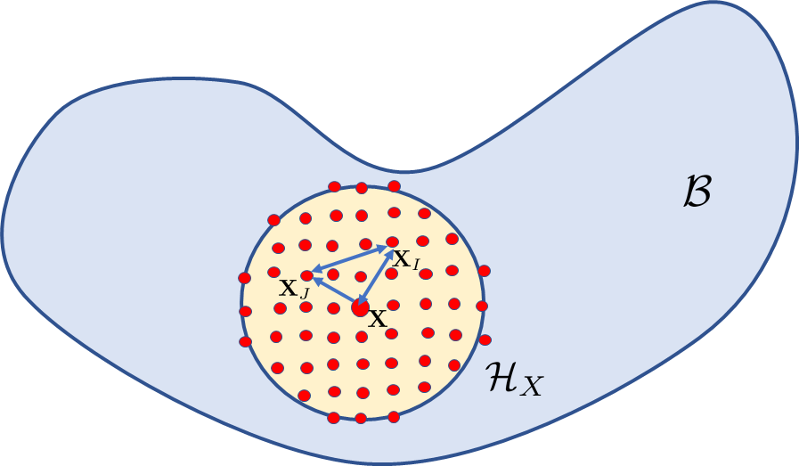
Figure 1: Illustration of peridynamics particle sampling strategy

Proof.

 
Based on Noll’s lemma [5], we can write the first peridynamics Piola-Kirchhoff stress as

$${\bm{\varsigma}}({\bf X}) = {1\over 2}\int_{S^{2}}d\Omega_{m}\int_{0}^{\infty}R^{2}dR\int_{0}^{1}{\bf f}({\bf X}+\alpha R{\bf M},{\bf X}-(1-\alpha)R{\bf M})\otimes{\bf M}d\alpha$$ (8)

$$= -{1\over 2}\int_{{}^{3}}dV_{R}\int_{0}^{1}{\bf f}({\bf X}+\alpha{\bf R},{\bf X}-(1-\alpha){\bf R})\otimes{\bf R}d\alpha~{},~{}\forall{\bf X}\in\mathcal{B}$$

Considering the Irving-Kirkwood formalism [2], we have the following peridynamics sampling formulation (see Fig. 1)

$${\bf f}({\bf X}^{\prime},{\bf X})=-{\bf f}({\bf X},{\bf X}^{\prime})=-\sum_{J=1}^{N}{\bf F}_{IJ}\delta({\bf X}-{\bf X}_{I})\delta({\bf X}^{\prime}-{\bf X}_{J}),~{}~{}{\bf X}_{I}\not={\bf X}_{J}~{}.$$ (9)

Letting

$${\bf X}={\bf X}_{C}+\alpha{\bf R},~{}{\rm and}~{}~{}{\bf X}^{\prime}={\bf X}_{C}-(1-\alpha){\bf R}$$

and substituting them into Eq. (9), we then have

$${\bf f}({\bf X}+\alpha{\bf R},{\bf X}-(1-\alpha){\bf R})$$ (10)

$$= \sum_{I=1}^{N_{X}}\sum_{J=1}^{N_{X}}{\bf F}_{IJ}\delta(\alpha{\bf R}-({\bf X}_{I}-{\bf X}_{C}))\delta(\alpha{\bf R}-{\bf R}-({\bf X}_{J}-{\bf X}_{C})).$$

where ${\bf X}_{I},{\bf X}_{J}\in\mathcal{H}_{X_{C}},~{}~{}{\bf X}_{I}\not={\bf X}_{J}$.

Considering the following integration identities

$$\delta(g(x))={\delta(x-x_{0})\over|g^{\prime}(x_{0})|}$$ (11)

$$\int_{-\infty}^{\infty}\delta(\xi-x)\delta(x-\eta)dx=\delta(\eta-\xi)$$ (12)

we have

$$\int_{{}^{3}}\delta(\alpha{\bf R}-({\bf X}_{I}-{\bf X}_{C}))\delta(\alpha{\bf R}-{\bf R}-({\bf X}_{J}-{\bf X}_{C})){\bf R}d(\alpha V_{R})$$

$$=\alpha^{-1}({\bf X}_{I}-{\bf X}_{C})\delta(({\bf X}_{I}-{\bf X}_{J})-\alpha^{-1}({\bf X}_{I}-{\bf X}_{C}))~{}.$$ (13)

Let $\xi=\alpha^{-1}$ and $d\xi=-{\xi\over\alpha}d\alpha\to d\alpha=-\xi^{-2}d\xi$. We then can have,

$${\bm{\varsigma}}({\bf X}_{C}) = -{1\over 2}\bigl{(}\sum_{I=1}^{N_{X}}\sum_{J=1}^{N_{X}}{\bf F}_{IJ}\bigr{)}\otimes({\bf X}_{I}-{\bf X}_{C})$$ (14)

$$\cdot\int_{0}^{\infty}\delta(({\bf X}_{I}-{\bf X}_{J})-\xi({\bf X}_{I}-{\bf X}_{C}))\xi^{-1}d\xi$$

$$= -{1\over 2}\sum_{I=1}^{N_{X}}\sum_{J=1}^{N_{X}}{\bf F}_{IJ}\otimes\Bigl{(}{{\bf X}_{I}-{\bf X}_{C}\over|{\bf X}_{I}-{\bf X}_{C}|}\Bigr{)}|{\bf X}_{I}-{\bf X}_{J}|$$

Let ${\bf X}_{C}\to{\bf X}$. We prove the claim. ∎

Remark 0.1.

The above expression may be rewritten as

$${\bm{\varsigma}}({\bf X}) = -{1\over 2}\sum_{I=1}^{N_{X}}\sum_{J=1}^{N_{X}}{\bf F}_{IJ}\otimes({\bf X}_{I}-{\bf X}_{J})\Bigl{(}{|{\bf X}_{I}-{\bf X}_{J}|\over{\bf X}_{I}-{\bf X}_{J}}\Bigr{)}\cdot\Bigl{(}{{\bf X}_{I}-{\bf X}\over|{\bf X}_{I}-{\bf X}|}\Bigr{)}~{}.$$ (15)

which is a weighted static Virial stress.

For the state-based peridynamics, we have the following result.

Corollary 0.1.1 (Peridynamics PK-I stress tensor).

For continuous variable ${\bf X}_{i},{\bf X}_{j}\in\mathcal{H}_{C}$, we let

$${\bf f}({\bf X}_{i},{\bf X}_{j})=w(X_{ij})\Bigl{(}{\bf P}_{j}{\bf K}_{j}{\bf X}_{ij}-{\bf P}_{i}{\bf K}_{i}{\bf X}_{ji}\Bigr{)}$$ (16)

where ${\bf K}_{i}={\bf K}({\bf K}_{i})$ is the shape tensor; $w(X_{ij}=w(|{\bf X}_{j}-{\bf X}_{i}|)$ is a window function; ${\bf X}_{ij}={\bf X}_{j}-{\bf X}_{i}$, and ${\bf P}({\bf X}_{i})$ is the first Piola-Kirchhoff stress at the local continuum material point ${\bf X}_{i}$ . For the first Piola-Kirchhoff stress tensor, ${\bf P}({\bf X}),~{}{\bf X}\in\Omega_{0}$, the nonlocal divergence of ${\bf P}$,

$$\mathfrak{D}[{\bf P}]=\int_{\Omega_{0}}w(X_{ij})\Bigl{(}{\bf P}_{j}{\bf X}_{ij}-{\bf P}_{i}{\bf X}_{ji}\Bigr{)}\cdot{\bf K}^{-1}dV_{j},~{}~{}\forall{\bf X}_{i}\in\Omega_{0},$$ (17)

equals to the local divergence of a nonlocal counterpart, $\widetilde{\bf P}$,

$$\nabla\cdot\widetilde{\bf P}=\mathfrak{D}[{\bf P}]$$ (18)

where

$$\widetilde{\bf P}({\bf X}) := {1\over 2}\sum_{I=1}^{N_{X}}\sum_{J=1,J\not=I}^{N_{X}}{\bf f}({\bf X}_{I},{\bf X}_{J})\otimes({\bf X}_{I}-{\bf X}_{J})\Bigl{(}{|{\bf X}_{I}-{\bf X}_{J}|\over({\bf X}_{I}-{\bf X}_{J})}{|{\bf X}_{I}-{\bf X}|\over({\bf X}_{I}-{\bf X})},~{}~{}$$ (19)

$$\forall~{}{\bf X}\in\mathcal{B},~{}~{}{\bf X}_{I},{\bf X}_{J}\in\mathcal{H}_{X}~{}.$$

Remark 0.2.

Note that the above result does not restricted to peridynamics PK-I stress tensor, and it is valid for general peridynamics stress tensor after small modifications depending on the case that is under consideration. Amazingly, the result reveals that fact that the mesoscale peridynamic stress tensor has exactly the same expression as that of the microscale static Virial stress, except that it does not count for the contribution from the kinetic energy. Moreover, the expression (7) is so simple that it can be readily implemented in numerical calculations without much trouble.

Reference

References

[1]
R.B. Lehoucq and S.A. Silling.
Force flux and the peridynamic stress tensor.
Journal of the Mechanics and Physics of Solids,
56(4):1566–1577, 2008.
[2]
J.H. Irving and J.G. Kirkwood.
The statistical mechanical theory of transport processes. iv. the
equations of hydrodynamics.
The Journal of Chemical Physics, 18(6):817–829, 1950.
[3]
S.A. Silling.
Reformulation of elasticity theory for discontinuities and long-range
forces.
Journal of the Mechanics and Physics of Solids, 48(1):175–209,
2000.
[4]
S.A. Silling and R.B. Lehoucq.
Peridynamic theory of solid mechanics.
Advances in Applied Mechanics, pages 73–168, 2010.
[5]
W. Noll.
Die herleitung der grundgleichungen der thermomechanik der kontinua
aus der statistischen mechanik.
Journal of Rational Mechanics and Analysis, 4:627–646, 1955.
[6]
M. Gunzburger and R.B. Lehoucq.
A nonlocal vector calculus with application to nonlocal boundary
value problems.
Multiscale Modeling & Simulation, 8(5):1581–1598, 2010.
[7]
Q. Du, M. Gunzburger, R.B. Lehoucq, and K. Zhou.
A nonlocal vector calculus, nonlocal volume-constrained problems, and
nonlocal balance laws.
Mathematical Models and Methods in Applied Sciences,
23(03):493–540, 2013.