Smeariness Begets Finite Sample Smeariness

Abstract

Fréchet means are indispensable for nonparametric statistics on non-Euclidean spaces. For suitable random variables, in some sense, they “sense” topological and geometric structure. In particular, smeariness seems to indicate the presence of positive curvature. While smeariness may be considered more as an academical curiosity, occurring rarely, it has been recently demonstrated that finite sample smeariness (FSS) occurs regularly on circles, tori and spheres and affects a large class of typical probability distributions. FSS can be well described by the modulation measuring the quotient of rescaled expected sample mean variance and population variance. Under FSS it is larger than one – that is its value on Euclidean spaces – and this makes quantile based tests using tangent space approximations inapplicable. We show here that near smeary probability distributions there are always FSS probability distributions and as a first step towards the conjecture that all compact spaces feature smeary distributions, we establish directional smeariness under curvature bounds.

1 Introduction

For nonparametric statistics of manifold data, the Fréchet mean plays a central role, both in descriptive and inferential statistics. For quite some while it was assumed that its asymptotics can be approximated under very general conditions by that of means of data projected to a suitable tangent space, e.g Hendriks and Landsman (1998); Bhattacharya and Patrangenaru (2005); Huckemann (2011a, b); Bhattacharya and Lin (2017). Under existence of second moments, these follow a classical central limit theorem. In the last decade, however, other asymptotic regimes have been discovered, yielding so called smeary limiting rates, limiting rates that are slower than the classical $n^{-1/2}$, where $n$ denotes sample size, e.g. Hotz and Huckemann (2015); Eltzner and Huckemann (2019). While such smeary distributions are rather exceptional, more recently, it was discovered that these exceptional distributions affect the asymptotics of a large class of otherwise unsuspicious distributions, for instance all Fisher-von-Mises distributions on the circle, cf. Hundrieser et al. (2020): for rather high sample sizes the rates are slower than $n^{-1/2}$ and eventually an asymptotic variance can be reached that is higher than that of tangent space data. While this effect on the circle and the sphere is explored in more detail by Eltzner et al. (2021), here we concentrate on rather general manifolds and discuss recent findings concerning two conjectures.

Conjecture 1

• Whenever there is a random variable featuring smeariness, there are nearby random variables featuring finite sample smeariness.

• All compact spaces feature smeariness.

Here, we prove Conjecture (a) under the rather general concept of power smeariness and Conjecture (b) for directional smeariness under curvature bounds. We also provide for simulations, showing that classical quantile based tests fail under the presence of finite sample smeariness, suitably designed bootstrap tests, however, amend for it.

2 Assumptions, Notation and Definitions

Let $M$ be a complete Riemannian manifold of dimension $m\in\mathbb{N}$ with induced distance $d$ on $M$. Random variables $X_{1},\ldots,X_{n}\operatorname{\stackrel{{\scriptstyle i.i.d.}}{{\sim}}}X$ on $M$ with silently underlying probability space $(\Omega,\mathbb{P})$ induce Fréchet functions

$$F(p)=\mathbb{E}[d(X,p)^{2}]\mbox{ and }F_{n}(p)=\frac{1}{n}\sum_{j=1}^{n}d(X_{j},p)^{2}\mbox{ for }p\in M\,.$$

We also write $F^{X}$ and $F^{X}_{n}$ to refer to the underlying $X$.

Lemma 1

If $F(p)<\infty$ for some $p\in M$, the set of minimizers $\operatorname*{\mbox{\rm argmin}}_{p\in M}F(p)$ is not void and compact. In particular, $\operatorname*{\mbox{\rm argmin}}_{p\in M}F_{n}(p)$ admits a probability measure, uniform with respect to the Riemannian volume.

Proof

If $F(p)<\infty$ for some $p\in M$, then due to the triangle inequality $F(p)<\infty$ for all $p\in M$. Further, by completeness of $M$ a minimizer of the Fréchet function is assumed, by continuity the set of minimizers is closed and due to

$$d(\mu_{1},\mu_{2})\leq\mathbb{E}[d(\mu_{1},X)]+\mathbb{E}[d(\mu_{2},X)]\leq\sqrt{\mathbb{E}[d(\mu_{1},X)^{2}]}+\sqrt{\mathbb{E}[d(\mu_{2},X)^{2}]}\,$$

it is bounded. Due to Nash (1956), $M$ can be isometrically embedded in a finite dimensional Euclidean space, hence the set of minimizers is compact. Thus the set of minimizers of $F(p)$, and as well those of $F_{n}(p)$ admit a probability measure, uniform with respect to the Riemannian volume.

We work under the following additional assumptions.

Assumptions 2

Assume

1. $X$ is not a.s. a single point,

2. $F(p)<\infty$ for some $p\in M$,

3. there is a unique minimizer $\mu=\operatorname*{\mbox{\rm argmin}}_{p\in M}F(p)$, called the Fréchet population mean,

4. $\widehat{\mu}_{n}\in\operatorname*{\mbox{\rm argmin}}_{p\in M}F_{n}(p)$ is a selection from the set of minimizers uniform with respect to the Riemannian volume, called a Fréchet population mean,

5. and that the cut locus $\textnormal{Cut}(\mu)$ of $\mu$ is either void or can be reached by two different geodesics from $\mu$.

The last point ensures that $\mathbb{P}\{X\in\textnormal{Cut}(\mu)\}=0$ due to Le and Barden (2014).

Definition 3

With the Riemannian exponential $\exp_{\mu}$, well defined on the tangent space $T_{\mu}M$, let

$$\rho(X,x) := d(X,\exp_{\mu}x)^{2}\,,$$

$$f(x) := F(\exp_{\mu}(x))\,,$$

$$f_{n}(x) := F_{n}(\exp_{\mu}(x))\,.$$

We also write $f^{X}$ and $f^{X}_{n}$ to refer to the underlying $X$. Further, with the Riemannian logarithm $\log_{\mu}p=(\exp_{\mu})^{-1}(p)$, well defined outside of $\textnormal{Cut}(\mu)$, we have

$$\rho(X,x)=\|\log_{\mu}X-x\|^{2}+\mathcal{O}(|x|^{2})\,.$$ (1)

We define

1. the population variance

   $$V:=F(\mu)=f(0)=\mathbb{E}[d(X,\mu)^{2}]=\mbox{\rm trace}\left(\mbox{\rm Cov}[\log_{\mu}X]\right)\,;$$

2. the Fréchet sample mean variance

   $$V_{n}:=\mathbb{E}[d(\widehat{\mu}_{n},\mu)^{2}];\text{ and }$$

3. the modulation

   $$\mathfrak{m}_{n} := \frac{nV_{n}}{V}\,.$$

We shall also write $\widehat{x}_{n}:=\log_{\mu}\widehat{\mu}_{n}$ for the image of the empirical Fréchet mean $\hat{\mu}_{n}$ in the tangent space at $\mu$. Again, if necessary, we write $V^{X},V_{n}^{X},\widehat{\mu}_{n}^{X},\widehat{x}_{n}^{X}$ and $\mathfrak{m}^{X}_{n}$ to refer to the underlying $X$.

Assumptions 4

In order to reduce notational complexity, we also assume that

$$f(x) = \sum_{j=1}^{m}\limits T_{j}|(Rx)_{j}|^{r+2}+o(|x|^{r+2})$$ (2)

with some $r\geq 0$, where $(Rx)_{j}$ is the $j$-th component after multiplication with an orthogonal matrix $R$ and $T_{1},\ldots,T_{m}$ are positive.

With these definitions, we can define various asymptotic regimes.

Definition 5

We say that $X$ is

• Euclidean if $\mathfrak{m}_{n}=1$ for all $n\in\mathbb{N}$,

• finite sample smeary if $1<\sup_{n\in\mathbb{N}}\mathfrak{m}_{n}<\infty$,

• smeary if $\sup_{n\in\mathbb{N}}\mathfrak{m}_{n}=\infty$,

• $r$-power smeary if (2) holds with $r>0$.

If the manifold $M$ is a Euclidean space and if second moments of $X$ exist, then Assumptions 2 hold and due to the classical central limit theorem, $X$ is then Euclidean (cf. Definition 5). In case of $M$ being a circle or a torus, as shown in Hundrieser et al. (2020), $X$ is Euclidean only if it is sufficiently concentrated. As further shown there, if $X$ is spread beyond a geodesic half ball on the circle or the torus, it features finite sample smeariness, which, on the circle and the Torus manifests, among others, in two specific subtypes, cf. (contribution to this GSI2021)

In consequence of the general central limit theorem (GCLT) from Eltzner and Huckemann (2019) under Assumptions 2 and 4,

$$n^{\frac{1}{2r+2}}(R^{T}\widehat{x}_{n})_{j} \operatorname{\stackrel{{\scriptstyle\mathcal{D}}}{{\to}}} \mathcal{H}_{j}\,\mbox{ for all }1\leq j\leq m$$ (3)

where $T=\mbox{\rm diag}(T_{1},\ldots.T_{m})$ and $(\mathcal{H}_{1}|\mathcal{H}_{1}|^{r},\ldots,\mathcal{H}_{m}|\mathcal{H}_{m}|^{r})$ is multivariate Gaussian with zero mean and covariance

$$\frac{4}{(r+2)^{2}}T^{-1}\,\mbox{\rm Cov}[\log_{\mu}X]\,T^{-1}\,,$$

we have at once that $r$-power-smeary for $r>0$ implies smeariness.

3 Smeariness begets Finite Sample Smeariness

Theorem 6

Under Assumptions 2 and 4, if there is a random variable on $M$ that is $r$-power smeary, $r>0$, then there is one that is finite sample smeary. More precisely, for every $K>1$ there is a random variable $Y$ with $\sup_{n\in\mathbb{N}}\mathfrak{m}^{Y}_{n}\geq K$.

Proof

Suppose that $X$ is $r$-power smeary, $r>0$ on $M$. For given $K>0$ let $0<\kappa<1$ such that $\kappa^{-2}=K$ and define the random variable $X_{\kappa}$ via

$$\mathbb{P}\{X_{\kappa}=\mu\}=\kappa\mbox{ and }\mathbb{P}\{X_{\kappa}=X\}=1-\kappa\,.$$

With the sets $A=\{X_{\kappa}=\mu\}$ and $B=\{X_{\kappa}=X\}$, the Fréchet function of $X_{\kappa}$ is given by

$$F^{X_{\kappa}}(p) = \int_{A}d(p,\mu)^{2}\,d\mathbb{P}^{X_{\kappa}}+\int_{B}d(X,\mu)^{2}\,d\mathbb{P}^{X_{\kappa}}$$

$$= \kappa d(p,\mu)^{2}+(1-\kappa)F^{X}(p)$$

which yields that $X_{\kappa}$ has the unique mean $\mu$ and population variance

$$V^{X_{\kappa}} = F^{X_{\kappa}}(\mu)~{}=~{}(1-\kappa)F^{X}(\mu)~{}=~{}(1-\kappa)V^{X}\,.$$ (4)

by hypothesis. Since $\mbox{\rm Cov}[\log_{\mu}X_{\kappa}]=(1-\kappa)\mbox{\rm Cov}[\log_{\mu}X]$, we have thus with the GCLT (3),

$$\sqrt{n}\widehat{x}_{n}^{X_{\kappa}}\operatorname{\stackrel{{\scriptstyle\mathcal{D}}}{{\to}}}\mathcal{N}\left(0,\frac{1-\kappa}{\kappa^{2}}\,\mbox{\rm Cov}[\log_{\mu}X]\right)\,.$$

This yields $nV_{n}^{X_{\kappa}}=\frac{1-\kappa}{\kappa^{2}}V^{X}$ and in conjunction with (4) we obtain

$$\mathfrak{m}_{n}^{X_{\kappa}}=\frac{1}{\kappa^{2}}\,.$$

Thus, $Y=X_{K^{-1/2}}$ has the asserted property.

4 Directional Smeariness

Definition 7 (Directional Smeariness)

We say that $X$ is directional smeary if (2) holds for $r=2$ with some of the $T_{1},\ldots,T_{m}$ there equal to zero.

Theorem 8

Suppose that $M$ is a Riemannian manifold with sectional curvature bounded from above by $\textbf{K}>0$ such that there exists a simply connected geodesic submanifold of constant sectional curvature K. Then $M$ features a random variable that is directional smeary.

Proof

Let $\mu\in M$ and consider orthogonal unit vectors $V,W\in T_{\mu}M$ such that the sectional curvature along $\exp_{\mu}tW$ between $W$ and $V$ is K. Let us consider a point mass random variable $X$ with $P(\{X=\mu\})=1$, a geodesic $\gamma(t)=\exp(tV)$, and a family of random variables $X_{t}$ defined as

$$P\{X_{t}=\delta_{\gamma(t)}\}=P\{X_{t}=\delta_{\gamma(-t)}\}=\frac{1}{2}.$$

We shall show that we can choose $t$ close to $\pi/\sqrt{\textbf{K}}$ and $\epsilon>0$ sufficiently small such that the random variable $Y_{t,\epsilon}$, which is defined as

$$P\{Y_{t,\epsilon}=X_{t}\}=\epsilon,\ P\{Y_{t,\epsilon}=X\}=1-\epsilon,$$

is directional smeary.

Let us write $F^{t,\epsilon}(p)$ for the Fréchet function of $Y_{t,\epsilon}$. Suppose for the moment that $\mu$ is the unique Fréchet mean of $Y_{t,\epsilon}$, we shall show that for sufficient small $\epsilon$ and $t$ close to $\pi/\sqrt{K}$, the Hessian at $\mu$ of $F^{t,\epsilon}$ vanishes in some directions, which will imply that $Y_{t,\epsilon}$ is directional smeary as desired.

We claim that $\nabla^{2}F^{t,\epsilon}(\mu)[W,W]=0,$ which will fulfill the proof. Indeed, it follows from (Tran, 2019, Appendix B.2) that

$$\nabla^{2}F^{t,\epsilon}(\mu)[W,W]=(1-\epsilon)+2\epsilon(t\sqrt{\textbf{K}})\cot(t\sqrt{\textbf{K}}).$$

Hence, if we choose $t$ close to $\pi/\sqrt{\textbf{K}}$ such that

$$t\sqrt{\textbf{K}}\cot(t\sqrt{\textbf{K}})=-\frac{1-\epsilon}{2\epsilon}$$ (5)

then $\nabla^{2}F^{t,\epsilon}(\mu)[W,W]=0$ as claimed.

It remains to show that $\mu$ is the unique Fréchet mean of $Y_{t,\epsilon}$ for $t$ close to $\pi/\sqrt{\textbf{K}}$ and $\epsilon$ satisfies Eq.5. Indeed, for any $p\in M$ we have

$$F^{t,\epsilon}(p)=\frac{1}{2}\epsilon\textbf{d}^{2}(p,\gamma(t))+\frac{1}{2}\epsilon\textbf{d}^{2}(p,\gamma(-t))+(1-\epsilon)\textbf{d}^{2}(p,\mu).$$

For small $\epsilon$ then $F^{t,\epsilon}(\mu)\leq F^{t,\epsilon}(p)$ if $\textbf{d}(p,\mu)\geq\pi/\sqrt{\textbf{K}}.$ Thus, it suffice to show that $\mu$ is the unique minimizer of the restriction of $F^{t,\epsilon}$ on the open ball $B(\mu,\pi/\sqrt{\textbf{K}})$. Let us consider a model in the two dimensional sphere $S^{2}_{\textbf{K}}$ of curvature K with geodesic distance $\textbf{d}_{s}$. Let $\tilde{\mu}$ be the South Pole, $\tilde{V}\in T_{\tilde{\mu}}S^{2}_{\textbf{K}}$ be unit vector and $\tilde{\gamma}(t)=\exp_{\tilde{\mu}}t\tilde{V}$. Let $t$ and $\epsilon$ satisfy Eq. (5) and consider the following measure on $S^{2}_{\textbf{K}}$

$$\zeta=(1-\epsilon)\delta_{\tilde{\mu}}+\frac{\epsilon}{2}(\delta_{\tilde{\gamma}(t)}+\delta_{\tilde{\gamma}(-t)}).$$

Write $F_{\zeta}$ for the Fréchet function of $\zeta$, then for any $q\in S^{2}_{\textbf{K}}$,

$$F_{\zeta}(q)=\frac{1}{2}\epsilon\textbf{d}_{s}^{2}(q,\tilde{\gamma}(t))+\frac{1}{2}\epsilon\textbf{d}_{s}^{2}(q,\tilde{\gamma}(-t))+(1-\epsilon)\textbf{d}_{s}^{2}(q,\tilde{\mu}).$$

It follows from the definition of $\zeta$ that $F_{\zeta}(\tilde{\mu})=F^{t,\epsilon}(\mu)$. Direct computation of $F_{\zeta}$ on the sphere $S^{2}_{\textbf{K}}$ verifies that $\tilde{\mu}$ is the unique Fréchet mean of $\zeta$.

On the other hand, suppose that $\tilde{p}\in S^{2}_{\textbf{K}}$ with $\textbf{d}_{s}(\tilde{p},\tilde{\mu})=\textbf{d}(p,\mu)<\pi/\sqrt{\textbf{K}}$ and $\angle(\log_{\tilde{\mu}}\tilde{p},\tilde{V})=\angle(\log_{\mu}p,V)$. Because K is the maximum sectional curvature of $M$, Toponogov theorem, c.f. (Cheeger and Ebin, 2008, Theorem 2.2) implies that

$$\textbf{d}_{s}(\tilde{p},\tilde{\gamma}(-t))\leq\textbf{d}(p,\gamma(-t))\text{ and }\textbf{d}_{s}(\tilde{p},\tilde{\gamma}(t))\leq\textbf{d}(p,\gamma(t)).$$

Thus $F_{\zeta}(\tilde{p})\leq F^{t,\epsilon}(p)$. Because $\tilde{\mu}$ is the unique minimizer of $F_{\zeta}$ and $F_{\zeta}(\tilde{\mu})=F^{t,\epsilon}(\mu)$ it follows that $\mu$ is the unique minimizer of $F^{t,\epsilon}|_{B(\mu,\pi/\sqrt{\textbf{K}})}$ as needed.

5 Simulations

In the analysis of biological cells’ filament structures, buckles of microtubules play an important role, e.g. Nolting et al. (2014). For illustration of the effect of FSS in Kendall’s shape spaces $\Sigma_{m}^{k}$ of $k$ landmark configurations in the $m$-dimensional Euclidean space, e.g. Dryden and Mardia (2016), we have simulated two groups of $20$ planar buckle structures each without and with the presence of intermediate vimentin filaments (generating stiffness) and placed 5 mathematically defined landmarks on them, leading to two groups in $\Sigma_{2}^{5}$ as detailed in Tran et al. (2021). Figure 1 shows typical buckle structures.

We compare the two-sample test based on suitable $\chi^{2}$-quantiles in tangent space with the test based on a suitable bootstrap procedure amending for FSS, cf. Hundrieser et al. (2020); Eltzner et al. (2021). In order to assess the effective level of the test we have generated a control sample of another $20$ buckles in the presence of vimentin filaments. As clearly visible in Table 1, the presence of FSS results in an higher level size of the quantile-based test and a reduced power, thus making it useless for further evaluation. In contrast the bootstrap-based test keeps the level, making its rejection of equality of buckling with and without vimentin credible.

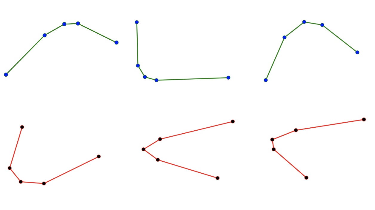
Figure 1: Microtubule buckle structures with 5 landmarks. Upper row: without vimentin filaments. Lower row: in the presence of vimentin filaments (generating stiffness).

Table 1: Reporting fraction of rejected hypothesis of equality of means using 100 simulations of two-sample test at nominal level $\alpha=0.05$ based on quantiles (top row) and a suitable bootstrap procedure (bottom row) under equality (left column) and under inequality (right column).

	Both with vimentin	One with and the other without vimentin
Quantile based	0.11	0.37
Bootstrap based	0.03	0.84

References

- Bhattacharya and Lin (2017) Bhattacharya, R. and L. Lin (2017). Omnibus CLTs for Fréchet means and nonparametric inference on non-Euclidean spaces. Proceedings of the American Mathematical Society 145(1), 413–428.
- Bhattacharya and Patrangenaru (2005) Bhattacharya, R. N. and V. Patrangenaru (2005). Large sample theory of intrinsic and extrinsic sample means on manifolds II. The Annals of Statistics 33(3), 1225–1259.
- Cheeger and Ebin (2008) Cheeger, J. and D. G. Ebin (2008). Comparison theorems in Riemannian geometry, Volume 365. American Mathematical Soc.
- Dryden and Mardia (2016) Dryden, I. L. and K. V. Mardia (2016). Statistical Shape Analysis (2nd ed.). Chichester: Wiley.
- Eltzner and Huckemann (2019) Eltzner, B. and S. F. Huckemann (2019). A smeary central limit theorem for manifolds with application to high-dimensional spheres. Ann. Statist. 47(6), 3360–3381.
- Eltzner et al. (2021) Eltzner, B., S. Hundrieser, and S. F. Huckemann (2021). Finite sample smeariness on spheres.
- Hendriks and Landsman (1998) Hendriks, H. and Z. Landsman (1998). Mean location and sample mean location on manifolds: asymptotics, tests, confidence regions. Journal of Multivariate Analysis 67, 227–243.
- Hotz and Huckemann (2015) Hotz, T. and S. Huckemann (2015). Intrinsic means on the circle: Uniqueness, locus and asymptotics. Annals of the Institute of Statistical Mathematics 67(1), 177–193.
- Huckemann (2011a) Huckemann, S. (2011a). Inference on 3D Procrustes means: Tree boles growth, rank-deficient diffusion tensors and perturbation models. Scandinavian Journal of Statistics 38(3), 424–446.
- Huckemann (2011b) Huckemann, S. (2011b). Intrinsic inference on the mean geodesic of planar shapes and tree discrimination by leaf growth. The Annals of Statistics 39(2), 1098–1124.
- Hundrieser et al. (2020) Hundrieser, S., B. Eltzner, and S. F. Huckemann (2020). Finite sample smeariness of Fréchet means and application to climate.
- Le and Barden (2014) Le, H. and D. Barden (2014). On the measure of the cut locus of a Fréchet mean. Bulletin of the London Mathematical Society 46(4), 698–708.
- Nash (1956) Nash, J. (1956). The imbedding problem for Riemannian manifolds. The Annals of Mathematics 63, 20–63.
- Nolting et al. (2014) Nolting, J.-F., W. Möbius, and S. Köster (2014). Mechanics of individual keratin bundles in living cells. Biophysical journal 107(11), 2693–2699.
- Tran (2019) Tran, D. (2019). Behavior of Fréchet mean and central limit theorems on spheres. Brasilian Journal of Probability and Statistics, arXiv preprint arXiv:1911.01985. to appear.
- Tran et al. (2021) Tran, D., B. Eltzner, and S. F. Huckemann (2021). Reflection and reverse labeling shape spaces and analysis of microtubules buckling. manuscript.