Emergent $\mathcal{PT}$-symmetry breaking of Anderson-Bogoliubov modes in Fermi superfluids

Abstract

The spontaneous breaking of parity-time ($\mathcal{PT}$) symmetry, which yields rich critical behavior in non-Hermitian systems, has stimulated much interest. Whereas most previous studies were performed within the single-particle or mean-field framework, exploring the interplay between $\mathcal{PT}$ symmetry and quantum fluctuations in a many-body setting is a burgeoning frontier. Here, by studying the collective excitations of a Fermi superfluid under an imaginary spin-orbit coupling, we uncover an emergent $\mathcal{PT}$-symmetry breaking in the Anderson-Bogoliubov (AB) modes, whose quasiparticle spectra undergo a transition from being completely real to completely imaginary, even though the superfluid ground state retains an unbroken $\mathcal{PT}$ symmetry. The critical point of the transition is marked by a non-analytic kink in the speed of sound, as the latter completely vanishes at the critical point where the system is immune to low-frequency perturbations. These critical phenomena derive from the presence of a spectral point gap in the complex quasiparticle dispersion, and are therefore topological in origin.

Introduction.– The eigenspectrum of a parity-time ($\mathcal{PT}$)-symmetric Hamiltonian is either completely real, or formed by complex conjugate pairs, depending on the symmetry of its eigenstates Bender and Boettcher (1998); El-Ganainy et al. (2018); Bender et al. (2018). By tuning system parameters, the $\mathcal{PT}$ symmetry of eigenstates can be spontaneously broken across critical (or exceptional) points Moiseyev (2011), where coalescing eigenstates and eigenenergies give rise to intriguing critical phenomena. $\mathcal{PT}$-symmetry breaking and the critical phenomena thereof have been extensively studied in the past decades, over a plethora of physical systems ranging from photonics Feng et al. (2017); Pile (2017); Limonov et al. (2017); Horiuchi (2017); Xiao et al. (2019); Klauck et al. (2019); Szameit et al. (2011); Regensburger et al. (2012); Zhen et al. (2015); Weimann et al. (2017); Kim et al. (2016); Cerjan et al. (2016); Poshakinskiy et al. (2016), acoustics and phononics Cummer et al. (2016), to single spins Wu et al. (2019); Liu et al. (2020), quantum gases Li et al. (2019a) and superconducting wires Rubinstein et al. (2007); Chtchelkatchev et al. (2012). Most of these prior studies relied on single-particle or mean-field descriptions. Moving forward, the interplay of $\mathcal{PT}$-symmetry breaking and many-body correlations, which lies at the cutting edge of the current research, is expected to yield rich and exotic critical behavior Ashida et al. (2017); Zhou and Yu (2019); Pan et al. (2020a).

In this work, we theoretically demonstrate an emergent $\mathcal{PT}$-symmetry breaking in the collective modes of a Fermi superfluid, and investigate in detail the rich many-body critical phenomena therein. Specifically, we study the pairing superfluid and collective excitations of a two-component Fermi gas under a non-Hermitian, $\mathcal{PT}$-symmetric spin-orbit coupling (SOC). Characterized by a non-Hermitian extension of the Bardeen-Cooper-Schrieffer (BCS) theory, the ground state of the system is a $\mathcal{PT}$-symmetry-preserving superfluid with real energy. Intriguingly though, the Bogoliubov quasiparticle excitations above the BCS state feature complex dispersions, forming closed spectral loops on the complex plane. The ground state can therefore be regarded as a point-gap topological superfluid, insofar as it possesses both the pairing order and a spectral winding topology  Gong et al. (2018); Kawabata et al. (2019); Bergholtz et al. (2019); Okuma et al. (2020); Zhang et al. (2020) regarding its quasiparticle excitations.

More important, the Anderson-Bogoliubov (AB) collective modes of the superfluid undergo a $\mathcal{PT}$-symmetry transition as the SOC strength is tuned, while the superfluid ground state remains $\mathcal{PT}$-symmetry unbroken. In particular, a critical SOC strength exists, separating $\mathcal{PT}$-symmetry unbroken and broken phases of the AB modes that have purely real or imaginary spectra, respectively. As a prominent feature of the emergent $\mathcal{PT}$ transition, the phonon mode softens near the critical point, as the speed of sound vanishes in a kink at the transition. Such a critical behavior originates from the complete disappearance of low-frequency components in the density response function, a phenomenon protected by the point-gap topology of the quasiparticle dispersion. This suggests a topologically robust, critical superfluid state immune to low-frequency perturbations. Our work provides a unique paradigm for exploring emergent $\mathcal{PT}$-symmetry breaking and critical phenomena, and sheds new light on the study of quantum criticality in open many-body systems.

Model.–We consider a two-component, attractively interacting Fermi gas in three dimensions. The Fermi gas is loaded in an optical lattice and subject to a one-dimensional, imaginary SOC, with the Hamiltonian

$$\begin{split}H=&-2\sum_{\boldsymbol{k}}C_{\boldsymbol{k}}^{\dagger}(\sum_{\zeta=x,y,z}t_{s,\zeta}\cos k_{\zeta}+it_{so}\sigma_{z}\sin k_{x})C_{\boldsymbol{k}}\\ &-\frac{U}{V}\sum_{\boldsymbol{k},\boldsymbol{k}^{{}^{\prime}},\boldsymbol{q}}c_{\boldsymbol{q}+\boldsymbol{k}\uparrow}^{\dagger}c_{\boldsymbol{q}-\boldsymbol{k}\downarrow}^{\dagger}c_{-\boldsymbol{q}-\boldsymbol{k}^{{}^{\prime}}\downarrow}c_{-\boldsymbol{q}+\boldsymbol{k}^{{}^{\prime}}\uparrow},\end{split}$$ (1)

where $C_{\boldsymbol{k}}=(\begin{array}[]{cc}c_{\boldsymbol{k}\uparrow}&c_{\boldsymbol{k}\downarrow}\end{array})^{T}$, with $c_{\boldsymbol{k}\sigma=\uparrow,\downarrow}^{\dagger}$ ($c_{\boldsymbol{k}\sigma}$) the creation (annihilation) operator of a spin-$\sigma$ fermion with quasimomentum $\boldsymbol{k}=(k_{x},k_{y},k_{z})$. $t_{s,\zeta}$ is the hopping rate in the $\zeta$ spatial direction, $t_{so}$ is the SOC strength, $\sigma_{z}$ is the Pauli matrix, and $U$ is the interaction strength with the quantization volume given by $V$. Here the imaginary SOC may be implemented using spin-dependent dissipation Li et al. (2019a), non-reciprocal hopping Gou et al. (2020), or dissipative Raman processes Zhou et al. (2020).

Hamiltonian (1) is invariant under the combined transformation of the parity operator $\mathcal{P}:c_{\boldsymbol{k}\sigma}\rightarrow c_{-\boldsymbol{k}\sigma}$, and the time-reversal operator $\mathcal{T}:c_{\boldsymbol{k}\sigma}\rightarrow[i\sigma_{y}]_{\sigma\sigma^{{}^{\prime}}}c_{-\boldsymbol{k}\sigma^{{}^{\prime}}}$ and $i\rightarrow-i$ (or equivalently, $i\mathcal{K}\sigma_{y}$ with the complex conjugation operator $\mathcal{K}$ and Pauli matrix $\sigma_{y}$ in the first quantization), but possesses neither $\mathcal{P}$ nor $\mathcal{T}$ symmetry separately. Notably, although the single-particle spectra of Hamiltonian (1) are typically complex, the eigenenergies come in conjugate pairs, such that a non-interacting Fermi sea features a real Fermi energy.

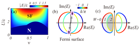
Figure 1: (a) Phase diagram on the $\nu$–$U$ plane, where the background colors indicate the order parameter $\Delta$. The self-consistent ground state of the system undergoes a first-order phase transition from the normal phase (N) to the superfluid phase (SF) when increasing $U$. (b)(c): Bogoliubov quasiparticle spectra in the limit $\Delta=0$ (the normal phase) (b) and SF phase (c) in the complex plane. As shown in (b), fermions in a potential Cooper pair are separated by a finite imaginary energy gap (vertical distance) on the Fermi surface, which underlies the first-order phase transition. The quasiparticle spectra are gapped in the SF phase [see (c)], which implies the emergence of quantized spectral winding number $W$ for the occupied bands (different shades of grey in (c) mark regions for different choice of reference energy). Here we take $t_{s}/\varepsilon=1$ and $t_{so}/\varepsilon=0.5$ with the unit of energy $\varepsilon=\hbar^{2}a^{-2}/(2m)$, where $a$ is the lattice constant (unit of length) and $m$ is the mass of fermions.

Non-Hermitian BCS formalism.– Pairing superfluidity has been investigated in open systems using non-Hermitian variations of the BCS formalism Kantian et al. (2009); Daley et al. (2009); Ghatak and Das (2018); Kawabata et al. (2018); Zhou and Cui (2019); Yamamoto et al. (2019). In the spirit of these studies, we define the $s$-wave pairing order parameters $\Delta=-(U/V)\sum_{\boldsymbol{k}}\langle c_{-\boldsymbol{k}\downarrow}c_{\boldsymbol{k}\uparrow}\rangle$ and $\bar{\Delta}=-(U/V)\sum_{\boldsymbol{k}}\langle c_{\boldsymbol{k}\uparrow}^{\dagger}c_{-\boldsymbol{k}\downarrow}^{\dagger}\rangle$. Note that $\bar{\Delta}\neq\Delta^{\ast}$ for general non-Hermitian systems Yamamoto et al. (2019); Ghatak and Das (2018). The non-Hermitian BCS mean-field Hamiltonian is given by

$$\hat{H}_{\text{BCS}}=\sum_{\boldsymbol{k}}C_{\boldsymbol{k}}^{\dagger}h_{\boldsymbol{k}}C_{\boldsymbol{k}}+\sum_{\boldsymbol{k}}(\Delta c_{\boldsymbol{k}\uparrow}^{\dagger}c_{-\boldsymbol{k}\downarrow}^{\dagger}+\bar{\Delta}c_{-\boldsymbol{k}\downarrow}c_{\boldsymbol{k}\uparrow}),$$ (2)

where a constant energy shift $V\Delta\bar{\Delta}/U$ is dropped. The BCS Hamiltonian can be diagonalized as $\hat{H}_{\text{BCS}}-\mu\hat{N}=\sum_{\boldsymbol{k}\sigma}E_{\boldsymbol{k}\sigma}\alpha_{\boldsymbol{k}\sigma}^{\dagger}\beta_{\boldsymbol{k}\sigma}$ (with the chemical potential $\mu$ and the total particle number operator $\hat{N}=\sum_{\boldsymbol{k}\sigma}c_{\boldsymbol{k}\sigma}^{\dagger}c_{\boldsymbol{k}\sigma}$) through the Bogoliubov transformations

$$\left(\begin{array}[]{c}\beta_{\boldsymbol{k}\uparrow}\\ \beta_{\boldsymbol{k}\downarrow}\end{array}\right)=U_{\boldsymbol{k}}\left(\begin{array}[]{c}c_{\boldsymbol{k}\uparrow}\\ c_{-\boldsymbol{k}\downarrow}^{\dagger}\end{array}\right),\left(\begin{array}[]{c}\alpha_{\boldsymbol{k}\uparrow}^{\dagger}\\ \alpha_{\boldsymbol{k}\downarrow}^{\dagger}\end{array}\right)=(U_{\boldsymbol{k}}^{-1})^{T}\left(\begin{array}[]{c}c_{\boldsymbol{k}\uparrow}^{\dagger}\\ c_{-\boldsymbol{k}\downarrow}\end{array}\right).$$ (3)

Here $U_{\boldsymbol{k}}=\left(\begin{array}[]{cc}u_{\boldsymbol{k}}&\upsilon_{\boldsymbol{k}}\\ -\bar{\upsilon}_{\boldsymbol{k}}&u_{\boldsymbol{k}}\end{array}\right)$, with $u_{\boldsymbol{k}}=\sqrt{\frac{1}{2}(1+\frac{\xi_{\boldsymbol{k}}}{E_{\boldsymbol{k}}})}$, $\upsilon_{\boldsymbol{k}}=\sqrt{\frac{\Delta}{2\bar{\Delta}}(1-\frac{\xi_{\boldsymbol{k}}}{E_{\boldsymbol{k}}})}$, $\bar{\upsilon}_{\boldsymbol{k}}=\sqrt{\frac{\bar{\Delta}}{2\Delta}(1-\frac{\xi_{\boldsymbol{k}}}{E_{\boldsymbol{k}}})}$, $\xi_{\boldsymbol{k}}=-2\sum_{\zeta=x,y,z}(t_{s,\zeta}\cos k_{\zeta}+it_{so}\sin k_{x})-\mu$, and $E_{\boldsymbol{k}}=\sqrt{\bar{\Delta}\Delta+\xi_{\boldsymbol{k}}^{2}}$. Under the convention $\sqrt{z}\geq 0$ for $z\in\mathbb{C}$, $E_{\boldsymbol{k}\sigma}=\pm E_{\boldsymbol{k}}$ are respectively identified as the quasiparticle (positive) and quasihole (negative) dispersions, with the corresponding field operators satisfying $\{\alpha_{\boldsymbol{k}\sigma}^{\dagger},\beta_{\boldsymbol{k}^{{}^{\prime}}\sigma^{{}^{\prime}}}\}=\delta_{\sigma\sigma^{{}^{\prime}}}\delta_{\boldsymbol{k}\boldsymbol{k}^{{}^{\prime}}}$ and $\{\alpha_{\boldsymbol{k}\sigma},\beta_{\boldsymbol{k}^{{}^{\prime}}\sigma^{{}^{\prime}}}\}=0$.

The ground BCS state of the system is then constructed by filling the quasihole band $E_{\boldsymbol{k}\downarrow}$, and is captured by the density matrix $\rho_{\text{BCS}}=|\Psi_{\text{BCS}}\rangle\langle\tilde{\Psi}_{\text{BCS}}|$, with $|\Psi_{\text{BCS}}\rangle\propto\prod_{\boldsymbol{k}}(u_{\boldsymbol{k}}-\upsilon_{\boldsymbol{k}}c_{\boldsymbol{k}\uparrow}^{\dagger}c_{-\boldsymbol{k}\downarrow}^{\dagger})|\text{vac}\rangle$ and $|\tilde{\Psi}_{\text{BCS}}\rangle\propto\prod_{\boldsymbol{k}}(u_{\boldsymbol{k}}^{\ast}-\bar{\upsilon}_{\boldsymbol{k}}^{\ast}c_{\boldsymbol{k}\uparrow}^{\dagger}c_{-\boldsymbol{k}\downarrow}^{\dagger})|\text{vac}\rangle$. Such a treatment is equivalent to the zero-temperature limit of the Gibbs-state assumption $\rho_{G}=\exp[-\beta(\hat{H}_{\text{BCS}}-\mu\hat{N})]$ in Ref. Yamamoto et al. (2019).

With the above understandings, the self-consistent gap (top row) and number (lower row) equations are

$$\left(\begin{array}[]{c}1\\ \nu\end{array}\right)=\frac{1}{2V}\sum_{\boldsymbol{k}}\left(\begin{array}[]{c}U/E_{\boldsymbol{k}}\\ 1-\xi_{\boldsymbol{k}}/E_{\boldsymbol{k}}\end{array}\right),$$ (4)

where the density $\nu=N_{a}/(2V)$, and the total particle number $N_{a}=\text{Tr}(\rho_{\text{BCS}}\hat{N})$. Using $\xi_{\boldsymbol{k}}=\xi^{\ast}_{-\boldsymbol{k}}$ under the $\mathcal{PT}$ symmetry, an inspection of the summation in Eq. (4) reveals that the product $\Delta\bar{\Delta}$ must be real for this equation to hold. Without loss of generality, we denote $\Delta=|\Delta|e^{i\theta}$ and $\bar{\Delta}=|\bar{\Delta}|e^{-i(\theta+n\pi)}$, where $\theta$ is an arbitrary phase and $n\in\mathbb{Z}$. Interestingly, under the $U(1)$ gauge transformation $c_{\boldsymbol{k}\sigma}\rightarrow e^{i\theta/2}c_{\boldsymbol{k}\sigma}$, $\Delta$ and $\bar{\Delta}$ both become real numbers, which leads to $\mathcal{PT}|\Psi_{\text{BCS}}\rangle=|\Psi_{\text{BCS}}\rangle$, $\mathcal{PT}|\tilde{\Psi}_{\text{BCS}}\rangle=|\tilde{\Psi}_{\text{BCS}}\rangle$, and $\mathcal{PT}\rho_{\text{BCS}}(\mathcal{PT})^{-1}=\rho_{\text{BCS}}$. The BCS ground state thus preserves the $\mathcal{PT}$ symmetry up to a U(1) gauge transformation, which suggests that the BCS ground-state energy is necessarily real.

Furthermore, we find that the BCS ground state always lies within the sector $\Delta\bar{\Delta}>0$. Considering the fact that the gap and number equations are only dependent on the product $\Delta$ and $\bar{\Delta}$, rather than their relative ratio, we take $\Delta^{\ast}=\bar{\Delta}$, which does not affect the physical conclusions of our work sup . For numerical calculations, we focus on a quasi-one-dimensional configuration, where the Fermi gas is tightly confined in the spatial directions perpendicular to that of the SOC, such that $t_{s,y,z}\ll t_{s,x}$. Integrating out the transverse degrees of freedom and replacing $V^{-1}\sum_{\boldsymbol{k}}$ with $L_{x}^{-1}\sum_{k_{x}}$ ($L_{x}$ being the lattice size long the $x$ direction) in Eq. (4), we self-consistently solve the gap and number equations for $\{\Delta,\mu\}$, from which the BCS ground state as well as Bogoliubov quasiparticle spectra are constructed. For convenience, we drop the label $x$ in the following discussions.

Point-gap topological superfluid.– In Fig. 1(a), we show the numerically calculated ground-state phase diagram. Unlike the conventional Hermitian case, where the superfluid phase transition is continuous, our model possesses a first-order phase boundary between the superfluid (SF) and the normal (N) phase, as evidenced by the plotted discontinuous color changes across the phase boundary. Such a behavior originates from the competition between the pairing interaction and an imaginary gap introduced by the non-Hermitian SOC [see Fig. 1(b)(c)]. Note that the phase transition becomes continuous in the vacuum limit with the particle density $\nu=N_{a}/L\rightarrow 0$.

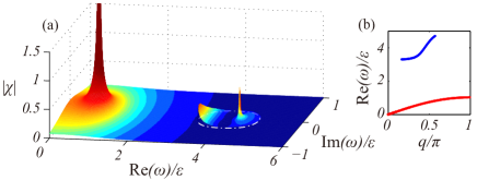
Figure 2: (a) Typical distribution of response function $\chi(q,\omega)$ on the complex frequency plane with a fixed $q/\pi=0.5$. The sharp peaks reflect the presence of collective modes. (b) Dispersions of collective modes, obtained from the sharp peaks plotted in panel (a). Note that the imaginary parts of the spectra are zero here, as we take $t_{so}<t_{s}$. The lower (higher) branch locates outside (inside) the loop $\omega=E_{k+q/2}+E_{k-q/2}$, which is marked by the dash-dotted curve in (a). Here we take the parameters $t_{s}/\varepsilon=1$, $t_{so}/\varepsilon=0.5$, $\nu=1/4$, $U/\varepsilon=4$.

In the superfluid phase, quasiparticle dispersions $E_{\boldsymbol{k}\sigma}$ form closed spectral loops on the complex plane, reminiscent of the eigenspectral point-gap topology associated with the seminal non-Hermitian skin effects Gong et al. (2018); Kawabata et al. (2019); Bergholtz et al. (2019); Okuma et al. (2020); Zhang et al. (2020); Pan et al. (2020b). The spectral winding number characterizing the ground-state point-gap topology is given by

$$W(\Omega)=\frac{1}{2\pi i}\int dk\frac{\partial}{\partial k}\arg[E_{k\downarrow}(k)-\Omega],$$ (5)

where $\Omega$ is the reference energy. In contrast to the normal phase, where the excitation spectra are gapless and $W$ is ill-defined, $W$ takes quantized values in the superfluid phase. As illustrated in Fig. 1(d), $W(\Omega)$ can take quantized values of $0$, $1$, or $2$, when $\Omega$ is chosen within different regimes. The absolute value of $W$ indicates the degeneracy of edge modes with eigenenergy $\Omega$, under a semi-infinite boundary condition  Okuma et al. (2020); Zhang et al. (2020); sup . This implies that the BCS state possesses not only pairing order parameter but also nontrivial point-gap topology, and thus represents a point-gap topological superfluid state sup . Whereas it is naturally expected that quasiparticle excitations of the superfluid would similarly be localized at the boundaries under an open boundary condition Yao and Wang (2018); Kunst et al. (2018); Lee (2016); Xiong (2018); Alvarez et al. (2018); McDonald et al. (2018); Lee and Thomale (2019); Li et al. (2019b); Yokomizo and Murakami (2019); Kawabata et al. (2019); Hofmann et al. (2020); Xiao et al. (2020); Helbig et al. (2020); Bergholtz et al. (2019), we instead focus here on the physics of collective modes, where the point-gap topological nature of the superfluid has a dramatic impact.

Spontaneous $\mathcal{PT}$-symmetry breaking of AB modes.– The spontaneous breaking of U(1) gauge symmetry by the pairing order generally leads to the emergence of gapless AB collective modes, which manifest themselves as the divergence in the linear response. We extend the conventional dynamic BCS theory Combescot et al. (2006) into the non-Hermitian regime, and derive the density response function

$$\chi(q,\omega)=\frac{1}{4\pi}(I^{{}^{\prime\prime}}-\left|\Delta\right|^{2}\frac{I^{2}I_{11}+\omega^{2}I^{{}^{\prime}2}I_{22}-2\omega^{2}I_{12}I^{{}^{\prime}}I}{I_{11}I_{22}-\omega^{2}I_{12}^{2}}),$$ (6)

where the response function $\chi(q,\omega)$ characterizes the density fluctuation of the superfluid to a small external perturbation of frequency $\omega$ and momentum $q$, and the definitions of integrals $\{I,I^{{}^{\prime}},I^{{}^{\prime\prime}},I_{11},I_{12},I_{22}\}$ are given in the Supplemental Material sup as functions of $\omega$ and $q$. To unravel the complete response feature of our model, we extend the definition of $\chi$ into the complex-frequency regime Xue et al. (2020); Li et al. (2021), which corresponds to the linear response of damped/amplified perturbations, when the frequency deviates from the real axis sup . Similar to the Hermitian case, the first term on the right hand side of Eq. (6) represents the linear-response results from the standard BCS theory, and the second term, being proportional to $|\Delta|^{2}$, represents contributions from quantum fluctuations of the pairing field that are responsible for the AB collective modes.

In general, $\chi$ has two types of poles: poles of $I^{{}^{\prime\prime}}$ which arise from the breaking of Cooper pairs into Bogoliubov quasiparticles (also applicable to poles of the integrals $\{I,I^{{}^{\prime}},I_{11},I_{12},I_{22}\}$); and poles of the second term in Eq. (6), which satisfy $I_{11}I_{22}=\omega^{2}I_{12}^{2}$, and originate from the AB collective modes Combescot et al. (2006). In a Hermitian BCS state, the first type of poles appear at the extremal frequencies of the function $\omega=E_{k+q/2}+E_{k-q/2}$, which correspond to irremovable singularities in the integrals. In our non-Hermitian system, however, since the frequency is extended to the complex regime, the spectral winding of quasiparticles guarantees that the extremal conditions of the real and complex components cannot occur simultaneously. The integrals therefore do not have singularities, and the first kind of poles completely disappear.

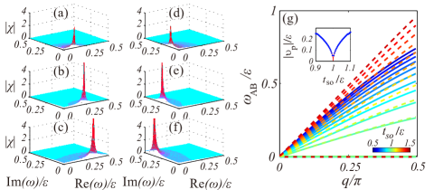
Figure 3: Response function $\chi(q,\omega)$ in the low-frequency regime for $t_{so}/\varepsilon=0.8$ ($t_{so}/\varepsilon=1.2$) in the left (right) column, with (a)(d) $q/\pi=0.1$; (b)(e) $q/\pi=0.2$; and (c)(f) $q/\pi=0.3$. (g) Spectra of AB modes $\omega_{AB}$ (solid: real part; dashed: imaginary part). The transition from solid to dashed lines as $t_{so}$ varies again illustrates the real-to-complex spectral transition shown in panels (a)-(f). Inset: numerically calculated speed of sound (blue dots) near the critical point, which is well-fitted by a power-law function $\propto|t_{s}-t_{so}|^{\gamma}$ (red curves), with a critical exponent $\gamma\approx 1/2$. Here we take $t_{s}/\varepsilon=1$, $U/\varepsilon=4$ and $\nu=1/4$.

In Fig. 2(a), we show the typical landscape of $\chi$ on the complex frequency plane. Two separate poles can be identified, one in the low-frequency regime, which is responsible for the low-frequency phonon mode; the other in the high-frequency regime. Both poles are characterized by $I_{11}I_{22}=\omega^{2}I_{12}^{2}$, and therefore contribute toward the AB collective modes. The high-frequency modes always lie within the spectral loop $\omega=E_{k+q/2}+E_{k-q/2}$, and are therefore gapped. In order to understand the gapless phonon excitations, we focus on the low-frequency regime [see the lower branch in Fig. 2(b)].

In Fig. 3, we show the response function in the low-frequency regime, with either small [(a)(b)(c)] or large [(d)(e)(f)] SOC strength. The location of sharp peaks satisfy $I_{11}I_{22}=\omega^{2}I_{12}^{2}$ (at the obvious pole of the response function), from which we solve for the dispersion of AB modes $\omega_{AB}(q)$ for different SOC strengths [see Fig. 3(g)]. Note that the resultant dispersions of AB modes change from purely real for $t_{so}<t_{s}$, to purely imaginary for $t_{so}>t_{s}$, thus indicating an intriguing transition point. This is in contrast to the BCS ground state that always features a real energy. Note that the spectra of the higher branch of the collective modes [see Fig. 2(b)] obtained from the sharp peaks plotted in Fig. 2(a)], are also real, regardless of the value of $t_{so}$. Thus, an emergent $\mathcal{PT}$-symmetry breaking occurs in the lower branch of the collective modes, at the critical point $t_{so}=t_{s}$. Close to the critical point, the speed of sound $\upsilon_{p}=\partial\omega_{AB}/\partial q\big{|}_{q=0}$, which characterizes the speed of propagation for phonon modes, rapidly vanishes toward a non-analytic kink at the transition point [see inset of Fig. 3(g)], confirming the existence of a quantum phase transition Sachdev (2007). The critical exponent, extracted from a numerical fit, is $\sim 1/2$.

Critical superfluid.– Here we focus on system’s behavior precisely at the critical point $t_{so}=t_{s}$. The real-to-complex transition at this point indicates that the low-frequency branch of the response function vanishes there, such that collective modes of the system are entirely determined by the high-frequency branch [see Fig. 4(a)]. We then have access to a peculiar scenario. As illustrated in the inset of Fig. 4(a), the total response function $\chi$ completely vanishes outside the spectral loop $\omega=E_{k+q/2}+E_{k-q/2}$ (the shaded region in the inset), even though contributions from the BCS theory (blue) and order-parameter fluctuations (black) remain finite. Physically, such a behavior suggests a critical superfluid that is immune to low-frequency perturbations. Remarkably, the total absence of linear response at the critical point can be analytically proven by changing the integrals in Eq. (6) into contour integrals on the complex plane, with the transformation $z=e^{ik}$. Given the spectral-loop structures of the Bogoliubov quasiparticles, all the integrals can be performed analytically through the Cauchy’s theorem sup . As such, the robustness of the critical superfluid is protected by the spectral point-gap topology of the Fermi quasiparticles.

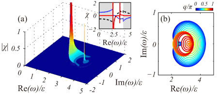
Figure 4: (a) Typical distribution of $|\chi|$ on the complex frequency plane at the critical point (take $q/\pi=0.5$ for example). Inset: the sectional view of $\chi$ along the real axis, where the red solid, blue dotted and black dashed curves denote the total, the part arising from the simple BCS theory, and the part arising from the order-parameter fluctuations of $\chi$, respectively. We can find $\chi$ vanishes exactly outside the gapped spectral loops of $\omega=E_{k+q/2}+E_{k-q/2}$ [see the shade regimes of the inset in (a)] for different $q$ (b). Here we set $U/\varepsilon=4$, $\delta t_{s}/\varepsilon=\delta t_{so}/\varepsilon=1$ and $\nu=1/4$.

Physically, the disappearance of linear response at the critical point can be understood through the exotic behavior of the BCS theory at the critical point. Explicitly, at the critical point, the quasiparticle spectrum is given by $E(z)=\sqrt{|\Delta|^{2}+(t_{s}z+\mu)^{2}}$, with $z=e^{ik}$ and $k\in[0,2\pi)$, which is analytic on the complex plane of $z$. The gap and number equations are therefore only determined by the residue near $z=0$, and can be reduced to

$$\frac{1}{U}=\frac{1}{2\sqrt{|\Delta|^{2}+\mu^{2}}},\quad\nu=\frac{1}{2}(1+\frac{\mu}{\sqrt{|\Delta|^{2}+\mu^{2}}}).$$ (7)

The above equations can be analytically solved, with the solutions $\mu=U(\nu-\frac{1}{2})$ and $|\Delta|=U\sqrt{\nu(1-\nu)}$. It is then straightforward to show that, at the critical point a first-order phase transition between the superfluid and normal phases occurs at $U=2t_{s}$, regardless of the density $\nu$. More importantly, since the BCS theory at the critical point is dispersionless, for a low-frequency perturbation, the impact on the system would be the same as that of a zero-momentum perturbation, which cannot lead to any fluctuations. The critical superfluid is only responsive to perturbations with a sufficiently high frequency, such that it lies within the spectral loop $\omega=E_{k+q/2}+E_{k-q/2}$ in the complex plane. Thus, we have shown that point-gap topology of quasiparticle excitations can be directly relevant when predicting many-body responses.

Final remarks.– We have uncovered an emergent $\mathcal{PT}$-symmetry breaking in the collective AB modes of a Fermi superfluid, and characterized in detail the exotic many-body critical phenomena at the transition point. In previous studies, $\mathcal{PT}$-symmetry breaking in the superconductivity fluctuations has been reported in superconducting wires Rubinstein et al. (2007); Chtchelkatchev et al. (2012). Their starting point, however, is the phenomenological Ginsburg-Landau field theory, and the dominant fluctuations therein originate from Cooper-pair breaking, rather than AB modes discussed here. Further, while we focus on a quasi-one-dimensional configuration, emergent $\mathcal{PT}$-symmetry breaking should also occur in higher dimensions, where the impact of dimensionality on the many-body critical phenomena would be an interesting open question for future studies.

Acknowledgements.–The authors wish to thank Dr. Sen Mu for very helpful discussions. J.-S. P. acknowledges the support from the National Natural Science Foundation of China (Grant No. 11904228) before he joined NUS. W. Y. acknowledges support by the National Natural Science Foundation of China (Grant No. 11974331), and the National Key R&D Program (Grant Nos. 2016YFA0301700, 2017YFA0304100). J. G. acknowledges funding support from Singapore National Research Foundation Grant No. NRF- NRFI2017-04 (WBS No. R-144-000-378-281).

Supplementary Material

In this Supplemental Material, we provide more details for the definition of point-gap topological superfluid state, self-consistent calculation of Bardeen-Cooper-Schrieffer (BCS) ground state, derivation of response function, and analytical calculation of linear response at the critical point of $\mathcal{PT}$-symmetry breaking.

.1 Point-gap topological superfluid

In this section, we provide more details for the definition and properties of point-gap topological superfluid state. Unlike the conventional Hermitian topological phase Hasan and Kane (2010); Qi and Zhang (2011); Chiu et al. (2016); Armitage et al. (2018); Nayak et al. (2008), the topological invariant of point-gap topology Gong et al. (2018); Kawabata et al. (2019); Bergholtz et al. (2019); Okuma et al. (2020); Zhang et al. (2020); Pan et al. (2020b) is defined upon the complex spectra, rather than the many-body ground-state wave functions. Such a spectral topology has been intensively discussed recently for single-particle energy bands in non-Hermitian systems with skin effects Yao and Wang (2018); Kunst et al. (2018); Lee (2016); Xiong (2018); Alvarez et al. (2018); McDonald et al. (2018); Lee and Thomale (2019); Hofmann et al. (2020); Xiao et al. (2020); Helbig et al. (2020); Bergholtz et al. (2019). By contrast, our point-gap topological invariant, i.e., the spectral winding number given in Eq. (6) in the main text, is defined for the occupied quasihole band $E_{k\downarrow}$, and thus reflects the spectral topological features of the BCS ground state.

While the spectral winding number $W$ is only meaningful for a specific reference energy $\Omega$, and thus inherently different from topological invariants of conventional topological matter, the resulting point-gap BCS state should acquire similar topological features associated with the spectral winding. For instance, under an open boundary condition, we expect all quasiparticle excitations above the BCS state to accumulate at the boundaries, driven by the non-Hermitian skin effects Yao and Wang (2018); Kunst et al. (2018); Lee (2016); Xiong (2018); Alvarez et al. (2018); McDonald et al. (2018); Lee and Thomale (2019); Li et al. (2019b); Yokomizo and Murakami (2019); Kawabata et al. (2019); Hofmann et al. (2020); Xiao et al. (2020); Helbig et al. (2020); Bergholtz et al. (2019). Further, under a semi-infinite configuration, where only one end of the quasi-one-dimensional system features a boundary, a continuum of edge modes would appear, whose degeneracy is dictated by the absolute value of the spectral winding number $W$ Gong et al. (2018); Kawabata et al. (2019); Bergholtz et al. (2019); Okuma et al. (2020); Zhang et al. (2020); Pan et al. (2020b). Although these aspects of the point-gap topological superfluid are intriguing and begs for further exploration, in the current work, we focus on the physics of collective modes, where the point-gap topology also plays a crucial role.

In Fig. S1, we show the phase diagram on the $\Delta$–$\mu$ plane (without solving self-consistent equations), where the color contour indicates the line gap $E_{h}$ [see Fig. S1(e)]. We find that, when $|\Delta|^{2}/t_{so}^{2}+\mu^{2}/t_{s}^{2}<1$, $E_{h}=0$, and $W$ is ill-defined. However, when $|\Delta|^{2}/t_{so}^{2}+\mu^{2}/t_{s}^{2}>1$, $E_{h}>0$ and $W$ is well-defined for any reference energy $\Omega$ that is not on the occupied spectral loop ($E_{k\downarrow}$). As shown in Fig. S1(e), $W$ has different quantized values in different regimes filled with different shades of gray. We also emphasize that, by solving the self-consistent equations, the gapless superfluid with $E_{h}=0$ and finite $|\Delta|$ is found to be unstable, such that the ground state of the system is either a gapped superfluid or a normal state.

.2 Self-consistent calculation of BCS ground state

In this section, we provide details on the self-consistent calculation of the BCS ground state. In the first column of Fig. S2, we show the self-consistent phase diagram for different spin-orbit coupling (SOC) strengths, where the red solid curves represent the first-order normal-superfluid phase boundaries. The superfluid states in the regimes enclosed by the red solid curves and dashed curves are metastable in the sense of that the energy is at a local minimum [see Fig. S2(d)(h)(i)]. Note that the metastable regime is not shown in the ground-state phase diagram in Fig. 1(a) of the main text. Interestingly, the normal-superfluid phase boundary becomes a straight line at critical point $t_{so}=t_{s}$, a phenomenon directly associated with the dispersionless, critical BCS theory (see discussions in the main text).

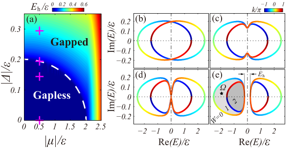
Figure S1: (a)Phase diagram on the plane of $\Delta$–$\mu$, without self-consistent calculations. The color contour represents $E_{h}$. (b)(c)(d)(e) Typical quasiparticle spectra corresponding to the crosses from bottom to top in (a), where the system is in the normal phase (b), the gapless superfluid phase (c), on the gapless-gapped phase boundary (d), and in the gapped superfluid phase (e). The boundary between the gapless and gapped superfluid phases (the dashed curve) is given by $|\Delta|^{2}/t_{so}^{2}+\mu^{2}/t_{s}^{2}=1$. As shown in (e), when the reference energy $\Omega$ is in different regimes specified with the shades, the spectral winding number $W$ takes different quantized values. Here we set $t_{s}/\varepsilon=1$ and $t_{so}/\varepsilon=0.1$.

.3 Response function

In this section, we provide details for the derivation of the response function using a non-Hermitian extension of the dynamic BCS theory Combescot et al. (2006); Combescot (1982). The response function characterizes the dynamics of superfluid state in the presence of small external perturbations. In the Hermitian limit, the dynamic BCS theory yields the same response function with that from the diagrammatical approach, but the former has a more straightforward physical picture Combescot et al. (2006).

Our starting point is the non-Hermitian BCS Hamiltonian

$$\hat{H}_{0}=\hat{H}_{\text{BCS}}-\mu\hat{N}=\sum_{k}(\begin{array}[]{cc}c_{k\uparrow}^{\dagger}&c_{-k\downarrow}\end{array})\left(\begin{array}[]{cc}\xi_{k}&\Delta\\ \bar{\Delta}&-\xi_{k}\end{array}\right)\left(\begin{array}[]{c}c_{k\uparrow}\\ c_{-k\downarrow}^{\dagger}\end{array}\right)=\sum_{k}(\begin{array}[]{cc}c_{k1}^{\dagger}&c_{k2}^{\dagger}\end{array})\hat{\epsilon}_{k}^{0,T}\left(\begin{array}[]{c}c_{k1}\\ c_{k2}\end{array}\right),$$ (S1)

where $c_{k1}=c_{k\uparrow}$, $c_{k2}=c_{-k\downarrow}^{\dagger}$, and $\hat{\epsilon}_{k}^{0}=\left(\begin{array}[]{cc}\xi_{k}&\bar{\Delta}\\ \Delta&-\xi_{k}\end{array}\right)$. To show that the response function is only dependent on $\bar{\Delta}\Delta$, as we claimed in the main text (which is not apparent here), we regard $\Delta^{\ast}$ and $\bar{\Delta}$ as different quantities throughout the derivation here. Assuming the density fluctuations are coupled with external perturbations of frequency $\omega$ and momentum $q$, the perturbation-fluctuation Hamiltonian is given by

$$\delta H=\sum_{k\lambda\lambda^{{}^{\prime}}}c_{k+q/2\lambda}^{\dagger}(\delta\hat{\epsilon}^{T})_{\lambda\lambda^{{}^{\prime}}}c_{k-q/2\lambda^{{}^{\prime}}}+h.c.,$$ (S2)

with $\delta\hat{\epsilon}=\left(\begin{array}[]{cc}\delta F&\delta\bar{\Delta}\\ \delta\Delta&-\delta F\end{array}\right)$, where $\delta F$ and $\delta\Delta$ respectively denote the external perturbations and the fluctuations of pairing field. Then the dynamic BCS Hamiltonian is given by

$$\hat{H}_{tot}=\hat{H}_{0}+\delta\hat{H},$$ (S3)

which also satisfies the parity symmetry $\mathcal{P}\hat{H}_{tot}\mathcal{P}^{-1}=\hat{H}_{tot}^{\dagger}$. The density response function is defined as

$$\chi\left(q,\omega\right)=\delta n/\delta F,\quad\delta n=L^{-1}\sum_{k}\left(\delta n_{k}\right)_{11},$$ (S4)

where $(\delta\hat{n}_{k})_{\lambda\lambda^{{}^{\prime}}=1,2}=\langle c_{k-q/2,\lambda}^{\dagger}c_{k+q/2,\lambda^{{}^{\prime}}}\rangle$.

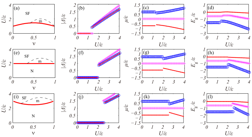
Figure S2: Self-consistent results of BCS theory when $t_{so}/t_{s}=0.5$ (top row), $1$ (middle row) and $1.5$ (bottom row): the phase diagram on the $\nu-U$ plane (a)(e)(h), superfluid order parameter $\Delta$ (b)(f)(i), chemical potential $\mu$ (c)(g) and ground-state energy $E_{g}$ (d)(h)(j). Different markers correspond to $\nu=0.25$ (red dots), $0.5$ (magenta crosses) and $0.75$ (blue circles), respectively. Here we fix $t_{s}/\varepsilon=1$.

Considering the time evolution of $|\Psi_{\text{BCS}}\rangle$ under $\hat{H}_{\text{tot}}$ in the Schrödinger picture, along with $\rho_{\text{BCS}}=|\Psi_{\text{BCS}}\rangle\langle\Psi_{\text{BCS}}|\mathcal{P}$ ($\mathcal{P}$ being the parity operator), we write down the Heisenberg equation $i\partial\langle\delta\hat{n}_{k}\rangle/\partial t=\langle\delta\hat{n}_{k}\hat{H}_{t}-\mathcal{P}^{-1}\hat{H}_{t}^{\dagger}\mathcal{P}\delta\hat{n}_{k}\rangle$, which can be simplified as

$$\omega\delta\hat{n}_{k}\approx\delta\hat{n}_{k}\hat{\epsilon}_{k+q/2}^{0}-\hat{\epsilon}_{k-q/2}^{0}\delta\hat{n}_{k}+\hat{n}_{k-q/2}^{0}\delta\hat{\epsilon}_{k}-\delta\hat{\epsilon}_{k}\hat{n}_{k+q/2}^{0}.$$ (S5)

Here we follow the spirit of linear response and write $\delta\hat{n}_{k}(t)\sim e^{i\omega t}\delta\hat{n}_{k}(0)$, where the matrix elements of the density operator $\hat{n}_{m}^{0}$ is given by $(\hat{n}_{k}^{0})_{\lambda\lambda^{{}^{\prime}}}=\langle c_{k\lambda}^{\dagger}c_{k\lambda{{}^{\prime}}}\rangle$. This is the kinetic equation that characterizes the fluctuation dynamics, formally the same as the Hermitian case Combescot et al. (2006), owing to the presence of an $\eta$-pseudo-Hermiticity $\hat{H}^{\dagger}_{\text{tot}}=\eta\hat{H}_{\text{tot}}\eta^{-1}$ with $\eta=\mathcal{P}$ in our model Mostafazadeh (2002a, b, c, d); Gardas et al. (2016). To unravel the complete response feature of our model, we discuss the response dynamics in the whole the complex-frequency regime Xue et al. (2020); Li et al. (2021), which corresponds to the linear response of damped/amplified perturbations when the frequency deviates from the real axis. The kinetic equation can be consistently solved with the dynamic extension of gap equation,

$$\sum_{k}\left[\left(\delta\hat{n}_{k}\right)_{12}+\frac{\delta\bar{\Delta}}{2E_{k}}\right]=0,\quad\sum_{k}\left[\left(\delta\hat{n}_{k}\right)_{21}+\frac{\delta\Delta}{2E_{k}}\right]=0,$$ (S6)

which are solved as follows.

Multiplied by $U_{k-q/2}$ and $U_{k+q/2}^{-1}$ respectively from the right and left sides, Eq. (S5) is cast into the form

$$\omega\delta\hat{\nu}_{k}=\delta\hat{\nu}_{k}\hat{E}_{k+q/2}^{0}-\hat{E}_{k-q/2}^{0}\delta\hat{\nu}_{k}+\hat{\nu}_{k-q/2}^{0}\delta\hat{E}_{k}-\delta\hat{E}_{k}\hat{\nu}_{k+q/2}^{0},$$ (S7)

where

$$\begin{split}&\delta\hat{\nu}_{k}=U_{k-q/2}\delta\hat{n}_{k}U_{k+q/2}^{-1},\quad\delta\hat{E}_{k}=U_{k-q/2}\delta\hat{\epsilon}_{k}U_{k+q/2}^{-1}\\ &\hat{E}_{k}^{0}=U_{k}\hat{\epsilon}_{k}^{0}U_{k}^{-1}=E_{k}\sigma_{z},\quad\hat{\nu}_{k}^{0}=U_{k}\hat{n}_{k}^{0}U_{k}^{-1}=\frac{1}{2}\left(1-\sigma_{z}\right).\end{split}$$ (S8)

It follows that

$$\delta\hat{\nu}_{k}=\left(\begin{array}[]{cc}0&\frac{-\left(\delta\hat{E}_{k}\right)_{12}}{\omega+\left(E_{+}+E_{-}\right)}\\ \frac{\left(\delta\hat{E}_{k}\right)_{21}}{\omega-\left(E_{+}+E_{-}\right)}&0\end{array}\right),$$ (S9)

and consequently

$$\left(\delta\hat{n}_{k}\right)_{11}=\frac{\left(\delta\hat{E}_{k}\right)_{12}}{\omega+\left(E_{+}+E_{-}\right)}u_{-}\bar{\upsilon}_{+}-\frac{\left(\delta\hat{E}_{k}\right)_{21}}{\omega-\left(E_{+}+E_{-}\right)}u_{+}\upsilon_{-},$$ (S10)

$$\left(\delta\hat{n}_{k}\right)_{12}=-\frac{\left(\delta\hat{E}_{k}\right)_{12}}{\omega+\left(E_{+}+E_{-}\right)}u_{+}u_{-}-\frac{\left(\delta\hat{E}_{k}\right)_{21}}{\omega-\left(E_{+}+E_{-}\right)}\upsilon_{+}\upsilon_{-},$$ (S11)

$$\left(\delta\hat{n}_{k}\right)_{21}=\frac{\left(\delta\hat{E}_{k}\right)_{21}}{\omega-\left(E_{+}+E_{-}\right)}u_{+}u_{-}+\frac{\left(\delta\hat{E}_{k}\right)_{12}}{\omega+\left(E_{+}+E_{-}\right)}\bar{\upsilon}_{+}\bar{\upsilon}_{-},$$ (S12)

where $E_{\pm}=E_{k\pm q}$, $u_{\pm}=u_{k\pm q}$, $\upsilon_{\pm}=\upsilon_{k\pm q}$ and $\bar{\upsilon}_{\pm}=\bar{\upsilon}_{k\pm q}$. From the definition of $\delta\hat{E}_{k}$ in Eq. (S8), we further have

$$\left(\delta\hat{n}_{k}\right)_{11}=\frac{1}{2}\frac{\delta F}{\omega^{2}-\left(E_{+}+E_{-}\right)^{2}}\left[\omega\left(\frac{\xi_{+}}{E_{+}}-\frac{\xi_{-}}{E_{-}}\right)+\left(E_{+}+E_{-}\right)\left(1+\frac{\bar{\Delta}\Delta-\xi_{+}\xi_{-}}{E_{+}E_{-}}\right)\right]$$

$$-\frac{1}{2}\frac{\delta\Delta}{\omega^{2}-\left(E_{+}+E_{-}\right)^{2}}\left[\omega+\left(E_{+}+E_{-}\right)\frac{\xi_{+}}{E_{+}}\right]\frac{\bar{\Delta}}{E_{-}}+\frac{1}{2}\frac{\delta\bar{\Delta}}{\omega^{2}-\left(E_{+}+E_{-}\right)^{2}}\left[\omega-\left(E_{+}+E_{-}\right)\frac{\xi_{-}}{E_{-}}\right]\frac{\Delta}{E_{+}},$$ (S13)

$$\left(\delta\hat{n}_{k}\right)_{12}=\frac{1}{2}\frac{\delta F}{\omega^{2}-\left(E_{+}+E_{-}\right)^{2}}\frac{\bar{\Delta}\left(E_{+}+E_{-}\right)\left[\omega-\left(\xi_{-}+\xi_{+}\right)\right]}{E_{+}E_{-}}$$

$$-\frac{1}{2}\frac{1}{\omega^{2}-\left(E_{+}+E_{-}\right)^{2}}\left\{\delta\bar{\Delta}\left[\omega\left(\frac{\xi_{+}}{E_{+}}+\frac{\xi_{-}}{E_{-}}\right)-\left(E_{+}+E_{-}\right)\left(1+\frac{\xi_{+}\xi_{-}}{E_{+}E_{-}}\right)\right]+\delta\Delta\left(E_{+}+E_{-}\right)\frac{\bar{\Delta}^{2}}{E_{+}E_{-}}\right\},$$ (S14)

$$\left(\delta\hat{n}_{k}\right)_{21}=-\frac{1}{2}\frac{\Delta\delta F\left(E_{+}+E_{-}\right)}{E_{+}E_{-}\left[\omega^{2}-\left(E_{+}+E_{-}\right)^{2}\right]}\left[\omega+\left(\xi_{+}+\xi_{-}\right)\right]$$

$$+\frac{1}{2}\frac{1}{\omega^{2}-\left(E_{+}+E_{-}\right)^{2}}\left\{\delta\Delta\left[\omega\left(\frac{\xi_{+}}{E_{+}}+\frac{\xi_{-}}{E_{-}}\right)+\left(E_{+}+E_{-}\right)\left(1+\frac{\xi_{+}\xi_{-}}{E_{+}E_{-}}\right)\right]-\delta\bar{\Delta}\left(E_{+}+E_{-}\right)\frac{\Delta^{2}}{E_{+}E_{-}}\right\}.$$ (S15)

We then solve for $\delta\Delta$ and $\delta\bar{\Delta}$ from Eqs. (S14) and (S15), with the help of Eq. (S6). As shown in Eqs. (S13), the density fluctuations $\left(\delta\hat{n}_{k}\right)_{11}$ and the response function can be derived after that. This process directly reflects the contribution of pairing-order dynamics in the density fluctuations.

Together with Eq. (S6), Eq. (S14) leads to

$$\begin{split}&-\delta\bar{\Delta}\sum_{k}\frac{1}{E_{k}}=\delta F\sum_{k}\frac{\bar{\Delta}}{\omega^{2}-\left(E_{+}+E_{-}\right)^{2}}\frac{\left(E_{+}+E_{-}\right)\left[\omega-\left(\xi_{-}+\xi_{+}\right)\right]}{E_{+}E_{-}}\\ &-\sum_{k}\frac{1}{\omega^{2}-\left(E_{+}+E_{-}\right)^{2}}\left\{\delta\bar{\Delta}\left[\omega\left(\frac{\xi_{+}}{E_{+}}+\frac{\xi_{-}}{E_{-}}\right)-\left(E_{+}+E_{-}\right)\left(1+\frac{\xi_{+}\xi_{-}}{E_{+}E_{-}}\right)\right]+\delta\Delta\left(E_{+}+E_{-}\right)\frac{\bar{\Delta}^{2}}{E_{+}E_{-}}\right\},\end{split}$$ (S16)

that is,

$$\begin{split}&-\bar{\Delta}\delta F\left[\omega I^{{}^{\prime}}\left(\omega,q\right)-I\left(\omega,q\right)\right]+\delta\bar{\Delta}\left\{\omega I_{12}\left(\omega,q\right)-\int dk\left[\frac{E_{+}E_{-}+\xi_{+}\xi_{-}}{\left(E_{+}+E_{-}\right)^{2}-\omega^{2}}-\frac{1}{E_{k}}\right]\right\}\\ &+\delta\Delta\int dk\frac{\bar{\Delta}^{2}}{\left(E_{+}+E_{-}\right)^{2}-\omega^{2}}=0.\end{split}$$ (S17)

For convenience, we list the various integral functions both in the above equations and in later ones

$$I_{12}=\int dk\frac{1}{E_{+}E_{-}}\frac{\xi_{+}E_{+}+\xi_{-}E_{-}}{(E_{+}+E_{-})^{2}-\omega^{2}},$$ (S18)

$$I_{11}=\int dk[\frac{(E_{+}+E_{-})}{E_{+}E_{-}}\frac{E_{+}E_{-}+\xi_{+}\xi_{-}+\bar{\Delta}\Delta}{(E_{+}+E_{-})^{2}-\omega^{2}}-\frac{1}{E}],$$ (S19)

$$\tilde{I}_{11}=\int dk[\frac{(E_{+}+E_{-})}{E_{+}E_{-}}\frac{E_{+}E_{-}+\xi_{+}\xi_{-}+\Delta^{2}}{(E_{+}+E_{-})^{2}-\omega^{2}}-\frac{1}{E}],$$ (S20)

$$\bar{\tilde{I}}_{11}=\int dk[\frac{(E_{+}+E_{-})}{E_{+}E_{-}}\frac{E_{+}E_{-}+\xi_{+}\xi_{-}+\bar{\Delta}^{2}}{(E_{+}+E_{-})^{2}-\omega^{2}}-\frac{1}{E}],$$ (S21)

$$I_{22}=\int dk[\frac{(E_{+}+E_{-})}{E_{+}E_{-}}\frac{E_{+}E_{-}+\xi_{+}\xi_{-}-\bar{\Delta}\Delta}{(E_{+}+E_{-})^{2}-\omega^{2}}-\frac{1}{E}],$$ (S22)

$$\tilde{I}_{22}=\int dk[\frac{(E_{+}+E_{-})}{E_{+}E_{-}}\frac{E_{+}E_{-}+\xi_{+}\xi_{-}-\Delta^{2}}{(E_{+}+E_{-})^{2}-\omega^{2}}-\frac{1}{E}],$$ (S23)

$$\bar{\tilde{I}}_{22}=\int dk[\frac{(E_{+}+E_{-})}{E_{+}E_{-}}\frac{E_{+}E_{-}+\xi_{+}\xi_{-}-\bar{\Delta}^{2}}{(E_{+}+E_{-})^{2}-\omega^{2}}-\frac{1}{E}],$$ (S24)

$$I=\int dk\frac{1}{E_{+}E_{-}}\frac{(\xi_{+}+\xi_{-})(E_{+}+E_{-})}{(E_{+}+E_{-})^{2}-\omega^{2}},$$ (S25)

$$I^{{}^{\prime}}=\int dk\frac{1}{E_{+}E_{-}}\frac{E_{+}+E_{-}}{(E_{+}+E_{-})^{2}-\omega^{2}},$$ (S26)

$$I^{{}^{\prime\prime}}=\int dk\frac{(E_{+}+E_{-})}{E_{+}E_{-}}\frac{E_{+}E_{-}-\xi_{+}\xi_{-}+\bar{\Delta}\Delta}{(E_{+}+E_{-})^{2}-\omega^{2}},$$ (S27)

$$\tilde{I}^{{}^{\prime\prime}}=\int dk\frac{(E_{+}+E_{-})}{E_{+}E_{-}}\frac{E_{+}E_{-}-\xi_{+}\xi_{-}+\Delta^{2}}{(E_{+}+E_{-})^{2}-\omega^{2}},$$ (S28)

$$\bar{\tilde{I}}^{{}^{\prime\prime}}=\int dk\frac{(E_{+}+E_{-})}{E_{+}E_{-}}\frac{E_{+}E_{-}-\xi_{+}\xi_{-}+\bar{\Delta}^{2}}{(E_{+}+E_{-})^{2}-\omega^{2}},$$ (S29)

where we have taken the approximation $2\pi L^{-1}\sum_{k}\rightarrow\int dk$ in the large-size limit.

Similarly, Eq. (S15) gives rise to

$$\begin{split}&-\Delta\delta F\left[-\omega I^{{}^{\prime}}\left(\omega,\boldsymbol{q}\right)-I\left(\omega,\boldsymbol{q}\right)\right]+\delta\Delta\left\{-\omega I_{12}\left(\omega,\boldsymbol{q}\right)-\int dk\left[\frac{E_{+}E_{-}+\xi_{+}\xi_{-}}{\left(E_{+}+E_{-}\right)^{2}-\omega^{2}}-\frac{1}{E_{k}}\right]\right\}\\ &+\delta\bar{\Delta}\int dk\frac{\Delta^{2}}{\left(E_{+}+E_{-}\right)^{2}-\omega^{2}}=0.\end{split}$$ (S30)

Then we have the following equalities

$$\begin{split}&\delta F\left[\omega\left(\Delta-\bar{\Delta}\right)I^{{}^{\prime}}+\left(\Delta+\bar{\Delta}\right)I\right]+\delta\bar{\Delta}\left(\omega I_{12}-\tilde{I}_{22}\right)+\delta\Delta\left(-\omega I_{12}-\bar{\tilde{I}}_{22}\right)=0,\\ &\delta F\left[-\omega\left(\Delta+\bar{\Delta}\right)I^{{}^{\prime}}-\left(\Delta-\bar{\Delta}\right)I\right]+\delta\bar{\Delta}\left(\omega I_{12}-\tilde{I}_{11}\right)-\delta\Delta\left(-\omega I_{12}-\bar{\tilde{I}}_{11}\right)=0,\end{split}$$ (S31)

which fix the relation between $\delta\Delta$, $\delta\bar{\Delta}$ and $\delta F$

$$\delta\Delta=-\frac{I\left[-\left(\Delta+\bar{\Delta}\right)\tilde{I}_{11}-\left(\Delta-\bar{\Delta}\right)\tilde{I}_{22}+2\Delta\omega I_{12}\right]+\omega I^{{}^{\prime}}\left[-\left(\Delta-\bar{\Delta}\right)\tilde{I}_{11}-\left(\Delta+\bar{\Delta}\right)\tilde{I}_{22}+2\Delta\omega I_{12}\right]}{\bar{\tilde{I}}_{22}\tilde{I}_{11}+\bar{\tilde{I}}_{11}\tilde{I}_{22}-2\omega^{2}I_{12}^{2}}\delta F,$$ (S32)

and

$$\delta\bar{\Delta}=-\frac{I\left[-\left(\Delta+\bar{\Delta}\right)\bar{\tilde{I}}_{11}+\left(\Delta-\bar{\Delta}\right)\bar{\tilde{I}}_{22}-2\omega\bar{\Delta}I_{12}\right]+\omega I^{{}^{\prime}}\left[-\left(\Delta-\bar{\Delta}\right)\bar{\tilde{I}}_{11}+\left(\Delta+\bar{\Delta}\right)\bar{\tilde{I}}_{22}+2\omega\bar{\Delta}I_{12}\right]}{\tilde{I}_{22}\bar{\tilde{I}}_{11}+\tilde{I}_{11}\bar{\tilde{I}}_{22}-2\omega I_{12}^{2}}\delta F.$$ (S33)

Substituting the forms of $\delta\Delta$ and $\delta\bar{\Delta}$ into the expression of $\left(\delta\hat{n}_{k}\right)_{11}$ in Eq. (S13), we finally have the expression for the linear response function

$$\chi(q,\omega)=\frac{L^{-1}\sum_{k}\left(\delta\hat{n}_{k}\right)_{11}}{\delta F}\approx\frac{1}{4\pi}\left[I^{{}^{\prime\prime}}-\bar{\Delta}\Delta\frac{I^{2}I_{11}+\omega^{2}I^{{}^{\prime}2}I_{22}-2\omega^{2}I_{12}I^{{}^{\prime}}I}{I_{11}I_{22}-\omega^{2}I_{12}^{2}}\right].$$ (S34)

The form of $\chi$ is indeed only dependent on the product of $\bar{\Delta}$ and $\Delta$, which justifies our practice of taking $\bar{\Delta}=\Delta^{\ast}$ in the main text.

.4 Analytical calculation of response function at the critical point

In this section, we present the analytical calculation of $\chi$ at the critical point of the $\mathcal{PT}$-symmetry breaking. When $\omega$ is outside the spectral loop $\omega=E_{+}+E_{-}$, the integrands of the integrals in Eq. (S18)-(S29) have only one singularity at $z=0$, with $z=e^{ik}$. Meanwhile, since $t_{so}=t_{s}$, these integrands are functions of $z$, rather than of both $z$ and $z^{\ast}$. The integrand are hence analytic everywhere on the complex plane, except for the singularity at $z=0$. According to the Cauchy’s integral theorem, we have the following analytical results

$$I_{12} =\oint_{|z|=1}dz\frac{1}{izE_{+}E_{-}}\frac{\xi_{+}E_{+}+\xi_{-}E_{-}}{(E_{+}+E_{-})^{2}-\omega^{2}}=2i\pi\lim_{z\rightarrow 0}\frac{z}{izE_{+}E_{-}}\frac{\xi_{+}E_{+}+\xi_{-}E_{-}}{(E_{+}+E_{-})^{2}-\omega^{2}}=2\pi\frac{-2\mu}{E_{0}}\frac{1}{4E_{0}^{2}-\omega^{2}},$$ (S35)

$$I_{11} =\oint_{|z|=1}dz\frac{1}{iz}[\frac{(E_{+}+E_{-})}{E_{+}E_{-}}\frac{E_{+}E_{-}+\xi_{+}\xi_{-}+\Delta^{2}}{(E_{+}+E_{-})^{2}-\omega^{2}}-\frac{1}{E}]=2\pi(\frac{2}{E_{0}}\frac{E_{0}^{2}+\mu^{2}+|\Delta|^{2}}{4E_{0}^{2}-\omega^{2}}-\frac{1}{E_{0}})=2\pi(\frac{4E_{0}}{4E_{0}^{2}-\omega^{2}}-\frac{1}{E_{0}}),$$ (S36)

$$I_{22} =\oint_{|z|=1}dz\frac{1}{iz}[\frac{(E_{+}+E_{-})}{E_{+}E_{-}}\frac{E_{+}E_{-}+\xi_{+}\xi_{-}-|\Delta|^{2}}{(E_{+}+E_{-})^{2}-\omega^{2}}-\frac{1}{E}]=2\pi(\frac{4\mu^{2}}{E_{0}}\frac{1}{4E_{0}^{2}-\omega^{2}}-\frac{1}{E_{0}}),$$ (S37)

$$I =\oint_{|z|=1}dz\frac{1}{iz}\frac{1}{E_{+}E_{-}}\frac{(\xi_{+}+\xi_{-})(E_{+}+E_{-})}{(E_{+}+E_{-})^{2}-\omega^{2}}=2\pi\frac{-4\mu}{E_{0}}\frac{1}{4E_{0}^{2}-\omega^{2}},$$ (S38)

$$I^{{}^{\prime}} =\oint_{|z|=1}dz\frac{1}{iz}\frac{1}{E_{+}E_{-}}\frac{E_{+}+E_{-}}{(E_{+}+E_{-})^{2}-\omega^{2}}=2\pi\frac{2}{E_{0}}\frac{1}{4E_{0}^{2}-\omega^{2}},$$ (S39)

$$I^{{}^{\prime\prime}} =\oint_{|z|=1}dz\frac{1}{iz}\frac{(E_{+}+E_{-})}{E_{+}E_{-}}\frac{E_{+}E_{-}-\xi_{+}\xi_{-}+|\Delta|^{2}}{(E_{+}+E_{-})^{2}-\omega^{2}}=2\pi\frac{4|\Delta|^{2}}{E_{0}}\frac{1}{4E_{0}^{2}-\omega^{2}}.$$ (S40)

Note that we have taken $\Delta^{\ast}=\bar{\Delta}$ in the above expressions. Further, we have

$$\frac{1}{(2\pi)^{3}}(4E_{0}^{2}-\omega^{2})^{2}(I^{2}I_{11}+\omega^{2}I^{{}^{\prime}2}I_{22}-2\omega^{2}I_{12}I^{{}^{\prime}}I)=\frac{-4\omega^{2}}{E_{0}^{3}},$$ (S41)

and

$$\frac{1}{(2\pi)^{2}}(4E_{0}^{2}-\omega^{2})^{2}(I_{11}I_{22}-\omega^{2}I_{12}^{2})=-\frac{\omega^{2}}{E_{0}^{2}}(4E_{0}^{2}-\omega^{2}),$$ (S42)

such that

$$\chi=\frac{1}{4\pi}\left[I^{{}^{\prime\prime}}-\left|\Delta\right|^{2}\frac{I^{2}I_{11}+\omega^{2}I^{{}^{\prime}2}I_{22}-2\omega^{2}I_{12}I^{{}^{\prime}}I}{I_{11}I_{22}-\omega^{2}I_{12}^{2}}\right]=\frac{2|\Delta|^{2}}{E_{0}}\frac{1}{4E_{0}^{2}-\omega^{2}}-\left|\Delta\right|^{2}\frac{\frac{-2\omega^{2}}{E_{0}^{3}}}{-\frac{\omega^{2}}{E_{0}^{2}}(4E_{0}^{2}-\omega^{2})}=0.$$ (S43)

This implies $\chi(q,\omega)$ completely vanishes outside the spectral loop $\omega=E_{+}+E_{-}$ at the critical point. The derivation indicates that the absence of response at the critical point is associated with the presence of a dispersionless (dynamic) BCS theory, as discussed in the main text.

References

Bender and Boettcher (1998)C. M. Bender and S. Boettcher, Physical Review Letters 80, 5243 (1998).
El-Ganainy et al. (2018)R. El-Ganainy, K. G. Makris, M. Khajavikhan,
Z. H. Musslimani,
S. Rotter, and D. N. Christodoulides, Nature Physics 14, 11 (2018).
Bender et al. (2018)C. M. Bender, R. Tateo,
P. E. Dorey, T. C. Dunning, G. Levai, S. Kuzhel, H. F. Jones, A. Fring, and D. W. Hook, PT symmetry: In quantum
and classical physics (World Scientific
Publishing, 2018).
Moiseyev (2011)N. Moiseyev, Non-Hermitian quantum
mechanics (Cambridge University Press, 2011).
Feng et al. (2017)L. Feng, R. El-Ganainy, and L. Ge, Nature Photonics 11, 752 (2017).
Pile (2017)F. P. D. Pile, Nature Photonics 11, 742 (2017).
Limonov et al. (2017)M. F. Limonov, M. V. Rybin,
A. N. Poddubny, and Y. S. Kivshar, Nature Photonics 11, 543 (2017).
Xiao et al. (2019)L. Xiao, K. Wang, X. Zhan, Z. Bian, K. Kawabata, M. Ueda, W. Yi, and P. Xue, Physical Review
Letters 123, 230401
(2019).
Klauck et al. (2019)F. Klauck, L. Teuber,
M. Ornigotti, M. Heinrich, S. Scheel, and A. Szameit, Nature Photonics 13, 883 (2019).
Szameit et al. (2011)A. Szameit, M. C. Rechtsman, O. Bahat-Treidel, and M. Segev, Physical Review A 84, 021806 (2011).
Regensburger et al. (2012)A. Regensburger, C. Bersch, M.-A. Miri,
G. Onishchukov, D. N. Christodoulides, and U. Peschel, Nature 488, 167 (2012).
Zhen et al. (2015)B. Zhen, C. W. Hsu,
Y. Igarashi, L. Lu, I. Kaminer, A. Pick, S.-L. Chua, J. D. Joannopoulos, and M. Soljačić, Nature 525, 354 (2015).
Weimann et al. (2017)S. Weimann, M. Kremer,
Y. Plotnik, Y. Lumer, S. Nolte, K. G. Makris, M. Segev, M. C. Rechtsman, and A. Szameit, Nature Materials 16, 433 (2017).
Kim et al. (2016)K.-H. Kim, M.-S. Hwang,
H.-R. Kim, J.-H. Choi, Y.-S. No, and H.-G. Park, Nature Communications 7, 1 (2016).
Cerjan et al. (2016)A. Cerjan, A. Raman, and S. Fan, Physical Review Letters 116, 203902 (2016).
Poshakinskiy et al. (2016)A. Poshakinskiy, A. Poddubny, and A. Fainstein, Physical Review Letters 117, 224302 (2016).
Cummer et al. (2016)S. A. Cummer, J. Christensen,
and A. Alù, Nature Reviews
Materials 1, 1 (2016).
Wu et al. (2019)Y. Wu, W. Liu, J. Geng, X. Song, X. Ye, C.-K. Duan, X. Rong, and J. Du, Science 364, 878 (2019).
Liu et al. (2020)W. Liu, Y. Wu, C.-K. Duan, X. Rong, and J. Du, arXiv preprint arXiv:2002.06798 (2020).
Li et al. (2019a)J. Li, A. K. Harter,
J. Liu, L. de Melo, Y. N. Joglekar, and L. Luo, Nature Communications 10, 1 (2019a).
Rubinstein et al. (2007)J. Rubinstein, P. Sternberg, and Q. Ma, Physical
Review Letters 99, 167003 (2007).
Chtchelkatchev et al. (2012)N. Chtchelkatchev, A. Golubov, T. Baturina, and V. Vinokur, Physical Review
Letters 109, 150405
(2012).
Ashida et al. (2017)Y. Ashida, S. Furukawa, and M. Ueda, Nature Communications 8, 1 (2017).
Zhou and Yu (2019)Z. Zhou and Z. Yu, Physical Review
A 99, 043412 (2019).
Pan et al. (2020a)L. Pan, X. Wang, X. Cui, and S. Chen, Physical Review A 102, 023306 (2020a).
Gong et al. (2018)Z. Gong, Y. Ashida,
K. Kawabata, K. Takasan, S. Higashikawa, and M. Ueda, Physical Review X 8, 031079 (2018).
Kawabata et al. (2019)K. Kawabata, K. Shiozaki,
M. Ueda, and M. Sato, Physical Review X 9, 041015 (2019).
Bergholtz et al. (2019)E. J. Bergholtz, J. C. Budich, and F. K. Kunst, arXiv
preprint arXiv:1912.10048 (2019).
Okuma et al. (2020)N. Okuma, K. Kawabata,
K. Shiozaki, and M. Sato, Physical Review Letters 124, 086801 (2020).
Zhang et al. (2020)K. Zhang, Z. Yang, and C. Fang, Physical Review Letters 125, 126402 (2020).
Gou et al. (2020)W. Gou, T. Chen, D. Xie, T. Xiao, T.-S. Deng, B. Gadway, W. Yi, and B. Yan, Physical Review Letters 124, 070402 (2020).
Zhou et al. (2020)L. Zhou, W. Yi, and X. Cui, Physical Review A 102, 043310 (2020).
Kantian et al. (2009)A. Kantian, M. Dalmonte,
S. Diehl, W. Hofstetter, P. Zoller, and A. Daley, Physical Review Letters 103, 240401 (2009).
Daley et al. (2009)A. Daley, J. Taylor,
S. Diehl, M. Baranov, and P. Zoller, Physical Review Letters 102, 040402 (2009).
Ghatak and Das (2018)A. Ghatak and T. Das, Physical Review
B 97, 014512 (2018).
Kawabata et al. (2018)K. Kawabata, Y. Ashida,
H. Katsura, and M. Ueda, Physical Review B 98, 085116 (2018).
Zhou and Cui (2019)L. Zhou and X. Cui, Iscience 14, 257 (2019).
Yamamoto et al. (2019)K. Yamamoto, M. Nakagawa,
K. Adachi, K. Takasan, M. Ueda, and N. Kawakami, Physical Review Letters 123, 123601 (2019).
(40) In this Supplemental Material, in which
the
Refs. Hasan and Kane (2010); Qi and Zhang (2011); Chiu et al. (2016); Armitage et al. (2018); Nayak et al. (2008); Gong et al. (2018); Kawabata et al. (2019); Bergholtz et al. (2019); Okuma et al. (2020); Zhang et al. (2020); Pan et al. (2020b); Yao and Wang (2018); Kunst et al. (2018); Lee (2016); Xiong (2018); Alvarez et al. (2018); McDonald et al. (2018); Lee and Thomale (2019); Li et al. (2019b); Yokomizo and Murakami (2019); Hofmann et al. (2020); Xiao et al. (2020); Helbig et al. (2020); Xue et al. (2020); Li et al. (2021); Combescot et al. (2006); Combescot (1982); Mostafazadeh (2002a, b, c, d); Gardas et al. (2016) are cited, we provide more details for
the definition of point-gap topological superfluid state, self-consistent
calculation of Bardeen-Cooper-Schrieffer (BCS) ground state, derivation of
response function, and analytical calculation of linear response at the
critical point of -symmetry breaking.
Pan et al. (2020b)J.-S. Pan, L. Li, and J. Gong, arXiv preprint arXiv:2010.14862 (2020b).
Yao and Wang (2018)S. Yao and Z. Wang, Physical Review
Letters 121, 086803
(2018).
Kunst et al. (2018)F. K. Kunst, E. Edvardsson,
J. C. Budich, and E. J. Bergholtz, Physical Review
Letters 121, 026808
(2018).
Lee (2016)T. E. Lee, Physical
Review Letters 116, 133903 (2016).
Xiong (2018)Y. Xiong, Journal
of Physics Communications 2, 035043 (2018).
Alvarez et al. (2018)V. M. Alvarez, J. B. Vargas,
M. Berdakin, and L. F. Torres, The European
Physical Journal Special Topics 227, 1295 (2018).
McDonald et al. (2018)A. McDonald, T. Pereg-Barnea, and A. A. Clerk, Physical Review X 8, 041031 (2018).
Lee and Thomale (2019)C. H. Lee and R. Thomale, Physical Review
B 99, 201103 (2019).
Li et al. (2019b)L. Li, C. H. Lee, and J. Gong, Physical Review B 100, 075403 (2019b).
Yokomizo and Murakami (2019)K. Yokomizo and S. Murakami, Physical Review Letters 123, 066404 (2019).
Hofmann et al. (2020)T. Hofmann, T. Helbig,
F. Schindler, N. Salgo, M. Brzezińska, M. Greiter, T. Kiessling, D. Wolf, A. Vollhardt, A. Kabaši, et al., Physical Review Research 2, 023265 (2020).
Xiao et al. (2020)L. Xiao, T. Deng, K. Wang, G. Zhu, Z. Wang, W. Yi, and P. Xue, Nature Physics 16, 761 (2020).
Helbig et al. (2020)T. Helbig, T. Hofmann,
S. Imhof, M. Abdelghany, T. Kiessling, L. W. Molenkamp, C. Lee, A. Szameit, M. Greiter, and R. Thomale, Nature Physics 16, 7 (2020).
Combescot et al. (2006)R. Combescot, M. Y. Kagan, and S. Stringari, Physical Review A 74, 042717 (2006).
Xue et al. (2020)W.-T. Xue, M.-R. Li,
Y.-M. Hu, F. Song, and Z. Wang, arXiv preprint arXiv:2004.09529 (2020).
Li et al. (2021)L. Li, S. Mu, C. H. Lee, and J. Gong, arXiv preprint arXiv:2012.08799
(2021).
Sachdev (2007)S. Sachdev, Handbook of Magnetism and Advanced Magnetic Materials (2007).
Hasan and Kane (2010)M. Z. Hasan and C. L. Kane, Reviews
of Modern Physics 82, 3045 (2010).
Qi and Zhang (2011)X.-L. Qi and S.-C. Zhang, Reviews of Modern
Physics 83, 1057
(2011).
Chiu et al. (2016)C.-K. Chiu, J. C. Teo,
A. P. Schnyder, and S. Ryu, Reviews of Modern Physics 88, 035005 (2016).
Armitage et al. (2018)N. Armitage, E. Mele, and A. Vishwanath, Reviews of Modern
Physics 90, 015001
(2018).
Nayak et al. (2008)C. Nayak, S. H. Simon,
A. Stern, M. Freedman, and S. D. Sarma, Reviews of Modern Physics 80, 1083 (2008).
Combescot (1982)R. Combescot, Journal of Low Temperature Physics 49, 295 (1982).
Mostafazadeh (2002a)A. Mostafazadeh, Journal of Mathematical Physics 43, 205 (2002a).
Mostafazadeh (2002b)A. Mostafazadeh, Journal of Mathematical Physics 43, 2814 (2002b).
Mostafazadeh (2002c)A. Mostafazadeh, Journal of Mathematical Physics 43, 3944 (2002c).
Mostafazadeh (2002d)A. Mostafazadeh, Nuclear Physics B 640, 419 (2002d).
Gardas et al. (2016)B. Gardas, S. Deffner, and A. Saxena, Scientific
Reports 6, 23408
(2016).