Fully Atomistic Modeling of Realistic Plasmonic Materials: Assessing the Performance of Iterative Solvers

Abstract

The fully atomistic modeling of real-size plasmonic nanostructures is computationally demanding, therefore most calculations are limited to small-to-medium sized systems. However, plasmonic properties strongly depend on the actual shape and size of the samples. In this paper we substantially extend the applicability of classical, fully atomistic approaches by exploiting state-of-the-art numerical iterative Krylov-based techniques. In particular, we focus on the recently developed $\omega$FQ model, when specified to carbon nanotubes, graphene-based nanostructures and metal nanoparticles. The performance of Generalized Minimal Residual (GMRES) and Quasi-Minimum Residual (QMR) algorithms is studied, with special emphasis on the dependence of the convergence rate on the dimension of the structures (up to 1 million atoms) and the physical parameters entering the definition of the atomistic approach.

I Introduction

Nanoplasmonics is an emerging field that has been significantly developed in the last decade.Liz-Marzán, Murphy, and Wang (2014); Stockman (2011) The optical properties of electron-free nanomaterials (e.g. metallic nanoparticles or graphene) are characterized by the rise of surface plasmons, which are coherent oscillations of the conduction electrons induced by an incoming radiation.Maier (2007) One of the peculiarities of such systems is that their plasmon resonance frequency (PRF) can be tuned as a function of the shape, size and supramolecular structure.Chen et al. (2008); Díez et al. (2009); Stewart et al. (2008); Lohse and Murphy (2013) In the particular case of graphene, PRF can also be tuned by exploiting electrical gating and chemical doping, which result in a modification of its Fermi energy, thus giving rise to many diverse applications, also in the technological field.Neto et al. (2009)

A peculiarity of plasmonic substrate is that their optical response strongly depends on the system’s size. In fact, small nanostructures do not experimentally exhibit the properties of larger structures.Cox, Silveiro, and García de Abajo (2016) Therefore, only the latter are actually exploited in real applications. These features strongly limit the role of modeling through full quantum mechanical (QM) descriptions, that are impracticable for real-size systems. For this reason, plasmonic structures are generally described by resorting to classical approachesJensen and Jensen (2008, 2009); Morton and Jensen (2010, 2011); Payton et al. (2012, 2014); Chen et al. (2015); Zakomirnyi et al. (2019); Li, Rinkevicius, and Ågren (2014); Zakomirnyi et al. (2020), and in particular through implicit models that describe the nanostructure as a continuum, and its optical properties in terms of the frequency-dependent complex permittivity.Draine (1988); Draine and Flatau (1994, 2013); Sutradhar, Paulino, and Gray (2008); Hohenester and Trügler (2012); Hohenester (2014); Corni and Tomasi (2001) Clearly, continuum methods lack any atomistic description of the substrates, which can instead be retained by using explicit, atomistic approaches, where the optical response directly arises from atomic parameters, as for instance computed frequency-dependent atomic complex polarizabilities.Jensen and Jensen (2008, 2009); Morton and Jensen (2010, 2011); Payton et al. (2012, 2014); Chen et al. (2015); Giovannini et al. (2019a, 2020) On the other hand, continuum approaches are not computationally demanding, because the Maxwell equations are solved on the surface of the nanostructure, while atomistic models require the treatment of all atoms, therefore the cost of the calculation scales as a function of the volume. This is the price to pay to describe for instance dopingN’Tsame Guilengui et al. (2012); Manjavacas, Nordlander, and García de Abajo (2012) and structural defectsAnand et al. (2014), which cannot be modelled by continuum approaches.

Due to the unfavourable scaling of classical atomistic models with the number of atoms, the calculation of the optical properties of real size structures, which are constituted by millions of atoms, is a hard task. Regardless of the specific discrete model, in fact, the calculation of the plasmonic response involves the solution of a number of complex-valued, frequency-dependent linear systems, with a dense coefficient matrix of order equal to the number of atoms. The solution of the linear system is challenging in terms of both memory requirements and computational cost, therefore the investigation of the performance and applicability of alternative numerical methods to approach this problem is particularly relevant and timely.

In this work we apply different numerical techniques to solve the problem. In particular, we model the optical response of large graphene-based structures by exploiting a fully atomistic, yet classical approach that has been recently developed by some of us, named $\omega$FQ.Giovannini et al. (2019a, 2020); Bonatti et al. (2020) There, each atom of the substrate is endowed with a charge, whose value is determined by solving a complex-valued linear system. The charge exchange between the atoms is governed by the Drude mechanism and by quantum tunneling. $\omega$FQ has recently been shown to be successfully applicable to both graphene-based materials and plasmonic metal nanoparticles, for which accurate results are obtained. However, similarly to all atomistic approaches, the solution of the $\omega$FQ linear system by means of direct methods based on the LU factorization of the system matrix scales unfavourably with the size of the nanostructure, therefore it is an ideal playground to test the performance of various solution algorithms based on Krylov subspace iterative methods,Van der Vorst (2003) such as the Generalized Minimal Residual (GMRES) and Quasi-Minimum Residual (QMR) algorithms.Saad and Schultz (1986); Freund and Nachtigal (1991) In particular, GMRES and QMR computational timing and convergence rates are compared with the direct inversion solution, which is also much more demanding in terms of memory requirements.

The manuscript is organized as follows. In the next section, we briefly recap the fundamentals of $\omega$FQ, by especially focusing on the mathematical properties of the $\omega$FQ linear system. Similarities and differences with continuum approaches are discussed, and Krylov-based methods are presented. We then apply the newly developed algorithms to the modeling of the plasmonic properties of selected nanostructures, of size up to hundreds of nanometer and constituted by roughly one million atoms. A summary and an overview of future developments end the manuscript.

II Theoretical Model

$\omega$FQ is a fully atomistic, classical model that describes the response of a system, such as nanoparticles or graphene-based nanostructures, to the external electric field $\mathbf{E}$.Giovannini et al. (2019a) In particular, each atom of the system is endowed with a charge. Charge exchange between different atoms is governed by the Drude mechanism of conduction,Jackson (2007) and modulated by quantum tunneling.Giovannini et al. (2019a) The key equation for solving the charges $\mathbf{q}$ reads:

$$\sum_{j=1}^{N}\bigg{(}\sum_{\begin{subarray}{c}k=1\\ k\neq i\end{subarray}}^{N}K_{ik}^{\mathrm{tot}}(D_{kj}-D_{ij})+\mathop{}\!\mathrm{i}\omega\bigg{)}q_{j}=\sum_{\begin{subarray}{c}j=1\\ j\neq i\end{subarray}}^{N}(V^{\mathrm{ext}}_{i}-V^{\mathrm{ext}}_{j})K^{\mathrm{tot}}_{ij},$$ (1)

where $V^{\mathrm{ext}}_{i}$ is the electric potential acting on the $i$-th charge associated with the external electric field oscillating at frequency $\omega$, $D_{ij}$ is the charge interaction kernel and $K^{\mathrm{tot}}_{ij}$ is a matrix accounting for both Drude and tunneling mechanisms.

More in detail, the linear system in eq. 1 describes the response of a set of $N$ complex-valued charges $q_{j}$ under the effect of an external monochromatic uniform electric field of frequency $\omega$ polarized along the $\hat{\mathbf{k}}$ direction, with $\hat{\mathbf{k}}=\hat{\mathbf{x}},\hat{\mathbf{y}},\hat{\mathbf{z}}$. The associated potential $V^{\mathrm{ext}}$ on each atom, entering the right-hand side of eq. 1, is defined as:

$$V^{\mathrm{ext}}_{i}=V^{\mathrm{ext}}(\mathbf{r}_{i})=-E^{k}_{0}k_{i},\qquad i=1,\dots,N,$$ (2)

where $E^{k}_{0}$ is the intensity of the electric field along the $k$ direction, $\mathbf{r}_{i}$ is the position of the $i$-th charge and $k_{i}$ is the component of $\mathbf{r}_{i}$ along the $\hat{\mathbf{k}}$ axis, i.e. $k_{i}=\mathbf{r}_{i}\cdot\hat{\mathbf{k}}$. The matrix $\mathbf{D}$ on the left-hand side of eq. 1 describes the electrostatic interaction between the charges, and it is defined in the standard formulation of the FQ force field exploited for treating molecular systems.Giovannini, Egidi, and Cappelli (2020a, b) In order to avoid the so-called “polarization catastrophe”, Jensen and Jensen (2008) instead of point charge we use spherical Gaussian charge distributions of width $d_{i}$ and $d_{j}$ to describe $\omega$FQ charges. $\mathbf{D}$ elements then read:Lipparini and Barone (2011); Giovannini et al. (2019a, b); Mayer (2007)

$$D_{ij}=\begin{cases}\frac{1}{r_{ij}}\mathrm{erf}\bigg{(}\frac{r_{ij}}{\sqrt{d_{i}^{2}+d_{j}^{2}}}\bigg{)}&i\neq j\\ \eta_{i}&i=j\end{cases},\quad i,j=1,\dots,N,$$ (3)

where $r_{ij}=\left|{\mathbf{r}_{i}-\mathbf{r}_{j}}\right|$ is the distance between charges $i$-th and $j$-th, $\mathrm{erf}$ is the error function and $\eta_{i}$ is the atomic chemical hardness of the $i$-th atom.Lipparini and Barone (2011); Rick, Stuart, and Berne (1994) Gaussian widths $d_{i}$ and $d_{j}$ are chosen for each atom by imposing that the limit for $\mathbf{r}_{i}\rightarrow\mathbf{r}_{j}$ corresponds to the diagonal element of the matrix, i.e.:

$$\lim_{\mathbf{r}_{i}\rightarrow\mathbf{r}_{j}}\frac{1}{r_{ij}}\mathrm{erf}\Bigg{(}\frac{r_{ij}}{\sqrt{d_{i}^{2}+d_{j}^{2}}}\Bigg{)}=\eta_{j}\quad\Rightarrow\quad d_{i}=\sqrt{\frac{2}{\pi}}\frac{1}{\eta_{j}}.$$ (4)

The D matrix can be formally seen as an overlap matrix defined in the scalar product weighted by the $\frac{1}{r}$ function. Therefore, it is symmetric positive definite (SPD).Lipparini and Barone (2011) The $\mathbf{K}^{\mathrm{tot}}$ matrix in eq. 1 reads:

$$\begin{split}K^{\mathrm{tot}}_{ij}=&(1-f(r_{ij}))K^{\mathrm{dru}}_{ij}(\omega)\\ =&(1-f(r_{ij}))\frac{2n_{0}}{1/\tau-\mathop{}\!\mathrm{i}\omega}\frac{\mathcal{A}_{ij}}{r_{ij}},\quad i,j=1,\dots,N,\ \ i\neq j,\end{split}$$ (5)

where $n_{0}$ is the electron density, $\tau$ is a friction-like constant due to scattering events and $\mathcal{A}_{ij}$ is an effective area dividing atoms $i$ and $j$. $f$ is a Fermi-like damping function, defined as:

$$f(r_{ij})=\frac{1}{1+\exp\bigg{[}-d\bigg{(}\frac{r_{ij}}{s\cdot r_{ij}^{0}}-1\bigg{)}\bigg{]}},$$ (6)

in which $r_{ij}^{0}$ is the equilibrium distance between atoms $i$ and $j$, while $d$ and $s$ are parameters ruling the shape of the damping function. $\mathbf{K}^{\mathrm{tot}}$ is a frequency-dependent symmetric complex-valued matrix, and it can be interpreted as a “dynamic” response matrix, whereas the D matrix describes the “static” response. It is worth noticing the expression of $\mathbf{K}^{\mathrm{tot}}$ can be associated with two alternative response regimes. When $f(r_{ij})$ goes to zero, the purely Drude conductive regime is recovered; as $r_{ij}$ increases, the electron transfer descreases exponentially, thus leading to the typical tunnelling mechanism.Giovannini et al. (2019a) The diagonal elements of $\mathbf{K}^{\mathrm{tot}}$ do not enter eq. 1, but the notation can be simplified by imposing $K^{\mathrm{tot}}_{ii}=0$ for all $i=1,\dots,N$ and extending the summations over $k$ and $j$ in eq. 1 to all $N$ atoms of the system.

As a final remark, the electron density $n_{0}$, that appears in eq. 5, is a specific property of the chemical composition of the plasmonic substrate and of the shape of the system. In a general 3D system, $n_{0}$ can be expressed as $n_{0}=\frac{\sigma_{0}/\tau}{m^{\star}}$, where $\sigma_{0}$ is the static conductance of the material, while $m^{\star}$ is its effective electron mass, which can be approximated to 1 for metal nanoparticles. However, in case of graphene-based materials, such as graphene sheets or carbon nanotubes, the effective electron mass needs to be taken into account.Giovannini et al. (2020) In graphene-based materials, $m^{\star}$ can be expressed as

$$m^{\star}=\frac{\sqrt{\pi n_{\mathrm{2D}}}}{v_{F}},$$ (7)

where $n_{\mathrm{2D}}$ is the 2D electron density of the system and $v_{F}$ is the Fermi velocity.Neto et al. (2009) The latter is related to the Fermi energy $\varepsilon_{F}$ through the expression $v_{F}=\sqrt{\frac{2\varepsilon_{F}}{m_{0}}}$, where $m_{0}$ is the electron rest mass.Neto et al. (2009) The 2D electron density $n_{\mathrm{2D}}$ can be calculated from $n_{0}$ as $n_{\mathrm{2D}}=n_{0}\cdot a_{0}$, with $a_{0}$ being the Bohr radius.Giovannini et al. (2020) Then, the 2D electron density can be calculated as the ratio of the number of atoms $N$ and the surface of the system $S$, i.e.:

$$n_{\mathrm{2D}}=\frac{\alpha N}{S},$$ (8)

where $\alpha$ is a parameter ($<1$) which selects the fraction of $\pi$ electrons which are involved in the studied plasmonic excitation.Giovannini et al. (2020) We note that such a parameter is uniquely determined by the value of $\varepsilon_{F}$.Giovannini et al. (2020)

II.1 Properties of the $\omega$FQ linear system

In this section, we analyze the mathematical properties of the $\omega$FQ linear system defined in eq. 1. We first notice that in eq. 5 the complex frequency-dependent ratio describing the Drude model can be gathered:

$$\begin{split}K^{\mathrm{tot}}_{ij}&=w(\omega)\overline{K}^{\mathrm{tot}}_{ij}=w(\omega)(1-f(r_{ij}))\frac{\mathcal{A}_{ij}}{r_{ij}},\\ w(\omega)&=\frac{2n_{0}}{1/\tau-\mathop{}\!\mathrm{i}\omega},\end{split}$$ (9)

where $\overline{\mathbf{K}}^{\mathrm{tot}}$ is a symmetric real-valued matrix. The frequency-dependent complex factor $w(\omega)$ is always non-zero, so we can take it out from eq. 1:

$$\sum_{j=1}^{N}\bigg{(}\sum_{k=1}^{N}\overline{K}_{ik}^{\mathrm{tot}}(D_{kj}-D_{ij})+\mathop{}\!\mathrm{i}\frac{\omega}{w(\omega)}\bigg{)}q_{j}=\sum_{j=1}^{N}(V^{\mathrm{ext}}_{i}-V^{\mathrm{ext}}_{j})\overline{K}^{\mathrm{tot}}_{ij}.$$ (10)

At this point we can introduce the following notation:

$$A_{ij} =\sum_{k=1}^{N}\overline{K}_{ik}^{\mathrm{tot}}(D_{kj}-D_{ij})$$ (11)

$$z(\omega) =-\mathop{}\!\mathrm{i}\frac{\omega}{w(\omega)}=-\frac{\omega}{2n_{0}\tau}(\omega\tau+\mathop{}\!\mathrm{i})$$ (12)

$$R_{i} =\sum_{j=1}^{N}(V^{\mathrm{ext}}_{i}-V^{\mathrm{ext}}_{j})\overline{K}^{\mathrm{tot}}_{ij},$$ (13)

and eq. 10 can be expressed in vector notation as

$$(\mathbf{A}-z(\omega)\mathbf{I})\mathbf{q}=\mathbf{R},$$ (14)

where $\mathbf{I}$ is the $N$-dimensional identity matrix. It can be noted that eq. 14 is fully equivalent to eq. 1, but $\mathbf{A}$ this time is a real-valued frequency-independent nonsymmetric matrix, of which the diagonal elements are shifted by a complex quantity. Moreover, the $\mathbf{A}$ matrix defined in eq. 11 can be rewritten as:

$$\begin{split}A_{ij}&=\sum_{k=1}^{N}\overline{K}^{\mathrm{tot}}_{ik}(D_{kj}-D_{ij})\\ &=\big{(}\overline{\mathbf{K}}^{\mathrm{tot}}\mathbf{D}\big{)}_{ij}-\bigg{(}\sum_{k=1}^{N}\overline{K}^{\mathrm{tot}}_{ik}\bigg{)}D_{ij}.\end{split}$$ (15)

By introducing a diagonal matrix $P_{il}=\big{(}\sum_{k=1}^{N}\overline{K}^{\mathrm{tot}}_{ik}\big{)}\delta_{il}$ where $\delta_{il}$ is the Kronecker delta, we can write:

$$\bigg{(}\sum_{k=1}^{N}\overline{K}^{\mathrm{tot}}_{ik}\bigg{)}D_{ij}=\sum_{l=1}^{N}P_{il}D_{lj},$$ (16)

and plugging the definition into eq. 15 we obtain:

$$\mathbf{A}=(\overline{\mathbf{K}}^{\mathrm{tot}}-\mathbf{P})\mathbf{D}.$$ (17)

Therefore, the $\mathbf{A}$ matrix can be formulated as the product of two real-valued symmetric matrices, since $\overline{\mathbf{K}}^{\mathrm{tot}}$ and $\mathbf{D}$ are symmetric and $\mathbf{P}$ is diagonal. However, $\mathbf{A}$ is a nonsymmetric matrix because $\mathbf{D}$ and $\overline{\mathbf{K}}^{\mathrm{tot}}-\mathbf{P}$ in general do not commute. Nevertheless, the following equality holds:

$$\mathbf{DA}=\mathbf{D}(\overline{\mathbf{K}}^{\mathrm{tot}}-\mathbf{P})\mathbf{D}=\big{[}(\overline{\mathbf{K}}^{\mathrm{tot}}-\mathbf{P})\mathbf{D}\big{]}^{T}\mathbf{D}=\mathbf{A}^{T}\mathbf{D},$$ (18)

where ^T indicates the transposition operator. Recalling that $\mathbf{D}$ is an SPD matrix,Lipparini and Barone (2011) we can define the $\mathbf{D}$-inner product as:

$$\forall\ \mathbf{x},\mathbf{y}\in\mathds{C}^{N}\quad\braket{\mathbf{x},\mathbf{y}}_{\mathbf{D}}=\braket{\mathbf{Dx},\mathbf{y}},$$ (19)

where $\braket{\cdot,\cdot}$ is the standard Euclidean inner product. From eq. 18 and eq. 19 it can be demostrated that $\mathbf{A}$ is self-adjoint with respect to the $\mathbf{D}$-inner product, i.e.:

$$\braket{\mathbf{Ax},\mathbf{y}}_{\mathbf{D}}=\braket{\mathbf{DAx},\mathbf{y}}=\braket{\mathbf{A}^{T}\mathbf{Dx},\mathbf{y}}=\braket{\mathbf{Dx},\mathbf{Ay}}=\braket{\mathbf{x},\mathbf{Ay}}_{\mathbf{D}}.$$ (20)

Equation 20 allows us to conclude that even if $\mathbf{A}$ is a nonsymmetric matrix, it is self-adjoint with respect to the inner product induced by the SPD matrix $\mathbf{D}$, therefore $\mathbf{A}$ is diagonalizable with real eigenvalues.

As a final remark, the alternative expression of the $\mathbf{A}$ matrix in eq. 17 allows us to derive another property of the matrix itself. In fact, $\overline{\mathbf{K}}^{\mathrm{tot}}-\mathbf{P}$ is such that each row (or column) sums up to zero, therefore it is a singular matrix. By this, the matrix $\mathbf{A}$ is also singular. Nevertheless, the existence and uniqueness of the linear system solution in eq. 14 is guaranteed through the diagonal shift of the coefficient matrix with the complex scalar $z(\omega)$ defined in eq. 12, which is non-zero when $\omega\neq 0$. However, numerical instabilities in the solution of the linear system can arise when $\omega$ approaches zero because $\mathbf{A}$ is close to singular.

II.2 Comparison with continuum approaches

The atomistic nature of $\omega$FQ emerges from all the variables that enter eq. 1: charge positions, chemical hardnesses in eq. 3, effective areas in eq. 5 and equilibrium distances in eq. 6, as well as electronic features of the material that enter the Drude model. Such an approach allows us to describe the (macroscopic) plasmonic response of the system in terms of (microscopic) atomistic quantities, regardless of the shape of the system. Therefore, complex effects associated with surface roughness and edge effects are automatically considered.

As stated in the Introduction, the plasmonic response of complex systems can be described by resorting to continuum approaches, such as the Boundary Element Method (BEM).De Abajo and Howie (2002); Hohenester and Trügler (2012) There, the material is treated as a continuum and its electronic properties are synthesized by its frequency-dependent dielectric permittivity function $\varepsilon(\omega)$. The plasmonic response arises as a surface charge density $\sigma(\mathbf{r})$, which is computed by solving Maxwell equations, via a reformulation as a boundary integral equation on the material surface. From the computational point of view, the latter is discretized in $N$ surface elements centered at positions $\mathbf{r}_{i}$, with $i=1,\dots,N$. At the same time, the surface charge density $\sigma(\mathbf{r})$ is discretized in terms of $N$ electric charges. The equation for solving the charges in BEM reads:Hohenester and Trügler (2012):

$$\bigg{(}2\pi\frac{\varepsilon_{\mathrm{out}}(\omega)+\varepsilon_{\mathrm{in}}(\omega)}{\varepsilon_{\mathrm{out}}(\omega)-\varepsilon_{\mathrm{in}}(\omega)}\mathbf{I}+\mathbf{F}\bigg{)}\bm{\sigma}=-\overline{\bm{\phi}},$$ (21)

where $\varepsilon_{\mathrm{out}},\varepsilon_{\mathrm{in}}$ are the frequency-dependent complex-valued dielectric permittivity functions of the outer (usually vacuo) and inner (the material) region, respectively, $\sigma_{i}=\sigma(\mathbf{r}_{i})$ is the electric charge evaluated on the surface element at position $\mathbf{r}_{i}$, while $\overline{\phi}_{i}=\frac{\partial\phi(\mathbf{r}_{i})}{\partial n}$ is the surface derivative of the external potential $\phi$ at position $\mathbf{r}_{i}$. Moreover, $\mathbf{I}$ is the $N$-dimensional identity matrix and $F_{ij}$ is the normal derivative of the Green function, i.e.:

$$F_{ij}=F(\mathbf{r}_{i},\mathbf{r}_{j})=\hat{\mathbf{n}}_{i}\cdot\nabla_{\mathbf{r}_{j}}\frac{1}{\left|{\mathbf{r}_{i}-\mathbf{r}_{j}}\right|},$$ (22)

where $\hat{\mathbf{n}}_{i}$ is the normal vector to the surface at point $\mathbf{r}_{i}$.

$\omega$FQ and BEM are genuinely different in terms of performance and versatility: surface roughness can easily be taken into account through an atomistic approach, while the continuum model needs specific treatments such as perturbative expansions.Trügler et al. (2011) Nevertheless, from the purely algebraic point of view, there are some similarities. First of all, eqs. 14 and 21 have the same structure. In both cases, charges are obtained by solving a dense system of linear equations, in which the left-hand side is written in terms of a nonsymmetric frequency-independent real-valued matrix [$\mathbf{A}$ for $\omega$FQ (see eq. 11 and $\mathbf{F}$ for BEM (see eq. 22)] with a uniform complex-valued diagonal shift, which describes the electronic properties of the material at a specific frequency ($z(\omega)$ defined in eq. 12 for $\omega$FQ and the permittivity in eq. 21 for BEM). Moreover, it has been shown that the $\mathbf{F}$ matrix in eq. 22 is singular and diagonalizable with real eigenvaluesHohenester and Trügler (2012); Fuchs (1975); Mayergoyz, Fredkin, and Zhang (2005); Fredkin and Mayergoyz (2003), similarly to the $\mathbf{A}$ matrix in eq. 11 (see section II.1 for the proof). Therefore, the same computational techniques to solve the linear system, which in this paper are described for the $\omega$FQ approach, can also be exploited for BEM.

III Solution strategies

In order to model the optical spectra of plasmonic substrates, eq. 1, or equivalently eq. 14, need to be solved for a certain number of frequencies $\omega$. This can effectively achieved only by resorting to efficient methods to solve the dense nonsymmetric complex linear system. This point is crucial, especially when the dimensionality of the system increases. Direct techniques of solution (e.g. based on factorization of the coefficient matrix) are to be avoided, because they are inefficient both in terms of storage demand and computational cost, which scales as $N^{3}$. Thus, matrix-free iterative techniques, which in our implementation scale as $N^{2}$, are a promising alternative. In particular, such approaches can be implemented without necessarily storing in memory the whole matrix $\mathbf{A}-z(\omega)\mathbf{I}$, but in terms of matrix-vector products which can efficiently be computed in a parallel environment.

One of the most powerful techniques to solve a linear system $\mathbf{Ax}=\mathbf{b}$ (with a generic matrix $\mathbf{A}$) of order $N$ is to resort to Krylov subspace iterative methods.Saad (2003); Meurant and Tebbens (2020) The idea behind this family of methods is to build an approximate solution to the linear system at step $m$ in the $m$-dimensional affine subspace $\mathbf{x}_{0}+\mathcal{K}_{m}(\mathbf{A},\mathbf{r}_{0})$, where $\mathcal{K}_{m}(\mathbf{A},\mathbf{r}_{0})$ is the Krylov subspace defined as:

$$\mathcal{K}_{m}(\mathbf{A},\mathbf{r}_{0})=\mathrm{span}\{\mathbf{r}_{0},\mathbf{Ar}_{0},\dots,\mathbf{A}^{m-1}\mathbf{r}_{0}\},\quad\mathbf{r}_{0}=\mathbf{b}-\mathbf{Ax}_{0},$$ (23)

where $\mathbf{r}_{0}$ is the residual associated with the initial guess $\mathbf{x}_{0}$.

In this work, two different Krylov-based iterative methods have been tested for the solution of eq. 14, namely the Generalized Minimum RESidual algorithm (GMRES)Saad and Schultz (1986) and the Quasi Minimal Residual (QMR) method.Freund and Nachtigal (1991)

GMRES. It is a general approach to nonsymmetric linear systems.Saad and Schultz (1986) At each step $m$, an approximate solution of the linear system is obtained as:

$$\mathbf{x}_{m}=\mathbf{x}_{0}+\mathbf{V}_{m}\mathbf{y}_{m},$$ (24)

where $\mathbf{V}_{m}$ is an orthonormal basis of the $m$-dimensional Krylov space $\mathcal{K}_{m}(\mathbf{A},\mathbf{r}_{0})$. The vector $\mathbf{y}_{m}$ is determined such that the 2-norm of the residual $\mathbf{r}_{m}=\mathbf{b}-\mathbf{A}\mathbf{x}_{m}$ is minimal over $\mathcal{K}_{m}$. The orthonormal basis of $\mathcal{K}_{m}$ is obtained via the Arnoldi processArnoldi (1951), and the orthogonal projection of $\mathbf{A}$ onto $\mathcal{K}_{m}$ leads to an upper Hessenberg matrix $\mathbf{H}_{m}=\mathbf{V}_{m}^{\dagger}\mathbf{A}\mathbf{V}_{m}$.Golub and Van Loan (2013) Therefore the least squares problem can be efficiently solved through a QR factorization of $\mathbf{H}_{m}$.Golub and Van Loan (2013) The QR decomposition of $\mathbf{H}_{m}$ can be updated cheaply on each iteration, but at each step a new vector must be stored, so the memory cost is not constant during the iterative procedure.Golub and Van Loan (2013)

In order to reduce the memory required by GMRES, the so-called “restarted” GMRES algorithm has been developed, also known as GMRES($k$)Saad and Schultz (1986); Joubert (1994). There, the iterative procedure is stopped after $k$ steps, and the GMRES algorithm is restarted by using the last iterative vector $\mathbf{x}_{k}$ as the new initial guess vector from which the Krylov subspace is built once again. By this, no more than $k$ vectors are stored in memory at the same time, however the algorithm is expected to converge more slowly than standard GMRES .Joubert (1994)

QMR. Similarly to GMRES, QMR has been developed for solving nonsymmetric linear systems. In this case, the coupled two-term Lanczos algorithm is adopted to generate two Krylov spaces $\mathcal{K}_{m}(\mathbf{A},\mathbf{p}_{0})$ and $\mathcal{K}_{m}(\mathbf{A}^{T},\mathbf{q}_{0})$ where $\mathbf{p}_{0},\mathbf{q}_{0}$ are two initial vectors.Freund and Nachtigal (1994) At each step, an approximate solution to the complex-valued linear system is defined as:

$$\mathbf{x}_{m}=\mathbf{x}_{0}+\mathbf{P}_{m}\mathbf{y}_{m},$$ (25)

which is similar to what is done by GMRES(see eq. 24). In fact, $\mathbf{P}_{m}$ is the basis set of the Krylov space $\mathcal{K}_{m}(\mathbf{A},\mathbf{p}_{0})$, while the $\mathbf{y}_{m}$ vector is associated with an approximate 2-norm of the residual.Freund and Nachtigal (1994) In the QMR formalism, the residual $\mathbf{r}_{m}=\mathbf{b}-\mathbf{Ax}_{m}$ can be written as

$$\mathbf{r}_{m}=\mathbf{M}_{m}(\mathbf{f}_{m}-\mathbf{N}_{m}\mathbf{y}_{m}),$$ (26)

where the matrices $\mathbf{M}_{m},\mathbf{N}_{m}$ and the vector $\mathbf{f}_{m}$ are obtained through the basis sets previously defined.Freund and Nachtigal (1994) In QMR, the vector $\mathbf{y}_{m}$ is chosen so to minimize the quantity in brackets in eq. 26. In other words, $\mathbf{y}_{m}$ is the solution of the least squares problem $\min_{\mathbf{y}_{m}}\lVert\mathbf{f}_{m}-N_{m}\mathbf{y}_{m}\rVert$. Such a procedure yields a “quasi-minimization” of the residual, therefore it is expected to converge more slowly than GMRES. On the other hand, at each step a fixed number of vectors need to be calculated, thus memory requirements are constant along the whole iterative procedure.

Note that we have considered the QMR algorithm because a simplified version has been proposed by Freund and Nachtigal in case of $\mathbf{J}$-symmetric coefficient matrices, i.e. such that $\mathbf{A}^{T}\mathbf{J}=\mathbf{JA}$ for a SPD matrix $\mathbf{J}.$Freund and Nachtigal (1995) This property, which we have demonstrated for the $\omega$FQ matrix in section II.1 (with $\mathbf{J}=\mathbf{D}$), allows us to simplify the Lanczos process by choosing the starting vectors such that $\mathbf{q}_{0}=\mathbf{Jp}_{0}$. In this way, the computational effort to compute the basis sets of the involved Krylov space is reduced, because the calculation of the matrix-vector product $\mathbf{A}^{T}\mathbf{x}$ is not needed. As a final remark, in this work the Krylov iterative methods have been applied without resorting to preconditioning techniques. Some basic preconditioners (e.g. the diagonal of $\mathbf{A}-z\mathbf{I}$) have been tested, without yielding any improvement in the convergence rate.

IV Numerical Results

The GMRES and QMR algorithms for the solution of the complex $\omega$FQ linear system in eq. 14 have been implemented in a standalone FORTRAN95 code, named nanoFQ, in a parallel environment through the OPENMP application programming interface (API).Dagum and Menon (1998) To apply complex GMRES, nanoFQ has been interfaced with a public domain software developed by Frayssé and co-workers.Frayssé et al. (2003) The QMR-from-BiConjugate Gradients (BCG) algorithm without look-ahead for $\mathbf{J}$-symmetric matricesFreund (1993); Freund and Nachtigal (1995) has been implemented from scratch. All calculations have been performed on a Xeon Gold 5120 (56 cores, 2.2 GHz) cluster node equipped with 128 GB RAM, if not stated otherwise.

The performance of GMRES and QMR algorithms has been computationally compared by calculating the number of iterations (NI) required to converge the solution of the linear system to a pre-defined threshold. The 2-norm of the residual vector has been used as a convergence criterion,

$$\lVert\mathbf{r}_{k}\rVert_{2}=\lVert\mathbf{R}-(\mathbf{A}-z(\omega)\mathbf{I})\mathbf{q}_{k}\rVert_{2}<T,$$ (27)

where $\mathbf{q}_{k}$ is the vector generated at the $k$-th iterative step and $T$ is a user-defined threshold.

The $\omega$FQ approach has been applied to the prediction of the optical properties of selected chiral carbon nanotubes (CNT) and graphene disks (GD) (see fig. 1 for their molecular structures). For both systems, different geometries have been generated by modifying the length $L$ and/or the diameter $d_{C}$ for CNTs, and the diameter $d_{D}$ for GDs. The total number of atoms in the studied structures varies from 8208 to 49248. It is worth remarking that due to the cutting procedure adopted to construct the GDs, dangling bonds possibly occurring on the edges of the disks may be retained (see fig. 1(b)). However, they do not affect the optical properties of large systems (see Fig. S1 given as Supplementary Material - SM). Thus, they can be retained without affecting computed properties and the convergence rate of the two algorithms.

(a) CNT

(b) GD

Figure 1: Graphical depiction of CNT (a) and GD (b) molecular structures. The CNT length and diameter ($L$, $d_{C}$) and the GD diameter ($d_{D}$) are also highlighted.

In the following, we study the dependence of NI on:

• electronic parameters, such as the relaxation time $\tau$ and the Fermi energy $\varepsilon_{F}$ that enter eqs. 5 and 7, respectively;

• external field frequency $\omega$, which enters eq. 14 through the $z(\omega)$ coefficient defined in eq. 12;

• geometry of the systems, in particular the GD diameter and the CNT length/diameter (see fig. 1);

• iterative algorithm, i.e. QMR, GMRES or restarted GMRES($k$).

Since we are dealing with iterative procedures, also the choice of the initial vector $\mathbf{q}_{0}$ (see eq. 27) can strongly affect the NI. Therefore, in order to compare the different algorithms reliably and in a reproducible way, we choose $\mathbf{q}_{0}=0$ in all cases.

IV.1 Electronic parameters

We first analyze the dependence of NI on the electronic parameters that enter the definition of $\omega$FQ model, i.e. the Fermi energy $\varepsilon_{F}$ (see eq. 7) and the relaxation time $\tau$ (see eq. 5). The plasmonic response of GD varies as a function of both $\tau$ and $\varepsilon_{F}$.García de Abajo (2014); Thongrattanasiri, Manjavacas, and García de Abajo (2012); Cox, Silveiro, and García de Abajo (2016); Giovannini et al. (2020)To analyze such a response, we consider the longitudinal absorption cross section $\sigma_{k}$, that can be calculated as:

$$\sigma_{k}(\omega)=\frac{4\pi\omega}{c}\sum_{i=1}^{N}\frac{k_{i}}{E^{k}_{0}}\cdot\mathrm{Im}(q_{i}^{k}(\omega)),$$ (28)

where $c$ is the speed of light, $k_{i}$ is the position of the $i$-th charge along the $\hat{\mathbf{k}}$ axis and $E^{k}_{0}$ is the $k$-th component of the intensity of the external electric field. $\mathrm{Im}(q_{i}^{k}(\omega))$ is the imaginary part of the $i$-th charge induced by an external electric field polarized along the $\hat{\mathbf{k}}$ axis with frequency $\omega$. The isotropic absorption cross section $\sigma$ can be calculated by averaging the longitudinal one along the three axes, i.e.:

$$\sigma(\omega)=\sum_{k=X,Y,Z}\frac{\sigma_{k}(\omega)}{3}=\frac{4\pi\omega}{3c}\mathbf{r}_{i}\cdot\mathrm{Im}(\mathbf{q}(\omega)),$$ (29)

where we have introduced a compact vector notation in terms of the scalar product between the imaginary part of the charges and their positions.

It has been shown by some of the present authorsGiovannini et al. (2020) that PRFs, i.e. frequencies corresponding to $\sigma$ maxima, are independent of $\tau$. In fact, the latter only affects the excitation peak broadening and amplitude, that scale with $\tau$ and $\frac{1}{\tau}$, respectively.

The dependence of NI on $\tau$ and $\varepsilon_{F}$ has been studied for a GD with $d_{D}=20$ nm (GD20), which is constituted by 11970 carbon atoms. The full (i.e. non-restarted) GMRES NI has been calculated on 200 frequencies in the range between 0.0 eV and 2.0 eV with a constant step of 0.01 eV. The convergence threshold $T$ has been fixed to $10^{-6}$ a.u. (see eq. 27). $\omega$FQ parameters have been set to those exploited in Ref. 28; 59 The $\omega$FQ linear system has been solved with the GMRES algorithm by using $\varepsilon_{F}=1.51$ eV and $\tau=17000$ a.u. The computed $\sigma_{X}(\omega)$ and NI are reported in fig. 2, where the absorption cross section has been scaled to make all peaks visible (see Fig. S2 in the SM).

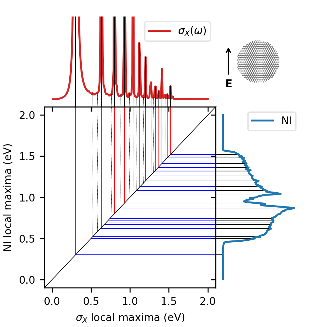
Figure 2: Correlation map between GD20 $\sigma_{X}(\omega)$ (top plot, red line) and NI (right plot, blue line) local maxima.

By varying the external field frequency, $\sigma_{X}$ shows a set of local maxima of different amplitudes. Since all calculations have been performed with a constant step of 0.01 eV, each PRF has an intrinsic error of 0.01 eV. Similar errors can also affect the relative intensity of the local maxima: the absorption peak is extremely sharp when $\tau$ is large, thus a small variation in frequency induces a large variation in intensity.

Similarly to $\sigma_{X}$, the NI plot is characterized by a distribution of local maxima, with the same intrinsic error of PRFs. From an inspection of fig. 2, a strong correlation between the two sets of local maximum points is observed, and this is especially true for the most significant maxima highlighted in fig. 2. This result is not surprising: from eq. 28 it is expected that a local maximum of $\sigma_{X}(\omega)$ is necessarily associated with a local maximum (in absolute value) of $\omega$FQ point charges. The charge densities associated with $\sigma_{X}(\omega)$ highlighted local maxima are plotted in fig. 3, and they clearly represent plasmon modes of increasing order. In fact, the number of nodes ($\text{N}_{\text{nodes}})$ is always odd for symmetry reason, and increases as frequency increases.Jackson (2007) Since the iterative procedure starts from the $\mathbf{q}_{0}=0$ vector, when the distance between the guess and the solution vectors increases, NI increases.

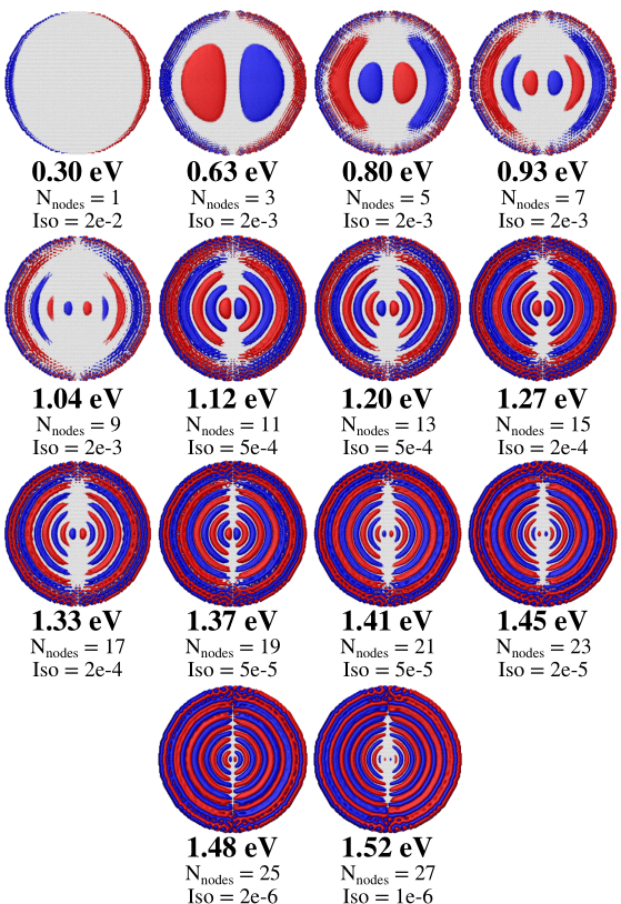
Figure 3: Graphical depiction of GD20 plasmon densities calculated at PRFs highlighted in fig. 2. The number of nodes ($\text{N}_{\text{nodes}}$) and the isovalue for each plasmon mode are also reported. Densities are obtained by superimposing the Gaussian density associated with each $\omega$FQ point charge. $\omega$FQ charges have been calculated through the GMRES algorithm by setting $\varepsilon_{F}=1.51$ eV, $\tau=170$ a.u. and $T=10^{-6}$.

Moving to the global trend of the NI (see fig. 2), the required number of iterations is small for the first PRF at $\omega=0.3$ eV, then the NI increases in the middle region of the spectrum and finally decreases. Two underlaying mechanisms may explain this peculiar trend. First, the lowest-order plasmon modes (e.g. the dipolar one at 0.3 eV) are strongly localized on the edge of the system (see fig. 3). Therefore a small number of large-valued point charges is involved in the excitation, but most charges are instead close to zero (e.g. those placed in the middle of the structure). By this, the guess vector $\mathbf{q}_{0}=0$ a.u. is a satisfactory starting point for the iterative procedure, and a small number of iterations is sufficient to obtain the solution vector. This is not true for the highest-order plasmon modes, that are instead delocalized all over the system (see fig. 3). In addition, the plasmonic response intensity (i.e. the point charges absolute value) strongly decreases when the excitation order increases (see fig. 2, top), because the number of nodes in the plasmon mode is larger. This is also evinced by the isovalue used to plot the densities in fig. 3, which decreases as the PRF increases. Therefore, the NI in correspondence to the highest order plasmon modes tends to decrease. The presence of low-amplitude local maxima, represented by dashed lines in fig. 2, top panel, can be attributed to numerical artifacts (see Fig. S3 in the SM).

The dependence of NI and $\sigma_{X}$ on $\tau$ and $\varepsilon_{F}$ is reported in figs. 4 and 6, respectively.

Figure 4: GD20 $\sigma_{X}(\omega)$ (top) and NI (bottom) as a function of $\tau$ (given in a.u.).

Focusing on the dependence on $\tau$ (fig. 4), we see that the PRF is not affected by this parameter, as it has been already reported in previous works.Giovannini et al. (2020) The main effect of the variation of $\tau$ is the shrinking of the excitation band shape, and the associated increase of intensity. In the energy region between 0.5 eV and 1.5 eV NI increases with $\tau$, and new local maxima in both $\sigma_{X}$ and NI at $\tau=680$ a.u. arise. These local maxima are associated to the high-order plasmon resonance modes identified in fig. 2 and represented in fig. 3.

The most relevant plasmon resonance mode is the dipolar excitation, because it is generally associated with the highest amplitude and the lowest PRF, which make it the most suitable for physical applications.Langer et al. (2020) A smaller value of $\tau$ can be adopted to achieve a reliable description of this excitation. In fig. 5, GD20 $\sigma_{X}$ calculated by setting $\tau=17000$ a.u. and $\tau=170$ a.u., and $\varepsilon_{F}=1.51$ eV are reported.

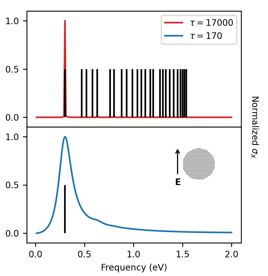
Figure 5: GD20 $\sigma_{X}$ calculated by setting $\tau=17000$ a.u. (top) or $\tau=170$ a.u. (bottom). Local maxima extrapolated from $\sigma_{X}$ are reported as black sticks.

Claerly, the first plasmon excitation with PRF=0.3 eV is the most intense for both $\tau$ values. For $\tau=170$ a.u., $\sigma_{X}$ is characterized by a single maximum since the reduction of the relaxation time induces also a proportional reduction of the plasmon excitation intensities.Giovannini et al. (2020) By this, we can conclude that $\tau=170$ a.u. can be chosen in order to reduce the computational cost of the iterative procedure, since we are mostly interested in the description of the dipolar excitation.

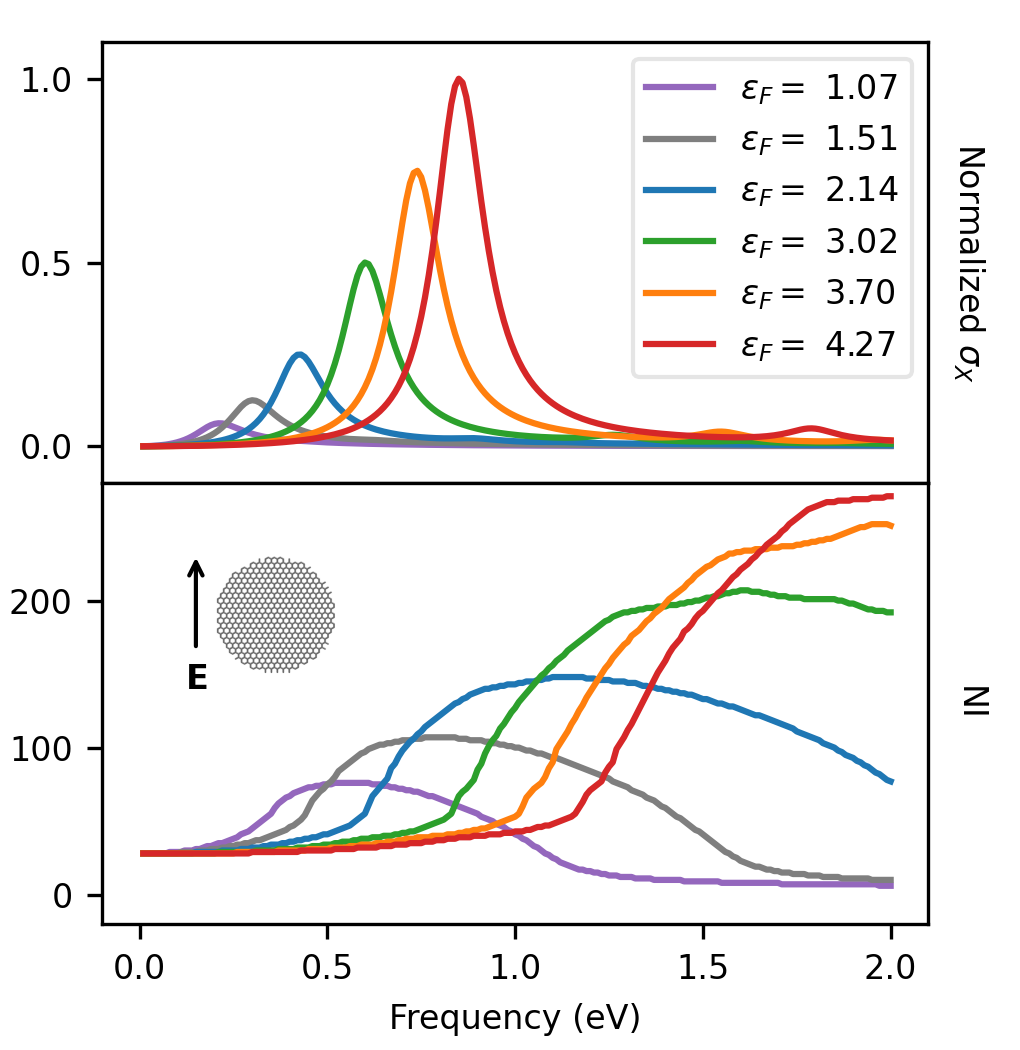
Figure 6: GD20 $\sigma_{X}$ (top) and NI (bottom) as a function of the Fermi energy $\varepsilon_{F}$ (given in eV).

The dependence of NI on $\varepsilon_{F}$ is reported in fig. 6. We see that the increase of $\varepsilon_{F}$ results in a blue shift of the PRF, and in the increase of the absorption intensity. In fact, a higher value of $\varepsilon_{F}$ is associated with an increase of $n_{\mathrm{2D}}$ (see eq. 7), because a higher fraction of $\pi$ electrons are involved in the excitation. The NI shows a similar trend, because the global maximum is blue shifted and the required number of iterations increases.

IV.2 Geometry

In this section, we investigate the dependence of NI on the geometry of the system. The same CNT and GD structures investigated in the previous section have been selected, for which we have varied the characteristic dimensions (see Fig. 1).

CNT. Table 1 reports the geometrical parameters of the selected structures.

	$L$ (nm)	Chiral numbers a	$d_{C}$ (nm)	Number of C atoms
CNT50	50	(8,12)	1.36	8208
CNT100	100			16416
CNT200	200			32832
CNT300	300			49248
CNT1	50	(8,12)	1.36	8208
CNT2		(16,24)	2.77	16416
CNT3		(24,36)	4.10	24624
CNT4		(32,48)	5.46	32832

^a The relation between the diameter $d_{C}$ and the chiral numbers $(n,m)$ is $d_{C}=\frac{b_{G}}{\pi}\sqrt{n^{2}+m^{2}+nm}$, where $b_{G}$ is the graphene lattice basis vector norm, i.e. 0.246 nmDresselhaus, Dresselhaus, and Saito (1998)

Table 1: Geometrical parameters of the studied CNT structures (see fig. 1(a) for their definition). The number of atoms for each structure is also given.

For each structure, the $\omega$FQ linear system in eq. 14 has been solved for 200 frequencies in the range between 0.0 eV and 2.0 eV with a constant step of 0.01 eV, by setting $\varepsilon_{F}=1.04$ eV and $\tau=170$ a.u., respectively. First, we comment the results obtained by fixing $d_{C}=1.36$ nm and by varying $L$ from 50 to 300 nm (see Table 1, top block). The data are shown in fig. 7 for both GMRES and QMR algorithms, in case the external field is aligned along the transversal (X) or longitudinal (Z) directions. We are then assuming that the two possible transversal directions (X and Y) provide the same polarization, even if all the considered CNTs are chiral. In fact, the differences in the plasmonic response along the two directions are negligible (see Fig. S4 in the SM).

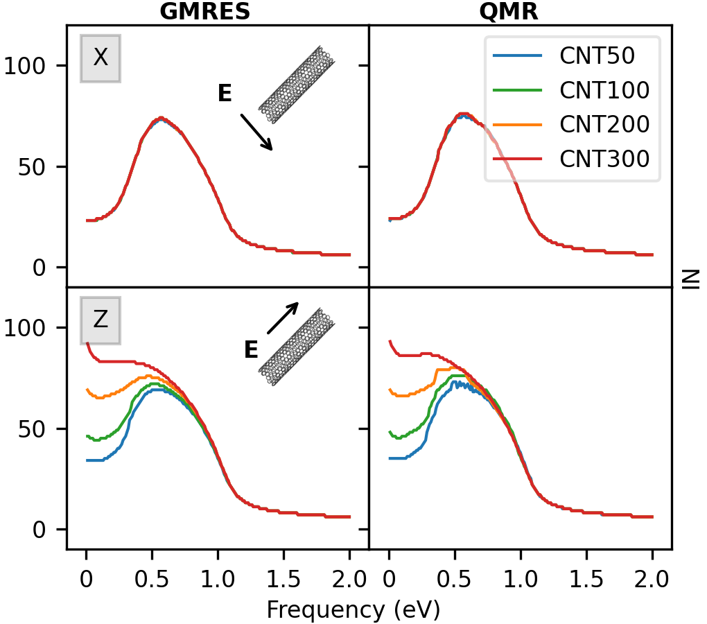
Figure 7: Convergence rate dependence on CNT length $L$ (see table 1) as calculated by using GMRES (left panel) and QMR (right panel). Both longitudinal (bottom) and transversal (top) polarizations of the external field are considered.

Figure 7, top panel, shows that the NI along the transversal direction is the same for all systems, because the diameter is kept constant. In case of longitudinal polarization, the number of iterative steps increases as the length of the system increases in the low energy region of the spectrum, for both GMRES and QMR. This is due to the fact that PRFs are red-shifted as $L$ increases approaching 0 eV (see Tab. S1 in the SM). The $z(\omega)$ factor in eq. 12 is therefore close to 0, and since the $\mathbf{A}$ matrix in eq. 14 is singular, the number of iterations increases due to increased ill-conditioning.

We now move to comment the results obtained by varying the CNT $d_{C}$, by keeping constant $L=50$ nm (see Table 1, bottom block). Computed GMRES and QMR NI for such systems are reported in fig. 8. Differently from the previous case, the NI trend does not show a strong dependence on $d_{C}$, for both transversal and longitudinal directions of the applied electric field. This is related to the fact that, although PRF energies are red-shifted as $d_{C}$ increases (along the X direction), the smallest PRF associated with the dipolar plasmon is far from 0 eV (0.37 eV for CNT4, see Tab. S1 in the SM). Therefore, in this case severe ill-conditioning is avoided and the NI remains almost constant.

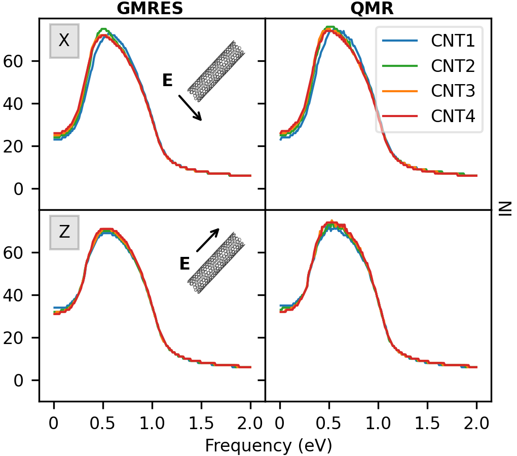
Figure 8: Convergence rate dependence on the CNT diameter $d_{C}$ (see table 1) as calculated by using GMRES (left panel) and QMR (right panel). Both longitudinal (bottom) and transversal (top) polarizations of the external field are reported.

As a final comment, we note that GMRES and QMR provide almost the same convergence rate. In particular, QMR NI is usually slightly higher than GMRES, thus confirming what has been observed in section III (see also Fig. S5 in the SM).

GD. Let us now focus on the NI calculated for four different GDs, obtained by varying the $d_{D}$ diameter (see fig. 1(b)). Geometrical parameters are reported in Table 2. The $\omega$FQ linear systems have been solved by setting the same parameters exploited in case of CNTs, and by imposing $\varepsilon_{F}=1.51$ eV. In this case, due to symmetry reason, the external electric field is polarized along one axis only.

ID	$d_{D}$ (nm)	Number of C atoms
GD20	20	11970
GD26	26	20058
GD32	32	30788
GD36	36	38974

Table 2: Geometrical parameters for the studied GDs (see fig. 1(b) for their definition). The number of atoms for each structure is also given.

For each structure, NI has been calculated for GMRES and QMR, and the results are reported in fig. 9. Interestingly, the NI presents a weak dependence on the $d_{D}$ diameter. In fact, the largest difference in the number of iterations is of about 10 between GD36 and GD20. However, GD36 has almost four times the atoms of GD20, thus demonstrating the favourable scalability of the two algorithms. We finally note that also in this case the PRFs are red-shifted as the size of the system increases (see Tab. S1 in the SM).

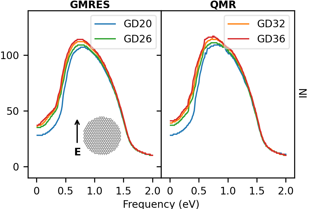
Figure 9: Convergence rate dependence on the GD diameter $d_{D}$ (see table 2), as calculated by using GMRES (left panel) and QMR (right panel).

IV.3 Algorithm parameters

We now move to consider the technical parameters associated with the iterative procedure, and how they affect the convergence rate. We first study the performance of GMRES($k$) (see section III), by taking as a reference system the CNT300 structure (see table 2) and exploiting the the same parameters used above for CNTs for solving the $\omega$FQ linear system. The iterative procedure has been performed by varying $k$ (between 20 and 80), and by keeping the threshold fixed to $T=10^{-6}$. Computed NI are reported in fig. 10, together with the corresponding results obtained with the full GMRES (F.G) algorithm (i.e. non-restarted). For X and Y polarizations, the reduction of the Krylov subspace does not affect the NI behaviour. On the contrary, for Z polarization GMRES($k$) and F.G. procedures yield different NI trends in the region between 0 and 0.2 eV. In fact, GMRES($k$) requires a larger number of iterations than F.G. version to reach convergence, independently of the dimension of the Krylov subspace $k$. This is once again due to singularities arising when PRF approaches to 0 eV, which yield ill-conditioning that is exacerbated in the restarted version of the algorithm. Such an explanation is corroborated by the evidence that the number of iterations required to reach convergence decreases by increasing the dimension of the Krylov subspace $k$. For each $k$, we also notice that GMRES($k$) is almost as efficient as the F.G. procedure in the remaining part of the spectrum. Therefore, in case the PRF is far from 0 eV, the same results can be obtained by using a cheaper iterative procedure in terms of memory requirements, because a smaller number of Krylov basis vectors have to be stored to build up the solution vector.

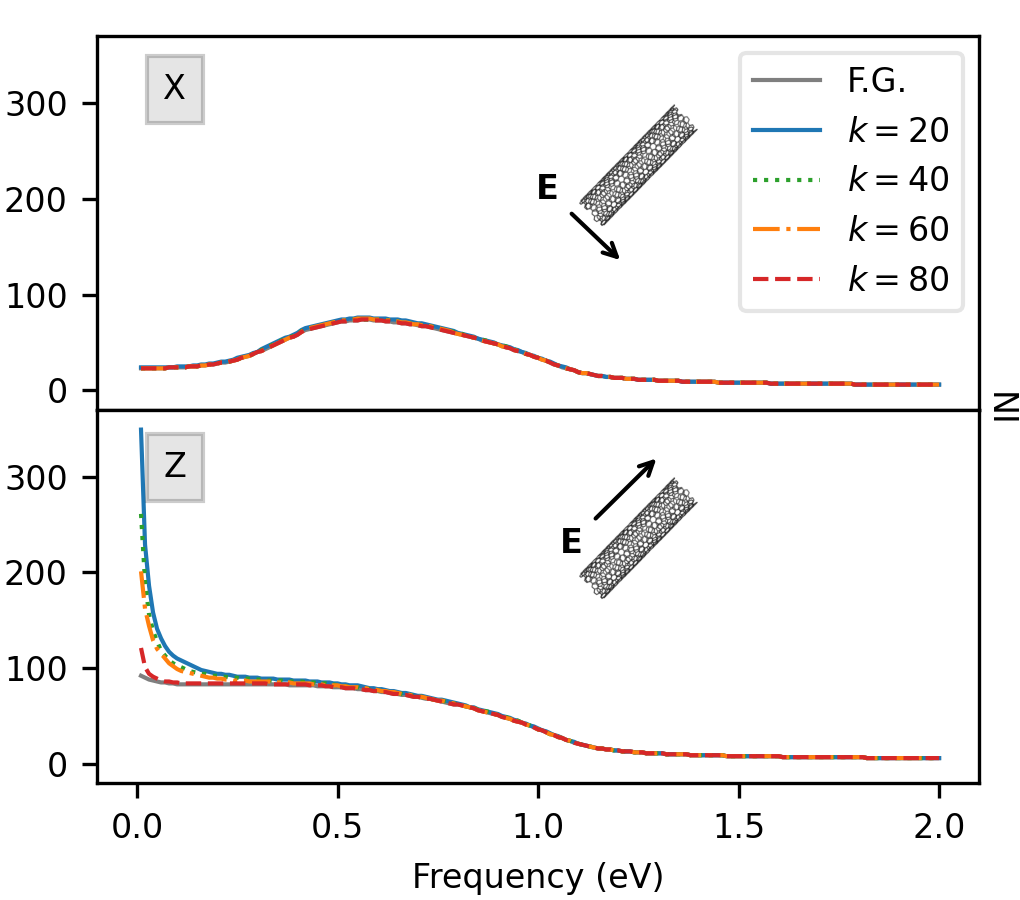
Figure 10: CNT300 NI dependence on the dimension of the Krlov subspace $k$ as calculated by using ($k$). The full GMRES (F.G.) values are also shown. Both longitudinal (bottom) and transversal (top) external field is considered.

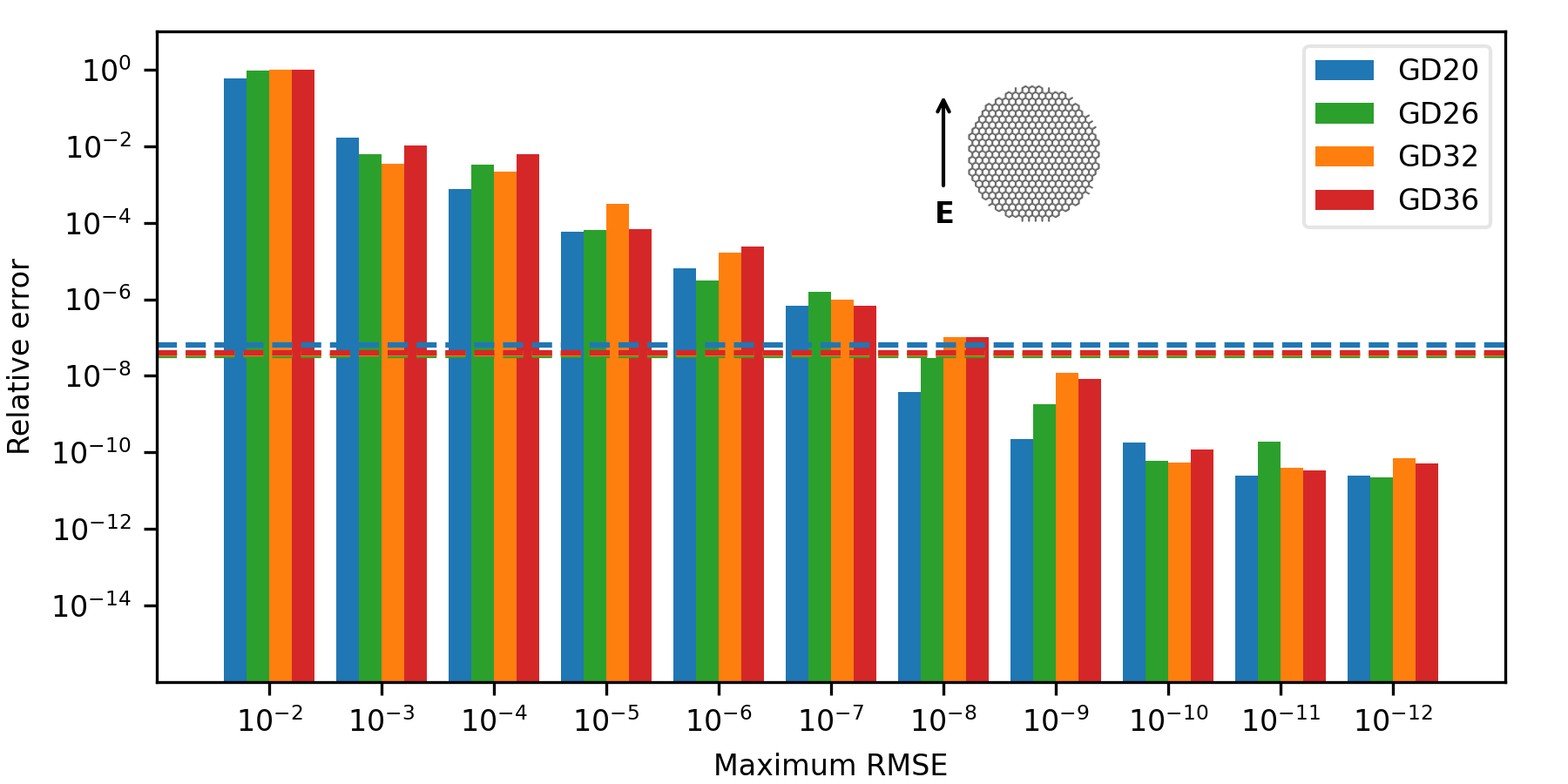
Figure 11: Average relative errors for GD20, GD26, GD32 and GD36 (see table 1) of the GMRES iterative solution with respect to LU factorization of the coefficient matrix at different choices of the RMSE introduced in eq. 33. Dashed lines indicate an approximate upper bound of the intrinsic precision associated with the inversion algorithm.

Another quantity that can strongly affect the NI is the threshold $T$ defined in eq. 27, which in all previous calculations has been fixed to $10^{-6}$. We notice however that $T$ is independent of the size of the system. Therefore, we can expect that the mean precision of the iterative solution, averaged for each charge, is higher when the number of atoms increases. In fact, eq. 27 can be rewritten as:

$$\left\|{\mathbf{r}_{k}}\right\|_{2}=\sqrt{\sum_{i=1}^{N}\left[R_{i}-((\mathbf{A}-z(\omega)\mathbf{I})\mathbf{q}_{k})_{i}\right]^{2}}<T.$$ (30)

If we assume that the absolute error is the same for each point charge, i.e. $R_{i}-((\mathbf{A}-z(\omega)\mathbf{I})\mathbf{q}_{k})_{i}=\delta q$, and we plug this approximation in eq. 30 we obtain:

$$\left\|{\mathbf{r}_{k}}\right\|_{2}\approx\sqrt{N}\delta q<T\quad\Rightarrow\quad\delta q<\frac{T}{\sqrt{N}},$$ (31)

Therefore, for a given threshold $T$ the absolute error on each charge decreases when the number of atoms $N$ increases.

In order to obtain a size-independent estimate of the accuracy of the iterative solution over all the $\omega$FQ charges, we can introduce the following definition of root mean squared error (RMSE):

$$\mathrm{RMSE}(\mathbf{x}_{k})=\frac{\left\|{\mathbf{R}-(\mathbf{A}-z(\omega)\mathbf{I})\mathbf{x}_{k}}\right\|_{2}}{\sqrt{N}}.$$ (32)

Then, we can define a new convergence criterion as:

$$\begin{split}\mathrm{RMSE}(\mathbf{x}_{k})<T\ \Rightarrow\ \left\|{\mathbf{R}-(\mathbf{A}-z(\omega)\mathbf{I})\mathbf{x}_{k}}\right\|_{2}<\sqrt{N}\cdot T,\end{split}$$ (33)

We can now investigate the accuracy of the iterative solution by adopting different RMSE thresholds. As a precision measure, we consider the longitudinal absorption cross section $\sigma_{X}$ calculated for a set of GDs (GD20, GD26, GD32, GD36 in table 2) applying an electric field with a polarization vector laying on the molecular plane. The linear system has been solved with both GMRES and a direct procedure, i.e. an LU factorization of the coefficient matrix.Golub and Van Loan (2013) For each selected RMSE value, the $\sigma_{X}$ relative error between GMRES and LU factorization averaged over all the considered frequencies (0.0 eV to 2.0 eV, with a step of 0.1 eV) has been calculated, and the results are graphically depicted in fig. 11. An approximate upper bound of the intrinsic precision associated with the factorization algorithm is also plotted (see section S1 in the SM).

It can be seen that the accuracy of the iterative solution for the different systems is almost constant for a specific RMSE value. In particular, by imposing RMSE$\leq 10^{-4}$, the correct order of magnitude obtained by using the LU solution can be recovered by the iterative procedure, i.e. the relative error is $\leq 10^{-1}$. To further demonstrate that the RMSE criterion is effectively size-independent, we performed the same analysis discussed above also for the CNT case (see Fig. S6 in the SM).

We finally move to discuss the computational time required by the different choices of the RMSE value. In particular, such an analysis has been performed on the four GDs reported in Table 2. The computational time required to solve the $\omega$FQ linear system for 20 frequencies in the range between 0.0 and 2.0 eV with a step of 0.1 eV are given in fig. 12 (raw data can be found in Tabs. S2-S5 in the SM). Both direct solution (LU factorization, see section S2 in the SM) and the full GMRES algorithm with different choices of RMSE have been considered. Notice that we are showing the computer time required by the solution of the $\omega$FQ linear system. This means that the coefficient matrix $\mathbf{A}$ (eq. 11) and right-hand side (eq. 13) construction are not taken into account, in order to allow for a direct comparison with the factorization algorithm. All calculations have been performed on a Xeon Gold 5120 (56 cores, 2.2 GHz) cluster node equipped with 256 GB RAM.

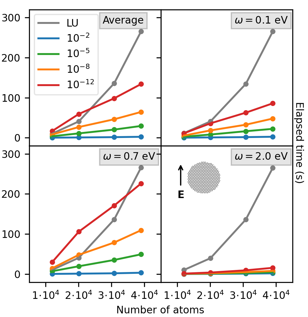
Figure 12: Computational time required to solve the $\omega$FQ linear system as a function of the number of atoms in GD structures. Average (top, left), $\omega=0.1$ eV (top, right), $\omega=0.7$ eV (bottom, left) and $\omega=2.0$ eV (bottom, right).

In fig. 12, the average computational time is reported (top, left panel) together with the time required to solve the $\omega$FQ linear system for three selected frequencies, i.e. 0.1 (lower bound), 0.7 and 2.0 eV (upper bound). $\omega=0.7$ eV has been chosen because it corresponds to the maximum number of iterations required by full GMRES to converge (see also fig. 9). Figure 12 clearly shows that the direct solution through LU factorization and the GMRES iterative procedure intrinsically differ in terms of the scaling with the dimension of the linear system (i.e. the number of atoms). In fact, the former has a complexity of $O(N^{3})$ while the latter scales as $O(N^{2})$. Such a difference is highlighted by the computational times in fig. 12: the increase of the computational time for the direct solution (gray line) is larger with respect to the iterative procedure when the number of atoms increases, independently of the RMSE value exploited in the GMRES algorithm. Also, we note that, differently from the LU-based algorithm, the computational time required by the iterative method is not constant across the frequency range. This can be explained by the fact that the number of iterations required to converge to the solution depends on the external frequency (see also fig. 9). Finally, we remark that even at 0.7 eV GMRES is more efficient than the inversion algorithm. In particular, a good compromise between accuracy and computational efficiency can be reached by using RMSE$=10^{-5}$, for which the computational time of the inversion solution can be reduced by a factor of 10 for the largest studied structure.

The computational time analysis has been performed also for the QMR algorithm (see section S2 and Tabs. S6-S9 in the SM). From an inspection of the numerical results, it emerges that, for a given RMSE, QMR requires roughly twice the computational time than GMRES. In fact, as it has been shown above, GMRES and QMR need a similar number of iterations to converge; however, for each iteration GMRES performs a single matrix-vector product, while QMR computes two matrix-vector products (one with the coefficient matrix, and one with the $\mathbf{D}$ matrix defined in eq. 3). Therefore, although the computational and memory costs of GMRES are not fixed during the iterative procedure, it overperforms QMR because of the lower number of matrix-vector products that are needed to build the Krylov subspace.

IV.4 Large systems

To finally demonstrate the robustness of the developed iterative methods to solve the $\omega$FQ linear system, we investigated the plasmonic response of real-size systems, composed of roughly one million atoms. When dealing with large-sized structures, two main issues arise. From the theoretical point of view, the quasi-static approximation on which $\omega$FQ equations are based could be no longer valid. From the technical point of view, when the number of atoms increases the storing of the $\omega$FQ matrix in physical memory can rapidly become unfeasible. Such a problem can be handled by adopting a matrix-free version of the GMRES algorithm, where the $\mathbf{A}$ matrix in eq. 14 is not explicitly built. In fact, the iterative algorithm only requires to calculate the matrix-vector product $\mathbf{Ax}$, which can be performed on-the-fly during the execution of the program. This means that at each iterative step $k$, the new Krylov basis vector is obtained as:

$$(\mathbf{x}_{k})_{i}=\sum_{j=1}^{N}(\mathbf{A}-z(\omega)\mathbf{I})_{ij}(\mathbf{x}_{k-1})_{j},$$ (34)

where the element $(i,j)$ of the matrix $\mathbf{A}-z(\omega)\mathbf{I}$ is calculated when required by the algorithm. On the other hand, each matrix element has to be calculated from scratch, therefore the on-the-fly version of GMRES would require larger computational time, without affecting the number of iterations. Nevertheless, the on-the-fly matrix-vector product can be efficiently calculated in a parallel environment and memory requirements are negligible with respect to the standard GMRES procedure, because only the iterative vectors should be kept in memory during the solution procedure.

To showcase the performance of GMRES when applied to large systems, we have selected three structures composed by roughly 1 million atoms: a carbon nanotube –CNT1M–, a graphene disk –GD1M– and a sodium nanorod –NR1M– (see Tab. S10 given in the SM, for geometrical parameters). The latter is genuinely different from the other two structures and has been selected to further demonstrate the reliability of the method to study the optical properties of metal nanostructures.

For each of the constructed structures, the longitudinal absorption cross sections and the NI have been calculated. We have set RMSE to $10^{-5}$, which has been proved in the previous section to be a good compromise between accuracy and the computational cost.

CNT1M. The calculations on CNT1M have been performed by applying an external field along the transversal and longitudinal directions, at 35 different frequencies in the range between 0.0 and 0.45 eV, by setting $\tau=170$ a.u. and $\varepsilon_{F}=1.03$ eV. The longitudinal absorption cross sections and the NI are reported in fig. 13. The transversal PRF is placed at about 0.38 eV, which is close to the value for CNT4, which has the same diameter (see table 1). The longitudinal PRF is instead placed at 0.02 eV, which is smaller than the value for CNT300, which has a length of 300 nm. This is not surprising because the PRF is red-shifted as the length of the system increases. The required number of iterations as a function of the external field frequency is reported in fig. 13. We note that the maximum number of iterations is 80, which is lower than what we have obtained for CNT300 (see section IV.2). This is due to the larger convergence threshold chosen for the iterative procedure; overall, a mean value of about 30 iterations is sufficient to reach the convergence. Since the number of iterations is modest, restarted GMRES has not been considered for such large systems. Moving on to discuss the computational time, our implementation permits to calculate about 4 matrix-vector product per hour, thus resulting in a total time of about 487 hours.

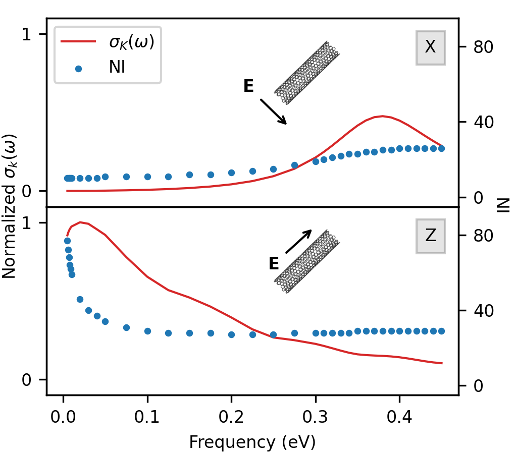
Figure 13: CNT1M $\sigma_{k}(\omega)$ (solid red line) and NI (blue dots). Both longitudinal ($k=Z$, bottom) and transversal ($k=X$, top) polarizations of the external field are reported. GMRES algorithm (RMSE = 10^-5).

GD1M. The $\omega$FQ linear system has been solved for GD1M with an external field polarization vector laying on the GD plane ($X$), at 15 different frequencies in the range between 0.05 and 0.19 eV with a constant step of 0.01 eV. We set $\tau=170$ a.u. and $\varepsilon_{F}=1.84$ eV. The computed $\sigma_{X}$ and NI are reported in fig. 14. The transversal dipolar PRF for this system lays at 0.12 eV, which is smaller than the values for the smallest GDs studied in the previous sections. The required number of iterations to reach convergence is about 30 for each external field frequency, i.e. smaller than what is required by GDs described in section IV.2. As it has been stated for CNT, this is mainly due to the setting of a larger RMSE threshold.

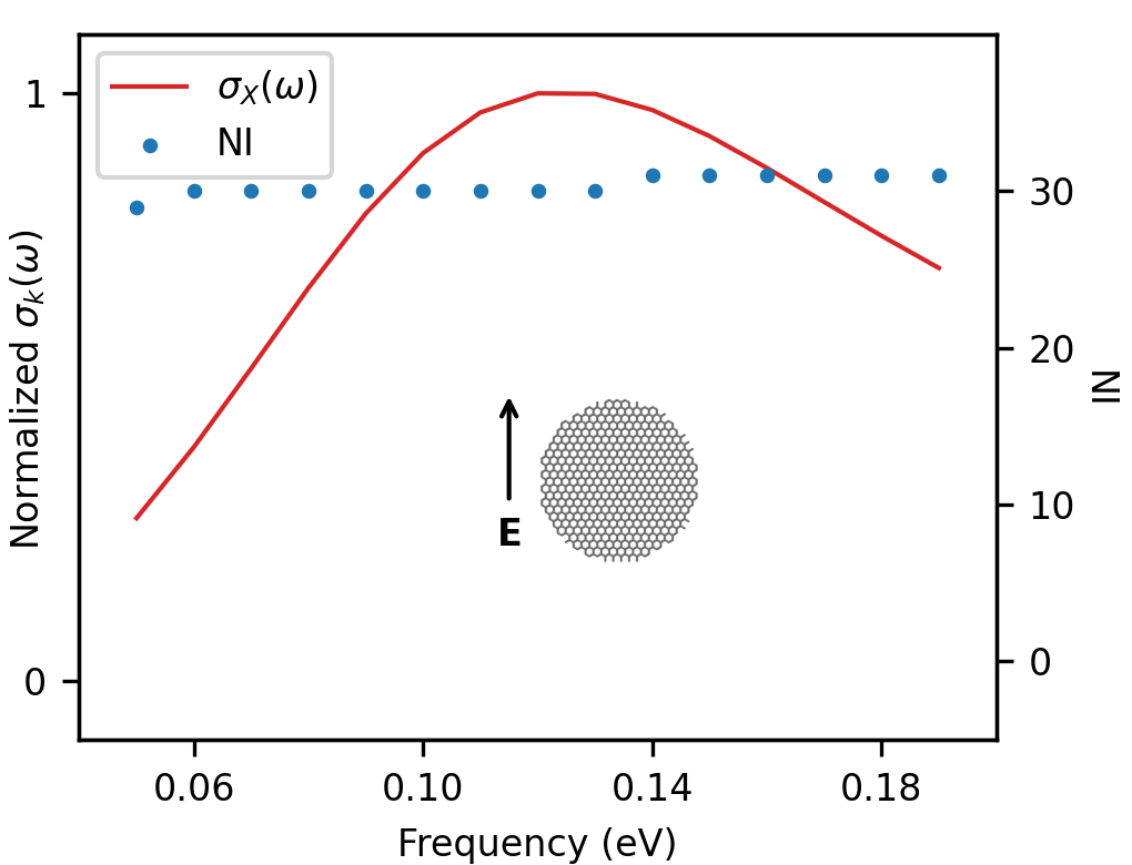
Figure 14: GD1M $\sigma_{X}(\omega)$ (solid red line) and NI (blue dots). GMRES algorithm (RMSE = 10^-5).

NR1M. Finally, we have calculated the plasmonic response of the NR1M system. This is a 3D nanostructure, therefore a general expression of the $\mathbf{K}^{\mathrm{tot}}$ matrix in terms of the 3D electron density $n_{0}$ (see eq. 5) needs to be exploited. All calculations have been performed with $\omega$FQ parameters for sodium reported in a previous work. Giovannini et al. (2019a) The linear system in eq. 14 has been solved for 24 frequencies in the range between 0.9 and 1.8 eV (unevenly distributed) with an external field aligned along the longitudinal ($Z$) direction. As for CNT1M and GD1M, the RMSE threshold was set to $10^{-5}$. The computed $\sigma_{Z}$ and the corresponding NI are reported in fig. 15.

The longitudinal PRF is placed at about 1.43 eV, which is blue shifted with respect to the longitudinal PRF of CNT1M, due to the fact that the electronic properties of the two materials are different. As for the previously studied carbon-based system, the value of the longitudinal PRF is red-shifted with respect to smaller sodium nanorods reported in a previous work.Giovannini et al. (2019a) This is once again due to the lighting rod effect discussed above. Similarly to previous cases, a mean value of about 30 iterations is sufficient to reach convergence.

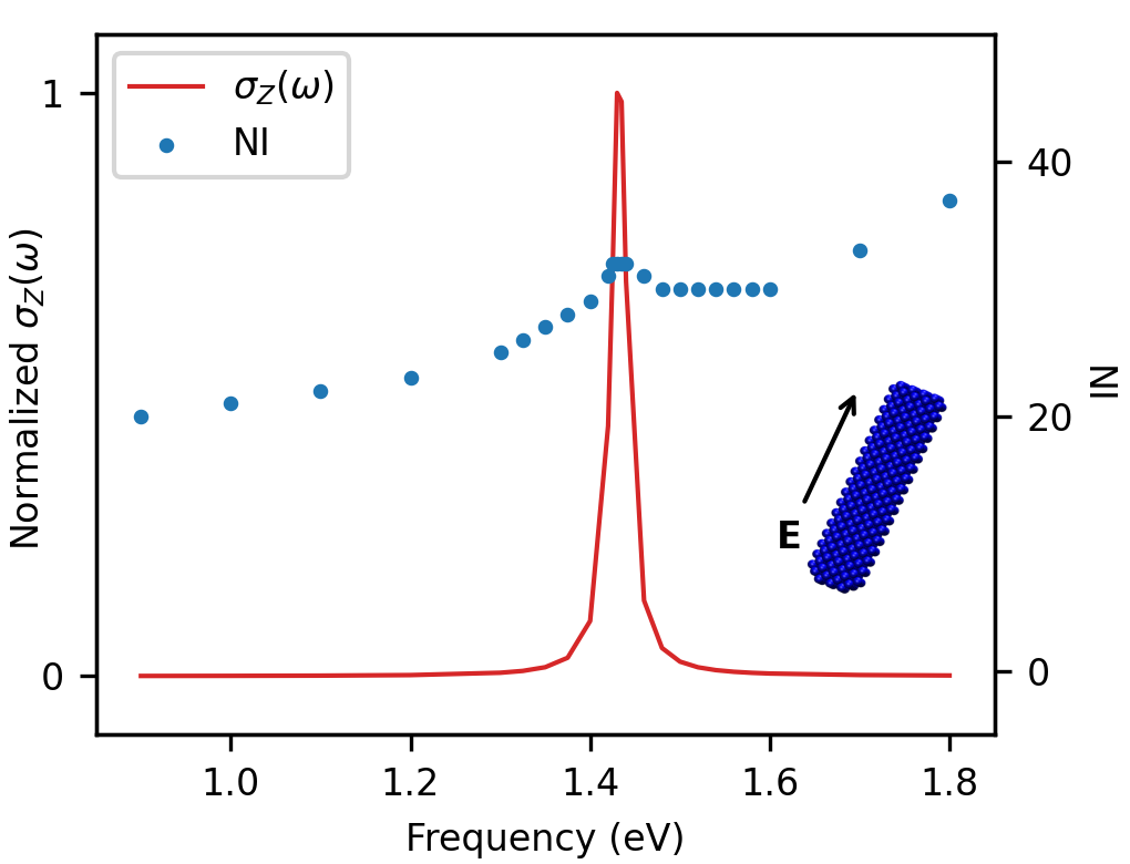
Figure 15: NR1M longitudinal $\sigma_{Z}(\omega)$ (solid red line) and NI (blue dots). GMRES algorithm (RMSE = 10^-5).

V Summary and Conclusions

In this paper, we have discussed how to substantially increase the applicability of classical, fully atomistic approaches to the calculation of the plasmonic properties of real-size nanostructures (carbon nanotubes, graphene-based materials and metal nanoparticles). State-of-the-art numerical iterative Krylov-based techniques, GMRES and QMR, have been specified to the recently developed fully atomistic $\omega$FQ model. For the studied structures, we have highlighted the dependence of the convergence rate on physical properties and parameters entering the definition of the model. It is worth remarking that a correlation between local maxima of the number of iterations and plasmon resonance frequencies is observed, showing that the convergence rate is particularly slowed down for high-order plasmons. Finally, on-the-fly implementation of GMRES has allowed the calculation of plasmon resonances of very large realistic nanostructures, composed of roughly one million atoms, which are not affordable by direct algorithms. We have also demonstrated the reliability of our implementation by showing that the required number of iterations to correctly describe the plasmon response of such large structures, is moderate.

The implemented iterative procedures are characterized by three main bottlenecks. On one hand, the number of matrix-vector products needed to build approximate solutions to the linear system is associated with a computational complexity of $O(N^{2})$. Linear scaling in matrix-vector products might be achieved through the fast multipole method (FMM)Rokhlin (1985); Engheta et al. (1985); Cipra (2000); Lipparini (2019), a numerical technique that can be adopted to build an approximation to the long-range electrostatic forces, which has already been applied to plasmonic substrates.Payton et al. (2014) Such an extension will allow to afford systems even larger than those studied in this work. However, in this case the quasi-static approximation on which $\omega$FQ relies, may be no longer valid. Therefore, retardation effects would need to be included in the model, similarly to what has already been proposed for continuum approaches.Waxenegger, Trügler, and Hohenester (2015); Hohenester (2014) A second bottleneck in our procedure is the lack of any preconditioning of the $\omega$FQ linear system. Different approaches may be exploited to solve dense complex linear systems, and they will be tested in future works for $\omega$FQ. Benzi (2002); Alléon, Benzi, and Giraud (1997); Chen (2005) Finally, in order to study the plasmonic properties of a given nanostructure along a specific spectral region, the $\omega$FQ linear system can be solved independently for each frequency. However, a change in frequency only affects the uniform diagonal shift of the coefficient matrix in eq. 14. Therefore, the shift-invariance property of the Krylov subspaces may be exploited by resorting to the so-called subspace recycling techniques.Sun et al. (2018); Soodhalter, de Sturler, and Kilmer (2020)

To conclude, another valuable application of $\omega$FQ is its potential applicability to theoretically describe Surface-Enhanced spectroscopies, either based on graphene-based substrates or metal nanoparticles.Langer et al. (2020); Ling et al. (2015) To this end, $\omega$FQ needs to be coupled with a quantum Hamiltonian describing the adsorbed moiety, in a QM/MM fashion.Morton and Jensen (2010, 2011); Payton et al. (2012, 2014); Chen et al. (2015) Such a further development is on-going in our group and will be the topic of future communications.

VI Acknowledgment

This work has received funding from the European Research Council (ERC) under the European Union’s Horizon 2020 research and innovation programme (grant agreement No. 818064).

Data Availability Statement The data that support the findings of this study are available from the corresponding author upon reasonable request.

References

- Liz-Marzán, Murphy, and Wang (2014) L. M. Liz-Marzán, C. J. Murphy, and J. Wang, “Nanoplasmonics,” Chem. Soc. Rev. 43, 3820–3822 (2014).
- Stockman (2011) M. I. Stockman, “Nanoplasmonics: past, present, and glimpse into future,” Opt. Express 19, 22029–22106 (2011).
- Maier (2007) S. A. Maier, Plasmonics: fundamentals and applications (Springer Science & Business Media, 2007).
- Chen et al. (2008) C.-F. Chen, S.-D. Tzeng, H.-Y. Chen, K.-J. Lin, and S. Gwo, “Tunable plasmonic response from alkanethiolate-stabilized gold nanoparticle superlattices: evidence of near-field coupling,” J. Am. Chem. Soc. 130, 824–826 (2008).
- Díez et al. (2009) I. Díez, M. Pusa, S. Kulmala, H. Jiang, A. Walther, A. S. Goldmann, A. H. Müller, O. Ikkala, and R. H. Ras, “Color tunability and electrochemiluminescence of silver nanoclusters,” Angew. Chem. Int. Edit. 48, 2122–2125 (2009).
- Stewart et al. (2008) M. E. Stewart, C. R. Anderton, L. B. Thompson, J. Maria, S. K. Gray, J. A. Rogers, and R. G. Nuzzo, “Nanostructured plasmonic sensors,” Chem. Rev. 108, 494–521 (2008).
- Lohse and Murphy (2013) S. E. Lohse and C. J. Murphy, “The quest for shape control: a history of gold nanorod synthesis,” Chem. Mater. 25, 1250–1261 (2013).
- Neto et al. (2009) A. C. Neto, F. Guinea, N. M. Peres, K. S. Novoselov, and A. K. Geim, “The electronic properties of graphene,” Rev. Mod. Phys. 81, 109 (2009).
- Cox, Silveiro, and García de Abajo (2016) J. D. Cox, I. Silveiro, and F. J. García de Abajo, “Quantum effects in the nonlinear response of graphene plasmons,” ACS Nano 10, 1995–2003 (2016).
- Jensen and Jensen (2008) L. L. Jensen and L. Jensen, “Electrostatic interaction model for the calculation of the polarizability of large noble metal nanoclusters,” J. Phys. Chem. C 112, 15697–15703 (2008).
- Jensen and Jensen (2009) L. L. Jensen and L. Jensen, “Atomistic electrodynamics model for optical properties of silver nanoclusters,” J. Phys. Chem. C 113, 15182–15190 (2009).
- Morton and Jensen (2010) S. M. Morton and L. Jensen, “A discrete interaction model/quantum mechanical method for describing response properties of molecules adsorbed on metal nanoparticles,” J. Chem. Phys. 133, 074103 (2010).
- Morton and Jensen (2011) S. M. Morton and L. Jensen, “A discrete interaction model/quantum mechanical method to describe the interaction of metal nanoparticles and molecular absorption,” J. Chem. Phys. 135, 134103 (2011).
- Payton et al. (2012) J. L. Payton, S. M. Morton, J. E. Moore, and L. Jensen, “A discrete interaction model/quantum mechanical method for simulating surface-enhanced Raman spectroscopy,” J. Chem. Phys. 136, 214103 (2012).
- Payton et al. (2014) J. L. Payton, S. M. Morton, J. E. Moore, and L. Jensen, “A hybrid atomistic electrodynamics–quantum mechanical approach for simulating surface-enhanced Raman scattering,” Accounts Chem. Res. 47, 88–99 (2014).
- Chen et al. (2015) X. Chen, J. E. Moore, M. Zekarias, and L. Jensen, “Atomistic electrodynamics simulations of bare and ligand-coated nanoparticles in the quantum size regime,” Nat. Commun. 6, 8921 (2015).
- Zakomirnyi et al. (2019) V. I. Zakomirnyi, Z. Rinkevicius, G. V. Baryshnikov, L. K. Sørensen, and H. Ågren, “Extended discrete interaction model: plasmonic excitations of silver nanoparticles,” J. Phys. Chem. C 123, 28867–28880 (2019).
- Li, Rinkevicius, and Ågren (2014) X. Li, Z. Rinkevicius, and H. Ågren, “Electronic circular dichroism of surface-adsorbed molecules by means of quantum mechanics capacitance molecular mechanics,” J. Phys. Chem. C 118, 5833–5840 (2014).
- Zakomirnyi et al. (2020) V. I. Zakomirnyi, I. L. Rasskazov, L. K. Sørensen, P. S. Carney, Z. Rinkevicius, and H. Ågren, “Plasmonic nano-shells: atomistic discrete interaction versus classic electrodynamics models,” Phys. Chem. Chem. Phys. 22, 13467–13473 (2020).
- Draine (1988) B. T. Draine, “The discrete-dipole approximation and its application to interstellar graphite grains,” Astrophys. J. 333, 848–872 (1988).
- Draine and Flatau (1994) B. T. Draine and P. J. Flatau, “Discrete-dipole approximation for scattering calculations,” J. Opt. Soc. Am. A 11, 1491–1499 (1994).
- Draine and Flatau (2013) B. T. Draine and P. J. Flatau, “User guide for the discrete dipole approximation code DDSCAT 7.3,” arXiv preprint arXiv:1305.6497 (2013).
- Sutradhar, Paulino, and Gray (2008) A. Sutradhar, G. Paulino, and L. J. Gray, Symmetric Galerkin boundary element method (Springer Science & Business Media, 2008).
- Hohenester and Trügler (2012) U. Hohenester and A. Trügler, “MNPBEM–A Matlab toolbox for the simulation of plasmonic nanoparticles,” Comput. Phys. Commun. 183, 370–381 (2012).
- Hohenester (2014) U. Hohenester, “Simulating electron energy loss spectroscopy with the MNPBEM toolbox,” Comput. Phys. Commun. 185, 1177–1187 (2014).
- Corni and Tomasi (2001) S. Corni and J. Tomasi, “Enhanced response properties of a chromophore physisorbed on a metal particle,” J. Chem. Phys. 114, 3739–3751 (2001).
- Giovannini et al. (2019a) T. Giovannini, M. Rosa, S. Corni, and C. Cappelli, “A classical picture of subnanometer junctions: an atomistic Drude approach to nanoplasmonics,” Nanoscale 11, 6004–6015 (2019a).
- Giovannini et al. (2020) T. Giovannini, L. Bonatti, M. Polini, and C. Cappelli, “Graphene plasmonics: Fully atomistic approach for realistic structures,” J. Phys. Chem. Lett. 11, 7595–7602 (2020).
- N’Tsame Guilengui et al. (2012) V. N’Tsame Guilengui, L. Cerutti, J.-B. Rodriguez, E. Tournié, and T. Taliercio, “Localized surface plasmon resonances in highly doped semiconductors nanostructures,” Appl. Phys. Lett. 101, 161113 (2012).
- Manjavacas, Nordlander, and García de Abajo (2012) A. Manjavacas, P. Nordlander, and F. J. García de Abajo, “Plasmon blockade in nanostructured graphene,” ACS Nano 6, 1724–1731 (2012).
- Anand et al. (2014) B. Anand, S. Krishnan, R. Podila, S. S. S. Sai, A. M. Rao, and R. Philip, “The role of defects in the nonlinear optical absorption behavior of carbon and ZnO nanostructures,” Phys. Chem. Chem. Phys. 16, 8168–8177 (2014).
- Bonatti et al. (2020) L. Bonatti, G. Gil, T. Giovannini, S. Corni, and C. Cappelli, “Plasmonic resonances of metal nanoparticles: Atomistic vs. continuum approaches,” Front. Chem. 8, 340 (2020).
- Van der Vorst (2003) H. A. Van der Vorst, Iterative Krylov methods for large linear systems, Vol. 13 (Cambridge University Press, 2003).
- Saad and Schultz (1986) Y. Saad and M. H. Schultz, “GMRES: A generalized minimal residual algorithm for solving nonsymmetric linear systems,” SIAM J. Sci. Stat. Comp. 7, 856–869 (1986).
- Freund and Nachtigal (1991) R. W. Freund and N. M. Nachtigal, “QMR: a quasi-minimal residual method for non-hermitian linear systems,” Numer. Math. 60, 315–339 (1991).
- Jackson (2007) J. D. Jackson, Classical electrodynamics (John Wiley & Sons, 2007).
- Giovannini, Egidi, and Cappelli (2020a) T. Giovannini, F. Egidi, and C. Cappelli, “Molecular spectroscopy of aqueous solutions: a theoretical perspective,” Chem. Soc. Rev. 49, 5664–5677 (2020a).
- Giovannini, Egidi, and Cappelli (2020b) T. Giovannini, F. Egidi, and C. Cappelli, “Theory and algorithms for chiroptical properties and spectroscopies of aqueous systems,” Phys. Chem. Chem. Phys. 22, 22864–22879 (2020b).
- Lipparini and Barone (2011) F. Lipparini and V. Barone, “Polarizable force fields and polarizable continuum model: a fluctuating charges/PCM approach. 1. theory and implementation,” J. Chem. Theory Comput. 7, 3711–3724 (2011).
- Giovannini et al. (2019b) T. Giovannini, A. Puglisi, M. Ambrosetti, and C. Cappelli, “Polarizable QM/MM approach with fluctuating charges and fluctuating dipoles: The QM/FQF model,” J. Chem. Theory Comput. 15, 2233–2245 (2019b).
- Mayer (2007) A. Mayer, “Formulation in terms of normalized propagators of a charge-dipole model enabling the calculation of the polarization properties of fullerenes and carbon nanotubes,” Phys. Rev. B 75, 045407 (2007).
- Rick, Stuart, and Berne (1994) S. W. Rick, S. J. Stuart, and B. J. Berne, “Dynamical fluctuating charge force fields: Application to liquid water,” J. Chem. Phys. 101, 6141–6156 (1994).
- De Abajo and Howie (2002) F. G. De Abajo and A. Howie, “Retarded field calculation of electron energy loss in inhomogeneous dielectrics,” Phys. Rev. B 65, 115418 (2002).
- Trügler et al. (2011) A. Trügler, J.-C. Tinguely, J. R. Krenn, A. Hohenau, and U. Hohenester, “Influence of surface roughness on the optical properties of plasmonic nanoparticles,” Phys. Rev. B 83, 081412 (2011).
- Fuchs (1975) R. Fuchs, “Theory of the optical properties of ionic crystal cubes,” Phys. Rev. B 11, 1732 (1975).
- Mayergoyz, Fredkin, and Zhang (2005) I. D. Mayergoyz, D. R. Fredkin, and Z. Zhang, “Electrostatic (plasmon) resonances in nanoparticles,” Phys. Rev. B 72, 155412 (2005).
- Fredkin and Mayergoyz (2003) D. Fredkin and I. Mayergoyz, “Resonant behavior of dielectric objects (electrostatic resonances),” Phys. Rev. Lett. 91, 253902 (2003).
- Saad (2003) Y. Saad, Iterative methods for sparse linear systems (SIAM, 2003).
- Meurant and Tebbens (2020) G. Meurant and J. D. Tebbens, Krylov Methods for Nonsymmetric Linear Systems: From Theory to Computations (Springer, 2020).
- Arnoldi (1951) W. E. Arnoldi, “The principle of minimized iterations in the solution of the matrix eigenvalue problem,” Q. Appl. Math. 9, 17–29 (1951).
- Golub and Van Loan (2013) G. H. Golub and C. F. Van Loan, Matrix computations, 4th Edition, Vol. 3 (JHU press, 2013).
- Joubert (1994) W. Joubert, “On the convergence behavior of the restarted GMRES algorithm for solving nonsymmetric linear systems,” Numer. Linear Algebr. 1, 427–447 (1994).
- Freund and Nachtigal (1994) R. W. Freund and N. M. Nachtigal, “An implementation of the QMR method based on coupled two-term recurrences,” SIAM J. Sci. Comput. 15, 313–337 (1994).
- Freund and Nachtigal (1995) R. W. Freund and N. M. Nachtigal, “Software for simplified Lanczos and QMR algorithms,” Appl. Numer. Math. 19, 319–341 (1995).
- Dagum and Menon (1998) L. Dagum and R. Menon, “OpenMP: an industry standard API for shared-memory programming,” IEEE Comput. Sci. Eng. 5, 46–55 (1998).
- Frayssé et al. (2003) V. Frayssé, L. Giraud, S. Gratton, and J. Langou, “A set of GMRES routines for real and complex arithmetics on high performance computers: Technical Report TR,” Tech. Rep. (PA/03/03, CERFACS, 2003) public domain software available on www.cerfacs/algor/Softs.
- Freund (1993) R. W. Freund, “A transpose-free quasi-minimal residual algorithm for non-hermitian linear systems,” SIAM J. Sci. Comput. 14, 470–482 (1993).
- García de Abajo (2014) F. J. García de Abajo, “Graphene plasmonics: challenges and opportunities,” ACS Photonics 1, 135–152 (2014).
- Thongrattanasiri, Manjavacas, and García de Abajo (2012) S. Thongrattanasiri, A. Manjavacas, and F. J. García de Abajo, “Quantum finite-size effects in graphene plasmons,” Acs Nano 6, 1766–1775 (2012).
- Langer et al. (2020) J. Langer, D. Jimenez de Aberasturi, J. Aizpurua, R. A. Alvarez-Puebla, B. Auguié, J. J. Baumberg, G. C. Bazan, S. E. J. Bell, A. Boisen, A. G. Brolo, J. Choo, D. Cialla-May, V. Deckert, L. Fabris, K. Faulds, F. J. García de Abajo, R. Goodacre, D. Graham, A. J. Haes, C. L. Haynes, C. Huck, T. Itoh, M. Käll, J. Kneipp, N. A. Kotov, H. Kuang, E. C. Le Ru, H. K. Lee, J.-F. Li, X. Y. Ling, S. A. Maier, T. Mayerhöfer, M. Moskovits, K. Murakoshi, J.-M. Nam, S. Nie, Y. Ozaki, I. Pastoriza-Santos, J. Perez-Juste, J. Popp, A. Pucci, S. Reich, B. Ren, G. C. Schatz, T. Shegai, S. Schlücker, L.-L. Tay, K. G. Thomas, Z.-Q. Tian, R. P. Van Duyne, T. Vo-Dinh, Y. Wang, K. A. Willets, C. Xu, H. Xu, Y. Xu, Y. S. Yamamoto, B. Zhao, and L. M. Liz-Marzán, “Present and future of surface-enhanced Raman scattering,” ACS Nano 14, 28–117 (2020).
- Dresselhaus, Dresselhaus, and Saito (1998) G. Dresselhaus, M. S. Dresselhaus, and R. Saito, Physical properties of carbon nanotubes (World scientific, 1998).
- Rokhlin (1985) V. Rokhlin, “Rapid solution of integral equations of classical potential theory,” J. Comput. Phys. 60, 187–207 (1985).
- Engheta et al. (1985) N. Engheta, W. D. Murphy, V. Rokhlin, and M. Vassiliou, “The fast multipole method for electromagnetic scattering computation,” IEEE T. Antenn. Propag. 40, 634–641 (1985).
- Cipra (2000) B. A. Cipra, “The best of the 20th century: Editors name top 10 algorithms,” SIAM News 33, 1–2 (2000).
- Lipparini (2019) F. Lipparini, “General linear scaling implementation of polarizable embedding schemes,” J. Chem. Theory Comput. 15, 4312–4317 (2019).
- Waxenegger, Trügler, and Hohenester (2015) J. Waxenegger, A. Trügler, and U. Hohenester, “Plasmonics simulations with the MNPBEM toolbox: Consideration of substrates and layer structures,” Comput. Phys. Commun. 193, 138–150 (2015).
- Benzi (2002) M. Benzi, “Preconditioning techniques for large linear systems: a survey,” J. Comput. Phys. 182, 418–477 (2002).
- Alléon, Benzi, and Giraud (1997) G. Alléon, M. Benzi, and L. Giraud, “Sparse approximate inverse preconditioning for dense linear systems arising in computational electromagnetics,” Numer. Algorithms 16, 1–15 (1997).
- Chen (2005) K. Chen, Matrix preconditioning techniques and applications, 19 (Cambridge University Press, 2005).
- Sun et al. (2018) D.-L. Sun, T.-Z. Huang, Y.-F. Jing, and B. Carpentieri, “A block gmres method with deflated restarting for solving linear systems with multiple shifts and multiple right-hand sides,” Numer. Linear Algebra Appl. 25, e2148 (2018).
- Soodhalter, de Sturler, and Kilmer (2020) K. M. Soodhalter, E. de Sturler, and M. E. Kilmer, “A survey of subspace recycling iterative methods,” GAMM-Mitteilungen 43, e202000016 (2020).
- Ling et al. (2015) X. Ling, S. Huang, S. Deng, N. Mao, J. Kong, M. S. Dresselhaus, and J. Zhang, “Lighting up the Raman signal of molecules in the vicinity of graphene related materials,” Accounts Chem. Res. 48, 1862–1870 (2015).