Deep Learning Phase Compression for MIMO CSI Feedback by Exploiting FDD Channel Reciprocity

Abstract

Large scale MIMO FDD systems are often hampered by bandwidth required to feedback downlink CSI. Previous works have made notable progresses in efficient CSI encoding and recovery by taking advantage of FDD uplink/downlink reciprocity between their CSI magnitudes. Such framework separately encodes CSI phase and magnitude. To further enhance feedback efficiency, we propose a new deep learning architecture for phase encoding based on limited CSI feedback and magnitude-aided information. Our contribution features a framework with a modified loss function to enable end-to-end joint optimization of CSI magnitude and phase recovery. Our test results show superior performance in indoor/outdoor scenarios.

I Introduction

Massive multiple-input multiple-output (MIMO) transceiver systems have demonstrated significant success in achieving high spectrum and energy efficiency for 5G and future wireless communication systems. These high achievable benefits require sufficiently accurate downlink (DL) channel state information (CSI) at the gNB (i.e., gNodeB). Frequency-division duplexing (FDD) systems, however, can only estimate DL CSI through feedback from UEs because DL and uplink (UL) channels occupy different frequency bands and may exhibit different channel characteristics. Since the feedback resource overhead grows proportionally with increasing MIMO size and spectrum, reducing CSI feedback overhead is vital to the widespread deployment of FDD MIMO systems. To improve feedback efficiency, previous works in [1, 2] developed a deep neural network with an autoencoder structure whose encoder at UEs and base stations, respectively for CSI compression and recovery. Related works and variants [3] have demonstrated performance advantages over traditional compressive sensing approaches.

Recent works have revealed the importance of exploiting correlated channel information such as UL CSI [4, 5], past CSI [6], and CSI adjacent UEs [7] for improving the accuracy of DL CSI recovery at base stations. In particular, important physical insights regarding FDD reciprocity, slow changes in propagation environment in time, and similar propagation conditions within short geographical distance, underscore respectively the strong spectral, temporal, and spatial correlations between magnitudes of different CSI in delay-angle (DA) domain. Since, side information from correlated CSI lowers the conditional entropy (uncertainty) of the DL CSI, their effective utilization reduces encoded feedback payload required from UEs [6].

Unlike the DA domain CSI magnitudes which tend to clearly exhibit strong temporal, spectral, and spatial correlations, CSI phases are very sensitive to changes in time, frequency, and location. To exploit the side CSI information, existing solutions have adopted dual feedback framework which separately encodes and recovers CSI phases from their corresponding magnitudes. These studies have utilized an isolated autoencoder to compress and recover the CSI magnitudes. For phase recovery, the basic principle in [4, 5, 7] is to expend more feedback resources (bandwidth) to encode the significant phases according to the corresponding magnitudes. For example, the authors in [7] designed a deep learning model with a magnitude-dependent polar-phase (MDPP) loss function to compress the significant CSI phases depending on the CSI magnitude.

Presently, these existing magnitude-dependent CSI feedback frameworks tend to train two learning models to encode and recover DL CSI magnitudes and phases, respectively. Intuitively, both CSI magnitudes and phases depend on the RF propagation environment including multipath delays, Doppler spread, bandwidth, and scatter distribution. CSI magnitude and phase encoding and recovery should be jointly instead of individually optimized. In fact, the structural sparsity of CSI phases and their joint distribution with the CSI magnitude are generally unknown and under explored.

In this work, we develop a deep learning based CSI feedback framework which jointly optimizes the magnitude and phase encoding. We propose a new loss function, namely sinusoidal magnitude-adjust phase error (SMAPE), that directly corresponds to the MSE of DL CSI recovery. Furthermore, we take advantage of the circular properties of CSI matrices in DA domain and propose a novel circularly convolutional neural network (C-CNN) layers proved to significantly enhance CSI compression efficiency and recovery performance.

II System Model

Without loss of generality, we consider a single-cell MIMO FDD link in which a gNB with $N_{b}$ antennas communicates with a single antenna UE. The OFDM signal spans $N_{f}$ DL subcarriers. The DL received signal of the $k$th subcarrier is

$$y_{\text{DL}}^{(k)}=\mathbf{h}_{\text{DL}}^{(k)H}\mathbf{w}_{\text{T}}^{(k)}x_{\text{DL}}^{(k)}+n_{\text{DL}}^{(k)},$$ (1)

where $(\cdot)^{H}$ denotes conjugate transpose. Here for the $k-$th subcarrier, $\mathbf{h}_{\text{DL}}^{(k)}\in\mathbb{C}^{N_{b}\times 1}$ denotes the CSI vector and $\mathbf{w}_{\text{T}}^{(k)}\in\mathbb{C}^{N_{b}\times 1}$ denotes the corresponding precoding vector whereas $x_{\text{DL}}^{(k)}\in\mathbb{C}$ and $n_{\text{DL}}^{(k)}\in\mathbb{C}$ denote the DL source signal and additive noise, respectively. With the same antennas, gNb receives UL signal

$$\mathbf{y}_{\text{UL}}^{(k)}=\mathbf{h}_{\text{UL}}^{(k)}x_{\text{UL}}^{(k)}+\mathbf{n}_{\text{UL}}^{(k)}\in\mathbb{C}^{N_{b}\times 1},$$ (2)

where subscript UL is used to denote uplink channel $\mathbf{h}_{\text{UL}}^{(k)}\in\mathbb{C}^{N_{b}\times 1}$, signal $x_{\text{UL}}^{(k)}$, and noise $\mathbf{n}_{\text{UL}}^{(k)}\in\mathbb{C}^{N_{b}\times 1}$. DL and UL channel vectors can be written as spatial-frequency CSI (SF-CSI) matrices ${\mathbf{H}}_{\text{DL}}^{\text{SF}}=[\mathbf{h}_{\text{DL}}^{(1)},...,\mathbf{h}_{\text{DL}}^{(N_{f})}]^{H}\in\mathbb{C}^{N_{f}\times N_{b}}$ and ${\mathbf{H}}_{\text{UL}}^{\text{SF}}=[\mathbf{h}_{\text{UL}}^{(1)},...,\mathbf{h}_{\text{UL}}^{(N_{f})}]^{H}\in\mathbb{C}^{N_{f}\times N_{b}}$, respectively. Typically in FDD systems, DL CSI ${\mathbf{H}}_{\text{DL}}^{\text{SF}}$ is estimated by UE for feedback to gNB. However, the number ($N_{f}\times N_{b}$) of unknowns in ${\mathbf{H}}_{\text{DL}}^{\text{SF}}$ occupies substantial feedback spectrum in large or massive MIMO systems. To exploit CSI sparsity to reduce feedback overhead, we apply IDFT $\mathbf{F}_{D}\in\mathbb{C}^{N_{f}\times N_{f}}$ and DFT $\mathbf{F}_{A}\in\mathbb{C}^{N_{b}\times N_{b}}$ on $\mathbf{H}^{\text{SF}}$ to generate DA domain CSI matrix

$$\mathbf{H}^{\text{DA}}=\mathbf{F}_{D}\mathbf{H}^{\text{SF}}\mathbf{F}_{A},$$ (3)

which demonstrates sparsity. Note that $\mathbf{H}^{\text{SF}}$ denotes either $\mathbf{H}^{\text{SF}}_{\text{UL}}$ or $\mathbf{H}^{\text{SF}}_{\text{UL}}$. Owing to limited multipath delay spread and limited number of scatters, most elements in $\mathbf{H}^{\text{DA}}$ are found to be near insignificant, except for the first $Q_{f}$ and the last $Q_{l}$ rows. Therefore, we shorten the CSI matrix $\mathbf{H}^{\text{DA}}$ in DA domain to $Q_{t}=Q_{f}+Q_{l}$ rows that contain sizable non-zero values and utilize $\mathbf{H}_{\text{DL}}$ and $\mathbf{H}_{\text{UL}}$ to denote the correspondingly truncated matrices of ${\mathbf{H}}_{\text{DL}}^{\text{DA}}$ and ${\mathbf{H}}_{\text{UL}}^{\text{DA}}$, respectively. For simplicity, we shall denote $\mathbf{H}_{\text{DL}}$ as $\mathbf{H}$ in the rest of this work except for cases when ambiguity may arise.

Subsequently, to further reduce the feedback overhead, the DL CSI matrix $\mathbf{H}$ is encoded at the UE and recovered by the gNB. The recovered DL CSI matrix can be expressed as

$$\widehat{\mathbf{H}}=f_{\text{de}}(f_{\text{en}}(\mathbf{H})),$$ (4)

where $f_{\text{en}}(\cdot)$ and $f_{\text{de}}(\cdot)$ denote encoding/decoding operations.

III Magnitude-aided CSI feedback Framework

Most deep-learning works on CSI compression leverage the success of real-valued deep learning network (DLN) in image processing by separating CSI matrices into real and imaginary parts that are analogous to image files [1, 2, 6], as shown in Fig. 1(a). Recent studies [4, 6, 7], however, uncovered the benefit of separately encoding magnitudes and phases of $\mathbf{H}$ instead in order to better exploit other correlated CSI magnitudes as auxiliary magnitude information (AMI). Such architecture, illustrated in Fig. 1(b), requires substantially lower feedback overhead for the magnitudes of $\mathbf{H}$ and allocate more feedback resources for phase feedback of $\mathbf{H}$.

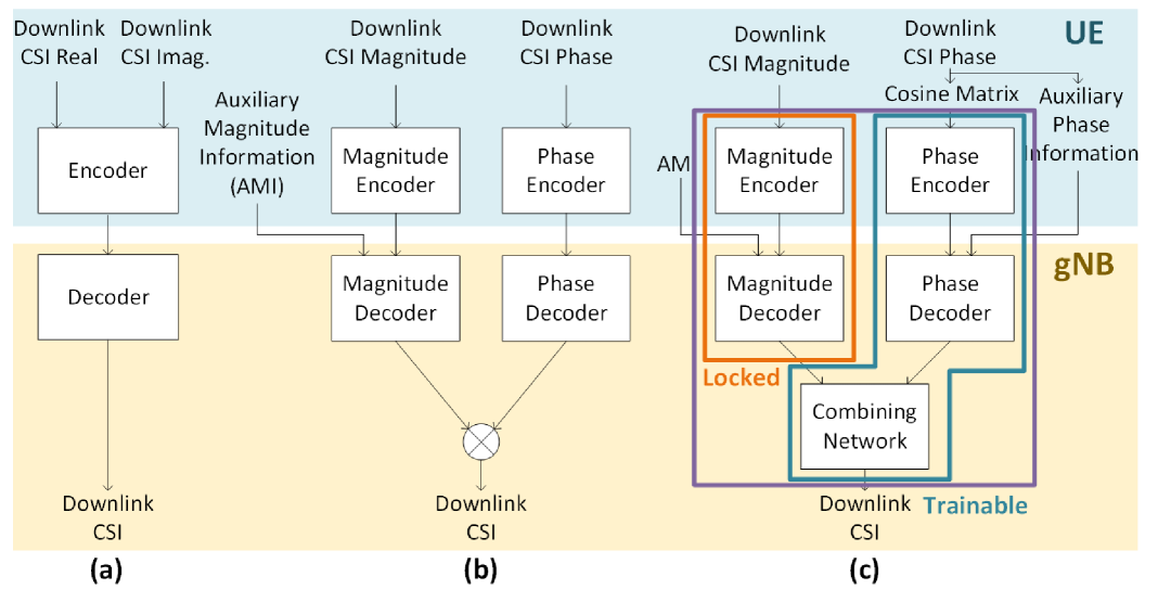
Figure 1: General network architecture. (a) Conventional CSI feedback framework, (b) conventional magnitude-aided CSI feedback framework, and (c) proposed magnitude-aided CSI feedback framework.

Fig. 1(c) illustrates our proposed new DLN framework, consisting of magnitude and phase branches. The gNB further contains a combining network to estimate the full CSI based on results from magnitude and phase decoders. We optimize encoders, decoders, and combining network jointly by minimizing a single loss function for end-to-end learning during offline training. Note that the magnitude branch can be independently optimized. To facilitate convergence [8], the training of the DLN has two stages. In stage-1, the CSI magnitude encoder/decoder branch is pre-trained for magnitude recovery. In stage-2, both the CSI phase branch and the combining network are optimized with the help of the magnitude branch, while the parameters of the magnitude branch are fixed.

III-A DualNet-MP

We now present a new DLN called DualNet-MP. As shown in Fig. 2, DualNet-MP splits each complex CSI matrix into

$$\mathbf{H}=|\mathbf{H}|\odot e^{j\measuredangle{\mathbf{H}}},$$

where $\odot$ represents Hadamard product. Denote the $(m,n)$-th entry of $\mathbf{H}$ as $\mathbf{H}_{m,n}=|\mathbf{H}_{m,n}|e^{j\measuredangle{\mathbf{H}_{m,n}}}$. The magnitude matrix $|\mathbf{H}|$ and consists of entries $|\mathbf{H}_{m,n}|$ and phase matrix $e^{j\measuredangle{\mathbf{H}}}$ consists of entries $e^{j\measuredangle{\mathbf{H}_{m,n}}}$.

Similar to [5], we forward the CSI magnitudes to the magnitude encoder network, including four $7\times 7$ circular convolutional layers with 16, 8, 4, 2 and 1 channels and activation functions. Given the circular characteristic of CSI matrices, we introduce circular convolutional layers to replace the traditional linear ones. Subsequently, a fully connected (FC) layer with $\left\lceil{\text{CR}_{\text{MAG}}Q_{t}N_{b}}\right\rceil$ elements is included for dimension reduction after reshaping. $\text{CR}_{\text{MAG}}$ denotes the magnitude compression ratio. The output of the FC layer is then fed into the quantization module, called the sum-of-sigmoid (SSQ) [5] to generate magnitude codewords for feedback.

At the gNB, a magnitude decoder uses magnitude codewords and available UL CSI magnitudes as AMI to jointly recover DL CSI magnitudes. The DL magnitude branch is first optimized by updating the network parameters $\Theta_{\text{MAG}}$

$${\mathop{\arg\min}_{\Theta_{\text{en,MAG}},\Theta_{\text{de,MAG}}}\left\{\mathinner{\!\left\lVert|\mathbf{\hat{H}}|-|\mathbf{H}|\right\rVert}^{2}_{\text{F}}\right\}}\\$$ (5)

to minimize the MSE of recovered MIMO CSI magnitude

$${|\mathbf{\hat{H}}|=f_{\text{de,MAG}}(f_{\text{en,MAG}}(|\mathbf{H}|,\Theta_{\text{en,MAG}}),\Theta_{\text{de,MAG}},\mathbf{H}_{\text{UL}}),}$$ (6)

in which $\Theta$ denotes DLN parameters and subscripts en, de, UL, and MAG of the $f(\cdot)$ denote the encoder, decoder, UL, and magnitude branch, respectively.

For CSI recovery of MIMO channels, we are only interested in their wrapped phases (i.e., $\measuredangle{\mathbf{H}}$). There is 1-to-1 relationship between a phase value $\phi$ and $\left(\cos(\phi),\mbox{sign}[\sin(\phi)]\right)$. For these reasons, we propose to form a ”cosine” matrix whose entries are cosines of entries from $\mathbf{H}$ denoted by

$$\mathbf{Cos}=\cos(\measuredangle{\mathbf{H}}).$$ (7a)

Let $$\mathbf{A}_{m,n}=\mbox{sign}[\sin[\measuredangle(\mathbf{H}_{m,n})]]$$. We also form a sign matrix

$${\mathbf{A}=\left[\mathbf{A}_{m,n}\right].}$$ (7b)

Thus $(\mathbf{Cos},\mathbf{A})$ uniquely determines $\measuredangle{\mathbf{H}}$.

Since $\mathbf{Cos}$ matrix is real, we can adopt a phase encoder similar to the magnitude encoder. Let $\text{CR}_{\text{PHA}}$ denotes the phase compression ratio. Each $\mathbf{Cos}$ generates a $\lceil\text{CR}_{\text{PHA}}Q_{t}N_{b}\rceil$-element codeword. Our DLN uses tanh activation function in each circular convolutional layer of the phase encoder to capture the underlying features of significant phases associated with large magnitudes. Upon completion of encoder training, the UE processes each CSI $\mathbf{H}$, and feeds back the CSI magnitude codeword $f_{\text{en,MAG}}(|\mathbf{H}|,\Theta_{\text{en,MAG}})$, the phase codeword $f_{\text{en,PHA}}(\mathbf{Cos},\Theta_{\text{en,PHA}})$ and the sign matrix $\mathbf{A}$ to gNB.

At the gNB receiver, the phase codeword $f_{\text{en,PHA}}(\mathbf{Cos},\Theta_{\text{en,PHA}})$ and the feedback sign matrix $\mathbf{A}$ are sent to the phase decoder with the tanh activation function as the last layer to constrain the entries of DL CSI cosine matrix $\widehat{\mathbf{Cos}}$ within $[-1,1]$. The magnitude codeword and side information are used by the magnitude decoder to obtain an estimated CSI magnitude matrix $|\widehat{\mathbf{H}}|$. Based on the relationship $\sin(\phi)=\mbox{sign}(\sin[\phi])\sqrt{1-\cos^{2}(\phi)}$, we form

$$\widehat{\mathbf{Sin}}=\mathbf{A}\odot(\mathbf{1}-\widehat{\mathbf{Cos}}\odot\widehat{\mathbf{Cos}})^{1/2}.$$

Therefore, we can directly generate a preliminary CSI estimate

$$\widehat{\mathbf{H}}=\left[|\widehat{\mathbf{H}}|\odot\widehat{\mathbf{Cos}},|\widehat{\mathbf{H}}|\odot\widehat{\mathbf{Sin}}\right]$$

from locally available $\widehat{\mathbf{Cos}}$, $\mathbf{A}$, $\widehat{|\mathbf{H}|}$. The combining network is trainable and can include two residual blocks containing four circular convolutional layers to refine the DL CSI matrix.

For end-to-end optimization, our training criterion relies on

$${\mathop{\text{minimize}}_{\Theta_{\text{en,PHA}},\Theta_{\text{de,PHA}},\Theta_{\text{C}}}\left\{\mathinner{\!\left\lVert\mathbf{\hat{H}}-\mathbf{H}\right\rVert}^{2}_{\text{F}}\right\},}\\$$ (8)

to optimize the parameters $\Theta_{\text{en,PHA}}$ of phase encoder $f_{\text{en,PHA}}$ and parameters $\Theta_{\text{de,PHA}}$ of phase decoder $f_{\text{en,PHA}}$ to estimate

$$\widehat{\mathbf{Cos}}=f_{\text{de,PHA}}(f_{\text{en,PHA}}(\mathbf{Cos},\Theta_{\text{en,PHA}}),\mathbf{A},\Theta_{\text{de,PHA}}).$$ (9)

Using the same loss function (8), we also train the combining network $f_{\text{C}}$ by optimizing parameters $\Theta_{\text{C}}$ to generate

$$\mathbf{\hat{H}}=f_{\text{C}}(|\widehat{\mathbf{H}}|,\widehat{\mathbf{Cos}},\Theta_{\text{C}}).$$ (10)

Since the training of the magnitude learning branch can be decoupled, our framework optimizes the entire architecture by minimizing the overall CSI MSE of (8). It is possible, however, to also partially incorporate the MSE of (8) to further refine the magnitude DLN branch by adopting a slower learning rate.

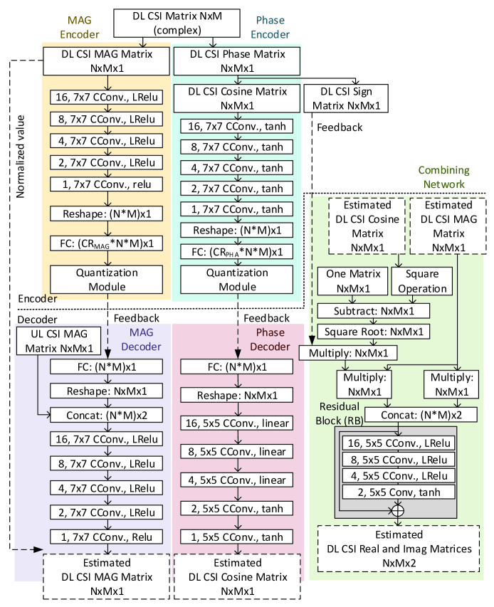
Figure 2: Network architecture of DualNet-MAG-PHA.

III-B Loss Function Redesign

Considering the MSE loss function, it may be intuitive to simply rewrite the loss function as follows:

$$Loss_{\text{0}}=\text{MSE}_{\text{CSI}}(\widehat{|\mathbf{H}|},\measuredangle{\hat{\mathbf{H}}})=\mathinner{\!\left\lVert\mathbf{H}-\mathbf{\hat{H}}\right\rVert}^{2}_{\text{F}}$$ (11)

$$=\mathinner{\!\left\lVert|\mathbf{H}|\odot\text{cos}(\measuredangle{\mathbf{H}})-|\hat{\mathbf{H}}|\odot\text{cos}(\measuredangle{\hat{\mathbf{H}}})\right\rVert}^{2}_{\text{F}}$$

$$+\mathinner{\!\left\lVert|\mathbf{H}|\odot\text{sin}(\measuredangle{\mathbf{H}})-|\hat{\mathbf{H}}|\odot\text{sin}(\measuredangle{\hat{\mathbf{H}}})\right\rVert}^{2}_{\text{F}}.$$

This means that $|\mathbf{H}|$ and $\measuredangle{\mathbf{H}}$ are used as encoder network input variables whereas their estimates are the decoder network output variables. However, the presence of infinitely many and shallow local minima of sinusoidal functions $\sin(\cdot)$ and $\cos(\cdot)$ often lead to training difficulties [9]. To overcome this problem, the authors in [7] recently proposed a weighted MDPP loss function

$$\text{MSE}_{\text{MDPP}}=\mathinner{\!\left\lVert|\measuredangle{\mathbf{H}}-\measuredangle{\mathbf{\hat{H}}}|{\odot}|\mathbf{H}|\right\rVert}^{2}_{\text{F}}\\$$ (12)

which still uses $|\mathbf{H}|$ and $\measuredangle{\mathbf{H}}$ as input and output variables. where $\measuredangle{\mathbf{H}}$ and $\measuredangle{\mathbf{\hat{H}}}$ denote the true and estimated phases, respectively. By weighting the original phase discrepancy with the true CSI magnitude, this new loss function helps capture the underlying features of the critical phases associated with CSI coefficents with dominant magnitudes. However, the loss function is not equivalent to our final goal for minimizing MSE of DL CSI. We now propose a reparamterization of the same MSE loss function during training. Instead of changing the loss function, we can overcome the training problem of directly parameterization in Eq. (17). Instead, recognizing that only the wrapped phases of $\measuredangle{\mathbf{H}}$ are of interest, we replace $\measuredangle{\mathbf{H}}$ with $\mathbf{Cos}$ and $\mathbf{A}$ via the following reparameterization:

$$\text{MSE}_{\text{SMAPE}}(\widehat{|\mathbf{H}|},\widehat{\mathbf{Cos}},\mathbf{A}) =\mathinner{\!\left\lVert\mathbf{H}-\mathbf{\hat{H}}\right\rVert}^{2}_{\text{F}}$$ (13)

$$=\mathinner{\!\left\lVert|\mathbf{H}|\odot\mathbf{Cos}-|\hat{\mathbf{H}}|\odot\widehat{\mathbf{Cos}}\right\rVert}^{2}_{\text{F}}$$

$$+\mathinner{\!\left\lVert|\mathbf{H}|\odot\mathbf{Sin}-|\hat{\mathbf{H}}|\odot\widehat{\mathbf{Sin}}\right\rVert}^{2}_{\text{F}},$$

where we have used the sign matrix $\mathbf{A}$ feedback to generate

$${\mathbf{Sin}} =\mathbf{A}\odot(\mathbf{1}-{\mathbf{Cos}}\odot{\mathbf{Cos}})^{1/2}$$ (14a)

$$\widehat{\mathbf{Sin}} =\mathbf{A}\odot(\mathbf{1}-\widehat{\mathbf{Cos}}\odot\widehat{\mathbf{Cos}})^{1/2}.$$ (14b)

This formulation saves about half the bandwidth by sending the sign matrix $\mathbf{A}$ without encoding matrix $\mathbf{Sin}$.

Moreover, the sparsity of $\mathbf{H}$ means that we only need to feed back partial entries of $\mathbf{A}$ associated with a swath of entries with dominant magnitudes. If we define a reduction ratio $R_{\text{s}}$ to further reduce feedback overhead. The total phase feedback overhead (in bits) is summarized as follows:

$$B_{\text{SMAPE}}=\text{CR}_{\text{PHA}}(K_{\text{PHA}}Q_{t}N_{b}+R_{\text{s}}Q_{t}N_{b})(\text{bits}),$$ (15)

where $K_{\text{PHA}}$ denotes the number of encoding bits for each entry of the compressed cosine matrix $f_{\text{en,PHA}}(\mathbf{Cos},\Theta_{\text{en,PHA}})$.

To summarize our training strategy of DualNet-MP, we use Eq. (5) as the loss function during the first training stage. In the second training stage, we used Eqs. (• ‣ IV-A) as the loss function to build an end-to-end learning architecture.

IV Experimental Evaluations

IV-A Experiment Setup

In our experiments, we let the UL and DL bandwidths be 20 MHz and the subcarrier number be $N_{f}$ = 1024. We consider both indoor and outdoor cases. We place the gNB with a height of 20 m at the center of a circular cell coverage with a radius of 20 m for indoor and 200 m for outdoor. The number of gNB antennas is $N_{b}=32$ whereas each UE has a single antenna. A half-wavelength inter-antenna spacing is considered. For each trained model, the number of epochs and batch size were set to 1,000 and 200, respectively. We generate two datasets each containing 100,000 random channels for both indoor and outdoor cases from two different channel models. 60,000 and 20,000 random channels are for training and validation. The remaining 20,000 random channels are test data for performance evaluation.

In the first (indoor) dataset, we used the COST 2100 [10] simulator and select the scenario IndoorHall at 5GHz to generate indoor channels at 5.1-GHz UL and 5.3-GHz DL with LOS paths. The antenna and band types are set as MIMO VLA omni and wideband, respectively. As for the outdoor dataset, we utilized QuaDRiGa simulator [11] with the scenario features of 3GPP 38.901 UMi. We considered the UMi scenario at 2 and 2.1 GHz of UL and DL bands, respectively, without LOS paths. The number of cluster paths was set as 13. The antenna type is set to omni. By DFT/IDFT operations and truncating described in Eqs. (3) and (4) of the revised manuscript, the resulting $32\times 32$ UL/DL CSI matrices in DA domain are obtained and be fed as the encoder input after proper processes.

The performance metric is the normalized MSE

$$\text{NMSE}=\frac{1}{D}\sum^{D}_{d=1}\mathinner{\!\left\lVert\widehat{\mathbf{H}}_{\text{DL},d}^{\text{SF}}-{\mathbf{H}}_{\text{DL},d}^{\text{SF}}\right\rVert}^{2}_{\text{F}}/\mathinner{\!\left\lVert{\mathbf{H}}_{\text{DL},d}^{\text{SF}}\right\rVert}^{2}_{\text{F}},$$ (16)

where the number $D$ and subscript $d$ denote the total number and index of channel realizations, respectively. Instead of evaluating the estimated DL CSI matrix $\widehat{\mathbf{H}}_{\text{DL}}$, we evaluate the estimated SFCSI matrix $\widehat{\mathbf{H}}_{\text{DL}}^{\text{SF}}$ that can be obtained by reversing the Fourier processing and padding zero matrix. Note that this NMSE includes both the errors caused by truncation at the encoder and the overall recovery error. Thus, it is practically more meaningful.

In the following section, we evaluate the performance of CSI recovery by adopting the proposed optimization method and encoder/decoder architecture. Thus, we trained DualNet-MP with the same core network design for magnitude recovery. However, we test different methods to reconstruct the CSI phases for two phase compression ratios of $\text{CR}_{\text{PHA}}=1/8$ and $1/16$ :

• SMAPE: the network architecture follows DualNet-MP as illustrated in Fig. 2 of the revised manuscript. The sign ratio $R_{\text{s}}$ varies between $[0.25,0.125]$ and we use $K_{\text{PHA}}=8$ bits for both $\text{CR}_{\text{PHA}}=\{1/8,1/16\}$. The loss function for phase reconstruction is given as follows:

  $$\text{MSE}_{\text{SMAPE}}(\widehat{|\mathbf{H}|},\widehat{\mathbf{Cos}},\mathbf{A}) =\mathinner{\!\left\lVert\mathbf{H}-\mathbf{\hat{H}}\right\rVert}^{2}_{\text{F}}$$

  $$=\mathinner{\!\left\lVert|\mathbf{H}|\odot\mathbf{Cos}-|\hat{\mathbf{H}}|\odot\widehat{\mathbf{Cos}}\right\rVert}^{2}_{\text{F}}$$

  $$+\mathinner{\!\left\lVert|\mathbf{H}|\odot\mathbf{Sin}-|\hat{\mathbf{H}}|\odot\widehat{\mathbf{Sin}}\right\rVert}^{2}_{\text{F}}.$$

• MDPQ [4]: the design assigns more encoding bits to encode the significant phases according the corresponding magnitudes. It assigns $[0,0,0,3,7]$ and $[0,0,0,0,5]$ bits for $\text{CR}_{\text{PHA}}=[1/8,1/16]$, respectively, to encode the CSI phases corresponding to $[0,0.5,0.7,0.8,0.9]$ of the cumulative distribution of CSI magnitude.

• MSE₀: instead of cosine, CSI phases are fed directly to the phase encoder. Both cosine and sine functions are appended as the final layer of the phase decoder to transform the decoded phase into cosine and sine, respectively, to recover the real and imaginary parts of CSI. We set $K_{\text{PHA}}$ to $8$ bits. The loss function for phase reconstruction is given as follows:

  $$\mbox{Loss}_{\text{0}}=\text{MSE}_{\text{CSI}}(\widehat{|\mathbf{H}|},\measuredangle{\hat{\mathbf{H}}})=\mathinner{\!\left\lVert\mathbf{H}-\mathbf{\hat{H}}\right\rVert}^{2}_{\text{F}}$$ (17)

  $$=\mathinner{\!\left\lVert|\mathbf{H}|\odot\text{cos}(\measuredangle{\mathbf{H}})-|\hat{\mathbf{H}}|\odot\text{cos}(\measuredangle{\hat{\mathbf{H}}})\right\rVert}^{2}_{\text{F}}$$

  $$+\mathinner{\!\left\lVert|\mathbf{H}|\odot\text{sin}(\measuredangle{\mathbf{H}})-|\hat{\mathbf{H}}|\odot\text{sin}(\measuredangle{\hat{\mathbf{H}}})\right\rVert}^{2}_{\text{F}}.$$

• MDPP [7]: we reuse the loss function Eq.(18) with the same network architecture. We set $K_{\text{PHA}}$ to $10$ bits.

  $$\text{MSE}_{\text{MDPP}}=\mathinner{\!\left\lVert|\measuredangle{\mathbf{H}}-\measuredangle{\mathbf{\hat{H}}}|{\odot}|\mathbf{H}|\right\rVert}^{2}_{\text{F}}\\$$ (18)

IV-B Different Phase Compression Designs

To demonstrate the superiority of the proposed SMAPE loss function, we applied different phase reconstruction approaches to DualNet-MP for different phase compression ratios $\text{CR}_{\text{PHA}}$. Figs. 3 (a) and (b) show the NMSE performance of different approaches under indoor and outdoor scenarios, respectively, at different compression ratios. As expected, DaulNet-MP encounters training difficulties when using the simple loss function $Loss_{0}$. By adopting MDPP loss functions, DualNet-MP performs much better than the simple loss function $Loss_{0}$. Although DualNet-MP appears to be better when using MDPQ instead of MDPP, encoding bit-assignment require careful tuning to achieve a satisfactory result. Finally, DualNet-MP based on the proposed SMAPE loss function achieves 4-dB performance improvement in terms of NMSE reduction for $\text{CR}_{\text{PHA}}$=1/8 at outdoor and 7-dB improvement for $\text{CR}_{\text{PHA}}$=1/8 at outdoor.

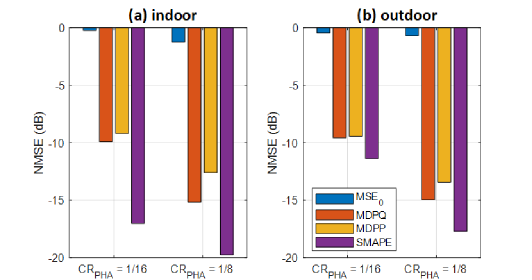
Figure 3: NMSE performance for different loss functions in (a) indoor and (b) outdoor scenarios.

IV-C Different Core Layer Designs

To investigate the appropriate core layer designs of DualNet-MP in order to efficiently extract the underlying features of CSI phases, we provide a performance evaluation using FC, linear convolutional, and circular convolutional layers, respectively, for the core network. Denoted respectively as DNN, CNN and C-CNN, these networks adopted SSQ [5] and binary-level quantization (BLQ) as the quantization module at the encoder. Denote that the DNN design follows the recent work [7]. We consider the phase compression ratio of $\text{CR}_{\text{PHA}}=1/8$. For SSQ, we assign $K_{\text{PHA}}=8$ bits for each codeword. That is, there are $\text{CR}_{\text{PHA}}Q_{t}N_{b}=128$ 8-bit codewords sent to the gNB. In contrast, there are $K_{\text{PHA}}\text{CR}_{\text{PHA}}Q_{t}N_{b}=1024$ 1-bit codewords when applying BLQ.

Figs. 4.(a) and (b) show the NMSE performance for the considered core layer designs. For both indoor and outdoor scenarios, DualNet-MP demonstrates superiority when adopting SSQ and C-CNN, which can be attributed to two possible reasons. Firstly, unlike BLQ, SSQ is differentiable such that it is easier to train. Secondly, there are many structural and circular features of CSI phases in the angle-delay domain that can be extracted better with the proposed structural changes.

In terms of storage and complexity of the proposed architecture, we note that C-CNN with only 826K parameters is considerably simpler than DNN of 11.6M parameters, using comparable floating point operations. Thus, the newly proposed DualNet-MP architecture combining SSQ and C-CNN provides both performance gain and cost benefits.

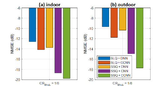
Figure 4: NMSE performance for different core layer designs in (a) indoor and (b) outdoor scenarios.

IV-D Accessment of FLOPs and parameter numbers

We evaluated the numbers of floating point operations (FLOPs) and parameters of DualNet-MP with different phase encoding approaches and core layer designs in Tables I and II, respectively. The comparison shows similarly complexity in terms of FLOPS. Since the complexity and storage issues are both crucial in the design of encoders deployed at UEs, we provide Table III to compare the encoder complexity between the proposed framework and two state-of-the-art alternatives.

TABLE I: FLOP and parameter numbers of DualNet-MP with different phase encoding schemes.

	MDPQ		$\text{MSE}_{\text{0}}$
$\text{CR}_{\text{PHA}}$	1/8,1/16		1/8	1/16
FLOPs	39.5M		77.2M	76.9M
Parameters	282.4K		825.9K	694.7K
	MDPP		SMAPE
$\text{CR}_{\text{PHA}}$	1/8	1/16	1/8	1/16
FLOPs	77.2M	79.6M	79.2M	78M
Parameters	825.9K	694.7K	826K	695.3K

TABLE II: FLOP and parameter numbers of DualNet-MP with different core layer designs when $\text{CR}_{\text{PHA}}=1/8$.

	DNN		C-CNN		CNN
Quantization Type	BLQ	SSQ	BLQ	SSQ	SSQ
FLOPs	118M	81.7M	82.8M	79.2M	79.2M
Parameters	34.2M	11.8M	2.6M	826K	826K

TABLE III: FLOP and parameter numbers at the encoders of DualNet-MP and state-of-the-art alternatives when $\text{CR}=1/8$.

Method	Parameters	FLOPs
CsiNet+	525K	1.86M
CoCsiNet	14.9M	39.1M
DualNet-MP	280K	38M

Since the FC layers are responsible for most of the parameters in many models, CoCsiNet requires the most parameters as it uses multiple FC layers at the encoder. Compared with CsiNet+, the proposed framework requires about half storage by separately encoding CSI phase and magnitude. To be specific, the FC layers require $(2048\times 256+256)$ and $2(1024\times 128+128)$ parameters at the encoders of CsiNet+ and DualNet-MP, respectively.

Often, convolutional layers contribute most FLOPs in a model due to the considerable number of two-dimensional convolution operations. However, DualNet-MP uses more convolutional layers at the encoder but still requires fewer FLOPs than CoCsiNet. Thus the proposed new architecture exhibits improvement in complexity reduction.

V Conclusions

This work presents a new deep-learning (DL) framework for large scale CSI estimation that leverages feedback compression and auxiliary CSI magnitude information in FDD systems. Utilizing vital domain knowledge in DL for CSI estimation to overcome known training issues, our new framework provides a novel loss function to enable efficient end-to-end learning and improves CSI recovery performance. We further exploit the circular characteristics of the underlying CSI in DA domain to propose an innovative circular convolution neural network (C-CNN). Our test results reveal significant improvement of overall CSI recovery performance for both indoor and outdoor scenarios and complexity reduction in comparison with a number of published alternative DL compression designs for MIMO CSI feedback.

References

- [1] C. Wen, W. Shih, and S. Jin, “Deep Learning for Massive MIMO CSI Feedback,” IEEE Wirel. Commun. Lett., vol. 7, no. 5, pp. 748–751, 2018.
- [2] J. Guo et al., “Convolutional Neural Network-Based Multiple-Rate Compressive Sensing for Massive MIMO CSI Feedback: Design, Simulation, and Analysis,” IEEE Trans. Wirel. Commun., vol. 19, no. 4, pp. 2827–2840, 2020.
- [3] Z. Qin et al., “Deep Learning in Physical Layer Communications,” IEEE Wirel. Commun., vol. 26, no. 2, pp. 93–99, 2019.
- [4] Z. Liu, L. Zhang, and Z. Ding, “Exploiting Bi-Directional Channel Reciprocity in Deep Learning for Low Rate Massive MIMO CSI Feedback,” IEEE Wirel. Commun. Lett., vol. 8, no. 3, pp. 889–892, 2019.
- [5] ——, “An Efficient Deep Learning Framework for Low Rate Massive MIMO CSI Reporting,” IEEE Trans. Commun., vol. 68, no. 8, pp. 4761–4772, 2020.
- [6] Z. Liu, M. Rosario, and Z. Ding, “A Markovian Model-Driven Deep Learning Framework for Massive MIMO CSI Feedback,” arXiv preprint arXiv:2009.09468, 2020.
- [7] J. Guo et al., “DL-based CSI Feedback and Cooperative Recovery in Massive MIMO,” arXiv preprint arXiv:2003.03303, 2020.
- [8] Y. Lin et al., “Learning-Based Phase Compression and Quantization for Massive MIMO CSI Feedback with Magnitude-Aided Information,” arXiv preprint arXiv:2103.00432, 2021.
- [9] G. Parascandolo, H. Huttunen, and T. Virtanen, “Taming the Waves: Sine as Activation Function in Deep Neural Networks,” 2017.
- [10] L. Liu et al., “The COST 2100 MIMO Channel Model,” IEEE Wirel. Commun., vol. 19, no. 6, pp. 92–99, 2012.
- [11] S. Jaeckel et al., “QuaDRiGa: A 3-D Multi-Cell Channel Model with Time Evolution for Enabling Virtual Field Trials,” IEEE Trans. Antennas and Propag., vol. 62, no. 6, pp. 3242–3256, 2014.