A Multi-Scale Method for Distributed Convex Optimization with Constraints

Abstract

This paper proposes a multi-scale method to design a continuous-time distributed algorithm for constrained convex optimization problems by using multi-agents with Markov switched network dynamics and noisy inter-agent communications. Unlike most previous work which mainly puts emphasis on dealing with fixed network topology, this paper tackles the challenging problem of investigating the joint effects of stochastic networks and the inter-agent communication noises on the distributed optimization dynamics, which has not been systemically studied in the past literature. Also, in sharp contrast to previous work in constrained optimization, we depart from the use of projected gradient flow which is non-smooth and hard to analyze; instead, we design a smooth optimization dynamics which leads to easier convergence analysis and more efficient numerical simulations. Moreover, the multi-scale method presented in this paper generalizes previously known distributed convex optimization algorithms from the fixed network topology to the switching case and the stochastic averaging obtained in this paper is a generalization of the existing deterministic averaging.

1 Introduction

The research of convex optimization by using multi-agent systems is a hot topic in recent decades. This problem typically takes the form of minimizing the sum of functions and is usually divided into subtasks of local optimizations, where each local optimization subtask is executed by one agent and the cooperation among these agents makes these local algorithms compute the optimal solution in a consensus way. Informally, convex optimization algorithms constructed in this way are usually termed as distributed convex optimization (DCO), which models a broad array of engineering and economic scenarios and finds numerous applications in diverse areas such as operations research, network flow optimization, control systems and signal processing; see nedic2009 ; nedic2010 ; nedic2015 ; boyd2011 ; feijer2010 ; duchi2012 ; ram2010 and references therein for more details.

Usually, DCO takes advantages of the consensus algorithms in multi-agent systems and gradient algorithms in convex optimization. The idea of combining them was proposed early in 1980s by Tsitsiklis et al. in tsitsiklis1986 and re-examined recently in the context of DCO in nedic2009 ; nedic2010 ; boyd2011 ; duchi2012 . Most DCO algorithms in the earlier development were discrete-time, with the distributed gradient descent strategy nedic2009 ; nedic2010 ; ram2010 being the most popular. Various extensions of the distributed gradient descent were then proposed, such as push-sum based approach nedic2015 , incremental gradient procedure ram2009 , proximal method parikh2013 , fast distributed gradient strategy jakovetic2014 ; qu2017 , and non-smooth analysis based technique zeng2017 , just to name a few. Additionally, using local gradients is rather slow and the community has moved towards using gradient estimation xin2018 ; qu2017 and stochastic gradient ram2010 ; yuan2016 . Further research directions were then followed by taking optimization constraints into consideration. Generally, DCO with constraints has proceeded along two research lines, namely projected gradient strategy and primal-dual scheme. The projected gradient strategy designed the optimization algorithms by projecting the gradient into the constraint set and extended it by including a consensus term ram2010 ; duchi2012 ; lou2016 . The primal-dual scheme introduced equality and inequality multipliers and designed for them extra dual dynamics charalamous2014 ; yi2015 ; zhu2011 in which a projection onto positive quadrant is usually included feijer2010 ; yi2015 ; charalamous2014 ; yamashita2020 so that the inequality-multiplier stays positive. Therefore, both research lines dealing with optimization constraints above are projection-dependent.

While projection-dependent algorithms were widely used in DCO, they require the optimization constraints to have a relatively simple form so that the projections can be computed analytically. To overcome this difficulty, this paper pursues a new method to design a novel DCO algorithm by avoiding projection. Our method is built on the primal-dual setup by introducing Lagrange multipliers. We modify the classical projection-based dynamics for the inequality-multiplier by utilizing the technique of mirror descent nemirovsky1983 ; raginsky2012 and design a projection-free multiplier-dynamics which is smooth. In conclusion, compared with most existing constrained DCO algorithms, our method avoids projection and thus reduces the difficulties of convergence analysis and iterative computation.

Aside from the difficulty associated with optimization constraints, the second challenge in DCO problem ties with stochastic networks and inter-communication noises. This challenge, together with optimization constraints, jointly make the DCO problem difficult to analyze, and therefore relatively few results were reported. Nedic nedic2015 considered DCO over deterministic and uniformly strongly connected time-varying networks without considering communication noises and optimization constraints; furthermore their algorithm needed a strong requirement that each node knows its out-degree at all times. The DCO problem with optimization constraints over time-varying graphs was investigated in xie2018 by using the epigraph form, but communication noises were not considered there. The work in lobel2011 also investigated the consensus-based DCO algorithm by using a random graph model where the communication link availability is described by a stochastic process, but leaving challenge issues of optimization constraints and communication noise untouched.

To tackle the above-mentioned difficulties and to contribute to the existing literature, this paper proposes a multi-scale method for constrained DCO problem over Markov switching networks under noisy communications. Unlike most existing DCO algorithms which are discrete-time, we study this problem in a continuous-time framework because the classical tools of Ito formula, backward Kolmogorov equation and ergodic theory in stochastic analysis can be used and the elegant Lyapunov argument in optimization theory feijer2010 can be invoked. Recently, we established in ni2016b a new technique of stochastic averaging (SA) for unconstraint DCO, where the idea of averaging was perviously explored by us to handle the switching networks of the multi-agent systems, with the deterministic version being presented in ni2013 ; ni2012 and the stochastic version in ni2016a . Compared with ni2016b , the present work considers a more general case of constrained optimization which is more challenge.

Although the SA viewpoint for multi-agent systems has been indicated in ni2016a , its theoretical clarification and design details were not provided there. In this paper, we generalize the SA principle in ni2016a to the DCO problem and propose a multi-scale based design procedure for the SA. We begin with the intuition behind our approach. Our multi-scale method borrows the idea of the slave principle in Synergetics haken1982 which was initially proposed by German physician Haken in 1970s. According to this principle, the system variables are classified into fast and slow ones, where the slow variables dominate the system evolution and characterize the ordering degree of the system. Therefore, it is necessary to eliminate the fast variables and obtain an equation for the slow variables only. This equation is called the principle equation and it can be viewed as an approximate description of the system. The method of eliminating the fast variables in physics is termed as Born-Oppenheimer approximation. In this paper, the continuous-time Markov chain characterizing the time-varying networks is regarded as the fast variable and, in contrast, the states of the optimization multi-agent system are considered as slow variables. To distinguish the fast and slow variables, two time-scales for them are introduced. In this paper, we propose a concrete scheme to eliminate the fast variable by resorting to the tool of multiscale analysis introduced by Pavliotis pavliotis and obtain an averaged SDE which acts as an approximation to the original switching stochastic differential equation (SDE). In this sense, the effect of network switching on optimization dynamics is eliminated, and thus the DCO under switching networks is, in fact, reduced to that under fixed case.

We mention two benefits of our multi-scale method. The first benefit in comparison with those dealing with random networks (see e. g. nedic2009 ,lobel2011 ) lies in its generalizability. The widely used DCO algorithms over random networks in nedic2009 ,lobel2011 built their analysis on the product theory of stochastic matrices (c.f. wolfowitz1963 ): the products of stochastic matrices converges to a rank one matrix (see Lemmas 4-7 in lobel2011 ). This theory was used to analyze the convergence of their optimization algorithm which is driven by a chain of stochastic matrices and an inhomogeneous gradient term (see Section V in lobel2011 ). However, due to technicalities involved, this method is hard to generalize to include optimization constraints or communication noises since otherwise the resulting matrices are not stochastic matrices. Our method does not have this limitation, instead it can treat the optimization constraints, communication noises and stochastic networks into a unified framework. As the second benefit, our method reduces the optimization algorithm in stochastic networks to that in fixed network (see Theorem 6.1) and establishes an approximation relationship between the two algorithms (see Theorem 6.2). Therefore, the SA method in this paper can help generalize existing DCO algorithms from fixed network to stochastic networks.

To sum up, the contributions of our paper are as follows. Firstly, this paper proposes a novel method of SA for the design and analysis of DCO problem, and addresses in a unified framework the challenge issues of the optimization constraints, communication noises and stochastic networks. Secondly, the SA method can help generalize some DCO algorithms from fixed network to switching case since it converts the latter to the former and establishes an approximation relationship between them. Thirdly, the DCO algorithm in this paper is projection-free and thus has the advantages of removing the difficulty of computing projection and rending the resulting optimization dynamics to be smooth so that algorithm analysis and simulation become relatively easy. Lastly, the multi-scale method used in this paper has the ability to generalize the averaging method from the deterministic case ni2013 ; ni2012 to the stochastic case in the present form, and it can also provide a theoretical justification for our original vision of SA for multi-agent systems ni2016a .

2 Preliminaries

A. Notations. For a vector $a$, its $i$-th component is denoted by $[a]_{i}$ or $a_{i}$. By $a\prec 0$ ($a\preccurlyeq 0$) we mean that each entry of $a$ is less than (less than or equal to) zero. Letting $a=(a_{1},\cdots,a_{n})^{T}\in\mathbb{R}^{n}$ and $b=(b_{1},\cdots,b_{n})^{T}\in\mathbb{R}^{n}$ , we define $a\odot\ b=(a_{1}b_{1},\cdots,a_{n}b_{n})^{T}$ and $a\oslash b\!=\!(a_{1}/b_{1},\cdots,a_{n}/b_{n})^{T}$. The notation $\mathbf{1}_{n}$ denotes an $n$-dimensional vector with each entry being $1$. We use $\mathbb{R}_{+}^{n}$ ($\mathbb{R}_{++}^{n}$) to denote the set of $n$-dimensional vectors with nonnegative (positive) components. For vectors $\alpha_{1},\cdots,\alpha_{m}$, the notation ${\rm col}\{\alpha_{i}\}_{i=1}^{m}$ denotes a new vector $(\alpha_{1}^{T},\cdots,\alpha_{m}^{T})^{T}$. For matrices $M_{1},\cdots,M_{m}$, we use ${\rm diag}\{M_{i}\}_{i=1}^{m}$ to denote block diagonal matrix with $i$-th block being $M_{i}$. The inner product between matrices is denoted as $A:B\!=\!{\rm tr}(A^{T}B)\!=\!\sum_{i,j}a_{ij}b_{ij}$, where ${\rm tr}$ denotes the matrix trace. For a map $g:\mathbb{R}^{n}\!\rightarrow\!\mathbb{R}^{m}$ which is differentiable at $x$, we use $\nabla g(x)$ to denote the matrix whose rows are the gradients of the corresponding entries in the vector $g(x)$.

B. Graph Theory. Consider a graph $\mathcal{G}=(\mathcal{V},\mathcal{E})$, where $\mathcal{V}=\{1,2,\cdots,N\}$ is the set of nodes representing $N$ agents and $\mathcal{E}\subset\mathcal{V}\times\mathcal{V}$ is the set of edges of the graph. The graph considered in this paper is undirected in the sense that the edges $(i,j)$ and $(j,i)$ in $\mathcal{E}$ are considered to be the same. The set of neighbors of node $i$ is denoted by $\mathscr{N}_{i}=\{j\in\mathcal{V}:(j,i)\in\mathcal{E},j\neq i\}$. We use the symbol $\cup$ to denote the graph union. We say that a collection of graphs is jointly connected if the union of its members is a connected graph. A collection of $\{\mathcal{G}_{1},\cdots,\mathcal{G}_{S}\}$ is jointly connected if and only if the matrix $\mathcal{L}_{1}+\cdots+\mathcal{L}_{S}$ has a simple zero eigenvalue, where $\mathcal{L}_{1},\cdots,\mathcal{L}_{S}$ are respectively the Laplacians of the graphs $\mathcal{G}_{1},\cdots,\mathcal{G}_{S}$.

3 Problem Formulation

Consider an optimization problem on a graph $\mathcal{G}=(\mathcal{V},\mathcal{E})$. Each agent $i\in\mathcal{V}$ has a local cost function $f_{i}(x)$ and a group of local inequality constraints $g_{ij}(x)\leq 0$, $j=1,\cdots,r_{i}$ and equality constraints $h_{ik}(x)=0,k=1,\cdots,s_{i}$, where $r_{i}$ and $s_{i}$ are nonnegative integers. If there is no constraints for agent $i$, one simply sets corresponding constraint functions to be zero. The total cost function of the network is given by sum of all local functions, and the optimization is to minimize the global cost function of the network while satisfying $N$ group of local constraints, given explicitly as follows,

$$\mathcal{P}:\left\{\begin{array}[]{llll}{\rm minimize}&&\tilde{f}(x)=\sum_{i=1}^{N}f_{i}(x),\\ {\rm subject~{}to}&&g_{i}(x)\preccurlyeq 0,\\ {\rm}&&h_{i}(x)=0,i=1,\cdots,N.\end{array}\right.$$ (4)

where $f_{i}:\mathbb{R}^{n}\rightarrow\mathbb{R}$, $g_{i}=(g_{i1},\cdots,g_{ir_{i}})^{T}:\mathbb{R}^{n}\rightarrow\mathbb{R}^{r_{i}}$, and $h_{i}=(h_{i1},\cdots,h_{is_{i}})^{T}:\mathbb{R}^{n}\rightarrow\mathbb{R}^{s_{i}}$ are respectively the local cost, inequality constraint and equality constraint on node $i$.

Let $x^{*}$ be an optimal solution, if exists, to the problem (4). If additional assumptions on the constraint functions, called constrained qualifications, are satisfied, then the following classical KKT conditions hold at the minimizer $x^{*}$: there exist $\lambda_{ij}^{*}$ and $\nu_{ij}^{*}$ such that, for $i=1,\cdots,N$,

$$g_{ij}(x^{*})\leq 0,j=1,\cdots,r_{i},$$ (5a)

$$h_{ij}(x^{*})=0,j=1,\cdots,s_{i},$$ (5b)

$$\lambda_{ij}^{*}\geq 0,j=1,\cdots,r_{i},$$ (5c)

$$\lambda_{ij}^{*}g_{ij}(x^{*})=0,j=1,\cdots,r_{i},$$ (5d)

$$\textstyle\sum\nolimits_{i=1}^{N}\!\nabla f_{i}(x^{*})\!+\!\sum\nolimits_{i=1}^{N}\!\sum\nolimits_{j=1}^{r_{i}}\lambda_{ij}^{*}\nabla g_{ij}(x^{*})$$

$$\hskip 36.98866pt+\textstyle\sum\nolimits_{i=1}^{N}\sum\nolimits_{j=1}^{s_{i}}\nu_{ij}^{*}\nabla h_{ij}(x^{*})=0.$$ (5e)

A widely used constrained qualification is the Slater’s constrained qualification (SQC): there exists $x\in\mathbb{R}^{n}$ such that $g_{i}(x)\!\prec\!0$ and $h_{i}(x)\!=\!0$ for $i=1,\cdots,N$. In other words, assuming SQC, “ $x^{*}$ solves ($\mathcal{P}$)” $\Rightarrow$ “ $\exists$ a set of $(\lambda_{ij}^{*},\nu_{ij}^{*})$ together with $x^{*}$ solving ($\mathcal{K}\mathcal{K}\mathcal{T}$)”. Furthermore, for convex problem, this implication is bidirectional. Refer to boyd2004 for details.

While SQC ensures the existence of multipliers satisfying ($\mathcal{K}\mathcal{K}\mathcal{T}$), it does not grantee uniqueness. Closely tied to this direction is the linear independent constraint qualification (LICQ), which is stronger than SCQ. Using $\nabla_{J_{i}}g_{i}(x^{*})$ to denote the submatrix of $\nabla g_{i}(x^{*})$ given by rows with indices in $J_{i}(x^{*})\!=\!\left\{j|g_{ij}\left(x^{*}\right)\!=\!0\right\}$, the LICQ is defined as

$$\operatorname{rank}\left[\begin{array}[]{lll}\nabla h_{i}(x^{*})\\ \nabla_{J_{i}}g_{i}(x^{*})\end{array}\right]=s_{i}+|J_{i}(x^{*})|,\quad i=1,\cdots,N,$$ (8)

here $|\cdot|$ denotes the set cardinality. By assuming LICQ, one obtains a result wachsmuth2013 on the existence and uniqueness of multipliers satisfying (5),

$$\scalebox{0.8}[1.0]{``$x^{*}$ solves ($\mathcal{P}$)''}\Rightarrow\scalebox{0.8}[1.0]{``$\exists$ a unique $(\lambda_{ij}^{*},\nu_{ij}^{*})$ together with $x^{*}$ solving ($\mathcal{K}\mathcal{K}\mathcal{T}$)''}.$$ (9)

This direction is bidirectional if the problem is convex. In what follows, we assume that $f_{i},g_{i},i=1,\cdots,N$ are convex and twice differentiable, and $h_{i},i=1,\cdots,N$ are affine, so that the optimization problem (4) is convex. Also, we assume the existence of optimal solutions without giving explicit conditions due to space limitation; interested readers can refer to boyd2004 . We further assume strict convexity on at least one function among $\{f_{1},\cdots,f_{i}\}$, so that there exists at most one global optimal solution to the problem (4). With these assumptions, the unique optimal solution is denoted by $x^{*}\in\mathbb{R}^{n}$ and the corresponding optimal value is denoted by $p^{*}=\tilde{f}(x^{*})$.

4 Distributed Optimization Dynamics

We use $N$ agents $\{1,\cdots,N\}$ to solve the convex optimization problem (4) in a distributed way. Each agent, say $i$, is a dynamical system with states $(x_{i}(t),\theta_{i}(t),\lambda_{i}(t),\nu_{i}(t))$ and communicates its estimate $x_{i}$ of the optimal solution $x^{*}$ to its neighboring agents. We consider the general case that the communication is corrupted by noises which lie in a filtered probability space $(\Omega,\mathcal{F},\mathbb{P},\{\mathcal{F}_{t}\}_{t\geq 0})$, where $\{\mathcal{F}_{t}\}_{t\geq 0}$ is a sequence of increasing $\sigma$-algebras with $\mathcal{F}_{\infty}\subset\mathcal{F}$ and $\mathcal{F}_{0}$ containing all the $\mathbb{P}$-null sets in $\mathcal{F}$. In more details, for any two neighbor agents $i,j$ with communication channel $(j,i)$ connecting them, the ideal relative information $(x_{j}\!-\!x_{i})$ transmitted in this channel is corrupted by state dependent noise $\sigma_{ji}\xi_{ji}(x_{j}-x_{i})$ with $\xi_{ji}(t)\in\mathbb{R}$ being independent standard white noises adapted to the filtration $\{\mathcal{F}_{t}|t\geq 0\}$ and $\sigma_{ji}\geq 0$ being noise intensity. This kind of noise indicates that the closer the agents are to each other, the smaller the noise intensities. The noise of this type is multiplicative in nature. While additive noise provides a natural intuition, multiplicative noise model also has its practical background. For example, it can model the impact of quantization error, as well as the effect of a fast-fading communication channel. Also, lossy communication induced noises and imperfect sample induced noises are all multiplicative noises. We also note that the issue of adopting multiplicative noise in inter-agent communication has been well explained in existing literatures (see for example references ni2013 , (li2014, , Remarks 1-2), carli2008 , wang2013 and references therein). By adopting this noise model, we design for each agent $i\in\{1,\cdots,N\}$ the following optimization dynamics

$$\dot{x}_{i}=c\sum_{j\in\mathscr{N}_{i}(t)}(1+\sigma_{ji}\xi_{ji})(x_{j}-x_{i})-\!\nabla f_{i}(x_{i})-\theta_{i}$$

$$\hskip 42.67912pt-\!\sum\nolimits_{j}^{r_{i}}\lambda_{ij}\nabla g_{ij}(x_{i})-\sum\nolimits_{j}^{s_{i}}\nu_{ij}\nabla h_{ij}(x_{i}),$$ (10a)

$$\dot{\theta}_{i}=-c\sum_{j\in\mathscr{N}_{i}(t)}(1\!+\!\sigma_{ji}\xi_{ji})(x_{j}-x_{i})$$ (10b)

$$\dot{\lambda}_{ij}=\frac{\lambda_{ij}}{1+\eta_{ij}\lambda_{ij}}g_{ij}(x_{i}),\hskip 14.22636ptj=1,\cdots,r_{i},$$ (10c)

$$\dot{\nu}_{ij}=h_{ij}(x_{i}),\hskip 56.9055ptj=1,\cdots,s_{i},$$ (10d)

where $x_{i},\theta_{i}\in\mathbb{R}^{n}$, $\lambda_{ij},\nu_{ij}\in\mathbb{R}$, $\eta_{ij}$ are positive parameters and $c>0$ is the coupling strength.

The equations (10a)-(10b) are motivated by (kia2015, , Eq. (3)), which however does not consider optimization constraints, communication noises, and more importantly time-varying network. This series of hard problems are tackled in our paper. The equation (10c) is motivated by (brunner2012, , Eq. (4)), but differs from brunner2012 since it is distributed by using $N$ agents on a network and considers the communication noises among agents and the stochastic networks. The dynamics (10d) can be obtained by maximizing $\Phi$ in (13) with respect to $\nu_{ij}$ via gradient ascent $\dot{\nu}_{ij}=\nabla_{\nu_{ij}}\Phi$.

The algorithm (10) is designed for time-varying networks. Assume that there are $S\!\in\!\mathbb{N}$ possible graphs $\{\mathcal{G}_{1},\cdots,\mathcal{G}_{S}\}$, among which the network structure is switched. We use a continuous-time Markov chain $\sigma:[0,\infty)\!\rightarrow\!\mathbb{S}\!:=\!\{1,\cdots,S\}$ to describe this switching. To analyze the stability of equation (10), we rewrite it into a switching SDE as (refer to Appendix A for detailed derivation and implicit definition of symbols in the equation below),

$$d\mbox{\boldmath$x$}\!=\![-c\boldsymbol{\mathcal{L}}_{\sigma(t)}\mbox{\boldmath$x$}\!-\!\mbox{\boldmath$\theta$}\!-\!\nabla F(\mbox{\boldmath$x$})\!-\!\boldsymbol{\lambda}\!\odot\!\nabla G(\mbox{\boldmath$x$})\!-\!\boldsymbol{\nu}\!\odot\!\nabla H(\mbox{\boldmath$x$})]dt\!+\!c\mathcal{M}_{\sigma(t)}d\mbox{\boldmath$w$},$$ (11a)

$$d\mbox{\boldmath$\theta$}=c\boldsymbol{\mathcal{L}}_{\sigma(t)}\mbox{\boldmath$x$}dt-c\mathcal{M}_{\sigma(t)}d\mbox{\boldmath$w$},$$ (11b)

$$d\boldsymbol{\lambda}=\left[\boldsymbol{\lambda}\oslash(\mathbf{1}+\boldsymbol{\eta}\odot\boldsymbol{\lambda})\right]\odot G(\mbox{\boldmath$x$})dt,$$ (11c)

$$d\boldsymbol{\nu}=H(\mbox{\boldmath$x$})dt.$$ (11d)

Note that we have assumed the existence and uniqueness of an optimal solution $x^{*}$. Defining $\mbox{\boldmath$x$}^{*}=\mathbf{1}_{N}\otimes x^{*}$, it follows from (9) that there is a unique pair of $(\mbox{\boldmath$\lambda$}^{*},\mbox{\boldmath$\nu$}^{*})$ satisfying (5), where $\mbox{\boldmath$\lambda$}^{*}$ and $\mbox{\boldmath$\nu$}^{*}$ are respectively stacked vectors of $\lambda_{ij}^{*}$ and $\nu_{ij}^{*}$ in (9). These give rise to another vector $\mbox{\boldmath$\theta$}^{*}$ defined by

$$\mbox{\boldmath$\theta$}^{*}\!+\!\nabla F(\mbox{\boldmath$x$}^{*})\!+\!\boldsymbol{\lambda}^{*}\!\odot\!\nabla G(\mbox{\boldmath$x$}^{*})\!+\!\boldsymbol{\nu}^{*}\!\odot\!\nabla H(\mbox{\boldmath$x$}^{*})=0,$$ (12)

Obviously, $(\mbox{\boldmath$x$}^{*},\mbox{\boldmath$\theta$}^{*},\mbox{\boldmath$\lambda$}^{*},\mbox{\boldmath$\nu$}^{*})$ satisfies (11) and consequently is an equilibrium of (11) (note that stochastic disturbances vanish at this equilibrium).

In the rest of this paper, we will utilize the averaging method used in ni2016a ; ni2016b to analyzed the stability of the equilibrium $(\mbox{\boldmath$x$}^{*},\mbox{\boldmath$\theta$}^{*},\mbox{\boldmath$\lambda$}^{*},\mbox{\boldmath$\nu$}^{*})$ for (11). The following assumptions are made:

Assumption 1

The LICQ defined in (8) is satisfied.

Assumption 2

The noise intensity $\sigma_{ij}$ has an upper bound $\sigma_{ij}\leq\kappa$ for some positive constant $\kappa$, where $i,j=1,\cdots,N$.

5 Distributed Optimization Under Fixed Network

In this section, we assume that the network is fixed, so that the time-varying graph Laplacian $\boldsymbol{\mathcal{L}}_{\sigma(t)}$ and the diffusion term $\mathcal{M}_{\sigma(t)}$ in the dynanmics (11) are replaced with fixed ones $\boldsymbol{\mathcal{L}}$ and $\mathcal{M}$, respectively. The following assumption is made:

Assumption 3

The coupling strength $c$ for fixed network satisfies $0<c<\frac{2}{3}\kappa^{-2}$.

The following theorem states that the trajectory of our optimization dynamics converges to its equilibrium $(\mbox{\boldmath$x$}^{*},\mbox{\boldmath$\theta$}^{*},\mbox{\boldmath$\lambda$}^{*},\mbox{\boldmath$\nu$}^{*})$ under appropriate conditions. While this result is obtained for fixed network, the multi-scale method developed in next section can transform the analysis of the optimization algorithm under switching networks to that under fixed one.

Theorem 5.1

For the constrained optimization problem (4), suppose there are $N$ agents with each agent dynamics given by (10), and they are connected across a fixed network (the graph Laplacian and diffusion term in (11) are now denoted as $\boldsymbol{\mathcal{L}}$ and $\mathcal{M}$ respectively). Under Assumptions 1-3 with $\kappa\leq\sqrt{\lambda^{\mathcal{L}}_{2}}/2$ with $\lambda^{\mathcal{L}}_{2}$ the smallest nonzero eigenvalue of the graph Laplacian $\mathcal{L}$, then for any trajectory of (11) with initial conditions $\lambda_{ij}(0)>0$ and $\sum_{i=1}^{N}\theta_{i}(0)=0$, one has $\lim_{t\rightarrow\infty}\|x_{i}(t)-x^{*}\|=0$ for $i=1,\cdots,N$ almost surely.

Proof We use the method of Lyapunov function to prove the stability, with the key to construct an appropriate Lyapunov function. Here we only give a proof skeleton, with more details being put in Appendices B, C, and D.

${\rm\mathbf{1}^{o}}$ Construct a Lyapunov candidate $V(\mbox{\boldmath$x$},\mbox{\boldmath$\theta$},\mbox{\boldmath$\lambda$},\mbox{\boldmath$\nu$})=V_{1}+V_{2}+V_{3}+V_{4}$ with

$$V_{1}=\frac{1}{2}\|\mbox{\boldmath$x$}-\mbox{\boldmath$x$}^{*}\|^{2}+\frac{1}{2}\|(\mbox{\boldmath$x$}-\mbox{\boldmath$x$}^{*})+(\mbox{\boldmath$\theta$}-\mbox{\boldmath$\theta$}^{*})\|^{2},$$

$$V_{2}=\frac{1}{2}\sum\nolimits_{i=1}^{N}\sum\nolimits_{j=1}^{r_{i}}\eta_{ij}(\lambda_{ij}-\lambda_{ij}^{*})^{2},$$

$$V_{3}=\sum\nolimits_{(i,j)\in\Omega}D_{\phi}(\lambda_{ij},\lambda_{ij}^{*})+\sum\nolimits_{(i,j)\notin\Omega}(\lambda_{ij}-\lambda_{ij}^{*})^{2},$$

$$V_{4}=\frac{1}{2}\sum\nolimits_{i=1}^{N}\sum\nolimits_{j=1}^{s_{i}}(\nu_{ij}-\nu_{ij}^{*})^{2},$$

where $\Omega\!=\!\{(i,j)|\lambda_{ij}^{*}\!\neq\!0\}$ and $D_{\phi}(\lambda_{ij},\lambda_{ij}^{*})\geq 0$ is the Bregman divergence between $\lambda_{ij}$ and $\lambda_{ij}^{*}$ with respect to $\phi(x)=x\ln x$ (refer to bregman1967 for the definition of Bregman divergence). Therefore, $V\!\geq\!0$, and also $V(\mbox{\boldmath$x$},\mbox{\boldmath$\theta$},\mbox{\boldmath$\lambda$},\mbox{\boldmath$\nu$})=0$ if and only if $(\mbox{\boldmath$x$},\mbox{\boldmath$\theta$},\mbox{\boldmath$\lambda$},\mbox{\boldmath$\nu$})\!=\!(\mbox{\boldmath$x$}^{*},\mbox{\boldmath$\theta$}^{*},\mbox{\boldmath$\lambda$}^{*},\mbox{\boldmath$\nu$}^{*})$.

${\rm\mathbf{2}^{o}}$ We now calculate the action of the operator $\mathcal{A}$ on the function $V$ (Recall that, for an SDE $dx=adt+bdw$, $\mathcal{A}V=\nabla V\cdot a+\frac{1}{2}{\rm tr}(b^{T}\nabla^{2}Vb)$). Defining an Lagrangian $\Phi:\mathbb{R}^{nN}\times\mathbb{R}^{nN}\times\mathbb{R}^{r}_{+}\times\mathbb{R}^{s}\rightarrow\mathbb{R}$ as

$$\Phi(\mbox{\boldmath$x$},\mbox{\boldmath$\theta$},\mbox{\boldmath$\lambda$},\mbox{\boldmath$\nu$})\!=\!\Psi\!+\!\sum_{i=1}^{N}\!\sum_{j=1}^{r_{i}}\!\lambda_{ij}g_{ij}(x_{i})\!+\!\!\sum_{i=1}^{N}\!\sum_{j=1}^{s_{i}}\!\nu_{ij}h_{ij}(x_{i})$$ (13)

with

$$\Psi(\mbox{\boldmath$x$},\mbox{\boldmath$\theta$})=\sum_{i=1}^{N}f_{i}(x_{i})+(\mbox{\boldmath$x$}-\mbox{\boldmath$x$}^{*})^{T}\mbox{\boldmath$\theta$}+\hbar\mbox{\boldmath$x$}^{T}\mbox{\boldmath$\mathcal{L}$}\mbox{\boldmath$x$},\quad\hbar=\frac{1}{2}(c-\frac{1}{2}c^{2}\kappa^{2}),$$ (14)

we can show in Appendix B that

$$\mathcal{A}V \leq\Phi(\mbox{\boldmath$x$}^{*},\mbox{\boldmath$\theta$},\mbox{\boldmath$\lambda$},\mbox{\boldmath$\nu$})-\Phi(\mbox{\boldmath$x$},\mbox{\boldmath$\theta$}^{*},\mbox{\boldmath$\lambda$}^{*},\mbox{\boldmath$\nu$}^{*})\!-\!(\hbar\lambda^{\mathcal{G}}_{2}\!-\!1)(\mbox{\boldmath$x$}\!-\!\mbox{\boldmath$x$}^{*})^{T}(\mbox{\boldmath$x$}\!-\!\mbox{\boldmath$x$}^{*}),$$ (15)

where $\lambda^{\mathcal{G}}_{2}$ is the smallest nonzero eigenvalue of the connected graph $\mathcal{G}$. Noting that $(x^{*},\mbox{\boldmath$\lambda$}^{*},\mbox{\boldmath$\nu$}^{*})$ satisfies (5), we show in Appendix C that the following saddle point condition holds

$$\Phi(\mbox{\boldmath$x$}^{*},\mbox{\boldmath$\theta$},\mbox{\boldmath$\lambda$},\mbox{\boldmath$\nu$})\!\leq\!\Phi(\mbox{\boldmath$x$}^{*},\mbox{\boldmath$\theta$}^{*},\mbox{\boldmath$\lambda$}^{*},\mbox{\boldmath$\nu$}^{*})\leq\Phi(\mbox{\boldmath$x$},\mbox{\boldmath$\theta$}^{*},\mbox{\boldmath$\lambda$}^{*},\mbox{\boldmath$\nu$}^{*}).$$ (16)

Therefore, $\mathcal{A}V\!\leq\!0$ if $\hbar\lambda^{\mathcal{G}}_{2}\!-\!1>0$, which is guaranteed by $\kappa\leq\scalebox{0.8}[0.7]{$\sqrt{\lambda_{2}^{\mathcal{G}}}$}/2$.

${\rm\mathbf{3}^{o}}$ Letting $\mathcal{A}V=0$, we show in Appendix D that $(\mbox{\boldmath$x$},\mbox{\boldmath$\theta$},\mbox{\boldmath$\lambda$},\mbox{\boldmath$\nu$})=(\mbox{\boldmath$x$}^{*},\mbox{\boldmath$\theta$}^{*},\mbox{\boldmath$\lambda$}^{*},\mbox{\boldmath$\nu$}^{*})$. The application of the stochastic version of the Lasalle’s invariance principle in mao1999 yields that the equilibrium $(\mbox{\boldmath$x$}^{*},\mbox{\boldmath$\theta$}^{*},\mbox{\boldmath$\lambda$}^{*},\mbox{\boldmath$\nu$}^{*})$ of system (10) is asymptotically stable almost surely. ∎

6 Multi-Scale Analysis of Distributed Optimization Dynamics

This section analyze the optimization dynamics under switching networks by proposing a multi-scale analysis. This method can reduce the analysis of optimization algorithm under switching topologies to that under a fixed one.

The switching feature encoded in $\sigma(t)$ makes difficult the convergence analysis of system (11). To cope with this difficulty, we adopt an idea of SA proposed in our earlier works ni2016a ; ni2016b . The basic idea is to approximate in an appropriate sense the switching system (11) using a non-switching system, called the average system. A detailed construction of such an average system is provided in this section by resorting to the multi-scale analysis. Noting that adding or deleting even one edge in the graph may result in the change of the network structure, and also noting that the graph of the network is large scale (i.e. the number of nodes and the number of edges are extremely large), the change of the network structure takes place more readily than the evolution of the optimization dynamics on the nodes. That is, the state $\sigma(t)$ of the network structure changes faster than the state ${\rm col}[\mbox{\boldmath$x$}(t),\mbox{\boldmath$\theta$}(t),\mbox{\boldmath$\lambda$}(t),\mbox{\boldmath$\nu$}(t)]$ of the optimization dynamics. We use a small parameter $\alpha>0$ to resale $\sigma(t)$ so that $\sigma(t/\alpha)$ is a fast process and ${\rm col}[\mbox{\boldmath$x$}(t),\mbox{\boldmath$\theta$}(t),\mbox{\boldmath$\lambda$}(t),\mbox{\boldmath$\nu$}(t)]$ is a slow process. Correspondingly, the stochastic differential equation (11) under the above re-scaling admits the following form

$$d\mbox{\boldmath$x$}^{\alpha}\!=\![-c\boldsymbol{\mathcal{L}}_{\sigma(\frac{t}{\alpha})}\mbox{\boldmath$x$}^{\alpha}-\mbox{\boldmath$\theta$}^{\alpha}-\nabla F(\mbox{\boldmath$x$}^{\alpha}\!)-\mbox{\boldmath$\lambda$}^{\alpha}\odot\nabla G(\mbox{\boldmath$x$}^{\alpha})$$ (17a)

$$\hskip 62.59596pt\!-\mbox{\boldmath$\nu$}^{\alpha}\odot\nabla H(\mbox{\boldmath$x$}^{\alpha})]dt+c\mathcal{M}_{\sigma(\frac{t}{\alpha})}d\mbox{\boldmath$w$}(t),$$ (17b)

$$d\mbox{\boldmath$\theta$}^{\alpha}\!=c\boldsymbol{\mathcal{L}}_{\sigma(\frac{t}{\alpha})}\mbox{\boldmath$x$}^{\alpha},$$ (17c)

$$d\mbox{\boldmath$\lambda$}^{\alpha}=\left[\mbox{\boldmath$\lambda$}^{\alpha}\oslash(\mathbf{1}+\eta\odot\mbox{\boldmath$\lambda$}^{\alpha})\right]\odot G(\mbox{\boldmath$x$}^{\alpha}),$$ (17d)

$$d\mbox{\boldmath$\nu$}^{\alpha}=H(\mbox{\boldmath$x$}^{\alpha}).$$ (17e)

The time re-scaling is crucial in the method of SA and its role will be seen later. Some assumptions on the Markov chain $\sigma(t)$ are now given below.

6.1 Assumptions on The Markov Switching Network.

It is well known that the statistics of a Markov chain defined over $\mathbb{S}=\{1,\cdots,S\}$ is identified by an initial probability distribution $\pi_{0}=[\pi_{01},\cdots,\pi_{0S}]^{T}$ with $\pi_{0i}=\mathbb{P}(\sigma(0)=i)$ and by a Metzler matrix $\mathcal{Q}=(q_{ij})_{S\times S}\in\mathbb{R}^{S\times S}$ . This matrix is also called the infinitesimal generator of the Markov chain and it describes the transition probability as

$$\mathbb{P}\{\sigma(t+\Delta t)=j|\sigma(t)=i\}=\left\{\begin{array}[]{llllll}q_{ij}\Delta t+o(\Delta t),&i\neq j,\\ 1+q_{ii}\Delta t+o(\Delta t),&i=j,\end{array}\right.$$

where $\Delta t>0$, $q_{ij}\geq 0$ ($i\neq j$) is the transition rate from state $i\in\mathbb{S}$ at time $t$ to state $j\in\mathbb{S}$ at time $t+\Delta t$, and $q_{ii}=-\sum_{j\neq i}q_{ij}$, $\lim_{\Delta t\rightarrow\infty}o(\Delta t)/\Delta t=0$ (Note that $|q_{ij}|<\infty$ since $\sigma(t)$ is a finite state Markov chain (freedman1983, , pp.150-151)). More specifically, at time $t$ the state of the Markov chain is determined according to the probability distribution $\pi(t)=(\pi_{1}(t),\cdots,\pi_{S}(t))$ with $\pi_{s}(t)$ being the probability that at time $t$ the Markov system is in the state $s\in\mathbb{S}$. The normalization condition $\sum_{s=1}^{S}\pi_{s}(t)=1$ is usually assumed. Letting $\Delta t\rightarrow 0$, the infinitesimal form of the Markov dynamics reads as $\dot{\pi}_{s}(t)=\sum_{i=}^{S}\pi_{i}(t)q_{is}$, $s=1,\cdots,S$. In a compact form, the distribution $\pi(t)$ for $\sigma(t)$ obeys the differential equation

$$\dot{\pi}(t)=\mathcal{Q}^{T}\pi(t).$$ (18)

Since we are interested in the asymptotic behavior of the system, we will assume that the probability distribution $\pi(t)$ of $\sigma(t)$ is stationary, and it is denoted by $\pi$, which is defined as

$$\mathcal{Q}^{T}\pi=0,\quad\sum\nolimits_{i=1}^{S}\pi_{i}=1,\quad\pi_{i}>0.$$ (19)

The existence of the stationary distribution $\pi$ satisfying (19) can be guaranteed by the ergodicity of $\sigma$, namely, all graphs $\{\mathcal{G}_{1},\cdots,\mathcal{G}_{S}\}$ can be visited infinitely often under the switching $\sigma$. The joint connectivity of the network is also needed for later analysis and it is also assumed here.

Assumption 4

The finite-state Markov process $\sigma(t)$ describing the switching networks has a stationary probability distribution $\pi=(\pi_{1},\cdots,\pi_{N})^{T}$ satisfying (19), and the union graph $\cup_{s\in\mathbb{S}}\mathcal{G}_{s}$ is connected.

Due to Assumption 4, the eigenvalues $\bar{\lambda}_{1}\!<\!\bar{\lambda}_{2}\!\leq\!\cdots\leq\bar{\lambda}_{N}$ of the matrix $\mathcal{\bar{L}}:=\sum_{i=1}^{S}\!\mathcal{L}_{i}$ has a simple zero eigenvalue $\bar{\lambda}_{1}\!=\!0$. Denote $\pi_{\text{min}}=\min\{\pi_{1},\cdots,\pi_{S}\}$ and $\pi_{\text{max}}=\max\{\pi_{1},\cdots,\pi_{S}\}$. For later use, we modify Assumption 3 in fixed topology to generalize to switching topology as follows.

Assumption 3^′

The coupling strength $c$ under the switching network satisfies $0<c<\scalebox{0.95}[0.92]{$\frac{2}{3}(\pi_{\text{min}}/\pi_{\text{max}})$}\kappa^{-2}$.

The following lemma is a slight modification of (fragoso2005, , Lemma 4.2), and it can be proved similarly as in fragoso2005 .

Lemma 1

Suppose that $V(t)$ is $\mathcal{F}$-measurable and $\mathbb{E}\{V(t)\mathbf{1}_{\{\sigma(t)\!=\!i\}}\}$ exists, where $\mathbf{1}_{\{\sigma(t)=i\}}$ is the indicator function of the event $\{\sigma(t)=i\}$. Then $\mathbb{E}[V(t)\cdot d(\mathbf{1}_{\{\sigma(t/\alpha)=s\}})]=\frac{1}{\alpha}\sum_{j=1}^{S}q_{js}\mathbb{E}[V(t)]dt+o(dt)$ holds for each $s\in\mathbb{S}$.

6.2 Stochastic Averaging Method for Switching Networks.

The properties of the solutions to the SDE (17) is included in its backward Kolmogorov equation which is a partial differential equation determined by the infinitesimal of (17). Although the analytic solutions to the backward Kolmogorov equation are hard to obtain, we focus on those solutions which are Taylor series in term of $\alpha$. We use the first term in the series as an approximate solution. It will be shown that this approximate solution satisfies another backward Kolmogorov equation, which is called as the averaged backward Kolmogorov equation. This averaged backward Kolmogorov equation is nothing but the one whose operator is the average of infinitesimals of all the subsystems in the switched system (17). Corresponding to this average backward Kolmogorov equation, there is an SDE which is time-invariant and is called the average SDE. The analysis of the original SDE (17) can approximately be transformed to the average SDE. Therefore, the problem in the switching case in this section can be reduced to the one in fixed case in last section.

Backward Kolmogorov equation for SDE (17). Denote $Z$ as the state of (17); that is, $Z\!=\!{\rm col}[\mbox{\boldmath$x$}^{\alpha},\mbox{\boldmath$\theta$}^{\alpha},\mbox{\boldmath$\lambda$}^{\alpha},\mbox{\boldmath$\nu$}^{\alpha}]$. The stochastic process $(Z(t),\sigma(t))$, rather than the $Z(t)$, is a Markovian process, whose infinitesimal is $\mathcal{A}^{\alpha}=\scalebox{1.0}[0.96]{$\frac{1}{\alpha}$}\mathcal{Q}+\mathcal{A}_{s}$, where $\mathcal{A}_{s}$ is the infinitesimal of the $s$-subsystem of (11), $\mathcal{Q}$ is the infinitesimal of the Markov chain $\sigma(t)$. This means that the average number of jumps of $\sigma(t)$ per unit of time is proportional to $1/\alpha$. Let $\phi$ be a sufficiently smooth real-valued function defined on the state space $(Z,\sigma)$ and let $W(t,Z,s)=\mathbb{E}\left[\phi(Z(t),\sigma(t))|Z(0)=Z,\sigma(0)=s\right]$ . From the standard analysis in stochastic theory, $W(t,Z,s)$ is a unique bounded classical solution to the following partial differential equation with the initial data $W(0,Z,s)=\phi(Z,s)$:

$$\frac{\partial}{\partial t}W(t,Z,s)=\frac{1}{\alpha}\mathcal{Q}\mathchoice{\overarrow@\arrowfill@\relbar\relbar\rightharpoonup\displaystyle{W}}{\overarrow@\arrowfill@\relbar\relbar\rightharpoonup\textstyle{W}}{\overarrow@\arrowfill@\relbar\relbar\rightharpoonup\scriptstyle{W}}{\overarrow@\arrowfill@\relbar\relbar\rightharpoonup\scriptscriptstyle{W}}(t,Z)[s]+\mathcal{A}_{s}W(t,Z,s),$$ (20)

where $\mathchoice{\overarrow@\arrowfill@\relbar\relbar\rightharpoonup\displaystyle{W}}{\overarrow@\arrowfill@\relbar\relbar\rightharpoonup\textstyle{W}}{\overarrow@\arrowfill@\relbar\relbar\rightharpoonup\scriptstyle{W}}{\overarrow@\arrowfill@\relbar\relbar\rightharpoonup\scriptscriptstyle{W}}(t,Z)\!=\!\big{(}W(t,Z,1),\cdots,W(t,Z,S)\big{)}^{T}$ and $\mathcal{Q}\mathchoice{\overarrow@\arrowfill@\relbar\relbar\rightharpoonup\displaystyle{W}}{\overarrow@\arrowfill@\relbar\relbar\rightharpoonup\textstyle{W}}{\overarrow@\arrowfill@\relbar\relbar\rightharpoonup\scriptstyle{W}}{\overarrow@\arrowfill@\relbar\relbar\rightharpoonup\scriptscriptstyle{W}}(t,Z)[s]$ denotes the $s$-row of the matrix $\mathcal{Q}\mathchoice{\overarrow@\arrowfill@\relbar\relbar\rightharpoonup\displaystyle{W}}{\overarrow@\arrowfill@\relbar\relbar\rightharpoonup\textstyle{W}}{\overarrow@\arrowfill@\relbar\relbar\rightharpoonup\scriptstyle{W}}{\overarrow@\arrowfill@\relbar\relbar\rightharpoonup\scriptscriptstyle{W}}(t,Z)$. The partial differential equation (20) is termed as the backward Kolmogorov equation associated with the SDE (17).

Average backward Kolmogorov equation for SDE (17).

We single out for (20) an approximate solution of the form $W=W_{0}+\alpha W_{1}+\mathcal{O}(\alpha^{2})$. Inserting this expression into (20) and equating coefficients of $\alpha^{-1}$ on both sides yields $\mathcal{Q}\mathchoice{\overarrow@\arrowfill@\relbar\relbar\rightharpoonup\displaystyle{W}}{\overarrow@\arrowfill@\relbar\relbar\rightharpoonup\textstyle{W}}{\overarrow@\arrowfill@\relbar\relbar\rightharpoonup\scriptstyle{W}}{\overarrow@\arrowfill@\relbar\relbar\rightharpoonup\scriptscriptstyle{W}}_{0}=0$. Due to Assumption 4 or its equivalent characterization of (19), one sees that the null space of the adjoint generator $\mathcal{Q}^{T}$ consists of only constants, which also amounts to saying that the null space of its infinitesimal generator $\mathcal{Q}$ consists of only constant functions. This fact, together with $\mathcal{Q}\mathchoice{\overarrow@\arrowfill@\relbar\relbar\rightharpoonup\displaystyle{W}}{\overarrow@\arrowfill@\relbar\relbar\rightharpoonup\textstyle{W}}{\overarrow@\arrowfill@\relbar\relbar\rightharpoonup\scriptstyle{W}}{\overarrow@\arrowfill@\relbar\relbar\rightharpoonup\scriptscriptstyle{W}}_{0}=0$, implies that $\mathchoice{\overarrow@\arrowfill@\relbar\relbar\rightharpoonup\displaystyle{W}}{\overarrow@\arrowfill@\relbar\relbar\rightharpoonup\textstyle{W}}{\overarrow@\arrowfill@\relbar\relbar\rightharpoonup\scriptstyle{W}}{\overarrow@\arrowfill@\relbar\relbar\rightharpoonup\scriptscriptstyle{W}}_{0}$ is a function independent of the switching mode $s\in\mathbb{S}$; that is, $W_{0}(t,Z,1)=W_{0}(t,Z,2)=\cdots=W_{0}(t,Z,S)$. For ease of notation, we denote them by $W_{0}(t,Z)$. Similarly, inserting the expression of $W$ into (20) and equating coefficients of $\alpha^{0}$ on both sides yields

$$\mathcal{Q}\mathchoice{\overarrow@\arrowfill@\relbar\relbar\rightharpoonup\displaystyle{W}}{\overarrow@\arrowfill@\relbar\relbar\rightharpoonup\textstyle{W}}{\overarrow@\arrowfill@\relbar\relbar\rightharpoonup\scriptstyle{W}}{\overarrow@\arrowfill@\relbar\relbar\rightharpoonup\scriptscriptstyle{W}}_{1}=\left(\begin{array}[]{c}\frac{\partial W_{0}}{\partial t}-\mathcal{A}_{1}W_{0}\\ \vdots\\ \frac{\partial W_{0}}{\partial t}-\mathcal{A}_{S}W_{0}\\ \end{array}\right).$$ (24)

Recall the Freddhom alterative (see e.g. (evans2010, , pp.641 Theorem 5(iii)) for general case, but only a simple version in finite dimension is needed here) which deals with the solvability of an inhomogeneous linear algebraic equation $Ax=b$ with $A\in\mathbb{R}^{n\times n}$ and $b\in\mathbb{R}^{n}$; that is, this inhomogeneous equation is solvable if and only if $b$ belongs to the column space of $A$, which is the orthogonal complement of ${\rm ker}(A^{T})$. A direct application of the Freddhom alterative to the equation (24) tells us that $(\frac{\partial W_{0}}{\partial t}-\mathcal{A}_{1}W_{0},\cdots,\frac{\partial W_{0}}{\partial t}-\mathcal{A}_{S}W_{0})^{T}$ is perpendicular to the null space of $\mathcal{Q}^{T}$. Noting that ${\rm Null}(\mathcal{Q}^{T})=\pi$ in (19), it is nature to have $\sum_{s=1}^{S}\pi_{s}\left(\frac{\partial W_{0}}{\partial t}-\mathcal{A}_{s}W_{0}\right)=0$, which gives rise to an average backward equation

$$\frac{\partial W_{0}}{\partial t}=\mathcal{A}_{\pi}\,W_{0},$$ (25)

where $\mathcal{A}_{\pi}=\sum_{s=1}^{S}\pi_{s}\mathcal{A}_{s}$ is the stochastic average of the infinitesimal generators $\mathcal{A}_{s}$ with respect to the invariant measure $\pi$. As an conclusion, we have shown that the first term $W_{0}$ in the series of $W$ is a solution to another backward equation specified by the average operator $\mathcal{A}_{\pi}$.

Average SDE for (17). We proceed to construct for the average backward equation (25) an SDE whose infinitesimal is exactly $\mathcal{A}_{\pi}$. We call such an SDE as the average equation for (17). Denoting the drift vector for the $s$-subsystem in equation (17) by $\boldsymbol{a}_{s}$ and the diffusion matrix (the diffusion matrix for an SDE $dx\!=\!fdt\!+\!gdw$ is defined as $gg^{T}$) by $\boldsymbol{\Gamma}_{s}$, and noting $\mathcal{A}_{s}\!=\!\boldsymbol{a}_{s}\!\cdot\!\boldsymbol{\nabla}+\frac{1}{2}\boldsymbol{\Gamma}_{s}\!:\!\boldsymbol{\nabla}\boldsymbol{\nabla}$, the average operator $\mathcal{A}_{\pi}$ can be calculated as $\mathcal{A}_{\pi}\!=\!\boldsymbol{a}_{\pi}\!\cdot\!\boldsymbol{\nabla}+\frac{1}{2}\boldsymbol{\Gamma}_{\pi}\!:\!\boldsymbol{\nabla}\boldsymbol{\nabla}$, where ${\boldsymbol{a}}_{\pi}\!=\!\sum_{s=1}^{S}\pi_{s}\boldsymbol{a}_{s}$ and $\boldsymbol{\Gamma}_{\pi}\!=\!\sum_{s=1}^{S}\pi_{s}\boldsymbol{\Gamma_{s}}$ are respectively the averages of the drift vector and the diffusion matrix. Corresponding to $\mathcal{A}_{\pi}$ above, one can construct an average SDE for (17) as follows

$$\begin{split}\left\{\begin{array}[]{llllll}d\bar{}\mbox{\boldmath$x$}\!=\!\big{[}-\!c\boldsymbol{\mathcal{L}}_{\pi}\bar{}\mbox{\boldmath$x$}\!-\!\bar{}\mbox{\boldmath$\theta$}\!-\!\nabla F(\bar{}\mbox{\boldmath$x$})\!-\!\bar{}\mbox{\boldmath$\lambda$}\!\odot\!\nabla G(\bar{}\mbox{\boldmath$x$})\!-\!\bar{}\mbox{\boldmath$\nu$}\!\odot\!\nabla H(\bar{}\mbox{\boldmath$x$})\big{]}dt+c\bar{\mathcal{M}}d\mbox{\boldmath$w$}(t),\\ d\bar{}\mbox{\boldmath$\theta$}=c\boldsymbol{\mathcal{L}}_{\pi}\bar{}\mbox{\boldmath$x$},\\ d\bar{}\mbox{\boldmath$\lambda$}=\left[\bar{}\mbox{\boldmath$\lambda$}\oslash(\mathbf{1}+\eta\odot\bar{}\mbox{\boldmath$\lambda$})\right]\odot G(\bar{}\mbox{\boldmath$x$}),\\ d\bar{}\mbox{\boldmath$\nu$}=H(\bar{}\mbox{\boldmath$x$}),\end{array}\right.\end{split}$$ (26)

where $\boldsymbol{\mathcal{L}}_{\pi}=\sum_{s=1}^{S}\pi_{s}\boldsymbol{\mathcal{L}}_{s}$ is the stochastic average of the Laplacians $\{\boldsymbol{\mathcal{L}}_{s},s\in\mathbb{S}\}$ for the graphs $\{\mathcal{G}_{s},s\in\mathbb{S}\}$, $\bar{\mathcal{M}}\in\mathbb{R}^{(nN)\times N^{2}}$ is chosen such that $\bar{\mathcal{M}}\bar{\mathcal{M}}^{T}=\sum_{s=1}^{S}\pi_{s}\mathcal{M}_{s}\mathcal{M}_{s}^{T}\in\mathbb{R}^{(nN)\times(nN)}$.

Due to Assumption 4 and similar as the proof of Lemma 3.4 in ni2012 , the average graph Laplacian $\boldsymbol{\mathcal{L}}_{\pi}$ can be shown to have a simple zero eigenvalue, and thus it can be view as a Laplacian for a certain fixed connected graph. Replacing $\boldsymbol{\mathcal{L}}$ and $\mathcal{M}$ in Theorem 5.1 with $\boldsymbol{\mathcal{L}}_{\pi}$ and $\bar{\mathcal{M}}$ respectively, modifying Assumption 3 into Assumption 3^′, and arguing in a similar line of the proof for Theorem 5.1, we establish a stability result for the average system (26), which will be applied to the stability analysis for the original system (17).

Theorem 6.1

Consider the average system (26) for the constrained optimization problem (4) under Assumptions 1, 2, 3^′ and 4 with $\kappa\leq\sqrt{\bar{\lambda}_{2}}/2$. Then for any initial conditions with $\lambda_{ij}(0)>0$ and $\sum_{i=1}^{N}\theta_{i}(0)=0$, one has $\lim_{t\rightarrow\infty}\|\bar{x}_{i}(t)-x^{*}\|=0$ almost surely, where $j=1,\cdots,r_{i},i=1,\cdots,N$.

The relationship between the solutions of the average system (26) and the original system (17) is now clarified. Associate with the systems (17) and (26), there are respectively a backward Kolmogorov equation (20) and an average backward equation (25), whose solutions are respectively $W(t,Z,s)$ and $W_{0}(t,\bar{Z})$ (Similar to $W(t,Z,s)$, $W_{0}(t,\bar{Z})=\mathbb{E}\left[\phi((\bar{Z}(t),s)|\bar{Z}(0)=\bar{Z})\right]$ by definition). Since $W=W_{0}+\alpha W_{1}+\mathcal{O}(\alpha^{2})$, the solution $W$ has a limit $W_{0}$ as $\alpha\rightarrow 0$; that is, $\mathbb{E}\left[\phi(Z^{\alpha}(t),\sigma(t))|Z(0)=X,\sigma(0)=s\right]\stackrel{{\scriptstyle\alpha\rightarrow 0}}{{\longrightarrow}}\mathbb{E}\left[\phi((\bar{Z}(t),s)|\bar{Z}(0)=\bar{Z})\right],\forall t$, then by (ni2016b, , Lemma 4), $Z^{\alpha}(t)$ converges weakly to $\bar{Z}(t)$ as $\alpha\rightarrow 0$. Since $\bar{Z}(t)$ converges asymptotically to the optimal solution $(\mbox{\boldmath$x$}^{*},(\mbox{\boldmath$\theta$}^{*},\mbox{\boldmath$\lambda$}^{*},\mbox{\boldmath$\nu$}^{*}))$ almost surely, it is thus that $Z^{\alpha}(t)$ also converges asymptotically to the optimal solution $(\mbox{\boldmath$x$}^{*},(\mbox{\boldmath$\theta$}^{*},\mbox{\boldmath$\lambda$}^{*},\mbox{\boldmath$\nu$}^{*}))$.

Theorem 6.2

Consider the distributed optimization algorithm (10) for the constrained optimization problem (4) under Assumptions 1, 2, 3^′ and 4 with $\kappa\leq\sqrt{\bar{\lambda}_{2}}/2$. Then, with a sufficiently small $\alpha>0$ and for any initial conditions with $\lambda_{ij}(0)>0$ and $\sum_{i=1}^{N}\theta_{i}(0)=0$, one has $\lim_{t\rightarrow\infty}\|x_{i}(t)-x^{*}\|=0$ almost surely, where $j=1,\cdots,r_{i},i=1,\cdots,N$.

Proof The proof amounts to showing the almost sure stability of the system (17). To this end, also consider the Lyapunov candidate $V$ as in Theorem 5.1 (c.f. Appendix A2). The value of the function $V$ on the trajectory of (17) is denoted as $V(t)$. Also define $V^{[s]}(t)=V(t)\mathbf{1}_{\{\sigma(t/\alpha)=s\}}$. Obviously, $V(t)=\sum_{s=1}^{S}V^{[s]}(t)$ almost surely. Denote $d$ the differential of $V$ along the trajectory of (17). Therefore,

$$\mathbb{E}[dV] =\Sigma_{s=1}^{S}\mathbb{E}[dV^{[s]}]=\Sigma_{s=1}^{S}\mathbb{E}[d(V\cdot\mathbf{1}_{\{\sigma(t/\alpha)=s\}})]$$

$$=\Sigma_{s=1}^{S}\mathbb{E}[d{V}\cdot\mathbf{1}_{\{\sigma(t/\alpha)=s\}}]+\Sigma_{s=1}^{S}\mathbb{E}[V\cdot d(\mathbf{1}_{\{\sigma(t/\alpha)=s\}})]$$

$$=\Sigma_{s=1}^{S}\mathcal{A}_{s}V\!\cdot\!\mathbb{E}\![\mathbf{1}_{\{\sigma(t/\alpha)=s\}}]dt\!+\!\Sigma_{s=1}^{S}\mathbb{E}[V\!\cdot\!d(\mathbf{1}_{\{\sigma(t/\alpha)=s\}})]$$

$$=\Sigma_{s=1}^{S}\pi_{s}\mathcal{A}_{s}Vdt+\Sigma_{s=1}^{S}\mathbb{E}[V\cdot d(\mathbf{1}_{\{\sigma(t/\alpha)=s\}})].$$

By Lemma 1, the above $\mathbb{E}[d{V}\!\cdot\!\mathbf{1}_{\{\sigma(t/\alpha)=s\}}]$ can be calculated as $\mathbb{E}[V(t)\!\cdot\!d(\mathbf{1}_{\{\sigma(t/\alpha)=s\}})]\!=\!\frac{1}{\alpha}\Sigma_{j=1}^{S}q_{js}\mathbb{E}[V^{[j]}(t)]dt+o(dt).$ Therefore,

$$\mathbb{E}[dV] \!=\!\mathcal{A}_{\pi}Vdt\!+\!(1/\alpha)\scalebox{0.97}[0.97]{$\sum_{s=1}^{S}\sum_{j=1}^{S}$ }q_{js}\mathbb{E}[V^{[j]}(t)]dt+o(dt)$$

$$\!=\!\mathcal{A}_{\pi}Vdt\!+\!(1/\alpha)\scalebox{0.97}[0.97]{$\sum_{s=1}^{S}\sum_{j=1}^{S}$ }q_{js}\mathbb{E}[V^{[j]}(t)]dt+o(dt)$$

$$\!=\!\mathcal{A}_{\pi}Vdt+o(dt),$$

where the last equality uses $\sum_{s=1}^{S}q_{js}=0$ for $j\in\{1,\cdots,S\}$.

We now calculate $\mathcal{A}_{\pi}V$ by arguing in an entirely similar manner as in the proof of Theorem 5.1, with only a modification of the calculation of $\mathcal{A}V_{1}$ in (Appendix B: Proof of The Inequality (15)) by replacing $\boldsymbol{\mathcal{L}}$ in (Appendix B: Proof of The Inequality (15))-(Appendix B: Proof of The Inequality (15)) with $\boldsymbol{\mathcal{L}}_{\pi}$. The resulting result on $\mathcal{A}_{\pi}V$, similar as the one in (15), can be calculated as

$$\mathcal{A}_{\pi}V \!\!\leq\!\!\scalebox{0.95}[1.0]{$\Phi_{\pi}(\mbox{\boldmath$x$}^{*},\mbox{\boldmath$\theta$},\mbox{\boldmath$\lambda$},\mbox{\boldmath$\nu$})$}\!-\!\scalebox{0.95}[1.0]{$\Phi_{\pi}(\mbox{\boldmath$x$},\mbox{\boldmath$\theta$}^{*},\mbox{\boldmath$\lambda$}^{*},\mbox{\boldmath$\nu$}^{*})$}\!-\!(\hbar_{\pi}\bar{\lambda}_{2}-1)(\mbox{\boldmath$x$}\!-\!\mbox{\boldmath$x$}^{*})^{T}(\mbox{\boldmath$x$}\!-\!\mbox{\boldmath$x$}^{*}),$$

where $\Phi_{\pi}(\mbox{\boldmath$x$}^{*},\mbox{\boldmath$\theta$},\mbox{\boldmath$\lambda$},\mbox{\boldmath$\nu$})$ is similarly defined as $\Phi(\mbox{\boldmath$x$}^{*},\mbox{\boldmath$\theta$},\mbox{\boldmath$\lambda$},\mbox{\boldmath$\nu$})$ by replacing $\mathcal{L}$ with $\mbox{\boldmath$\mathcal{L}$}_{1}\!+\!\cdots\!+\!\mbox{\boldmath$\mathcal{L}$}_{S}$ and $\hbar$ (cf. (14)) with $\hbar_{\pi}=$ $\frac{1}{2}$ $(c\pi_{\text{min}}-\frac{3}{2}c^{2}\kappa^{2}\pi_{\text{max}})$. The rest part of proving asymptotic stability almost surely is similar to the third part of proof for Theorem 5.1. ∎

7 Simulation

Consider the optimization problem (4) on a network with $5$ agents. The five local cost functions for five agents are given as $f_{1}(x_{1},x_{2})=4x_{1}^{2}+2x_{2}$, $f_{2}(x_{1},x_{2})=2x_{2}^{2}$, $f_{3}(x_{1},x_{2})=4x_{1}$, $f_{4}(x_{1},x_{2})=2x_{2}$, $f_{5}(x_{1},x_{2})=e^{3x_{1}+x_{2}}$. We assume that agent $1$ has both inequality and equality constraints with constraint functions $g_{1}(x_{1},x_{2})=(x_{1}-2)^{2}-x_{2}+1,h_{1}(x_{1},x_{2})=2x_{1}-x_{2}$ and agent $2$ has only inequality constraint with constraint function $g_{2}(x_{1},x_{2})=-x_{1}-2$. It can be checked that all these functions are convex and the constrained set is nonempty. The true optimal solution and optimal value for this problem are $(x_{1}^{*},x_{2}^{*})=(1,2)$ and $\tilde{f}(x_{1}^{*},x_{2}^{*})=172.41$ respectively.

We now use the DCO algorithm (10) to help check the results. Let $x_{i}\in\mathbb{R}^{2}$ be the state of agent $i\in\{1,\cdots,5\}$, and its dynamics obeys the algorithm (10). Referring to Figure 1, the coupling of five agents forms a network which is modeled by a stochastically switching among six possible undirected graphs $\{\mathcal{G}_{1},\cdots,\mathcal{G}_{6}\}$ (left of Fig. 1), with the switching rule described by a continuous-time Markov chain $\sigma:[0,+\infty)\rightarrow\{1,\cdots,6\}$, whose infinitesimal generator $\mathcal{Q}$ is given in top right of Figure 1 which is obviously egordic and the invariant measure can be calculated as $\pi=(0.1443,0.2000,$ $0.1882,0.1652,0.1132,0.1891)$, and whose sample path of $\sigma$ is shown in bottom right of Figure 1. Obviously, all graphs are very ”sparsely connected”, implying that less communication resources are required at each time. This advantage is more obvious when the number of agents is large. In this sense, switching networks can save communication resources.

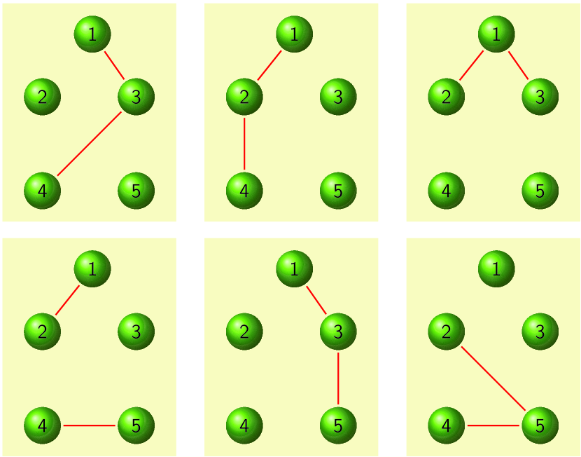
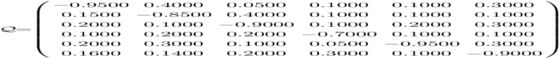
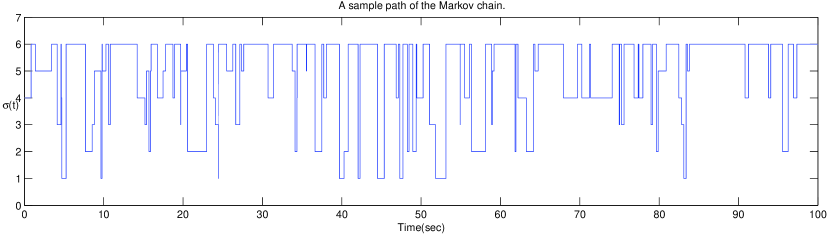
Figure 1: A switching network for the optimization algorithm used in this paper: six possible graphs among which the network switches are shown on the left; the switching Markov chain is given on the right, where the generator is given on the upper right and the Markov Switching is plotted on the bottom right.

For simulation, we chose the noise intensities $\sigma_{ij}=1$, the parameters $\eta_{ij}=1$, the coupling strength $c=2$, and the initial states of five agents as $x_{1}(0)\!=\!(-2,4)^{T}$, $x_{2}(0)\!=\!(-3,3)^{T}$, $x_{3}(0)\!=\!(1,-2)^{T}$, $x_{4}(0)\!=\!(4,2)^{T}$, $x_{5}(0)\!=\!(-3,-4)^{T}$, $\theta_{1}(0)=\cdots=\theta_{5}(0)=1$, $\lambda_{1}(0)\!=\!3$, $\lambda_{2}(0)\!=\!3$, $\nu(0)\!=\!3$. The time evolution of the $x$-states for five agents are illustrated in Figure 2, where the first component of each state $x_{i}$ asymptotically converges to $1$ almost surely (subfigure (a)) and the second component of each state $x_{i}$ asymptotically converges to $2$ almost surely (subfigure (b)). Therefore, each state $x_{i}$ of the 5 agents converges to the optimal solution $(1,2)$ almost surely. Due to space limitation, the time evolutions of the states for $\mbox{\boldmath$\theta$},\mbox{\boldmath$\lambda$},\mbox{\boldmath$\nu$}$ are not plotted here.

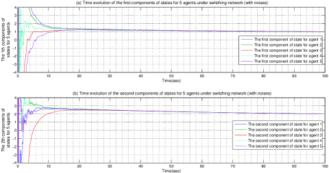
Figure 2: Time evolution of the $x_{i}$ for 5 agents: (a) The first components of $x_{i}^{\prime}s$ converge to $1$; (b) The second components of $x_{i}^{\prime}s$ converge to $2$, both almost surely.

8 Conclusion

This paper has proposed a novel multi-scale method for the distributed convex optimization problem with constraints, and presented in a unified framework to address challenging issues like optimization constraints, communication noises and stochastic networks. Rigorous convergence analysis is given for the proposed algorithm thanks to the use of Lyapunov arguments, Kolmogorov backward equation, and Ito formula. To overcome the technical obstacle in computing the projection in the presence of optimization constraints, we design a projection-free, smooth optimization dynamics for easier analysis and simulation. As a consequence, a major advantage of the proposed multi-scale method presented in this paper is that it generalizes previous distributed convex optimization algorithms from a fixed network topology to the switching case. Also, the stochastic averaging in this paper is a generalization of the deterministic averaging in our earlier works, again thanks to the multi-scale method used in this paper.

Appendix A: Derivation of The SDE (11)

To characterize the noisy term $\omega_{i}:=\sum\nolimits_{j\in\mathscr{N}_{i}(t)}\sigma_{ji}\xi_{ji}(x_{j}-x_{i})$ in equations (10a)-(10b), define $\xi_{i}=[\xi_{1i},\xi_{2i},\cdots,\xi_{Ni}]^{T}$, $i=1,\cdots,N$. Also, for each switching mode $s\in\mathbb{S}$, define $\mathcal{M}^{i}_{s}\!=\![a^{i1}_{s}\sigma_{1i}(x_{1}\!-\!x_{i}),\cdots,a^{iN}_{s}\sigma_{Ni}(x_{N}-x_{i})]$. Then the noisy term $\omega_{i}$ above can be written as $\omega_{i}=\mathcal{M}^{i}_{s}\xi_{i}$. Therefore, the equation (10a) becomes

$$dx_{i}\!=\!\!\left[c\!\sum\nolimits_{\scalebox{0.7}[0.8]{$j\!\in\!\!\mathscr{N}_{i}(t)$}}(x_{j}\!-\!x_{i})\!-\!\theta_{i}\!-\!\nabla f_{i}(x_{i})\!-\!\!\sum\nolimits_{j}^{r_{i}}\!\!\lambda_{ij}\!\nabla g_{ij}(x_{i})\!-\!\sum\nolimits_{j}^{s_{i}}\!\!\nu_{ij}\nabla\!g_{ij}(x_{i})\right]\!dt\!+\!c\mathcal{M}^{i}_{{\sigma(t)}}dw_{i},$$

where $\xi_{i}dt=dw_{i}$ with $w_{i}$ an $N$-dimensional standard Browian motion on the probability space $(\Omega,\mathcal{F},\mathbb{P},\{\mathcal{F}_{t}\}_{t\geq 0})$. Let $\mbox{\boldmath$x$}={\rm col}\{x_{1},\cdots,x_{N}\}$. Define the stacked functions $G(\mbox{\boldmath$x$})={\rm col}\{{\rm col}\{g_{ij}(x_{i})\}_{j=1}^{r_{i}}\}_{i=1}^{N}\in\mathbb{R}^{r}$, $H(\mbox{\boldmath$x$})={\rm col}\{{\rm col}\{h_{ij}(x_{i})\}_{j=1}^{s_{i}}\}_{i=1}^{N}\in\mathbb{R}^{s}$ and the stacked gradients $\nabla F(\mbox{\boldmath$x$})={\rm col}\{\nabla f_{i}(x_{i})\}_{i=1}^{N}\in\mathbb{R}^{nN}$, $\nabla G(\mbox{\boldmath$x$})={\rm col}\big{\{}{\rm col}\{\nabla g_{ij}(x_{i})\}_{j=1}^{r_{i}}\big{\}}_{i=1}^{N}\in\mathbb{R}^{rn}$, $\nabla H(\mbox{\boldmath$x$})={\rm col}\big{\{}{\rm col}\{\nabla h_{ij}(x_{i})\}_{j=1}^{s_{i}}\big{\}}_{i=1}^{N}\in\mathbb{R}^{sn}$. For each switching mode $s\!\in\!\mathbb{S}$, set $\mathcal{M}_{s}\!=\!{\rm diag}\{\mathcal{M}_{s}^{i}\}_{i=1}^{N}$ $\!\in\!\mathbb{R}^{nN\times N^{2}}$. In addition, let $\mbox{\boldmath$w$}\!=\!{\rm col}\{w_{i}\}_{i=1}^{N}\in\mathbb{R}^{N^{2}}$ and define $r\!=\!\sum_{i=1}^{N}r_{i}$, $s\!=\!\sum_{i=1}^{N}s_{i}$. Set $\mbox{\boldmath$\lambda$}\!=\!{\rm col}\{\lambda_{1},\cdots,\lambda_{N}\}\!\in\!\mathbb{R}^{r}$ with $\lambda_{i}\!=\!{\rm col}\{\lambda_{i1},\cdots,\lambda_{ir_{i}}\}\!\in\!\mathbb{R}^{r_{i}}$ , and $\mbox{\boldmath$\nu$}\!=\!{\rm col}\{\nu_{1},\cdots,\nu_{N}\}\!\in\!\mathbb{R}^{s}$ with $\nu_{i}\!=\!{\rm col}\{\nu_{i1},\cdots,\nu_{is_{i}}\}\!\in\!\mathbb{R}^{s_{i}}$ . Define $\mbox{\boldmath$\theta$}={\rm col}\{\theta_{1},\cdots,\theta_{N}\}\in\mathbb{R}^{nN}$. With these, the equation (10) can be written in a compact form as in (11).

Appendix B: Proof of The Inequality (15)

Firstly, for $V_{1}$, defining $\mbox{\boldmath$h$}=\nabla F(\mbox{\boldmath$x$})+\boldsymbol{\lambda}\odot\nabla G(\mbox{\boldmath$x$})+\boldsymbol{\nu}\odot\nabla H(\mbox{\boldmath$x$})$ and $\mbox{\boldmath$h$}^{*}=\nabla F(\mbox{\boldmath$x$}^{*})+\!\boldsymbol{\lambda}^{*}\odot\nabla G(\mbox{\boldmath$x$}^{*})+\boldsymbol{\nu}^{*}\odot\nabla H(\mbox{\boldmath$x$}^{*})$ and noting $\mbox{\boldmath$\theta$}^{*}=-\mbox{\boldmath$h$}^{*}$ in view of (12), the action of the infinitesimal operator $\mathcal{A}$ on $V_{1}$ can be calculated as

$$\mathcal{A}V_{1} =\underbrace{(\mbox{\boldmath$x$}\!-\!\mbox{\boldmath$x$}^{*})^{T}[-c\boldsymbol{\mathcal{L}}\mbox{\boldmath$x$}-\mbox{\boldmath$\theta$}-\nabla F(\mbox{\boldmath$x$})]+\frac{1}{2}c^{2}tr(\mathcal{M}^{T}\mathcal{M})}_{A}-\sum_{i=1}^{N}\sum_{j=1}^{r_{i}}\lambda_{ij}(x_{i}\!-\!x^{*})^{T}\nabla g_{ij}(x_{i})$$

$$\hskip 14.22636pt+\!\underbrace{[(\mbox{\boldmath$x$}\!-\!\mbox{\boldmath$x$}^{*})\!+\!(\mbox{\boldmath$\theta$}\!-\!\mbox{\boldmath$\theta$}^{*})]^{T}[-(\mbox{\boldmath$\theta$}\!-\!\mbox{\boldmath$\theta$}^{*})\!-\!(\mbox{\boldmath$h$}\!-\!\mbox{\boldmath$h$}^{*})]}_{B}-\!\sum_{i=1}^{N}\!\sum_{j=1}^{s_{i}}\!\nu_{ij}(x_{i}-x^{*})^{T}\nabla h_{ij}(x_{i})$$ (27)

The trace ${\rm tr}(\mathcal{M}^{T}\mathcal{M})$ brings difficulty to the convergence analysis. To get rid of this difficulty, we give an estimation of ${\rm tr}(\mathcal{M}^{T}\mathcal{M})$ as follows,

$${\rm tr}(\mathcal{M}^{T}\!\mathcal{M}) =\sum\nolimits_{i=1}^{N}{\rm tr}[(\mathcal{M}^{i})^{T}\mathcal{M}^{i}]=\sum\nolimits_{i=1}^{N}\sum\nolimits_{j=1}^{N}(a^{ij})^{2}(\sigma_{ji})^{2}(x_{j}-x_{i})^{T}(x_{j}-x_{i})$$

$$\leq\kappa^{2}\sum\nolimits_{i=1}^{N}\sum\nolimits_{j=1}^{N}a^{ij}(x_{j}-x_{i})^{T}(x_{j}-x_{i})\!=\!\kappa^{2}\mbox{\boldmath$x$}^{T}\!\boldsymbol{\mathcal{L}}\mbox{\boldmath$x$}.$$ (28)

As for Part A in (Appendix B: Proof of The Inequality (15)) , noting $\mbox{\boldmath$x$}^{T}\!\boldsymbol{\mathcal{L}}\mbox{\boldmath$x$}\!=\!(\mbox{\boldmath$x$}\!-\!\mbox{\boldmath$x$}^{*})^{T}\boldsymbol{\mathcal{L}}(\mbox{\boldmath$x$}\!-\!\mbox{\boldmath$x$}^{*})$ and $\hbar\!=\!\scalebox{1.0}[0.9]{$\frac{1}{2}$}(c\!-\!\frac{1}{2}c^{2}\kappa^{2})$ (c.f. Eq. (14)), the part A can be estimated as $A\!\leq\!(\mbox{\boldmath$x$}\!-\!\mbox{\boldmath$x$}^{*})^{T}\![-\hbar\boldsymbol{\mathcal{L}}\mbox{\boldmath$x$}\!-\!\mbox{\boldmath$\theta$}\!-\!\nabla F(\mbox{\boldmath$x$})]-\hbar(\mbox{\boldmath$x$}\!-\!\mbox{\boldmath$x$}^{*})^{T}\boldsymbol{\mathcal{L}}(\mbox{\boldmath$x$}\!-\!\mbox{\boldmath$x$}^{*})$. Noting that the square bracket is exactly the minus gradient of $\Psi(\mbox{\boldmath$x$},\mbox{\boldmath$\theta$})$ (c.f. Eq. (14)) with respect to $x$ and denoting by $\lambda^{\mathcal{G}}_{2}$ the smallest nonzero eigenvalue of the Laplacian $\mathcal{L}$, one obtains $A\!\leq\!(\mbox{\boldmath$x$}^{*}\!-\!\mbox{\boldmath$x$})^{T}\nabla_{\!\mbox{\boldmath$x$}}\Psi(\mbox{\boldmath$x$},\mbox{\boldmath$\theta$})\!-\!\hbar\lambda^{\mathcal{G}}_{2}(\mbox{\boldmath$x$}\!-\!\mbox{\boldmath$x$}^{*})^{T}(\mbox{\boldmath$x$}\!-\!\mbox{\boldmath$x$}^{*})\!\leq\!\Psi(\mbox{\boldmath$x$}^{*},\mbox{\boldmath$\theta$})\!-\!\Psi(\mbox{\boldmath$x$},\mbox{\boldmath$\theta$})\!-\!\hbar\lambda^{\mathcal{G}}_{2}(\mbox{\boldmath$x$}\!-\!\mbox{\boldmath$x$}^{*})^{T}(\mbox{\boldmath$x$}\!-\!\mbox{\boldmath$x$}^{*})$, where the last inequality uses the fact that $\Psi(\mbox{\boldmath$x$},\mbox{\boldmath$\theta$})$ is convex in its first argument. As for part B in (Appendix B: Proof of The Inequality (15)) , we can prove the inequality $B\leq(\mbox{\boldmath$x$}-\mbox{\boldmath$x$}^{*})^{T}(\mbox{\boldmath$\theta$}-\mbox{\boldmath$\theta$}^{*})+(\mbox{\boldmath$x$}-\mbox{\boldmath$x$}^{*})^{T}(\mbox{\boldmath$x$}-\mbox{\boldmath$x$}^{*})$ by rewriting it into a quadratic form in terms of $\mbox{\boldmath$x$}-\mbox{\boldmath$x$}^{*},\mbox{\boldmath$\theta$}-\mbox{\boldmath$\theta$}^{*},\mbox{\boldmath$h$}-\mbox{\boldmath$h$}^{*}$ and by showing the corresponding matrix to be semi-positive definite. In view of $(\mbox{\boldmath$x$}-\mbox{\boldmath$x$}^{*})^{T}(\mbox{\boldmath$\theta$}-\mbox{\boldmath$\theta$}^{*})=\Psi(\mbox{\boldmath$x$},\mbox{\boldmath$\theta$})-\Psi(\mbox{\boldmath$x$},\mbox{\boldmath$\theta$}^{*})$, one obtains $A+B\leq\left[\Psi(\mbox{\boldmath$x$}^{*},\mbox{\boldmath$\theta$})-\Psi(\mbox{\boldmath$x$},\mbox{\boldmath$\theta$}^{*})\right]-(\hbar\lambda^{\mathcal{G}}_{2}-1)(\mbox{\boldmath$x$}-\mbox{\boldmath$x$}^{*})^{T}(\mbox{\boldmath$x$}-\mbox{\boldmath$x$}^{*})$. Now, $\mathcal{A}V_{1}$ can be calculated as

$$\mathcal{A}V_{1} \leq\Psi(\mbox{\boldmath$x$}^{*},\mbox{\boldmath$\theta$})-\Psi(\mbox{\boldmath$x$},\mbox{\boldmath$\theta$}^{*})\!-\!(\hbar\lambda^{\mathcal{G}}_{2}-1)(\mbox{\boldmath$x$}\!-\!\mbox{\boldmath$x$}^{*})^{T}(\mbox{\boldmath$x$}\!-\!\mbox{\boldmath$x$}^{*})+\!\sum\nolimits_{i=1}^{N}\sum\nolimits_{j=1}^{r_{i}}\lambda_{ij}g_{ij}(x^{*})$$

$$\!-\!\sum\nolimits_{i=1}^{N}\sum\nolimits_{j=1}^{r_{i}}\lambda_{ij}g_{ij}(x_{i})+\sum\nolimits_{i=1}^{N}\sum\nolimits_{j=1}^{s_{i}}\nu_{ij}h_{ij}(x^{*})\!-\!\sum\nolimits_{i=1}^{N}\sum\nolimits_{j=1}^{s_{i}}\nu_{ij}h_{ij}(x_{i}),$$

where we use the convexity of the functions $g_{ij}$ and $h_{ij}$.

Secondly, we calculate the action of the infinitesimal operator $\mathcal{A}$ on $V_{2}+V_{3}$. Firstly note that the function $V_{3}$ can be calculated by the definition of Bregman divergence (c.f. bregman1967 ) as $V_{3}=\sum\nolimits_{i=1}^{N}\sum\nolimits_{j=1}^{r_{i}}(\lambda_{ij}-\lambda_{ij}^{*})-\sum_{(i,j)\in\Omega}\lambda_{ij}^{*}(\ln\lambda_{ij}-\ln\lambda_{ij}^{*})$. Therefore,

$$\mathcal{A}V_{2}+\mathcal{A}V_{3} =\sum\nolimits_{i=1}^{N}\sum\nolimits_{j=1}^{r_{i}}\frac{\eta_{ij}\lambda_{ij}(\lambda_{ij}-\lambda_{ij}^{*})}{1+\eta_{ij}\lambda_{ij}}g_{ij}(x_{i})+\sum\nolimits_{i=1}^{N}\sum\nolimits_{j=1}^{r_{i}}\frac{\lambda_{ij}}{1+\eta_{ij}\lambda_{ij}}g_{ij}(x_{i})$$

$$\hskip 42.67912pt-\sum\nolimits_{(i,j)\in\Omega}\frac{\lambda_{ij}^{*}}{1+\eta_{ij}\lambda_{ij}}g_{ij}(x_{i})=\sum\nolimits_{i=1}^{N}\sum\nolimits_{j=1}^{r_{i}}(\lambda_{ij}-\lambda_{ij}^{*})g_{ij}(x_{i}).$$

Furthermore, the action of the infinitesimal operator $\mathcal{A}$ on $V_{4}$ can be easily calculated as $\mathcal{A}V_{4}=\sum\nolimits_{i=1}^{N}\sum\nolimits_{j=1}^{s_{i}}(v_{ij}-v_{ij}^{*})h_{ij}(x_{i})$. Collecting above results for $\mathcal{A}V_{i},i=1,2,3,4$ and recalling the definition of $\Phi$ in (13), one obtains the inequality (15).

Appendix C: Proof of The Saddle Point Conditions (16)

Due to convexity and affinity, the following results hold

$$\Sigma_{i=1}^{N}f_{i}(x_{i})+\hbar\mbox{\boldmath$x$}\mbox{\boldmath$\mathcal{L}$}\mbox{\boldmath$x$}\geq\Sigma_{i=1}^{N}f_{i}(x^{*})+\Sigma_{i=1}^{N}\nabla f_{i}(x^{*})(x_{i}-x^{*}),$$

$$g_{ij}(x_{i})\geq g_{ij}(x^{*})+\nabla g_{ij}(x^{*})(x_{i}-x^{*}),$$

$$h_{ij}(x_{i})=h_{ij}(x^{*})+\nabla h_{ij}(x^{*})(x_{i}-x^{*}),$$

$$\mbox{\boldmath$x$}-\mbox{\boldmath$x$}^{*}=\mbox{\boldmath$x$}-\mbox{\boldmath$x$}^{*}.$$

Multiplying them by $1,\lambda_{ij}^{*},\nu_{ij}^{*},\mbox{\boldmath$\theta$}^{*}$ respectively (for the forth equality we use $(\mbox{\boldmath$x$}-\mbox{\boldmath$x$}^{*})^{T}\mbox{\boldmath$\theta$}^{*}$ for multiplication) and adding gives $\Phi(\mbox{\boldmath$x$},\mbox{\boldmath$\theta$}^{*},\mbox{\boldmath$\lambda$}^{*},\mbox{\boldmath$\nu$}^{*})\!\geq\!\Phi(\mbox{\boldmath$x$}^{*},\mbox{\boldmath$\theta$}^{*},\mbox{\boldmath$\lambda$}^{*},\mbox{\boldmath$\nu$}^{*})\!+\![\mbox{\boldmath$\theta$}^{*}\!+\!\nabla F(\mbox{\boldmath$x$}^{*})\!+\!\boldsymbol{\lambda}^{*}\!\odot\!\nabla G(\mbox{\boldmath$x$}^{*})\!+\!\boldsymbol{\nu}^{*}\!\odot\!\nabla H(\mbox{\boldmath$x$}^{*})]^{T}(\mbox{\boldmath$x$}\!-\!\mbox{\boldmath$x$}^{*})$. In view of the equation (12), the terms in the square bracket sum to be zero. Therefore, $\Phi(\mbox{\boldmath$x$},\mbox{\boldmath$\theta$}^{*},\mbox{\boldmath$\lambda$}^{*},\mbox{\boldmath$\nu$}^{*})\geq\Phi(\mbox{\boldmath$x$}^{*},\mbox{\boldmath$\theta$}^{*},\mbox{\boldmath$\lambda$}^{*},\mbox{\boldmath$\nu$}^{*})$.

On other hand, noting that ${\color[rgb]{1,0,0}\lambda_{ij}g_{ij}(x_{i}^{*})\leq 0}=\lambda_{ij}^{*}g_{ij}(x_{i}^{*})$ and $h_{ij}(x^{*})=0$, it can be directly checked that $\Phi(\mbox{\boldmath$x$}^{*},\mbox{\boldmath$\theta$},\mbox{\boldmath$\lambda$},\mbox{\boldmath$\nu$})\leq\Phi(\mbox{\boldmath$x$}^{*},\mbox{\boldmath$\theta$}^{*},\mbox{\boldmath$\lambda$}^{*},\mbox{\boldmath$\nu$}^{*})$. This inequality, together with the inequality derived in last paragraph, gives rise to the saddle point condition (16).

Appendix D: Proof of “$\mathcal{A}V=0\Rightarrow(\mbox{\boldmath$x$},\mbox{\boldmath$\theta$},\mbox{\boldmath$\lambda$},\mbox{\boldmath$\nu$})=(\mbox{\boldmath$x$}^{*},\mbox{\boldmath$\theta$}^{*},\mbox{\boldmath$\lambda$}^{*},\mbox{\boldmath$\nu$}^{*})$”

Letting $\mathcal{A}V=0$ gives $(\mbox{\boldmath$x$}-\mbox{\boldmath$x$}^{*})^{T}\,(\mbox{\boldmath$x$}-\mbox{\boldmath$x$}^{*})=0$ and $\Phi(\mbox{\boldmath$x$}^{*},\mbox{\boldmath$\theta$},\mbox{\boldmath$\lambda$},\mbox{\boldmath$\nu$})=\Phi(\mbox{\boldmath$x$},\mbox{\boldmath$\theta$}^{*},\mbox{\boldmath$\lambda$}^{*},\mbox{\boldmath$\nu$}^{*})$, where the former implies $\mbox{\boldmath$x$}=\mbox{\boldmath$x$}^{*}$ and the latter, together with the fact that $(\mbox{\boldmath$x$}^{*},\mbox{\boldmath$\theta$}^{*},\mbox{\boldmath$\lambda$}^{*},\mbox{\boldmath$\nu$}^{*})$ is a saddle point of the Lagrangian $\Phi$, implies $\Phi(\mbox{\boldmath$x$}^{*},\mbox{\boldmath$\theta$},\mbox{\boldmath$\lambda$},\mbox{\boldmath$\nu$})\!=\!\Phi(\mbox{\boldmath$x$},\mbox{\boldmath$\theta$}^{*},\mbox{\boldmath$\lambda$}^{*},\mbox{\boldmath$\nu$}^{*})\!=\!\Phi(\mbox{\boldmath$x$}^{*},\mbox{\boldmath$\theta$}^{*},\mbox{\boldmath$\lambda$}^{*},\mbox{\boldmath$\nu$}^{*})$. Recall that $\mbox{\boldmath$x$}^{*}=\mathbf{1}_{N}\otimes x^{*}$ with $x^{*}$ being the optimal solution which satisfies $g_{ij}(x^{*})\leq 0$ in the KKT condition (5a). Inserting $x_{i}=x^{*}$ into (10c) yields $\dot{\lambda}_{ij}=\frac{\lambda_{ij}g_{ij}(x^{*})}{1+\eta_{ij}\lambda_{ij}}$. If $g_{ij}(x^{*})=0$, then $\dot{\lambda}_{ij}=0$ which implies that $\lambda_{ij}(t)$ stays positive for all $t\geq 0$ since the initial value of $\lambda_{ij}$ is chosen to be positive. If $g_{ij}(x^{*})<0$, then with $g_{ij}(x^{*})=-a<0$, one has $\dot{\lambda}_{ij}=\frac{-a\lambda_{ij}}{1+\eta_{ij}\lambda_{ij}}$ whose trajectory can be shown by elementary analysis as $\lambda_{ij}(t)\geq 0$ for $t\geq 0$ since the initial value of $\lambda_{ij}$ is chosen to be positive. In short, in both cases, for the equation (10c) with $x_{i}=x^{*}$, one has that $\lambda_{ij}(t)\geq 0,\forall t\geq 0$ provided the initial value is positive, and consequently $\dot{\lambda}_{ij}(t)\leq 0$ since $g_{ij}(x^{*})\leq 0$. Therefore, $\lambda_{ij}\geq\lambda_{ij}^{*}$. On the other hand, the fact $\Phi(\mbox{\boldmath$x$}^{*},\mbox{\boldmath$\theta$},\mbox{\boldmath$\lambda$},\mbox{\boldmath$\nu$})\!=\!\Phi(\mbox{\boldmath$x$}^{*},\mbox{\boldmath$\theta$}^{*},\mbox{\boldmath$\lambda$}^{*},\mbox{\boldmath$\nu$}^{*})$ yields $\sum_{i=1}^{N}\sum_{j=1}^{r_{i}}(\lambda_{ij}\!-\!\lambda_{ij}^{*})g_{ij}(x^{*})$ $\!=\!0$. Since $g_{ij}(x^{*})\leq 0$ and $\lambda_{ij}\geq\lambda_{ij}^{*}$, each sum in this summation is non-positive and therefore $(\lambda_{ij}-\lambda_{ij}^{*})g_{ij}(x^{*})=0$, i.e., $\lambda_{ij}g_{ij}(x^{*})=\lambda_{ij}^{*}g_{ij}(x^{*})=0$. This fact implies that the right hand side of equation (10c) with $x_{i}=x^{*}$ is zero and thus $\lambda_{ij}=\lambda_{ij}^{{\dagger}}$ for some constant $\lambda_{ij}^{{\dagger}}\!\geq\!0$. Thus $\lambda_{ij}^{{\dagger}}g_{ij}(x^{*})\!=\!0$. Inserting $\mbox{\boldmath$x$}^{*}\!=\!\mathbf{1}_{N}\otimes x^{*}$ into equations (10b) and (10d) gives that $\theta_{i}=\theta_{i}^{{\dagger}}$ and $\nu_{ij}=\nu_{ij}^{{\dagger}}$ for some constants $\theta_{i}^{{\dagger}}$ and $\nu_{ij}^{{\dagger}}$. Inserting $(\mbox{\boldmath$x$}^{*},\theta_{i}^{{\dagger}},\lambda_{ij}^{{\dagger}},\nu_{ij}^{{\dagger}})$ into (10a) gives $\sum_{i=1}^{N}\nabla f_{i}(x^{*})\!+\!\sum_{i=1}^{N}\sum_{j}^{r_{i}}\lambda_{ij}^{{\dagger}}\nabla g_{ij}(x^{*})\!+\!\sum_{i=1}^{N}\sum_{j}^{s_{i}}\nu_{ij}^{{\dagger}}\nabla h_{ij}(x^{*})\!=\!0$. In conclusion, the KKT conditions (5) are satisfied at the point $(\mbox{\boldmath$x$}^{*},\mbox{\boldmath$\lambda$}^{\dagger},\mbox{\boldmath$\nu$}^{\dagger})$. Then by uniqueness of multipliers in (9), $\lambda_{ij}^{{\dagger}}=\lambda_{ij}^{*}$, $\nu_{ij}^{{\dagger}}=\nu_{ij}^{*}$.

Also, by differentiating both sides of $\Phi(\mbox{\boldmath$x$},\mbox{\boldmath$\theta$}^{*},\mbox{\boldmath$\lambda$}^{*},\mbox{\boldmath$\nu$}^{*})\!=\!\Phi(\mbox{\boldmath$x$}^{*},\mbox{\boldmath$\theta$}^{*},\mbox{\boldmath$\lambda$}^{*},\mbox{\boldmath$\nu$}^{*})$ with respect to $x$ and then by enforcing $\mbox{\boldmath$x$}=\mbox{\boldmath$x$}^{*}$, one obtains $\mbox{\boldmath$\theta$}\!+\!\nabla F(\mbox{\boldmath$x$}^{*})\!+\!\boldsymbol{\lambda}^{*}\!\odot\!\nabla G(\mbox{\boldmath$x$}^{*})\!+\!\boldsymbol{\nu}^{*}\!\odot\!\nabla H(\mbox{\boldmath$x$}^{*})=0$. This, combined with equation (12), gives $\mbox{\boldmath$\theta$}=\mbox{\boldmath$\theta$}^{*}$. In conclusion, letting $\mathcal{A}V=0$ gives rise to $(\mbox{\boldmath$x$},\mbox{\boldmath$\theta$},\mbox{\boldmath$\lambda$},\mbox{\boldmath$\nu$})=(\mbox{\boldmath$x$}^{*},\mbox{\boldmath$\theta$}^{*},\mbox{\boldmath$\lambda$}^{*},\mbox{\boldmath$\nu$}^{*})$.

References

• (1) Nedic, A., Ozdaglar, A.: Distributed subgradient methods for multi-agent optimization. IEEE Transactions on Automatic Control 54(1), 48–61 (2009)
• (2) Nedic, A., Ozdaglar, A., Parrilo, P.A.: Constrained consensus and optimization in multi-agent networks. IEEE Transactions on Automatic Control 55(4), 922–938 (2010)
• (3) Nedic, A., Ozdaglar, A.: Distributed optimization over time-varying directed graphs. IEEE Transactions on Automatic Control 60(3), 615 (2015)
• (4) Boyd, S., Parikh, N., Chu, E., Peleato, B., Eckstein, J.: Distributed optimization and statistical learning via alternating direction method of multipliers. Foundations and Trends in Machine Learning 3(1), 1–122 (2011)
• (5) Feijer, D., Paganini, F.: Stability of primal-dual gradient dynamics and applications to network optimization. Automatica 46(12), 1974–1981 (2010)
• (6) Duchi, J.C., Agarwal, A., Wainwright, M.M.: Dual averaging for distributed optimization: convergence analysis and network scaling. IEEE Transactions on Automatic Control 57(3), 592–606 (2012)
• (7) Ram, S.S., Nedic, A., Veeravalli, V.V.: Distributed stochastic subgradient projection algorithms for convex optimization. Journal of Optimization Theory and Appllications 147, 516–545 (2010)
• (8) Tsitsiklis, J.N., Bertsekas, D.P., Athans, M.: Distributed asynchronous deterministic and stochastic gradient optimization algorithms. IEEE Transactions on Automatic Control 31(9), 803–812 (1986)
• (9) Ram, S.S., Nedic, A., Veeravalli, V.V.: Incremental stochastic subgradient algorithms for convex optimization. Journal of Optimization 20(2), 691–717 (2010)
• (10) Parikh, N.: Proximal algorithms. Foundations and Trends in Optimization 1(3), 123–231 (2013)
• (11) Jakovetic, D., Xavier, J., Moura, J.M.F.: Fast distributed gradient methods. IEEE Transactions on Automatic Control 59(5), 1131–1146 (2014)
• (12) Qu, G., Li, N.: Harnessing smoothness to accelerate distributed optimization. to appear in IEEE Transactions on Control of Network Systems (2017)
• (13) Zeng, X., Yi, P., Hong, Y.: Distributed continuous-time algorithm for constrained convex optimizations via nonsmooth analysis approach. IEEE Transactions on Automatic Control 62(10), 5227–5233 (2017)
• (14) Xin, R., Khan, U.A.: A linear algorithm for optimization over directed graphs with geometric convergence. IEEE Control Systems Letters 2(3) (2018)
• (15) Yuan, D., Ho, D.W.C., Hong, Y.: On convergence rate of distributed stochastic gradient algorithm for convex optimization with inequality constraints. SIAM J. Control and Optimization 54, 2872–2892 (2016)
• (16) Lou, Y., Hong, Y., Wang, S.: Distributed continuous-time approximate projection protocols for shortest distance optimization problems. Automatica 69, 289–297 (2016)
• (17) Charalamous, C.: Distributed constrained optimization by consensus-based primal-dual perturbation method. IEEE Transactions on Automatical Control 59(6) (2014)
• (18) Yi, P., Hong, Y., Liu, F.: Distributed gradient algorithm for constrained optimization with application to load sharing in power systems. Systems and Control Letters 83, 45–52 (2015)
• (19) Zhu, M., Mart nez, S.: On distributed convex optimization under inequality and equality constraints. IEEE Transactions on Automatic Control 57(1), 691–719 (2011)
• (20) Yamashita, S., Hatanaka, T., Yamauchi, J., Fujita, M.: Passivity-based generalization of primal-dual dynamics for non-strictly convex cost functions. Automatica 112, 108,712 (2020)
• (21) Nemirovsky, A.S., Yudin, D.B.: Problem Complexity and Method Efficiency in Optimization. John Wiley and Sons, Chichester (1983)
• (22) Raginsky, M., Bouvrie, J.: Continuous-time stochastic mirror descent on a network: variance reduction, consensus, convergence. The 51st IEEE Conference on Decision and Control pp. 6793–6800 (2012)
• (23) Xie, P., You, K., Tempo, R., Wu, C.: Distributed convex optimization with inequality constraints over time-varying unbalanced digraphs. to appear in IEEE Transactions on Automatic Control (2018)
• (24) Lobel, I., Ozdaglar, A.: Distributed subgradient methods for convex optimization over random networks. IEEE Transactions on Automatical Control 56(6), 1291–1306 (2011)
• (25) Ni, W., Wang, X.: Averaging method to distributed convex optimization for continuous-time multi-agent systems. Kybernetika 52(6), 898–913 (2016)
• (26) Ni, W., Wang, X., Xiong, C.: Consensus controllability, observability and robust design for leader-following linear multi-agent systems. Automatica 49(7), 2199–2205 (2013)
• (27) Ni, W., Wang, X., Xiong, C.: Leader-following consensus of multiple linear systems under switching topologies: an averaging method. Kybernetika 48(6), 1194–1210 (2012)
• (28) Ni, W., Zhao, D., Ni, Y., Wang, X.: Stochastic averaging approach to leader-following consensus of linear multi-agent systems. Journal of the Franklin Institute 353(12), 2650–2669 (2016)
• (29) Haken, H.: Synergetik. New York: Springer-Verlag (1982)
• (30) Pavliotis, G.V., Stuart, A.M.: Multiscale Methods: Averaging and Homogenization. New York: Springer-Verlag (2008)
• (31) Wolfowitz, J.: Products of indecomposable, aperiodic, stochastic matrices. Proceedings of the American Mathematical Sociaty 14(4), 733–737 (1963). DOI: 10.1109/TAC.2016.2628807
• (32) Boyd, S., Vandenberghe, L.: Convex Optimization. Cambridge University Press (2004)
• (33) Wachsmuth, G.: On licq and the uniqueness of lagrange multipliers. Operations Research Letters 41(1), 78–80 (2013)
• (34) Li, T., Wu, F., Zhang, J.: Multi-agent consensus with relative-state-dependent measurement noises. IEEE Transactions on Automatic Control 59(9), 2463–2468 (2014)
• (35) Carli, R., Fagnani, F., Speranzon, A., Zampiei, S.: Communication constraints in the average consensus problem. IEEE Transactions on Automatical Control 44(3) (2008)
• (36) Wang, J., Elia, N.: Mitigation of complex behavior over networked systems: analysis of spatially invariant structures. Automatica 49(6), 1626–1638 (2013)
• (37) Kia, S.S., Cort s, J., Mart nez, S.: Distributed convex optimization via continuous-time coordination algorithms with discrete-time communication. Automatica 55, 254–264 (2015)
• (38) Brunner, F.D., Dürr, H.B., Ebenbauer, C.: Feedback design for multi-agent systems: a saddle point approach. The 51th IEEE Conference on Decision and Control, Hawail, USA pp. 3783–3789 (2012)
• (39) Bregman, L.M.: The relaxation method of finding the common points of convex sets and its application to the solution of problems in convex programming. USSR Computational Mathematics and Mathematical Physics 7(3), 200–217 (1967)
• (40) Mao, X.: Stochastic versions of the lasalle theorem. Journal of Differential Equations 153, 175–195 (1999)
• (41) Freedman, D.: Markov Chains. New York: Springer-Verlag (1983)
• (42) Fragoso, M.D., Costa, O.L.V.: A unified approach for stochastic and mean square stability of continuous-time linear systems with markovian jumping parameters and additive disturbances. SIAM Journal on Control and Optimization 44(4), 1165–1190 (2015)
• (43) Evans, L.C.: Partial Differential Equations (second edition). American Math Society (2010)