A Minimax Probability Machine for
Non-Decomposable Performance Measures

Abstract

Imbalanced classification tasks are widespread in many real-world applications. For such classification tasks, in comparison with the accuracy rate, it is usually much more appropriate to use non-decomposable performance measures such as the Area Under the receiver operating characteristic Curve (AUC) and the $F_{\beta}$ measure as the classification criterion since the label class is imbalanced. On the other hand, the minimax probability machine is a popular method for binary classification problems and aims at learning a linear classifier by maximizing the accuracy rate, which makes it unsuitable to deal with imbalanced classification tasks. The purpose of this paper is to develop a new minimax probability machine for the $F_{\beta}$ measure, called MPMF, which can be used to deal with imbalanced classification tasks. A brief discussion is also given on how to extend the MPMF model for several other non-decomposable performance measures listed in the paper. To solve the MPMF model effectively, we derive its equivalent form which can then be solved by an alternating descent method to learn a linear classifier. Further, the kernel trick is employed to derive a nonlinear MPMF model to learn a nonlinear classifier. Several experiments on real-world benchmark datasets demonstrate the effectiveness of our new model.

1 Introduction

Binary classification may be the most encountered problems in real-world applications and has been extensively studied. The standard binary model seeks to learn a classifier by maximizing the Accuracy Rate (AR) or minimizing the error rate. However, the accuracy rate is not an appropriate metric in the setting where the label class is imbalanced [36, 11, 35, 41]. A simple majority algorithm can guarantee a high prediction accuracy in such a case. Many algorithms were devised to deal with imbalanced classification problems, based on the cost-sensitive learning and resampling techniques [6, 25, 15, 24, 28, 34]. A comprehensive survey on related works can be found in [15, 23, 13]. The classical imbalanced learning algorithms aim at maximizing a modified accuracy rate. Several other evaluation metrics have been proposed to measure the learned classifier, including AUC, $F_{\beta}$-measure, and the geometric mean of the True Positive Rate (TPR) and the True Negative Rate (TNR) [16, 5, 47], which are more appropriate for imbalanced classification tasks. But, different from the accuracy rate, these measures can not be expressed as a sum of independent metrics on individual examples and thus are called non-decomposable performance measures. They give a more holistic evaluation of the entire data, which makes them challenging to be optimized.

In recent years, many methods have been proposed which focus on optimizing non-decomposable performance measures [1, 43, 27, 12, 37]. By [46], these methods fall into two groups: the Empirical Utility Maximization (EUM) and the Decision-Theoretic Approach (DTA).

EUM is also called the Population Utility (PU) in [10]. It learns a classifier by maximizing the corresponding empirical measures based on the training data and then predicts an unseen instance by using the learned classifier. Several works have applied the traditional algorithms, such as SVM and logistic regression, to the non-decomposable performance measure maximization by replacing the error rate with a specially designed surrogate loss function [36, 20, 22, 8]. Recently, studies are focused on the plug-in approach, which learns a class probability function first based on a training example and then makes a decision of the threshold according to another data set [35, 46, 26]. [39] provided a general methodology to show the statistical consistency of the plug-in approach for any performance measure that can be expressed as a continuous function of the true positive and true negative rates as well as the class proportion, such as $F_{\beta}$ and the Geometric Mean (GM) of TPR and TNR. Cost-sensitive classification is also used in this approach, which learns a classifier by minimizing a weighted False Positive Rate (FPR) and False Negative Rate (FNR). [35] proved the consistency of the empirically cost-sensitive learning algorithm concerning the Arithmetic Mean (AM) of the TPR and TNR metrics, in which the cost parameter is determined from the empirical class ratio. A cost-sensitive Support Vector Machine (SVM) with a tuning threshold was proposed in [41] for the metric $F_{\beta}$, where the cost parameter is searched with a grid-based method. [1] presented the Cone-based Optimal Next Evaluation (CONE) algorithm that iteratively selects the classification costs that lead to a near-optimal $F_{\beta}$-measure. As discussed in Section 2, many non-decomposable performance measures except AM aim at minimizing a polynomial combination of FPR and FNR rather than a linear combination of them. The cost-sensitive learning approach seems not an appropriate method for these metrics.

DTA was first proposed in [31]. It considers set classifiers and predicts the label of a test set by maximizing its expected measure. Thus it needs the entire joint distribution of the ground-truth which can be estimated by using the maximum likelihood principle or the logistic regression model. Several methods have been proposed to solve this type of problems, based on the assumption that the labels are independent [31, 21, 46]. Later, in [11, 45] this assumption was removed, and a general algorithm was given which needs only $n^{2}+1$ parameters of the joint distribution, where $n$ is the sample size. The above work focused on the $F_{\beta}$ metric. Recently, a general analysis of DTA was provided in [40] for non-decomposable performance measures. It is also named the Expected Test Utility (ETU) in [10].

The Minimax Probability Machine (MPM) method is a competitive algorithm for binary classification problems which was first proposed in [29]. It aims at maximizing the accuracy rate of a random instance in a worst-case setting, where only the mean and covariance matrix of each class are assumed to be known [29]. It forces the worst-case probability of misclassification of each class to be exactly equal, which is usually not true in real-world applications. The minimum error minimax probability machine (MEMPM) removes this constraint and seeks to learn a linear classifier by minimizing a weighted probability of misclassification of the future data in the same worst-case setting [19]. However, MPM and MEMPM are not suitable for imbalanced classification tasks since they are based on the accuracy rate which is not an appropriate metric for such tasks, as mentioned above.

In this paper, we develop an MPM model based on non-decomposable performance measures for the first time. This model can deal with imbalanced classification tasks where the mean and covariance matrix of data are given or can be estimated, which is different from [29, 19]. We first present a minimax probability machine for the $F_{\beta}$-measures (MPMF) and then briefly discuss how to extend it to several other non-decomposable performance measures as listed in Table 1. Further, to solve MPMF effectively, its equivalent minimization formulation is derived whose objective function is given in terms of a polynomial combination of FPR and FNR. The equivalent minimization problem is then solved by the alternative descent method. The convergence of the method is also analyzed and verified numerically. Furthermore, we explore the kernel trick in the setting to obtain a nonlinear MPM model, yielding a nonlinear classifier which can effectively deal with nonlinearly separable imbalanced problems. Note that, due to the difficulty caused by the non-decomposability, most of the existing works related to non-decomposable metrics only consider linear models. A main feature of our method is that it only makes use of the mean and covariance matrix of data and thus is independent of the training data size, making our method appropriate for large-scale problems. Another feature of our method is that it has no hyper-parameters to choose. Several experiments on real world benchmark datasets presented in the paper and compared with the plug-in method (a state-of-the-art method) illustrate that our MPMF method is effective for imbalanced classification problems.

The paper is organized as follows. In Section 2, we introduce several non-decomposable performance measures for binary classification and derive their equivalent minimization objective functions, which can be expressed as a polynomial combination of FPR and FNR. In Section 3, the minimax probability machine and its variants for the accuracy rate maximization are presented. In Section 4, we present the MPM model with the $F_{\beta}$ metric which is then solved by using the alternative descent method. In Section 5, we propose a non-linear $F_{\beta}$ maximization based on the kernel trick and the minimax probability machine. Several experiments are presented in Section 6, and conclusions are given in Section 7.

Table 1: Non-decomposable Performance Measures: AR, AM, QM, $F_{\beta}$, HM, GM, G-TP/PR, JAC (first column), their definition (second column) and their equivalent minimization objective function given in terms of a polynomial combination of FPR and FNR (third column)

Measure	Definition ($P_{nd}(\mbox{TPR},\mbox{TNR})$)	Minimization Objective ($Q_{nd}(\mbox{FNR},\mbox{FPR})$)
AR	$p\cdot\mbox{TPR}+(1-p)\cdot\mbox{TNR}$	$p\cdot\mbox{FNR}+(1-p)\cdot\mbox{FPR}$
AM	$(\mbox{TPR}+\mbox{TNR})/2$	$(\mbox{FNR}+\mbox{FNR})/2$
QM	$1-[(1-\mbox{TPR})^{2}+(1-\mbox{TNR})^{2}]/2$	$[(\mbox{FNR})^{2}+(\mbox{FPR})^{2}]/2$
$F_{\beta}$	$\frac{(1+\beta^{2})p\cdot\mbox{TPR}}{(1+\beta^{2})p\cdot\mbox{TPR}+(1-p)\cdot\mbox{FPR}+\beta^{2}p\cdot\mbox{FNR}}$	$\sum_{i=0}^{\infty}(\beta^{2}p\cdot\mbox{FNR}+(1-p)\cdot\mbox{FPR})(\mbox{FNR})^{i}$
HM	${2\cdot\mbox{TPR}\cdot\mbox{TNR}}/[{\mbox{TPR}+\mbox{TNR}}]$	$\sum_{i=0}^{\infty}[(\mbox{FNR})^{i}+(\mbox{FPR})^{i}]$
GM	$\sqrt{\mbox{TPR}\cdot\mbox{TNR}}$	$[\sum_{i=0}^{\infty}(\mbox{FPR})^{i}][\sum_{i=0}^{\infty}(\mbox{FNR})^{i}]$
G-TP/PR	$\sqrt{\mbox{TPR}\cdot\mbox{Prescison}}$	$p\sum_{i=0}^{\infty}(\mbox{FNR})^{i}+(1-p)\cdot\mbox{FPR}\sum_{i=0}^{\infty}[\mbox{FNR}\cdot(2-\mbox{FNR})]^{i}$
JAC	${p\cdot\mbox{TPR}}/[{p\cdot\mbox{TPR}+p\cdot\mbox{FNR}+(1-p)\cdot\mbox{FPR}}]$	$[p\cdot\mbox{FNR}+(1-p)\cdot\mbox{FPR}]\sum_{i=0}^{\infty}(\mbox{FNR})^{i}$

2 Problem Setting

In this section, we present several non-decomposable performance measures in binary classification.

2.1 Binary Classification

Let ${\mathcal{X}}\subset{\mathbb{R}}^{d}$ be the instance space and let ${\mathcal{Y}}=\{+1,-1\}$ be the label set with the distribution ${\cal D}$ over ${\mathcal{X}}\times{\mathcal{Y}}$. We aim to learn a classifier $f\in\mathcal{F}$, which predicts a label based on the seeing feature and makes a minimal prediction error rate. Given a classifier $f:{\mathcal{X}}\to{\mathbb{R}}$ and an instance $x\in{\mathcal{X}}$, the label of $x$ is assigned to be $+1$ if $f(x)>0$, and $-1$ if otherwise. Then the binary classification problem can be expressed as

$$\arg_{f\in\mathcal{F}}\max_{(x,y)\sim{\cal D}}{\bf Pr}(yf(x)>0).$$ (1)

Note that the prior knowledge of the instance space plays a key role in machine learning problems. Suppose the true distribution ${\cal D}$ is explicitly given. Then the Bayesian estimator can be computed by solving (1). If the distribution class is given, we can first estimate the distribution ${\cal D}$ with the maximum likelihood method and then learn a classifier. In general, the true distribution ${\cal D}$ or its distribution class is not known in practice. But the moment statistics of the input space can be estimated, and thus the minimax probability machine can be developed. In the worst-case, the sample data can be used to learn a classifier by minimizing the empiric risk.

2.2 Non-decomposable Performance Measures

Let $p={\bf Pr}(y=+1)$ be the probability of the positive examples. We now introduce some basic notations:

TPR $$:= 1-\mbox{FNR}={\bf Pr}(\hat{y}=+1|y=+1),$$

TNR $$:= 1-\mbox{FPR}={\bf Pr}(\hat{y}=-1|y=-1),$$

Precision $$:= {\bf Pr}(y=1|\hat{y}=1)$$

$$= \frac{p\cdot\mbox{TPR}}{p\cdot\mbox{TPR}+(1-p)\cdot\mbox{FPR}}$$

A better classifier should have a greater TPR, TNR, and precision values, but there is a tradeoff among these measures. It is unable to achieve the optimal values simultaneously for TPR, TNR, and precision since each of these quantities can be maximized at the cost of other measures. So usually we consider the criterion that adjusts the basic quantities, such as several combinations of TPR and TNR. Table 1 presents some usually used performance measures. In this paper, we focus on the $F_{\beta}$ measure, which is a harmonic mean of TPR and Precision and defined as

$$F_{\beta} = \frac{(\beta^{2}+1)\cdot\mbox{TPR}\cdot\mbox{Precision}}{\beta^{2}\cdot\mbox{Precision}+\mbox{TPR}}$$

$$= \frac{(1+\beta^{2})\cdot p\cdot\mbox{TPR}}{(1+\beta^{2})\cdot p\cdot\mbox{TPR}+(1-p)\cdot\mbox{FPR}+\beta^{2}p\cdot\mbox{FNR}}$$

A larger $F_{\beta}$ means a better corresponding classifier.

Lemma 1.

The classifier $f$ maximizes $F_{\beta}$ if and only if it minimizes $Q_{F}$, where $Q_{F}$ is a polynomial combination function of FPR and FNR defined by

$$Q_{F} = \sum_{i=0}^{\infty}((1-p)\cdot\mbox{FPR}+\beta^{2}p\cdot\mbox{FNR})\cdot(\mbox{FNR})^{i}$$

$$= \frac{(1-p)\cdot\mbox{FPR}+\beta^{2}p\cdot\mbox{FNR}}{1-\mbox{FNR}}.$$

Proof.

Since $F_{\beta}>0$, then maximizing $F_{\beta}$ is equivalent to minimizing ${1}/{F_{\beta}}$. We have

$$\frac{1}{F_{\beta}} = 1+\frac{(1-p)\cdot\mbox{FPR}+\beta^{2}p\cdot\mbox{FNR}}{p(1+\beta^{2})(1-\mbox{FNR})}$$

$$= 1+\sum_{i=0}^{\infty}\frac{[(1-p)\cdot\mbox{FPR}+\beta^{2}p\cdot\mbox{FNR}]\cdot(\mbox{FNR})^{i}}{p(1+\beta^{2})}$$

The proof is thus complete.

Note that the above method can be extended to other non-decomposable performance measures, such as the AM, the GM, the Quadratic Mean (QM) of TPR and TNR, the Harmonic Mean (HM) of TPR and TNR, the Geometric Mean (GM) of TPR and TNR, the Geometric mean of TPR and PRecision (G-TP/PR), and the Jaccard Coefficient (JAC). Maximizing these measures is also equivalent to minimizing $Q_{nd}$, which can also be expressed as a polynomial combination of FPR and FNR, that is, $Q_{nd}=\sum_{i,j=0}^{\infty}\tau_{ij}(\mbox{FPR})^{i}(\mbox{FNR})^{j}$ (see the third column in Table 1). It is interesting to note that the same minimizing objective function is obtained for both the $F_{1}$ measure and the JAC measure, which was overlooked previously in the literature. Note further that the objective measure is replaced with a well-defined weighted linear combination of FNR and FPR in the cost-sensitive approach, but a polynomial combination of FRP and FNP is minimized in this paper.

3 MPM with the Accuracy Rate Measure

Different from the traditional classification algorithms, such as SVMs and neural networks, which seek to learn a real-valued function by minimizing the error rate on a given training data set, MPM tries to separate the two classes of the data samples with the maximal probability in a worst-case setting where only the mean and covariance matrix of each class are given in advance [29]. Let the notation $x\sim(\mu,\Sigma)$ denote that $x$ belongs to the class of distributions having the mean $\mu$ and the covariance matrix $\Sigma$. Assume that the mean and covariance matrix of the positive and negative samples, denoted, respectively, by $\{\mu_{P},\Sigma_{P}\}$ and $\{\mu_{N},\Sigma_{N}\}$, are all reliable. Then MPM can be expressed as the optimization problem

$$\begin{split}&\max_{0<\alpha<1,w\neq 0,b}\alpha\qquad\\ \text{s.t.}&\inf_{x_{P}\sim(\mu_{P},\Sigma_{P})}{\rm\bf Pr}\{w^{T}x_{P}\geq b\}\geq\alpha\\ &\inf_{x_{N}\sim(\mu_{N},\Sigma_{N})}{\rm\bf Pr}\{w^{T}x_{N}\leq b\}\geq\alpha\end{split}$$ (2)

where the inf is taking over all distributions with mean $\mu$ and covariance matrix $\Sigma$. Let $(\alpha^{\star},w^{\star},b^{\star})$ be the optimal solution of (2). It is guaranteed that the misclassification probability is less than $1-\alpha^{\star}$ for any future data sample with the learned classifier $f(x)=(w^{\star})^{T}x-b^{\star}$.

To solve the optimization problem (2), we need to remove the unknown probability in the constraint by using the following result established in [33] (see also Theorem 6.1 in [2]).

Lemma 2.

Suppose $x\in{\mathbb{R}}^{p}$ is a random vector with $x\sim(\mu,\Sigma)$ and $S\subset{\mathbb{R}}^{p}$ is a given convex set. Then the supremum of the probability of $x\in S$ is given as $\sup_{x\sim(\mu,\Sigma)}{\rm\bf Pr}(x\in S)={1}/({1+d^{2}})$, where $d^{2}=\inf_{x\in S}(x-\mu)^{T}\Sigma^{-1}(x-\mu)$.

If the convex set $S$ is a half-space, then $d$ can be calculated explicitly, leading to the following lemma which was proved in [29].

Lemma 3.

Given $w\in{\mathbb{R}}^{p}$ with $p\neq 0$ and $b\in{\mathbb{R}}$, the condition

$$\inf_{x\sim(\mu,\Sigma)}{\rm\bf Pr}\{w^{T}x\leq b\}\geq\alpha$$

holds if and only if

$$b-w^{T}x\geq\kappa(\alpha)\sqrt{w^{T}\Sigma w},$$

where $\kappa(\alpha)=\sqrt{{\alpha}/({1-\alpha})}$.

It is easy to see that $\kappa(\alpha)$ is a monotonically increasing function of $\alpha$. By Lemma 3, the MPM problem (2) becomes

$$\max_{0<\alpha<1,w\neq 0,b}\kappa(\alpha)\qquad$$

s.t. $$-b+w^{T}\mu_{P}\geq\kappa(\alpha)\sqrt{w^{T}\Sigma_{P}w}$$

$$b-w^{T}\mu_{N}\geq\kappa(\alpha)\sqrt{w^{T}\Sigma_{N}w}.$$

Further, by eliminating $b$ the above problem reduces to

$$\max_{\gamma,w\neq 0}\gamma,$$

s.t. $$w^{T}(\mu_{P}-\mu_{N})\geq\gamma\left[\sqrt{w^{T}\Sigma_{P}w}+\sqrt{w^{T}\Sigma_{N}w}\right]$$

Without loss of generality, we may set $w^{T}(\mu_{P}-\mu_{N})=1$ (see [29]). As a result, MPM is finally equivalent to the following constrained second-order cone programming (SOCP):

$$\min_{w\neq 0}\|\Sigma_{P}^{1/2}w\|_{2}+\|\Sigma_{N}^{1/2}w\|_{2}$$

s.t. $$w^{T}(\mu_{P}-\mu_{N})=1$$

The above SOCP problem can be solved by the interior point method [3]. Now, write $w=w_{0}+Fu$ with $w_{0}=({\mu_{P}-\mu_{N}}){\|\mu_{P}-\mu_{N}\|_{2}^{-2}}$ and $F\in{\mathbb{R}}^{p\times(p-1)}$ the orthogonal matrix whose columns span the subspace of the vectors orthogonal to $(\mu_{P}-\mu_{N})$. Then the constraint can be eliminated to get the unconstrained SOCP [29]:

$$\min_{u\neq 0}\|\Sigma_{P}^{1/2}(w_{0}+Fu)\|_{2}+\|\Sigma_{N}^{1/2}(w_{0}+Fu)\|_{2},$$

A block coordinate descent method is then used to solve the above equivalent unconstrained SOCP [29].

In many real-world applications, the tolerance of the misclassification probability may be different for the positive and negative classes, as seen in the disease diagnosis problem. Thus it is worth increasing the TPR measure at the expense of a lower TNR measure, leading to the biased minimax probability machine (BMPM) and the minimum error minimax probability machine (MEMPM) [19, 18]. MEMPM can be expressed as

$$\begin{split}&\max_{0<\alpha_{1}<1,0<\alpha_{2}<1,w\neq 0,b}p\alpha_{1}+(1-p)\alpha_{2}\qquad\\ \text{s.t.}&\inf_{x_{P}\sim(\mu_{P},\Sigma_{P})}{\rm\bf Pr}\{w^{T}x_{P}\geq b\}\geq\alpha_{1}\\ &\inf_{x_{N}\sim(\mu_{N},\Sigma_{N})}{\rm\bf Pr}\{w^{T}x_{N}\leq b\}\geq\alpha_{2}.\end{split}$$ (3)

If $\alpha_{2}\in(0,1)$ is a predefined constant, then (3) becomes the BMPM problem. The objective function in (3) is a weighted misclassification probability. Lemma 3 can also be applied to simplify the optimization problem (3). Let $(\alpha_{1}^{\star},\alpha_{2}^{\star},w^{\star},b^{\star})$ be the optimal solution of (3) and let $f(x)={w^{\star}}^{T}x-b^{\star}$ be the learned classifier. Then it is guaranteed that the obtained TPR and TNR are at least equal to $\alpha_{1}^{\star}$ and $\alpha_{2}^{\star}$, respectively. In MEMPM, $\alpha_{1}^{\star}$ and $\alpha_{2}^{\star}$ are not necessarily the same, which is different from the case in MPM. Further, the experimental results obtained in [19] demonstrate the effectiveness of MEMPM. Setting $p=1/2$ in the optimization problem (3), a biased minimax probability machine was derived in [17] for imbalanced classification problems. This machine tries to maximize the AM performance measure in a worst-case setting where only the mean and covariance matrix of each class are given. It can be regarded as a special case of our method, as will be illustrated in the next section.

4 MPM with non-decomposable performance measures

In this section, we develop an MPM method with non-decomposable performance measures to deal with imbalanced classification tasks. We first consider the $F_{\beta}$ measure.

For an imbalanced classification problem, suppose the probability of an instance belonging to the positive class $p$ is small enough. Then the MEMPM problem (3) is equivalent to maximizing $\alpha_{2}$ or TNR, which is not appropriate for this case. To address this issue, we replace the objective function in (3) with the global performance metric $F_{\beta}$, which is a function of TPR (or $\alpha_{1}$) and TNR (or $\alpha_{2}$). Thus we get the problem

$$\begin{split}&\max_{0<\alpha_{1}<1,0<\alpha_{2}<1,w\neq 0,b}F_{\beta}\\ \text{s.t.}&\inf_{x_{P}\sim(\mu_{P},\Sigma_{P})}{\rm\bf Pr}\{w^{T}x_{P}\geq b\}\geq\alpha_{1}\\ &\inf_{x_{N}\sim(\mu_{N},\Sigma_{N})}{\rm\bf Pr}\{w^{T}x_{N}\leq b\}\geq\alpha_{2}\end{split}$$ (4)

By Lemma 1, maximizing $F_{\beta}$ is equivalent to minimizing $Q_{F}$. Set $\alpha_{P}=\mbox{FNR}$, $\alpha_{N}=\mbox{FPR}$. Then (4) becomes

$$\begin{split}&\min_{\alpha_{P},\alpha_{N},w\neq 0,b}\frac{(1-p)\alpha_{N}+\beta^{2}p\alpha_{P}}{1-\alpha_{P}}\\ \text{s.t.}&\inf_{x_{P}\sim(\mu_{P},\Sigma_{P})}{\rm\bf Pr}\{w^{T}x_{P}\geq b\}\geq 1-\alpha_{P}\\ &\inf_{x_{N}\sim(\mu_{N},\Sigma_{N})}{\rm\bf Pr}\{w^{T}x_{N}\leq b\}\geq 1-\alpha_{N}\\ &0<\alpha_{P}<1,\;0<\alpha_{N}<1\end{split}$$ (5)

We call this model the minimax probability machine for the $F_{\beta}$-measure (MPMF). For simplicity, define $Q_{F}(\alpha_{P},\alpha_{N};w):=[(1-p)\alpha_{N}+\beta^{2}p\alpha_{P}](1-\alpha_{P})^{-1}$ and omit the conditions $0<\alpha_{P}<1,0<\alpha_{N}<1$ in what follows. Note that these two constrained conditions are guaranteed to be satisfied by the optimal value of $\alpha_{P},\alpha_{N}$ obtained below (see (11) and the sentences following (12) below). Suppose $(\alpha_{P}^{\star},\alpha_{N}^{\star},w^{\star},b^{\star})$ is the optimal solution of the MPMF problem (5) and $f(x)=({w^{\star}})^{T}x-b^{\star}$ is the learned classifier. Then the $F_{\beta}$ metric is bigger than $({(1+\beta^{2})p})[{Q^{\star}+(1+\beta^{2})p}]^{-1}$ for any future data sample, where $Q^{\star}=Q_{F}(\alpha_{P}^{\star},\alpha_{N}^{\star};w^{\star})$.

We now propose an algorithm to solve the optimization problem (5). By Lemma 3, we can remove the probability terms without any distribution assumption and obtain the following optimization problem which is equivalent to the problem (5):

$$\begin{split}&\min_{\alpha_{P},\alpha_{N},w\neq 0,b}\frac{(1-p)\alpha_{N}+\beta^{2}p\alpha_{P}}{1-\alpha_{P}}\qquad\\ \text{s.t.}\;\;\;&w^{T}\mu_{P}-b\geq\pi(\alpha_{P})\sqrt{w^{T}\Sigma_{P}w}\\ &b-w^{T}\mu_{N}\geq\pi(\alpha_{N})\sqrt{w^{T}\Sigma_{N}w}\end{split}$$ (6)

where $\pi(\alpha)={1}/{\kappa(\alpha)}=\sqrt{({1-\alpha})/{\alpha}}$ is monotonically decreasing with $\alpha$.

Lemma 4.

The minimal value of (6) is achieved when the two inequalities in the constraints become equalities.

Proof.

Assume that the optimal solution of (6) is $(w^{\star},b^{\star},\alpha_{P}^{\star},\alpha_{N}^{\star})$ and the two inequalities in the constraints hold strictly, that is,

$$(w^{\star})^{T}\mu_{P}-b^{\star}>\pi(\alpha_{P}^{\star})\sqrt{(w^{\star})^{T}\Sigma_{P}w^{\star}},$$

$$b^{\star}-(w^{\star})^{T}\mu_{N}>\pi(\alpha_{N}^{\star})\sqrt{(w^{\star})^{T}\Sigma_{N}w^{\star}}.$$

Then the objective value is getting smaller with $\alpha_{P}^{\star}$ and $\alpha_{N}^{\star}$ decreasing while the constraints remain to hold. This is a contradiction to the fact that $(w^{\star},b^{\star},\alpha_{P}^{\star},\alpha_{N}^{\star})$ is the optimal solution of (6). The proof is thus complete.

By Lemma 4, (6) can be rewritten as:

$$\begin{split}&\min_{\alpha_{P},\alpha_{N},w\neq 0,b}\frac{(1-p)\alpha_{N}+\beta^{2}p\alpha_{P}}{1-\alpha_{P}}\qquad\\ \text{s.t.}\;\;\;&w^{T}\mu_{P}-b=\pi(\alpha_{P})\sqrt{w^{T}\Sigma_{P}w}\\ &b-w^{T}\mu_{N}=\pi(\alpha_{N})\sqrt{w^{T}\Sigma_{N}w}\end{split}$$ (7)

By eliminating $b$ from (7), the two equality constraints become

$$\pi(\alpha_{N})\sqrt{w^{T}\Sigma_{N}w}+\pi(\alpha_{P})\sqrt{w^{T}\Sigma_{P}w}=w^{T}\mu_{pn},$$ (8)

where $\mu_{pn}=\mu_{P}-\mu_{N}$. Note that (8) is positively homogeneous in $w$. Therefore we need to give an additional constraint on $w$. Following [29] and [19] we may set $w^{T}(\mu_{P}-\mu_{N})=1$ without loss of generality, leading to the constrained SOCP subproblem. Following [9], we set $\|w\|=1$, leading to a constrained concave (or convex) optimization problem which is easier to solve (see (14) below). The problem (7) is then transformed into the problem

$$\begin{split}&\min_{\alpha_{P},\alpha_{N},w}\frac{(1-p)\alpha_{N}+\beta^{2}p\alpha_{P}}{1-\alpha_{P}}\\ \text{s.t.}\;\;&\|w\|=1\\ &\pi(\alpha_{N})\sqrt{w^{T}\Sigma_{N}w}+\pi(\alpha_{P})\sqrt{w^{T}\Sigma_{P}w}=w^{T}\mu_{pn}\end{split}$$ (9)

We apply the alternative descent method to solve the non-convex problem (9). Details are presented in Algorithm 1. We initialize the classifier $w_{1}=({\mu_{P}-\mu_{N}})/{\|\mu_{P}-\mu_{N}\|}$, so $\|w_{1}\|=1$. Assume that at the $t$-th round, we have obtained the classifier $w_{t}$ with $\|w_{t}\|=1.$ Let $A_{t}=\sqrt{w_{t}^{T}\Sigma_{P}w_{t}}$, $B_{t}=\sqrt{w_{t}^{T}\Sigma_{N}w_{t}}$ and $C_{t}=w_{t}^{T}(\mu_{P}-\mu_{N})$. Then we seek $\alpha_{P,t}$ and $\alpha_{N,t}$ minimizing $Q_{F}(\alpha_{P},\alpha_{N};w_{t})$ with the fixed classifier $w_{t}$, that is,

$$\begin{split}\alpha_{P,t},\alpha_{N,t}=&\arg\min_{\alpha_{P},\alpha_{N}}\frac{(1-p)\alpha_{N}+\beta^{2}p\alpha_{P}}{(1-\alpha_{P})}\\ &\text{s.t.}\;\;\pi(\alpha_{N})B_{t}+\pi(\alpha_{P})A_{t}=C_{t}\end{split}$$ (10)

From the equality constraint in (10) it follows that

$$\alpha_{N}=\frac{{B_{t}}^{2}}{{B_{t}}^{2}+\left[C_{t}-\pi(\alpha_{P})A_{t}\right]^{2}}.$$ (11)

Substituting $\alpha_{N}$ into (10) gives

$$\begin{split}&\alpha_{P,t}\\ &=\arg\min_{\alpha_{P}}\frac{(1-p)B_{t}^{2}}{[{B_{t}}^{2}+(C_{t}-\pi(\alpha_{P})A_{t})^{2}](1-\alpha_{P})}+\frac{\beta^{2}p}{\pi^{2}(\alpha_{P})}\end{split}$$ (12)

From the equality constraint in (10) again we have that $C_{t}-\pi(\alpha_{P})A_{t}\geq 0$, implying that $\alpha_{P}\geq{A_{t}^{2}}/({A_{t}^{2}+C_{t}^{2}})$. Make use of a grid-based search method to find $\alpha_{P,t}\in[{A_{t}^{2}}/({A_{t}^{2}+C_{t}^{2}}),1)$. The corresponding $\alpha_{N,t}$ can then be computed from (11).

We now update the classifier $w_{t}$. Note that the objective $Q_{F}(\alpha_{P,t},\alpha_{N,t};w)$ will not decrease if both $\alpha_{P,t},\alpha_{N,t}$ are fixed. Therefore we fix $\alpha_{P,t}$ and update both $\alpha_{N,t}$ and the classifier simultaneously, which gives a smaller misclassification probability ($\alpha_{N,t}^{\prime}<\alpha_{N,t}$). This can be achieved by solving the problem (9) at $\alpha_{P}=\alpha_{P,t}$. Let $\tau_{t}=\pi(\alpha_{P,t})$. The problem (9) can then be transformed into the problem

$$\begin{split}&\alpha_{N,t}^{\prime}=\arg\min_{\alpha_{N},w}\alpha_{N}\\ \text{s.t.}\;\;\;&\|w\|=1\\ &\pi(\alpha_{N})\sqrt{w^{T}\Sigma_{N}w}+\tau_{t}\sqrt{w^{T}\Sigma_{P}w}=w^{T}\mu_{pn}.\end{split}$$

Note that $\pi(\alpha)$ is monotonically decreasing with $\alpha$, so the above optimization problem is equivalent to the fractional programming (FP) problem:

$$\begin{split}&\max_{w}\frac{w^{T}\mu_{pn}-\tau_{t}\sqrt{w^{T}\Sigma_{P}w}}{\sqrt{w^{T}\Sigma_{N}w}}\\ &\;\;\text{s.t.}\;\;\;\|w\|=1.\end{split}$$ (13)

Write $\lambda_{t}(w)=[w^{T}\mu_{pn}-\tau_{t}\sqrt{w^{T}\Sigma_{P}w}]/{\sqrt{w^{T}\Sigma_{N}w}}$. It is not necessary to find an exact solution of (13). In fact, it is enough to find an inexact solution $w_{t+1}$ such that $\lambda_{t}(w_{t+1})>\lambda_{t}(w_{t})$ and $\|w_{t+1}\|=1$. The corresponding misclassification probability is then given as $\alpha_{N,t}^{\prime}={1}/[{1+\lambda_{t}^{2}(w_{t+1})}]$. Let $\eta_{t}=\lambda_{t}(w_{t})>0$ and let us define $f:{\mathbb{R}}^{p}\to{\mathbb{R}}$ by

$$f_{t}(w):=w^{T}\mu_{pn}-\tau_{t}\sqrt{w^{T}\Sigma_{P}w}-\eta_{t}\sqrt{w^{T}\Sigma_{N}w}.$$

Then $f_{t}$ has the following properties.

Lemma 5.

1) $f_{t}(w)$ is a concave function; 2) The condition $f_{t}(w)>0$ is positively homogeneous in $w$; 3) $f_{t}(w_{t})=0$; 4) If $\hat{w}$ satisfies that $f_{t}(\hat{w})>0$, then we have $\lambda_{t}(\hat{w})>\eta_{t}$.

Proof.

1) Since $f_{t}(w)=w^{T}\mu_{pn}-\tau_{t}\|\Sigma_{P}^{1/2}w\|_{2}-\eta_{t}\|\Sigma_{N}^{1/2}w\|_{2}$ and $\|\Sigma_{P}^{1/2}w\|_{2},\|\Sigma_{N}^{1/2}w\|_{2}$ are convex function, then it follows that $f(w)$ is concave.

2) Suppose there is a $\hat{w}\in{\mathbb{R}}^{p}$ such that $f_{t}(\hat{w})>0$. Then, for any $s>0$ we have $f_{t}(s\hat{w})=sf_{t}(\hat{w})>0$, that is, the condition $f_{t}(w)>0$ is positively homogeneous in $w$.

3) Since $\eta_{t}=\lambda_{t}(w_{t})$, it is easy to see that $f_{t}(w_{t})=0$.

4) The condition $f_{t}(\hat{w})>0$ implies that $\hat{w}^{T}\mu_{pn}-\tau_{t}\sqrt{\hat{w}^{T}\Sigma_{P}\hat{w}}-\eta_{t}\sqrt{\hat{w}^{T}\Sigma_{N}\hat{w}}>0$. Then, by the definition of $\lambda_{t}(w)$ and $\eta_{t}$ we have $\lambda_{t}(\hat{w})>\eta_{t}$.

We now use Lemma 5 to find an inexact solution of (13). If $\nabla f_{t}(w_{t})=0$, then set $w_{t+1}=w_{t}$. The algorithm terminates. Otherwise, $f_{t}(w)$ does not attain its maximum at $w_{t}$. Hence there is a $w_{t+1}$ such that $f_{t}(w_{t+1})>0$. Choose $w_{t+1}$ as the solution of the optimization problem:

$$\max_{w}f_{t}(w)\qquad\text{s.t.}\;\;\;\|w\|\leq 1.$$ (14)

We may use a gradient projection method to solve the problem (14). Take the initial value $v_{1}=w_{t}$ and the step size $\gamma_{k}=1/k,\;k=1,2,\cdots$. At the $k$-th sub-step, $v_{k}$ is updated as follows:

$$u_{k}=v_{k}+\gamma_{k}\nabla f_{t}(v_{k}),\;\;\;v_{k}=\frac{u_{k}}{\|u_{k}\|},$$

where

$$\nabla f_{t}(v_{k})=(\mu_{P}-\mu_{N})-\frac{\tau_{t}\Sigma_{P}v_{k}}{\sqrt{v_{k}^{T}\Sigma_{P}v_{k}}}-\frac{\eta_{t}\Sigma_{N}v_{k}}{\sqrt{v_{k}^{T}\Sigma_{N}v_{k}}}.$$

The algorithm terminates at the $k$-th step if $f_{t}(v_{k})$ and $f_{t}(v_{k+1})$ satisfy the conditions

$$\begin{split}&f_{t}(v_{k+1})\geq 0,\;\;\;f_{t}(v_{k})\geq 0,\\ &\|\nabla f_{t}(v_{k+1})\|\leq 0.0001.\end{split}$$ (15)

Then we update the classifier with $w_{t+1}=v_{k}$. After running $T$-rounds, $b$ is given as

$$b_{T}=w_{T}^{T}\mu_{P}-\pi(\alpha_{P,T})\sqrt{w_{T}^{T}\Sigma_{P}w_{T}}.$$ (16)

Theorem 1.

After running Algorithm 1, the objective value $Q(\alpha_{P,t},\alpha_{N,t};w_{t})$ converges.

Proof.

Note first that Algorithm 1 uses the alternative descent method to solve the MPMF problem (9). At the $t$-th round, we obtained the misclassification probability $\alpha_{P,t},\alpha_{N,t}$ by minimizing $Q_{F}(\alpha_{P},\alpha_{N};w_{t})$. We then fix $\alpha_{P,t}$ and seek a classifier $w_{t+1}$ which makes $\alpha_{N,t}^{\prime}$ smaller. By the definition of $Q_{F}$ we have $Q_{F}(\alpha_{P,t},\alpha_{N,t};w_{t})>Q_{F}(\alpha_{P,t},\alpha_{N,t}^{\prime};w_{t+1})$. Repeat this process. Then, at the $(t+1)$-th round, update $(\alpha_{P,t+1},\alpha_{N,t+1})=\arg\min Q_{F}(\alpha_{P},\alpha_{N};w_{t+1})$. Thus, $Q_{F}(\alpha_{P,t},\alpha_{N,t};w_{t})>Q_{F}(\alpha_{P,t+1},\alpha_{N,t+1};w_{t+1})$. This means that the objective $Q_{F}(\alpha_{P,t},\alpha_{N,t};w_{t})$ is monotonically decreasing with $t$, implying that $Q_{F}(\alpha_{P,t},\alpha_{N,t};w_{t})$ converges as $t\to\infty$. The proof is thus complete.

Suppose $(\alpha_{P},\alpha_{N})$ converges to $(\alpha_{P}^{\star},\alpha_{N}^{\star})$. Then the classifier $w$ also converges to the optimal solution of (14) in which $\tau_{t}=\pi(\alpha_{P}^{\star})$ and $\eta_{t}=\pi(\alpha_{N}^{\star})$. In the experiments, we will see that both $\alpha_{P},\alpha_{N}$ are convergent for several real datasets (see Fig.2).

Algorithm 1 MPM for the $F_{\beta}$-measure (MPMF)

1:  Input: Mean and covariance matrix of positive and negative samples are $(\mu_{P},\Sigma_{P})$ and $(\mu_{N},\Sigma_{N})$, respectively. Initial classifier $w_{1}=({\mu_{P}-\mu_{N}})/{\|\mu_{P}-\mu_{N}\|}$.

2:  for $t=1$ to do

3:     Given $w_{t}$, find $\alpha_{P,t}$ by solving problem (12) with a grid-based search method. The corresponding $\alpha_{N,t}$ is calculated from (11).

4:     Calculate the objective function $Q=Q_{F}(\alpha_{P,t},\alpha_{N,t};w_{t})$.

5:     Computer $\tau_{t}=\pi(\alpha_{P,t})$ and $\eta_{t}=\lambda_{t}(w_{t})$.

6:     Set $v_{1}=w_{t}$ and solve (14).

7:     for $k=1,2,\cdots,$ do

8:        $u_{k}=v_{k}+\gamma_{k}\nabla f_{t}(v_{k})$

9:        $v_{k+1}=\frac{u_{k}}{\|u_{k}\|}$

10:        Terminate if the conditions (15) are satisfied.

11:     end for

12:     Set $w_{t+1}=v_{k+1}$ and the corresponding $\alpha_{N,t}^{\prime}$ is given as $\alpha_{N,t}^{\prime}={1}/[{1+\lambda_{t}^{2}(w_{t+1})}]$.

13:     Calculate the objective function $Q^{\prime}=Q_{F}(\alpha_{P,t},\alpha_{N,t}^{\prime};w_{t+1})$.

14:     If $Q-Q^{\prime}\leq 0.0001$, terminate.

15:  end for

16:  Compute $b$ by using (16).

We have the following remarks on our Algorithm 1.

1) For imbalanced data, the mean of the positive and negative samples is different, that is, $\mu_{P}\neq\mu_{N}$. Thus, when $\|\mu_{P}-\mu_{N}\|$ becomes larger, $\alpha_{N}$ and $\alpha_{P}$ will get smaller.

2) Given $w_{t}$, we have $C_{t}\geq\pi(\alpha_{P})A_{t}$. Then

$$\alpha_{P}\geq\frac{1}{1+\left(\frac{C_{t}}{A_{t}}\right)^{2}}\geq\frac{1}{1+\frac{d^{2}}{w_{t}^{T}\Sigma_{P}w_{t}}}\geq\frac{1}{1+\frac{d^{2}}{\lambda_{min}^{P}}},$$

where $\lambda_{min}^{P}$ is the minimal eigenvalue of $\Sigma_{P}$. Similarly,

$$\alpha_{N}\geq\frac{1}{1+\left(\frac{C_{t}}{B_{t}}\right)^{2}}\geq\frac{1}{1+\frac{d^{2}}{w_{t}^{T}\Sigma_{N}w_{t}}}\geq\frac{1}{1+\frac{d^{2}}{\lambda_{min}^{N}}},$$

where $\lambda_{min}^{N}$ is the minimal eigenvalue of $\Sigma_{N}$.

3) We have the implicit constraint $w^{T}\mu_{pn}>0$ for the classifier $w$. This is also satisfied by the initial classifier $w_{1}=({\mu_{P}-\mu_{N}})/{\|\mu_{P}-\mu_{N}\|}$.

4) Suppose $\mu_{P},\mu_{N},\Sigma_{P},\Sigma_{N}$ are fixed. Then the MPMF model depends on $\tau(\beta,p)={\beta^{2}p}/({1-p})$.

5) Our MPMF algorithm for $F_{\beta}$ can be naturally extended to other non-decomposable performance measures listed in Table 1. In fact, by replacing the objective function $Q_{F}$ with the general objective function $Q_{nd}(\alpha_{P},\alpha_{N})$ in the problem (5), we have an MPM model with a non-decomposable performance measure (MPMND), leading to the following optimization problem similar to (9):

$$\begin{split}&\min_{\alpha_{P},\alpha_{N},w}\sum_{i,j=0}^{\infty}\tau_{ij}\alpha_{N}^{i}\alpha_{P}^{j}\\ &\;\text{s.t.}\;\;\;\|w\|=1\\ &\pi(\alpha_{N})\sqrt{w^{T}\Sigma_{N}w}+\pi(\alpha_{P})\sqrt{w^{T}\Sigma_{P}w}=w^{T}\mu_{pn}.\end{split}$$ (17)

This optimization problem can also be solved by the alternative descent method, leading to an algorithm similar to Algorithm 1. The only difference is step 3, where the problem (12) is replaced with the problem

$$\alpha_{P,t}=\arg\min Q_{nd}\left(\alpha_{P},\frac{{B_{t}}^{2}}{{B_{t}}^{2}+[C_{t}-\pi(\alpha_{P})A_{t}]^{2}};w_{t}\right)$$

Table 2: $F_{\beta}$ measure under different combinations of $\beta$ and the proportion $p$ of positive samples. In this experiment, the prior information is explicitly given.

p	$\beta=1$		$\beta=3$
	$\alpha_{P}(\mbox{FNR})$	$\alpha_{N}(\mbox{FPR})$	$\alpha_{P}(\mbox{FNR})$	$\alpha_{N}(\mbox{FPR})$
0.5	0.1646	0.1995	0.0846	0.5447
0.4	0.1847	0.1762	0.0946	0.4436
0.3	0.2047	0.1592	0.1146	0.3224
0.2	0.2347	0.1406	0.1246	0.2847
0.1	0.2847	0.1203	0.1646	0.1995
0.05	0.3247	0.1093	0.1947	0.1671
0.01	0.3747	0.0992	0.2947	0.1172

Table 3: Details of the training imbalanced datasets with $p$ the proportion of the positive samples.

dataset	training	testing	feature	p
letter	15000	5000	16	0.0384
breast	462	219	10	0.3499
segment	1299	1009	19	0.1428
usps	7291	2007	256	0.1000
ijcnn	49990	91701	22	0.0957
covtype	500000	81012	54	0.3646
skin	200000	45057	3	0.2075
sensorless	39999	18508	48	0.0909

5 Kernelization

Due to the non-decomposability of the $F_{\beta}$-measure, most algorithms for the $F_{\beta}$-measure maximization focus on linear classifiers which may not be always effective for some real-world problems. In this paper, we apply the kernel trick to the minimax probability machine for the $F_{\beta}$-measure to derive the Kernel Minimax Probability Machine for $F_{\beta}$ (KMPMF) which yields a nonlinear classifier.

By [29], the kernel trick works in the MPM model. Let $K:{\mathbb{R}}^{d}\times{\mathbb{R}}^{d}\to{\mathbb{R}}$ be a positive kernel function. Given the positive samples $\{x_{P}^{i}\}_{i=1}^{N_{P}}$ and the negative samples $\{x_{N}^{i}\}_{i=1}^{N_{N}}$, define the Gram matrix $\bf{K}=(\bf{K}_{ij})$ with

$$\bf{K}_{ij}=\begin{cases}K(x_{P}^{i},x_{P}^{j})\;\;\text{if}\;i\leq N_{P},\;j\leq N_{P},\\ K(x_{P}^{i},x_{N}^{j-N_{P}})\;\;\text{if}\;i\leq N_{P},\;j>N_{P},\\ K(x_{N}^{i-N_{P}},x_{P}^{j})\;\;\text{if}\;i>N_{P},\;j\leq N_{P},\\ K(x_{N}^{i-N_{P}},x_{N}^{j-N_{P}})\;\;\text{if}\;i>N_{P},\;j>N_{P}.\\ \end{cases}$$

The first $N_{P}$ rows and the last $N_{N}$ rows of $\bf K$ are named the positive Gram matrix $\bf K_{P}$ and the negative Gram matrix $\bf K_{N}$, respectively. Denote by $\bf I_{P}$ and $\bf I_{N}$ their corresponding column average, which are both $N_{P}+N_{N}$ dimensional vectors. Define

$${\bf L_{P}}=\frac{1}{\sqrt{N_{P}}}({\bf K_{P}-l_{P}1_{P}^{T}}),\;\;\;{\bf L_{N}}=\frac{1}{\sqrt{N_{N}}}(\bf{K_{N}-l_{N}1_{N}^{T}}),$$

where $\bf 1_{P}$ and $\bf 1_{N}$ are column vectors of ones of dimension $N_{P}$ and $N_{N}$, respectively. We have the following theorem which can be shown similarly as in the proof of Theorem 6 in [29].

Theorem 2.

If $\bf l_{P}=\bf l_{N}$, then the minimal probability decision problem has no solution. Otherwise, the optimal decision boundary is determined by the solution $(\alpha_{P}^{\star},\alpha_{N}^{\star},w^{\star})$ of the optimization problem

$$\begin{split}&\min_{\alpha_{P},\alpha_{N},w}\frac{(1-p)(\alpha_{N})+\beta^{2}p(\alpha_{P})}{1-\alpha_{P}}\\ &\text{s.t.}\;\;\|w\|=1\\ &\pi(\alpha_{P})\sqrt{w^{T}{\bf L_{P}^{T}L_{P}}w}+\pi(\alpha_{N})\sqrt{w^{T}{\bf L_{N}^{T}L_{N}}w}=w^{T}({\bf l_{P}-l_{N}})\end{split}$$

and $b^{\star}=(w^{\star})^{T}{\bf l_{P}}-\pi(\alpha_{P}^{\star})\sqrt{(w^{\star})^{T}{\bf L_{P}^{T}L_{P}}w^{\star}}$.

By Theorem 2, a new data point $x$ is predicted by $\hat{y}=\mbox{sign}\left[\sum\limits_{i=1}^{N_{P}}w^{\star}_{i}K(x_{P}^{i},x)+\sum\limits_{j=N_{P}+1}^{N_{P}+N_{N}}w^{\star}_{j}K(x_{N}^{j-N_{P}},x)-b^{\star}\right]$.

6 Experiments

In this section, we present experiments to verify our MPMF model for the $F_{\beta}$ measure.

We first consider the case when the mean and covariance matrix of the data are given in advance. Let $\mu_{P}=(3,1)^{T},\mu_{N}=(-1,-2)^{T}$, $\Sigma_{P}=\begin{bmatrix}1&1/2\\ 1/2&1\end{bmatrix}$ and $\Sigma_{N}=\begin{bmatrix}1&1/3\\ 1/3&1\end{bmatrix}$. Then we calculate the maximal $\alpha_{P}$ (FNR) and $\alpha_{N}$ (FPR) with different combinations of $\beta$ and the proportion $p$ of the positive samples. Set $p=0.5,0.4,0.3,0.2,0.1,0.05,0.01$ and $\beta=1,3$. Table 2 presents the FPR and FNR values in the worst-case. Given the proportion $p$ of the positive samples, a larger $\beta$ helps reduce FNR in the cost of FPR, which is very important in imbalanced classification problems.

In the second experiment, we apply our method MPMND to some real-world datasets, which can be downloaded from LIBSVM website and UCI machine learning repository . Table 3 presents details of these datasets. We also define $p$ as the proportion of the positive samples, which is the same as in the training and test datasets. In the case of multi-class datasets, we report results (using one-vs-all classifiers) averaged over the classes. For each dataset, the reported values of the non-decomposable measures are obtained by averaging over $20$ independent runs.

Let $\{x_{P}^{i}\}_{i=1}^{N_{P}}$ and $\{x_{N}^{i}\}_{i=1}^{N_{N}}$ be the training data points with positive and negative class labels, respectively. Then the mean and covariance matrix of the dataset can be estimated as

$$\hat{\mu}_{P}=\frac{\sum_{i=1}^{N_{P}}x_{P}^{i}}{N_{P}},\;\hat{\Sigma}_{P}=\frac{\sum_{i=1}^{N_{P}}(x_{P}^{i}-\hat{\mu}_{P})(x_{P}^{i}-\hat{\mu}_{P})^{T}}{N_{P}-1},$$

$$\hat{\mu}_{N}=\frac{\sum_{i=1}^{N_{N}}x_{N}^{i}}{N_{N}},\;\hat{\Sigma}_{N}=\frac{\sum_{i=1}^{N_{N}}(x_{N}^{i}-\hat{\mu}_{N})(x_{N}^{i}-\hat{\mu}_{N})^{T}}{N_{N}-1}.$$

These estimators will be used to replace the true statistics in the MPMND model.

The plug-in method, which first learns a classification probability function by training a logistical regression model on a training dataset and then decides a threshold based on another dataset, is consistent with several non-decomposable performance measures. Table 4 gives the running time of MPMND and the plug-in method on real datasets for the AR, AM, and F measures. Note that the plug-in method learns the same logistical model on the training dataset for all performance measures, so we average its running time. The results show that our MPMND method is faster than the plug-in method. Table 5 presents the corresponding reported performance measures which show that our method achieves a comparable performance with the state-of-the-art plug-in method (see Table 5). In the minimax approach, the constant $b$ can be directly calculated from (16). However, in practice, it is reasonable to adjust the value of $b$ with a validated dataset to obtain a better result.

We consider the F1-measure metric. Fig. 1 presents the reported $Q_{F}$ value for several different imbalanced datasets. The horizontal axis represents the number of iterations. From Fig. 1 it is seen that the objective $Q_{F}$ converges quickly, which is consistent with Theorem 1. Fig 2 shows the reported value of $\alpha_{P}$ and $\alpha_{N}$ as a function of iterations. It is shown that both $\alpha_{P}$ and $\alpha_{N}$ also converge. After fixing $\alpha_{P}$, we update the classifier by solving a concave optimization problem (14). As $\alpha_{P}$ converges, the classifier is also convergent.

We now compare our MPMF method with several state-of-the-art imbalanced learning algorithms, including the over-sampling methods: Random Over-Sampling (ROS) [15], Synthetic Minority Over-Sampling TEchnique (SMOTE) [6], ADAptive SYNthetic sampling (ADASYN) [14]), the under-sampling methods: Random Under-Sampling (RUS) [15], Cluster Centroids (CC) [30], and the ensemble learning methods: Balanced Random Forest Classifier (BRF) [7] and RUSBoost [44]. These compared algorithms are implemented with the help of an open-source toolbox Imbalanced-learn [30] and the package Scikit-learn [42]. For the resampling methods, we train a linear SVM on the new datasets. Noting that the ensemble methods learn a nonlinear classifier, we also train a KMPMF model. For computational effectiveness, we randomly choose $200$ positive samples and $200$ negative samples as the kernel support vectors, respectively (for the dataset Breast, we choose $100$ positive samples and $100$ negative samples). Table 6 gives the running time (in seconds) of the algorithms used for imbalanced classification problems. In most cases, MPMF is faster than the compared imbalanced learning algorithms, especially for large-scale datasets. This means that this new method MPMF scales well to deal with large-scale imbalanced claffication problems. Table 7 presents the obtained values of the F1-measure. From the experimental results, it can be seen that our linear MPMF model has a better performance than the compared resampling methods and our nonlinear model KMPMF achieves a comparable result for the F1-measure with the compared ensemble methods.

Table 4: The running time (in seconds) of the MPMND method with different metrics and the plug-in method on real datasets.

dataset	AR	AM	QM	HM	GM	GTP	JAC/F1	F2	Plug-in
letter	0.0222	0.1393	0.1578	0.1952	0.2008	0.2702	0.1878	0.1923	0.1419
breast	0.0254	0.0341	0.0290	0.0614	0.0676	0.0980	0.0550	0.0981	0.0021
segment	0.1081	0.2321	0.2178	0.3425	0.3489	0.3576	0.2984	0.3236	0.0280
usps	0.8704	1.3123	1.2332	1.4355	1.4179	1.5656	1.4405	1.4754	24.088
covtype	0.0225	0.4994	0.2762	0.7239	1.1183	0.4069	0.3504	0.3756	9.4688
ijcnn	0.0121	0.0770	0.0541	0.0810	0.0851	0.1186	0.1082	0.0866	0.3404
skin	0.2357	0.1867	0.1489	0.2044	0.2330	0.3842	0.2455	0.2717	0.6936
sensorless	0.0668	0.4258	0.4552	1.0971	0.9714	0.5558	0.5073	0.5847	7.9259

Table 5: Comparison of the MPMND and Plug-in methods for different performance measure metrics. The values presented correspond to the metrics evaluated on the test datasets (a higher value means a better performance). For multi-class datasets, the averaged performance over classes is presented.

Dataset	AR		AM		QM		HM		GM
	MPMND	PLUG-IN	MPMND	PLUG-IN	MPMND	PLUG-IN	MPMND	PLUG-IN	MPMND	PLUG-IN
letter	0.9705	0.9750	0.8994	0.8845	0.9878	0.9830	0.9007	0.8829	0.9025	0.8838
breast	0.9781	0.9639	0.9813	0.9664	0.9996	0.9985	0.9798	0.9663	0.9820	0.9663
segment	0.9570	0.9684	0.9461	0.9532	0.9902	0.9939	0.9438	0.9528	0.9443	0.9526
usps	0.9701	0.9699	0.9452	0.9277	0.9962	0.9911	0.9449	0.9242	0.9455	0.9260
covtype	0.7404	0.7722	0.7600	0.7695	0.9465	0.9463	0.7689	0.7685	0.7694	0.7689
ijcnn	0.9103	0.9238	0.8288	0.8363	0.9699	0.9712	0.8271	0.8339	0.8280	0.8351
skin	0.9437	0.9259	0.9650	0.9504	0.9976	0.9954	0.9633	0.9480	0.9645	0.9492
sensorless	0.9305	0.9356	0.8969	0.8628	0.9753	0.9687	0.8771	0.8573	0.8841	0.8594

(a) Reported values of the AR, AM, QM, HM and GM metrics obtained with the MPMND and Plug-In methods.

Dataset	G-TP/PR		JAC		F1		F2
	MPMND	PLUG-IN	MPMND	PLUG-IN	MPMND	PLUG-IN	MPMND	PLUG-IN
letter	0.5487	0.6230	0.3925	0.4680	0.5361	0.6122	0.6473	0.6628
breast	0.9678	0.9471	0.9374	0.8994	0.9676	0.9467	0.9814	0.9679
segment	0.8668	0.8898	0.7837	0.8240	0.8516	0.8899	0.9074	0.9162
usps	0.8592	0.8403	0.7502	0.7292	0.8533	0.8396	0.8795	0.8565
covtype	0.7026	0.7201	0.5468	0.5505	0.7105	0.7091	0.8161	0.8156
ijcnn	0.5365	0.5967	0.3816	0.4252	0.5524	0.5967	0.6067	0.6735
skin	0.8903	0.8544	0.7920	0.7305	0.8839	0.8442	0.9502	0.9303
sensorless	0.6575	0.6269	0.4778	0.4687	0.6009	0.5860	0.7490	0.7065

(b) Reported values of the G-TP/PR, JAC, F1, and F2 metrics obtained with the MPMND and Plug-In methods.

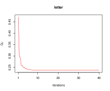
(a) letter

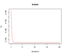
(b) breast

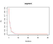
(c) segment

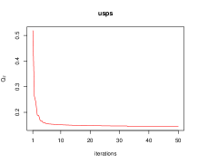
(d) usps

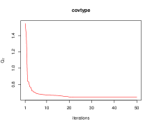
(e) covtype

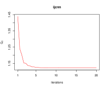
(f) ijcnn

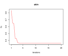
(g) skin

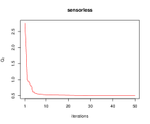
(h) sensorless

Figure 1: The reported $Q_{F}$ as a function of iterations. As the number of iterations increases, $Q_{F}$ monotonically decreases and converges.

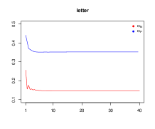
(a) letter

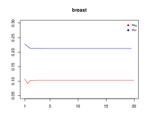
(b) breast

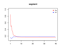
(c) segment

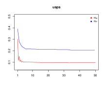
(d) usps

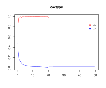
(e) covtype

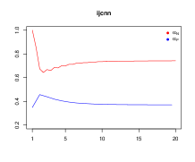
(f) ijcnn

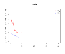
(g) skin

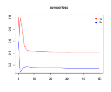
(h) sensorless

Figure 2: The value of $\alpha_{P}$ (red line) and $\alpha_{N}$ (blue line) obtained as a function of iterations. Both of them are convergent for each dataset.

Table 6: The running time (in seconds) with different algorithms for imbalanced classification problems.

Dataset	MPMF	Plug-in	SVM	ROS	SMOTE	ADASYN	RUS	CC	BRF	RUSBoost	KMPMF
letter	0.1878	0.1419	0.1346	0.9458	0.9115	1.1413	0.0151	58.796	1.0127	2.0387	6.0161
breast	0.0550	0.0021	0.0018	0.0039	0.0047	0.0079	0.0024	2.9232	0.3917	0.7886	1.2615
segment	0.2984	0.0280	0.0152	0.0739	0.0710	0.0985	0.0074	6.0516	0.6517	1.0120	5.6141
usps	1.4405	24.088	0.7531	2.5059	2.3554	5.9611	0.1479	124.67	1.9727	10.271	18.138
covtype	0.3504	9.4688	33.317	41.966	1201.6	2820.2	21.513	-	163.56	290.15	457.27
ijcnn	0.1082	0.3404	0.9117	2.5844	2.9956	8.4936	0.1421	1923.4	5.1220	10.891	28.282
skin	0.2455	0.6936	3.8266	7.8850	8.1759	8.9347	1.7048	-	17.873	35.793	22.468
sensorless	0.5073	7.9259	4.6929	10.856	12.336	14.781	0.6054	1021.8	4.0356	12.928	36.127

Table 7: The value of the F1-measure obtained with different algorithms for imbalanced classification problems.

Dataset	MPMF	Plug-in	SVM	ROS	SMOTE	ADASYN	RUS	CC	BRF	RUSBoost	KMPMF
letter	0.5361	0.6122	0.4539	0.4188	0.4252	0.3338	0.4083	0.4035	0.7548	0.6021	0.8934
breast	0.9676	0.9467	0.9477	0.9514	0.9480	0.9524	0.9540	0.9477	0.9620	0.9319	0.9772
segment	0.8516	0.8899	0.7995	0.7870	0.7958	0.7640	0.7579	0.7566	0.9176	0.8982	0.9105
usps	0.8533	0.8396	0.8745	0.8442	0.8547	0.8305	0.7887	0.7663	0.8753	0.7813	0.9011
covtype	0.7105	0.7091	0.6783	0.7107	0.7120	0.7016	0.7106	-	0.9506	0.7181	0.6718
ijcnn	0.5524	0.5967	0.4178	0.5136	0.5228	0.5048	0.5212	0.2913	0.7693	0.6411	0.6269
skin	0.8839	0.8442	0.8213	0.8634	0.8642	0.8344	0.8629	-	0.9979	0.9167	0.9938
sensorless	0.6009	0.5860	0.2150	0.5351	0.5351	0.4641	0.5154	0.4857	0.9842	0.9681	0.9198

7 Conclusion

In many real-world problems, only the mean and covariance matrix but not the true distribution of data are known in advance. To address this issue, [29] proposed the minimax probability machine (MPM) based on the mean and covariance matrix of data and the accuracy rate. However, the accuracy rate is not an appropriate metric for imbalanced classification problems. In this paper, we extended MPM to deal with imbalance classification problems based on some non-decomposable performance measures including the $F_{\beta}$ measure for the first time. To solve the new model effectively, we derived its equivalent minimization formulation in terms of a polynomial combination of FPR and FNR, which is then solved by using the alternating descent method. The kernel trick is also used to obtain a nonlinear $F_{\beta}$ maximization. The advantage of our method is that it makes use of only the mean and covariance matrix of data and thus is independent of the training data size, so our method is also appropriate for large-scale problems. In addition, our method has no hyper-parameters to choose. Experiments on both the synthetic dataset and real-world benchmark datasets have been presented to illustrate the effectiveness of our method.

It is noted that certain online learning algorithms have also been studied recently for the $F_{\beta}$-measure [38, 4, 32] to handle large-scale problems. As an ongoing project, we are currently developing certain online learning algorithms based on non-decomposable performance measures including the $F_{\beta}$-measure which can deal with imbalanced large-scale problems. In addition, deep networks have recently been applied to non-decomposable measure maximization problems [43]. Note that our method is not very efficient in dealing with very high-dimensional imbalanced classification problems due to the large storage requirement to store the estimator of the true covariance matrix of data. One way to overcome this difficulty is to use a dimension reduction method to reduce the feature dimensions of data. We hope to study these topics in the near future.

References

- [1] K. Bascol, R. Emonet, E. Fromont, A. Habrard, G. Metzler, and M. Sebban. From cost-sensitive classification to tight F-measure bounds. In International Conference on Artificial Intelligence and Statistics, pages 1245–1253, Naha, Okinawa, Japan, April 2019.
- [2] D. Bertsimas and I. Popescu. Optimal inequalities in probability theory: A convex optimization approach. SIAM Journal on Optimization, 15(3):780–804, 2005.
- [3] S. Boyd and L. Vandenberghe. Convex Optimization. Cambridge University Press, New York, NY, United States, 2004.
- [4] R. Busa-Fekete, B. Szörényi, K. Dembczyński, and E. Hüllermeier. Online F-measure optimization. In Advances in Neural Information Processing Systems, pages 595–603, Montréal, Canada, December 2015.
- [5] A. Cano, A. Zafra, and S. Ventura. Weighted data gravitation classification for standard and imbalanced data. IEEE Transactions on Cybernetics, 43(6):1672–1687, December 2013.
- [6] N. Chawla, K. Bowyer, L. Hall, and W. Kegelmeyer. Smote: synthetic minority over-sampling technique. Journal of Artificial intelligence Research, 16:321–357, 2002.
- [7] C. Chen, A. Liaw, and L. Breiman. Using random forest to learn imbalanced data. University of California, Berkeley, pages 1–12, 2004.
- [8] P. Chinta, P. Balamurugan, S. Shevade, and M. Murty. Optimizing F-measure with non-convex loss and sparse linear classifiers. In International Joint Conference on Neural Networks, pages 2858–2865, Dallas, United States, August 2013.
- [9] S. Cousins and J. Shawe-Taylor. High-probability minimax probability machines. Machine Learning, 106(6):863–886, 2017.
- [10] K. Dembczyński, W. Kotlowski, O. Koyejo, and N. Natarajan. Consistency analysis for binary classification revisited. In the 34th International Conference on Machine Learning, pages 961–969, Sydney, Australia, August 2017.
- [11] K. Dembczyński, W. Waegeman, W. Cheng, and E. Hüllermeier. An exact algorithm for F-measure maximization. In Advances in Neural Information Processing Systems, pages 1404–1412, Granada, Spain, December 2011.
- [12] E. Eban, M. Schain, A. Mackey, A. Gordon, R. Saurous, and G. Elidan. Scalable learning of non-decomposable objectives. In the 20th International Conference on Artificial Intelligence and Statistics, pages 832–840, Fort Lauderdale, United States, April 2017.
- [13] H. Guo, Y. Li, J. Shang, M. Gu, Y. Huang, and B. Gong. Learning from class-imbalanced data: Review of methods and applications. Expert Systems with Applications, 73:220–239, May 2017.
- [14] H. He, Y. Bai, E. Garcia, and S. Li. Adasyn: Adaptive synthetic sampling approach for imbalanced learning. In IEEE International Joint Conference on Neural Networks, pages 1322–1328, 2008.
- [15] H. He and E. Garcia. Learning from imbalanced data. IEEE Transactions on Knowledge and Data Engineering, 21(9):1263–1284, September 2009.
- [16] J. Hu, H. Yang, M. Lyu, I. King, and A. So. Online nonlinear auc maximization for imbalanced data sets. IEEE Transactions on Neural Networks and Learning Systems, 29(4):1253–1286, April 2018.
- [17] K. Huang, H. Yang, I. King, and M. Lyu. Imbalanced learning with a biased minimax probability machine. IEEE Transactions on Systems, Man, and Cybernetics-part B: Cybernetics, 36(4):913–923, August 2006.
- [18] K. Huang, H. Yang, I. King, M. Lyu, and L. Chan. Biased minimax probability machine for medical diagnosis. In International Symposium on Artificial Intelligence and Mathematics, Florida, United States, January 2004.
- [19] K. Huang, H. Yang, I. King, M. Lyu, and L. Chan. The minimum error minimax probability machine. Journal of Machine Learning Research, 5:1253–1286, 2004.
- [20] M. Jansche. Maximum expected F-measure training of logistic regression models. In the Human Language Technology Conference and the Conference on Empirical Methods in Natural Language Processing, pages 692–699, 2005.
- [21] M. Jansche. A maximum expected utility framework for binary sequence labeling. In the Annual Meetings of the Association for Computational Linguistics, pages 736–743, Prague, Czech Republic, June 2007.
- [22] T. Joachims. A support vector method for multivariate performance measures. In Proceedings of the International Conference on Machine Learning, pages 377–384, Bonn, Germany, August 2005.
- [23] J. Johnson and T. Khoshgoftaar. Survey on deep learning with class imbalance. Journal of Big Data, 6(27):4152–4165, September 2019.
- [24] Q. Kang, L. Shi, M. Zhou, X. Wang, Q. Wu, and Z. Wei. A distance-based weighted undersampling scheme for support vector machines and its application to imbalanced classification. IEEE Transactions on Neural Networks and Learning Systems, 29(9):4152–4165, September 2018.
- [25] S. Khan, M. Hayat, M. Bennamoun, F. Sohel, and R. Togneri. Cost-sensitive learning of deep feature representations from imbalanced data. IEEE Transactions on Neural Networks and Learning Systems, 29(8):3573 –3587, August 2018.
- [26] W. Kotlowski and K. Dembczyński. Surrogate regret bounds for generalized classification performance metrics. Machine Learning, 106:549–572, October 2017.
- [27] O. Koyejo, N. Natarajan, P. Ravikumar, and I. Dhillon. Consistent binary classification with generalized performance metrics. In Advances in Neural Information Processing Systems, pages 2744–2752, Montréal, Canada, December 2014.
- [28] B. Krawczyk, M. Koziarski, and M. Wozniak. Radial-based oversampling for multiclass imbalanced data classification. IEEE Transactions on Neural Networks and Learning Systems, 31(8):2818–2831, 2020.
- [29] G. Lanckriet, L. Ghaoui, C. Bhattacharyya, and M. Jordan. A robust minimax approach to classification. Journal of Machine Learning Research, 3:555–582, 2002.
- [30] G. Lemaitre, F. Nogueira, and C. Aridas. Imbalanced-learn: A python toolbox to tackle the curse of imbalanced datasets in machine learning. Journal of Machine Learning Research, 18:1–5, 2017.
- [31] D. Lewis. Evaluating and optimizing autonomous text classification systems. Proceedings of the 18th annual international ACM SIGIR conference on Research and development in information retrieval, pages 246–254, July 1995.
- [32] M. Liu, X. Zhang, X. Zhou, and T. Yang. Faster online learning of optimal threshold for consistent F-measure optimization. In Advances in Neural Information Processing Systems, pages 3889–3899, Montréal, Canada, December 2018.
- [33] A. Marshall and Olkin. Multivariate chebyshev inequalities. Annals of Mathematical Statistics, 31:1001–1014, 1960.
- [34] J. Mathew, C.K. Pang, M. Luo, and W.H. Leong. Classification of imbalanced data by oversampling in kernel space of support vector machines. IEEE Transactions on Neural Networks and Learning Systems, 29(9):4065–4076, 2018.
- [35] A. Menon, H. Narasimhan, S. Agarwal, and S. Chawla. On the statistical consistency of algorithms for binary classification under class imbalance. In Proceedings of the International Conference on Machine Learning, pages 603–611, Atlanta, USA, June 2013.
- [36] D. Musicant, V. Kumar, and A. Ozgur. Optimizing F-measure with support vector machines. In Proceedings of the 16th International Florida Artificial Intelligence Research Society Conference, pages 356–360, 2003.
- [37] H. Narasimhan, A. Cotter, and M. Gupta. Optimizing generalized rate metrics with three players. In Advances in Neural Information Processing Systems, pages 10747–10758, Vancouver, Canada, December 2019.
- [38] H. Narasimhan, P. Kar, and P. Jain. Optimizing non-decomposable performance measures: A tale of two classes. In Proceedings of the International Conference on Machine Learning, pages 199–208, Lille, France, July 2015.
- [39] H. Narasimhan, R. Vaish, and S. Agarwal. On the statistical consistency of plug-in classifiers for non-decomposable performance measures. In Advances in Neural Information Processing Systems, pages 1493–1501, Montréal, Canada, December 2014.
- [40] N. Natarajan, O. Koyejo, P. Ravikumar, and I. Dhillon. Optimal decision-theoretic classification using non-decomposable performance metrics. arXiv:1505.01802, 2015.
- [41] S. Parambath, N. Usunier, and Y. Grandvalet. Optimizing F-measures by cost-sensitive classification. In Advances in Neural Information Processing Systems, pages 2123–2131, Montréal, Canada, December 2014.
- [42] F. Pedregosa, G. Varoquaux, A. Gramfort, V. Michel, B. Thirion, O. Grisel, M. Blondel, P. Prettenhofer, R. Weiss, V. Dubourg, J. Vanderplas, A. Passos, D. Cournapeau, M. Brucher, M. Perrot, and E. Duchesnay. Scikit-learn: Machine learning in Python. Journal of Machine Learning Research, 12:2825–2830, 2011.
- [43] A. Sanyal, P. Kumar, P. Kar, S. Chawla, and F. Sebastiani. Optimizing non-decomposable measures with deep networks. Machine Learning, 108:1597–1620, July 2018.
- [44] C. Seiffert, T. Khoshgoftaar, J. Hulse, and A. Napolitano. Rusboost: a hybrid approach to alleviating class imbalance. IEEE Transactions on Systems, Man, and Cybernetics-Part A: Systems and Humans, 40(1):185–197, 2009.
- [45] W. Waegeman, K. Dembczyński, A. Jachnik, W. Cheng, and E. Hüllermeier. On the Bayes-optimality of F-measure maximizers. Journal of Machine Learning Research, 15:3333–3388, 2014.
- [46] N. Ye, K. Chai, W. Lee, and H. Chieu. Optimizing F-measures: A tale of two approaches. In Proceedings of the International Conference on Machine Learning, pages 1555–1562, Edinburgh, Scotland, June 2012.
- [47] Z. Zhu, Z. Wang, D. Li, Y. Zhu, and W. Du. Geometric structural ensemble learning for imbalanced problems. IEEE Transactions on Cybernetics, 50(4):1617–1629, April 2020.