Abstract

We examine the general problem of inter-domain Gaussian Processes (GPs): problems where the GP realization and the noisy observations of that realization lie on different domains. When the mapping between those domains is linear, such as integration or differentiation, inference is still closed form. However, many of the scaling and approximation techniques that our community has developed do not apply to this setting. In this work, we introduce the hierarchical inducing point GP (HIP-GP), a scalable inter-domain GP inference method that enables us to improve the approximation accuracy by increasing the number of inducing points to the millions. HIP-GP, which relies on inducing points with grid structure and a stationary kernel assumption, is suitable for low-dimensional problems. In developing HIP-GP, we introduce (1) a fast whitening strategy, and (2) a novel preconditioner for conjugate gradients which can be helpful in general GP settings. Our code is available at https://github.com/cunningham-lab/hipgp.

1 INTRODUCTION

Gaussian processes (GPs) are a widely used statistical tool for inferring unobserved functions (Cressie,, 1992, 1990; Rasmussen and Williams,, 2006). The classic goal of GPs is to infer the unknown function given noisy observations. Here, we are interested in a more general setting, inter-domain GPs, where the observed data is related to the latent function via some linear transformation, such as integration or differentiation, while an identity transformation recovers the standard GP problem. One motivating example is an astrophysics problem: mapping the three-dimensional spatial distribution of dust in the Milky way (Green et al.,, 2015; Leike and Enßlin,, 2019; Kh et al.,, 2017). Interstellar dust is a latent function that can be inferred from star observations. However, because we are embedded in our own dust field, we can only observe some noisy integral of the dust function along the line of sight between Earth and a star. Beyond this example, inter-domain GPs arise often in the literature: integrated observations have been used in probabilistic construction of optimization algorithms (Wills and Schön,, 2017), quadrature rules (Minka,, 2000), and tomographic reconstructions (Jidling et al.,, 2018); while derivative observations have been used in dynamical systems (Solak et al.,, 2003), modeling monotonic functions (Riihimäki and Vehtari,, 2010) and Bayesian optimization (Garnett et al.,, 2010; Siivola et al.,, 2018).

In practice, this type of inter-domain GP problem poses two interwined obstacles that are beyond the reach of current techniques. First, large-scale exact modeling is usually intractable. The joint distribution of inter-domain observations and the underlying GP involves the transformed-domain and inter-domain kernel expressions, which rarely admits analytical solutions and requires approximations (Lázaro-Gredilla and Figueiras-Vidal,, 2009; Hendriks et al.,, 2018). Common approximations are often handled by numerical integration, which is infeasible for big datasets since it requires integrating all pairwise correlations.

Moreover, inter-domain GPs suffer from the same scalability issues as regular GPs. For a dataset with $N$ observations, the likelihood function depends on $N^{2}$ pairwise correlations. The leading strategy to scale standard GP inference is to use $M\ll N$ inducing points to represent the global behavior of GP functions (Rasmussen and Williams,, 2006). One popular inducing point method is stochastic variational Gaussian process (SVGP), which factorizes the objective over mini-batches of data and requires only $O(M^{2})$ storage and $O(M^{3})$ computation (Hensman et al.,, 2013). In the current practice of SVGP, $M$ is limited to under $10{,}000$ (Wilson and Nickisch,, 2015; Izmailov et al.,, 2018). However, many inter-domain problems are spatial or temporal in nature, and the data do not lie in some small manifold in that space. In the interstellar dust problem, for example, we aim to make inference at every point in a dense 3D space. A small set of inducing points is incapable of resolving the resolution of interest, which is around 4 orders of magnitude smaller than the domain size. Furthermore, Bauer et al., (2016) shows that more inducing points are needed to reduce the overestimated observation noise parameter induced by SVGP. All of these facts necessitate the need to scale both $N$ and $M$ to larger quantities.

To this end, we develop the hierarchical inducing point GP (HIP-GP), a method to scale GP inference to millions of inducing points and observations for spatial-temporal inter-domain problems. In particular,

• We adapt the SVGP framework to inter-domain settings by decoupling observations and inducing points into different domains. This framework alleviates the difficulties of computing the full transformed kernel matrices, and enables the exploitations of the latent kernel structure.

• We then develop the HIP-GP algorithm to address the computational bottlenecks of standard SVGP objectives, employing two core strategies:

  • Fast matrix inversion with conjugate gradient method using the hierachical Toeplitz structure. Upon this structure, we design a novel preconditioner and a new whitening strategy to further speed up computations;

  • A structured variational approximation of the posterior over inducing point values.

HIP-GP is suitable for low-dimensional inter-domain GP problems, and applies in settings where the kernel function is stationary and inducing points fall on a fixed, evenly-spaced grid. In addition, the technical innovations in developing HIP-GP are useful in a variety of more general settings.

2 BACKGROUND

2.1 Inter-domain GPs

Following the notations in van der Wilk et al., (2020), we consider a statistical model of the form

$$\rho \sim GP\left(0,k_{\theta}(\cdot,\cdot)\right)$$ (1)

$$\rho^{*} =\mathcal{L}\circ\rho$$ (2)

$$y_{n}\,|\,\boldsymbol{x}_{n},\rho^{*} \sim\mathcal{N}(\rho^{*}(\boldsymbol{x}_{n}),\sigma_{n}^{2})$$ (3)

for a dataset of $N$ observations $\mathcal{D}\triangleq\{y_{n},\boldsymbol{x}_{n},\sigma_{n}^{2}\}_{n=1}^{N}$, where $\mathcal{L}$ is a linear operator and $k_{\theta}(\cdot,\cdot)$ is the covariance function that encodes prior assumptions about the function $\rho$. Note that GPs are closed under linear operators, therefore $\rho^{*}$ is also a GP (Rasmussen and Williams,, 2006).

One common linear operator is the integral operator, $\mathcal{L}\circ\rho(\cdot)=\int\rho(\boldsymbol{x})w(\boldsymbol{x})d\boldsymbol{x}$, as used in Lázaro-Gredilla and Figueiras-Vidal, (2009). We see that this $\mathcal{L}$ maps the entire function $\rho(\cdot)$ to a single real value. Another example is the derivative of the $d$th input dimension $\mathcal{L}\circ\rho(\cdot)=\frac{\partial\rho}{\partial x_{d}}(\boldsymbol{x}_{n})$. In this case, the operator only depends on the neighborhood around $\boldsymbol{x}_{n}$. Derivative observations are often useful for algorithmic purposes, e.g. in Riihimäki and Vehtari, (2010). In application problems, they could be either collected, e.g. velocity measured by physical detectors, or identified from function observations (Solak et al.,, 2003). We also notice that setting $\mathcal{L}$ to an identity map fits regular GPs into this framework.

The goal of inter-domain GPs is to infer the underlying function $\rho(\boldsymbol{x})$ — either to compute $p(\rho(\boldsymbol{x}_{*})\,|\,\mathcal{D})$ for new test locations $\boldsymbol{x}_{*}$ or to improve estimates of $p(\rho(\boldsymbol{x}_{n})\,|\,\mathcal{D})$ for observed location $\boldsymbol{x}_{n}$ given all observations.

2.2 Stochastic Variational Gaussian Process

The stochastic variational Gaussian process (SVGP) is an approximate method that scales GP inference to large $N$ (Hensman et al.,, 2013). Denote the $M$ inducing point locations $\bar{\boldsymbol{x}}=\left(\bar{\boldsymbol{x}}_{1},\dots,\bar{\boldsymbol{x}}_{M}\right)$, and the vector of inducing point values $\boldsymbol{u}\triangleq\left(\rho(\bar{\boldsymbol{x}}_{1}),\dots,\rho(\bar{\boldsymbol{x}}_{M})\right)$. SVGP defines a variational distribution over the inducing point values $\boldsymbol{u}$ and the latent process values $\boldsymbol{\rho}\triangleq\left(\rho(\boldsymbol{x}_{1}),\dots,\rho(\boldsymbol{x}_{N})\right)$ of the form

$$q(\boldsymbol{u},\boldsymbol{\rho})=q_{{\boldsymbol{\lambda}}}(\boldsymbol{u})p(\boldsymbol{\rho}\,|\,\boldsymbol{u})\,,\quad q_{{\boldsymbol{\lambda}}}(\boldsymbol{u})=\mathcal{N}(\boldsymbol{u}\,|\,\boldsymbol{m},\boldsymbol{S})\,,$$

where $q_{\boldsymbol{\lambda}}(\boldsymbol{u})$ is a multivariate Gaussian, $p(\boldsymbol{\rho}\,|\,\boldsymbol{u})$ is determined by the GP prior and ${\boldsymbol{\lambda}}\triangleq(\boldsymbol{m},\boldsymbol{S})$ are variational parameters. This choice of variational family induces a convenient cancellation, resulting in a separable objective (Titsias,, 2009)

$$\mathcal{L}({\boldsymbol{\lambda}})$$ (4)

$$=\underbrace{\mathbb{E}_{q_{{\boldsymbol{\lambda}}}(\boldsymbol{u})}\left[\mathbb{E}_{p(\boldsymbol{\rho}\,|\,\boldsymbol{u})}\left[\ln p(\boldsymbol{y}\,|\,\boldsymbol{\rho})\right]\right]}_{\leavevmode\hbox to5.02pt{\vbox to5.02pt{\text{[drawing]}}}}-\underbrace{KL(q_{{\boldsymbol{\lambda}}}(\boldsymbol{u})\,||\,p(\boldsymbol{u}))}_{\leavevmode\hbox to6.62pt{\vbox to6.62pt{\text{[drawing]}}}}\,.$$

We can write as a sum over $N$ observations

$$=\sum_{n=1}^{N}\underbrace{\mathbb{E}_{q_{{\boldsymbol{\lambda}}}(\boldsymbol{u})}\left[\mathbb{E}_{p(\rho_{n}\,|\,\boldsymbol{u})}\left[\ln p(y_{n}\,|\,\rho_{n})\right]\right]}_{\triangleq\leavevmode\hbox to7.57pt{\vbox to7.57pt{\text{[drawing]}}}}\,. a_{n} a_{n}$$ (5)

The factorization of enables the objectives to be estimated with mini-batches in a large dataset. However, notice that , the KL-divergence of two Gaussians, will involve a term $\ln|\boldsymbol{K}_{\boldsymbol{u},\boldsymbol{u}}|$ which requires $O(M^{3})$ computation.

2.3 Matrix Solves with Conjugate Gradients

Conjugate gradients (CG) is an iterative algorithm for solving a linear system using only matrix-vector multiplies (MVM). CG computes $\boldsymbol{K}^{-1}\boldsymbol{p}$ for any $\boldsymbol{p}\in\mathbb{R}^{M}$ by computing $\boldsymbol{K}\boldsymbol{v}$ for a sequence of vectors $\boldsymbol{v}\in\mathbb{R}^{M}$ determined by the algorithm. For $\boldsymbol{K}$ of size $M\times M$, CG computes the exact solution after $M$ iterations, and typically converges after some smaller number of steps $S<M$ (Hestenes and Stiefel,, 1952; Nocedal and Wright,, 2006).

Preconditioned conjugate gradients (PCG) is an augmented version of CG that solves the system in a transformed space. A good preconditioner can dramatically speed up convergence (Shewchuk et al.,, 1994; Cutajar et al.,, 2016).

3 SCALING $M$: HIP-GP for INTER-DOMAIN PROBLEMS

We first formulate the SVGP framework for inter-domain observations, and identify its computational bottlenecks in Section 3.1. We then address these bottlenecks by the HIP-GP algorithm using the techniques developed in Section 3.2 - 3.3. In Section 3.4, we summarize our methods and discuss optimization procedures for HIP-GP.

3.1 Inter-domain SVGP Formulation

We show that the inter-domain observations can be easily incorporated into the SVGP framework. We place a set of inducing points $\boldsymbol{u}=\rho(\bar{\boldsymbol{x}})$ in the latent domain at input locations $\bar{\boldsymbol{x}}=\left(\bar{\boldsymbol{x}}_{1},\cdots,\bar{\boldsymbol{x}}_{M}\right)$. Connections to the observations are made through the inter-domain covariance, while the observations are characterized by the transformed-domain covariance. Formally, we have the inter-domain GP prior:

$$\begin{pmatrix}\rho_{n}^{*}\\ \boldsymbol{u}\end{pmatrix}\sim\mathcal{N}\left(0,\begin{pmatrix}k^{**}_{n,n}&\boldsymbol{k}^{*}_{n,\boldsymbol{u}}\\ \boldsymbol{k}^{*}_{\boldsymbol{u},n}&\boldsymbol{K}_{\boldsymbol{u},\boldsymbol{u}}\\ \end{pmatrix}\right),$$ (6)

where the inter-domain covariance and the transformed-domain covariance are defined as

$$\boldsymbol{k}^{*}_{\boldsymbol{u},n} \triangleq Cov\left(\rho(\bar{\boldsymbol{x}}),\rho^{*}(\boldsymbol{x}_{n})\right)=Cov\left(\boldsymbol{u},\rho^{*}_{n}\right)\,,$$ (7)

$$k^{**}_{n,n} \triangleq Cov\left(\rho^{*}(\boldsymbol{x}_{n}),\rho^{*}(\boldsymbol{x}_{n})\right)=Cov\left(\rho^{*}_{n},\rho^{*}_{n}\right)\,,$$ (8)

and the latent domain covariance is

$$\boldsymbol{K}_{\boldsymbol{u},\boldsymbol{u}} \triangleq Cov\left(\rho(\bar{\boldsymbol{x}}),\rho(\bar{\boldsymbol{x}})\right)=Cov\left(\boldsymbol{u},\boldsymbol{u}\right).$$ (9)

This form of the prior suggests formulating the inter-domain SVGP objective as follows

$$\mathcal{L}({\boldsymbol{\lambda}}) =\sum_{n=1}^{N}\mathbb{E}_{q_{{\boldsymbol{\lambda}}}(\boldsymbol{u})}\left[\mathbb{E}_{p(\rho_{n}^{*}\,|\,\boldsymbol{u})}\left[\ln p(y_{n}\,|\,\rho_{n}^{*})\right]\right]$$ (10)

$$\qquad-KL(q_{{\boldsymbol{\lambda}}}(\boldsymbol{u})\,||\,p(\boldsymbol{u}))\,,$$

where

$$p(\rho_{n}^{*}|\boldsymbol{u}) =N(\rho_{n}^{*}|\boldsymbol{k}_{n,\boldsymbol{u}}^{*}\boldsymbol{K}_{\boldsymbol{u},\boldsymbol{u}}^{-1}\boldsymbol{u},k_{n,n}^{**}-\boldsymbol{k}_{n,\boldsymbol{u}}^{*}\boldsymbol{K}_{\boldsymbol{u},\boldsymbol{u}}^{-1}\boldsymbol{k}_{\boldsymbol{u},n}^{*})\,.$$

Note that this framework can be extended to observations in multiple domains by including them with their corresponding inter-domain and transformed-domain covariances. Under this formulation, we avoid computing the $N\times N$ transformed-domain covariance matrix $\boldsymbol{K}_{N,N}^{**}$ that appears in the exact GP objective. Instead, only $N$ terms of variance $k_{n,n}^{**}$ need to be evaluated. Importantly, the disentanglement of observed and latent domains enables us to exploit structure of $\boldsymbol{K}_{\boldsymbol{u},\boldsymbol{u}}$ for efficient computations. Such exploitation would be difficult without a variational approximation, especially in the case of mixed observations from multiple domains.

Whitened Parameterization

Whitened parameterizations are used to improve inference in models with correlated priors because they offer a better-conditioned posterior (Murray and Adams,, 2010; Hensman et al.,, 2015). Here we will show an additional computational benefit in the variational setting — the whitened posterior allows us to avoid computing $\ln|\boldsymbol{K}_{\boldsymbol{u},\boldsymbol{u}}|$ which appears in the KL term in Equation 10. To define the whitened parameterization, we describe the GP prior over $\boldsymbol{u}$ as a deterministic function of standard normal parameters $\boldsymbol{\epsilon}$:

$$\boldsymbol{\epsilon}\sim\mathcal{N}(0,I)\,,\quad\boldsymbol{u}=\boldsymbol{R}\boldsymbol{\epsilon}.$$ (11)

To preserve the covariance structure in the prior distribution of $(\rho^{*}_{n},\boldsymbol{u})$ (Equation 6), the transformation $\boldsymbol{R}$ and the whitened correlation $\boldsymbol{k}_{n}\triangleq Cov(\boldsymbol{\epsilon},\rho^{*}_{n})$ need to satisfy the following two equalities:

$$\boldsymbol{K}_{\boldsymbol{u},\boldsymbol{u}} =Cov(\boldsymbol{R}\boldsymbol{\epsilon},\boldsymbol{R}\boldsymbol{\epsilon})=\boldsymbol{R}\boldsymbol{R}^{\top}\,,$$ (12)

$$\quad\boldsymbol{k}^{*}_{\boldsymbol{u},n} =Cov(\boldsymbol{R}\boldsymbol{\epsilon},\rho^{*}_{n})=\boldsymbol{R}\boldsymbol{k}_{n}\,.$$

The classical whitening strategy in GP inference is to use the Cholesky decomposition: $\boldsymbol{K}_{\boldsymbol{u},\boldsymbol{u}}=\boldsymbol{L}\boldsymbol{L}^{\top}$ where $\boldsymbol{L}$ is a lower triangular matrix. In this case, $\boldsymbol{R}=\boldsymbol{L}$ and $\boldsymbol{k}_{n}=\boldsymbol{L}^{-1}\boldsymbol{k}^{*}_{\boldsymbol{u},n}$.

Now we can target the variational posterior over the whitened parameters $\boldsymbol{\epsilon}$: ${q_{{\boldsymbol{\lambda}}}(\boldsymbol{\epsilon})=\mathcal{N}(\boldsymbol{\epsilon}\,|\,\boldsymbol{m},\boldsymbol{S})}$. The resulting whitened variational objective is

$$\mathcal{L}({\boldsymbol{\lambda}}) =\sum_{n}\underbrace{\mathbb{E}_{q_{{\boldsymbol{\lambda}}}(\boldsymbol{\epsilon})p(\rho_{n}^{*}\,|\,\boldsymbol{\epsilon})}\left[\ln p(y_{n}\,|\,\rho_{n}^{*})\right]}_{\leavevmode\hbox to7.28pt{\vbox to7.28pt{\text{[drawing]}}}}-\underbrace{KL(q_{{\boldsymbol{\lambda}}}(\boldsymbol{\epsilon})\,||\,p(\boldsymbol{\epsilon}))}_{\leavevmode\hbox to8.18pt{\vbox to8.18pt{\text{[drawing]}}}}\, a^{\prime}_{n}$$ (13)

where

$$\quad+\boldsymbol{k}_{n}^{\intercal}\left(\boldsymbol{S}+\boldsymbol{m}\boldsymbol{m}^{\intercal}\right)\boldsymbol{k}_{n}-2y_{n}\boldsymbol{k}_{n}^{\intercal}\boldsymbol{m}\Big{)}\,\,,$$ (14)

$$=\frac{1}{2}\left(\text{tr}(\boldsymbol{S})+\boldsymbol{m}^{\intercal}\boldsymbol{m}-\ln|\boldsymbol{S}|-M\right).$$ (15)

Computational Bottlenecks

The whitened objective above still factorizes over data points. However, there remain two computational bottlenecks. First, the correlation term $\boldsymbol{k}_{n}$ in depends on the choice of the whitening strategy. The common Cholesky strategy requires $O(M^{3})$ computation and $O(M^{2})$ storage which is infeasible for large $M$. We address this bottleneck in Section 3.2. The second bottleneck lies in the variational covariance $\boldsymbol{S}$ which is an $M\times M$ matrix, requiring $O(M^{2})$ to store and $O(M^{3})$ to compute the $\ln|\boldsymbol{S}|$ in . We will address this problem by a structured variational approximation in Section 3.3.

3.2 Computational Accelerations

We now turn to the first bottleneck — how to design an efficient whitening strategy to compute the term $\boldsymbol{k}_{n}$. To do so, we rely on judicious placement of inducing points and assume a stationary covariance function, a general and commonly used class. We describe three key ingredients below.

Hierarchical Toeplitz Structure

Consider a $D$-dimensional grid of evenly spaced points of size $M\triangleq M_{1}\times\cdots\times M_{D}$, characterized by one-dimensional grids of size $M_{i}$ along dimension $i,i=1:D$, where $D$ is the input dimension. Under a stationary kernel, we construct a covariance matrix for this set of points in $x$-major order (i.e. C-order). Such a matrix will have hierarchical Toeplitz structure, which means the diagonals of the matrix are constant. Because of this data redundancy, a hierarchical Toeplitz matrix is characterized by its first row. Now we place the inducing points along a fixed, equally-spaced grid, resulting in a $M\times M$ hierarchical Toeplitz Gram matrix $\boldsymbol{K}_{\boldsymbol{u},\boldsymbol{u}}$. The efficient manipulation of $\boldsymbol{K}_{\boldsymbol{u},\boldsymbol{u}}$ is through its circulant embedding:

$$\boldsymbol{C}=\begin{pmatrix}\boldsymbol{K}_{\boldsymbol{u},\boldsymbol{u}}&\tilde{\boldsymbol{K}}\\ \tilde{\boldsymbol{K}}^{\top}&\boldsymbol{K}_{\boldsymbol{u},\boldsymbol{u}}\end{pmatrix}$$ (16)

where $\tilde{\boldsymbol{K}}$ is the appropriate reversal of $\boldsymbol{K}_{\boldsymbol{u},\boldsymbol{u}}$ to make $\boldsymbol{C}$ circulant. $\boldsymbol{C}$ admits a convenient diagonalization

$$\boldsymbol{C}=\boldsymbol{F}^{\top}\boldsymbol{D}\boldsymbol{F}=\boldsymbol{F}^{\top}\text{diag}\left(\boldsymbol{F}\boldsymbol{c}\right)\boldsymbol{F}\,\,,$$ (17)

where $\boldsymbol{F}$ is the fast Fourier transform matrix, $\boldsymbol{D}$ is a diagonal matrix of $\boldsymbol{C}$’s eigenvalues, and $\boldsymbol{c}$ is the first row of $\boldsymbol{C}$. This diagonalization enables fast MVMs with $\boldsymbol{C}$ and hence the embedded $\boldsymbol{K}_{\boldsymbol{u},\boldsymbol{u}}$ via the FFT algorithm in $O(M\ln M)$ time, further making it sufficient for use within CG to efficiently solve a linear system.

The fast solves afforded by Toeplitz structure have been previously utilized for exact GP inference (Cunningham et al.,, 2008; Wilson et al.,, 2015). Here, we extend the applicability of Toeplitz structure to the variational inter-domain case by introducing a fast whitening procedure and an effective preconditioner for CG.

Fast Whitening Strategy

Similar to the Cholesky decomposition, we aim to find a whitened matrix $\boldsymbol{R}$ that serves as a root of $\boldsymbol{K}_{\boldsymbol{u},\boldsymbol{u}}$, i.e. $\boldsymbol{R}\boldsymbol{R}^{T}=\boldsymbol{K}_{\boldsymbol{u},\boldsymbol{u}}$. Directly solving $\boldsymbol{K}_{\boldsymbol{u},\boldsymbol{u}}^{1/2}$ is not trivial. Alternatively, we access the root from the circulant embedding of $\boldsymbol{K}_{\boldsymbol{u},\boldsymbol{u}}$. We consider the square root of the circulant matrix

$$\boldsymbol{C}^{1/2}=\boldsymbol{F}^{\intercal}\boldsymbol{D}^{1/2}\boldsymbol{F},$$ (18)

and its block representation

$$\boldsymbol{C}^{1/2}=\begin{pmatrix}\boldsymbol{A}&\boldsymbol{B}\\ \boldsymbol{B}^{\top}&\boldsymbol{D}\\ \end{pmatrix}.$$ (19)

We make a key observation that the first row-block $(\boldsymbol{A},\boldsymbol{B})$ can be viewed as a “rectangular root” of $\boldsymbol{K}_{\boldsymbol{u},\boldsymbol{u}}$. That is, we define a non-square whitening matrix $\boldsymbol{R}$ and the correlation vector $\boldsymbol{k}_{n}$ as follows

$$\boldsymbol{R} \triangleq\begin{pmatrix}\boldsymbol{A}&\boldsymbol{B}\end{pmatrix}\,,\quad\boldsymbol{k}_{n}\triangleq\boldsymbol{R}^{T}\boldsymbol{K}_{\boldsymbol{u},\boldsymbol{u}}^{-1}\boldsymbol{k}^{*}_{\boldsymbol{u},n}.$$ (20)

One can verify such $\boldsymbol{R}$ and $\boldsymbol{k}_{n}$ satisfy Equation 12, thus offering a valid whitening strategy. We note that since $\boldsymbol{R}$ is non-square and $\boldsymbol{u}=\boldsymbol{R}\boldsymbol{\epsilon}$, this strategy doubles the number of variational parameters in each dimension of the whitened space.

Now we address how to efficiently compute $\boldsymbol{k}_{n}$ defined in Equation 20. We first compute the intermediate quantity $\boldsymbol{k}_{n}^{\prime}=\boldsymbol{K}_{\boldsymbol{u},\boldsymbol{u}}^{-1}\boldsymbol{k}^{*}_{\boldsymbol{u},n}$ via CG in $O(M\ln M)$ time. We then compute $\boldsymbol{k}_{n}=\boldsymbol{R}^{\top}\boldsymbol{k}_{n}^{\prime}$. Note that $\boldsymbol{R}^{T}$ is embedded in the matrix $\boldsymbol{C}^{1/2}$ which also admits the FFT diagonalization (Equation 18). Hence, MVM with $\boldsymbol{R}^{\top}$ can be also done in $O(M\ln M)$ time.

Lastly, we show how to make CG’s computation of $\boldsymbol{K}_{\boldsymbol{u},\boldsymbol{u}}^{-1}\boldsymbol{k}^{*}_{\boldsymbol{u},n}$ faster with a well-structured preconditioner.

Efficient Preconditioner

The ideal preconditioner $\boldsymbol{P}$ is a matrix that whitens the matrix to be inverted — the ideal $\boldsymbol{P}$ is $\boldsymbol{K}_{\boldsymbol{u},\boldsymbol{u}}^{-1}$. However, we cannot efficiently compute $\boldsymbol{K}_{\boldsymbol{u},\boldsymbol{u}}^{-1}$. But due to the convenient diagonalization of the circulant embedding matrix $\boldsymbol{C}$, we can efficiently compute the inverse of $\boldsymbol{C}$:

$$\boldsymbol{C}^{-1}=\boldsymbol{F}^{\top}\boldsymbol{D}^{-1}\boldsymbol{F}\,.$$ (21)

Note that the upper left block of $\boldsymbol{C}^{-1}$ does not correspond to $\boldsymbol{K}_{\boldsymbol{u},\boldsymbol{u}}^{-1}$ as we explicitly write out

$$\boldsymbol{C}^{-1}=\begin{pmatrix}\left(\boldsymbol{K}_{\boldsymbol{u},\boldsymbol{u}}-\tilde{\boldsymbol{K}}\boldsymbol{K}_{\boldsymbol{u},\boldsymbol{u}}^{-1}\tilde{\boldsymbol{K}}^{\intercal}\right)^{-1}&...\quad\\ ...&...\quad\end{pmatrix}\,\,.$$ (22)

However, when the number of inducing points are large enough, $\boldsymbol{K}_{\boldsymbol{u},\boldsymbol{u}}$ approaches a banded matrix, and so $\tilde{\boldsymbol{K}}$ is increasingly sparse. Therefore, the upper left block of $\boldsymbol{C}^{-1}$ would be close to $\boldsymbol{K}_{\boldsymbol{u},\boldsymbol{u}}^{-1}$, suggesting that it can serve as an effective preconditioner within PCG, and therefore an effective strategy for solving a linear system with the kernel matrix. We note that this banded property is often exploited in developing effective preconditioners (Chan and Ng,, 1996; Saad,, 2003). To justify this intuition, we anlayze the PCG convergence speed under various settings of kernel functions and inducing point densities in appendix. We compare the performance of PCG and CG in systems of varying size in Section 5.1. We find that PCG converges faster than CG across all systems, taking only a fraction of the number of iterations that standard CG requires to converge. This speedup is crucial — PCG is a subroutine we use to compute the gradient term corresponding to each observation $n$.

Summary of Fast Computation for $\boldsymbol{k}_{n}$

To summarize, we exploit additional computational benefits of the hierarchical Toeplitz matrix through its circulant embedding matrix, which enables fast matrix square-root and matrix inverse. We further utilize these fast operations to design novel whitening and preconditioning strategies. Thus, the whitened correlation term $\boldsymbol{k}_{n}=\boldsymbol{R}^{T}\boldsymbol{K}_{\boldsymbol{u},\boldsymbol{u}}^{-1}\boldsymbol{k}^{*}_{\boldsymbol{u},n}$ can be efficiently processed as follows:

1. embed $\boldsymbol{K}_{\boldsymbol{u},\boldsymbol{u}}$ into a larger circulant matrix $\boldsymbol{C}$;

2. solve $\boldsymbol{K}_{\boldsymbol{u},\boldsymbol{u}}\boldsymbol{k}^{\prime}_{n}=\boldsymbol{k}^{*}_{\boldsymbol{u},n}$ for the intermediate term $\boldsymbol{k}^{\prime}_{n}$ with PCG, where we utilize the FFT diagonalization of $\boldsymbol{C}$ and $\boldsymbol{C}^{-1}$;

3. compute $\boldsymbol{k}_{n}=\boldsymbol{R}^{\top}\boldsymbol{k}^{\prime}_{n}$ , where we utilize the FFT diagonalization of $\boldsymbol{C}^{1/2}$.

The space and time complexity of this procedure are $O(M)$ and $O(M\ln M)$. This offers a speed-up over the Cholesky decomposition which has $O(M^{2})$ space and $O(M^{3})$ time complexity, respectively. In Section 5.2, we examine this acceleration by comparing the time of computing $\boldsymbol{k}_{n}$ using Cholesky and using HIP-GP, as the system size $M$ varying from $10^{3}$ to $10^{6}$. HIP-GP’s strategy outperforms Cholesky for small values of $M$, and scales to larger $M$ where Cholesky is no longer feasible. We present HIP-GP’s algorithmic details in appendix.

3.3 Structured Variational Approximation

Finally, we turn to the second bottleneck: how to represent and manipulate variational parameters of mean $\boldsymbol{m}$ and covariance $\boldsymbol{S}$. We propose the block independent variational family

$$q(\boldsymbol{u}) =\prod_{b}^{B}\mathcal{N}(\boldsymbol{u}_{b}\,|\,\boldsymbol{m}_{b},\boldsymbol{S}_{b})\,,$$ (23)

where $\boldsymbol{u}_{b}$ denotes a subset of inducing points of size $M_{b}<M$ and $\boldsymbol{S}_{b}$ is the $M_{b}\times M_{b}$ variational covariance for that subset. Note that when $M_{b}=1$, it reduces to the mean-field variational family, and when $M_{b}=M$, it is the full-rank variational family. Calculations of the inverse and log-determinant of block independent $\boldsymbol{S}$ scale $O(BM_{b}^{3})$ — we must choose $M_{b}$ to be small enough to be practical.

We note that independence in the posterior is a more reasonable approximation constraint in the whitened parameterization than the original space. The original GP prior, $p(\boldsymbol{u})$, is designed to have high correlation, and therefore data are unlikely to decorrelate inducing point values. In the whitened space, on the other hand, the prior is already uncorrelated. Hence the whitened posterior is not spatially correlated as much as the original posterior. This is in addition to the benefits of optimizing in the whitened space due to better conditioning.

Constructing Blocks

The block independent approximation of Equation 23 requires assigning inducing points to $B$ blocks. Intuitively, blocks should include nearby points, and so we focus on blocks of points that tile the space. To reconcile the Toeplitz ordering and the block orderings (they may not be the same), we simply have to permute any $M$-length vector (e.g. $\boldsymbol{k}^{*}_{\boldsymbol{u},n}$ or $\boldsymbol{m}$) before multiplication with $\boldsymbol{S}$ and then undo the permutation after multiplication. Fortunately, this permutation is linear in $M$.

3.4 Method Summary

The modeling difficulty of inter-domain GP problems arises from the numerical intractability of computing the full transformed-domain covariance $\boldsymbol{K}^{**}_{N,N}$ of size $N\times N$. We avoid this difficulty by decoupling the the observations and the inducing points into different domains under the SVGP framework. Moreover, we leverage the kernel structure of the Gram matrix $\boldsymbol{K}_{\boldsymbol{u},\boldsymbol{u}}$ in the latent domain for efficient computations.

The computational difficulty stems from the computations with the kernel matrix $\boldsymbol{K}_{\boldsymbol{u},\boldsymbol{u}}$ and the variational covariance $\boldsymbol{S}$. We avoid having to compute $\ln|\boldsymbol{K}_{\boldsymbol{u},\boldsymbol{u}}|$ by using a whitened parameterization; we develop a fast whitening strategy to compute the whitened correlation term $\boldsymbol{k}_{n}=\boldsymbol{R}^{\top}\boldsymbol{K}_{\boldsymbol{u},\boldsymbol{u}}^{-1}\boldsymbol{k}^{*}_{\boldsymbol{u},n}$ by exploiting the hierarchical Toeplitz structure with a novel preconditioner; and finally we explore a structred representation for $\boldsymbol{S}$.

Optimization

We perform natural gradient descent on variational parameters using closed-form gradient updates. For gradient-based learning of kernel hyperparameters, automatically differentiating through the CG procedure is not numerically stable. Fortunately, we can efficiently compute the analytical gradient of CG solves utilizing the hierarchical Toeplitz structure, without increasing the computational complexity. See appendix for more details on gradient derivations.

4 RELATED WORK

Inter-domain GPs

The idea of the inter-domain Gaussian processes has been discussed in (Lázaro-Gredilla and Figueiras-Vidal,, 2009; van der Wilk et al.,, 2020). However, their primary interests are using inter-domain transformations to define inducing variables for specifying GP approximations, whereas our work explores the usage of SVGP framework to perform scalable modeling and inference with inter-domain observations.

Scalable Inducing Point Methods

We note several recent approaches to scaling the number of inducing points in GP approximations. Shi et al., (2020) takes an orthogonal strategy to ours by approximating GP with inducing points in two independent directions, whereas HIP-GP requires inducing points to densely cover the input space. However, while improved over standard SVGP, their method still remains a cubic complexity. Izmailov et al., (2018) introduces the tensor train decomposition into the variational approximation. Alternatively, Evans and Nair, (2018) directly approximate the kernel with a finite number of eigenfunctions evaluated on a dense grid of inducing points. Both methods rely on separable covariance kernels to utilize the Kronecker product structure. This limits the class of usable kernels. The Matérn kernel, for example, is not separable across dimensions. To fill that gap, we instead focus on the class of stationary kernels.

Another line of inducing point work is based on sparse kernel interpolations. KISS-GP uses a local kernel interpolation of inducing points to reduce both the space and time complexity to $O(N+M^{2})$ (Wilson and Nickisch,, 2015). SV-DKL also uses local kernel interpolation, and exploits separable covariance structures and deep learning techniques to address the problem of multi-output classification (Wilson et al.,, 2016). But these kernel interpolation methods are not applicable to inter-domain observations under transformations. More specifically, for standard (non-inter-domain) problems, kernel interpolation methods approximate the $N\times N$ covariance matrix $\mathbf{K}_{\mathbf{N,N}}$ with $\mathbf{W}\mathbf{K}_{\mathbf{u,u}}\mathbf{W}^{T}$, where $\mathbf{W}$ is a sparse interpolation weight matrix. However, for problems with integral observations, we must compute the integrated kernel $\mathbf{K}^{**}_{\mathbf{N,N}}=[\int\int Cov(\rho(\mathbf{x}_{i}),\rho(\mathbf{x}_{j}))d\mathbf{x}_{i}d\mathbf{x}_{j}]_{i,j=1}^{N}$. Approximating this integral with local interpolation is not straightforward, and computing every integrated cross-covariance term is costly. Alternatively, HIP-GP decouples observations and inducing points into different domains through the inter-domain prior (Equation 6). This decoupled prior enables mini-batch processing of $k_{n,n}^{**}$, eliminates the need to compute cross-covariance terms $k_{{n_{i}},{n_{j}}}^{**}$, while still maintaining structure exploitation of $\mathbf{K}_{\mathbf{u,u}}$.

Fast Whitening Strategy

As is mentioned before, the classical whitening strategy is the Cholesky decomposition that has $O(M^{2})$ space and $O(M^{3})$ time complexity. Pleiss et al., (2020) provides a more general purpose method for fast matrix roots and is in particular applicable to whitening GP. Their method is an MVM-based approach that leverages the contour integral quadrature and requires $O(M\log M+QM)$ time for $Q$ quadrature points. Our whitening strategy specifically targets gridded inducing points and achieves more complexity savings ($O(M\log M)$ time).

5 EXPERIMENTS

Due to the mismatch in missions of different scalable GP methods, we focus most of our empirical study on HIP-GP and SVGP (with Cholesky whitening) which serve the most similar purposes. We also include in appendix a standard GP problem on a UCI benchmark dataset (Dua and Graff,, 2017) where we compare HIP-GP to exact GP (Wang et al.,, 2019), sparse Gaussian Process regression (SGPR) (Titsias,, 2009) and SVGP.

5.1 Effect of the Preconditioner

We first examine the effect of the preconditioner developed in Section  3.2. We run CG and PCG with the preconditioner for systems of size $M=625~{}(25\times 25)$, $M=2{,}500~{}(50\times 50)$, and $M=10{,}000~{}(100\times 100)$ determined by a two-dimensional grid applied to the Matérn kernel. We run the algorithm to convergence (at tolerance 1e-10) for $25$ randomly initialized vectors of size $M$. We record the error at each iteration — the norm of the distance between the current solution and the converged solution.

We report the RMSE at each iteration in Figure 1. We rescale the $x$-axis to run from 0 to 1 for each system of size $M$. From this experiment we see two results: the Toeplitz preconditioner is extremely effective and the preconditioner seems to be more effective as the system size becomes larger. The fraction of CG iterations required for PCG to converge for $M=10{,}000$ ($<4.5\%$) is much smaller than the fraction of iterations required for $M=625$ ($<18\%$) to converge. Without this preconditioner, we would expect each HIP-GP iteration to take over twenty times longer to achieve similar precision.

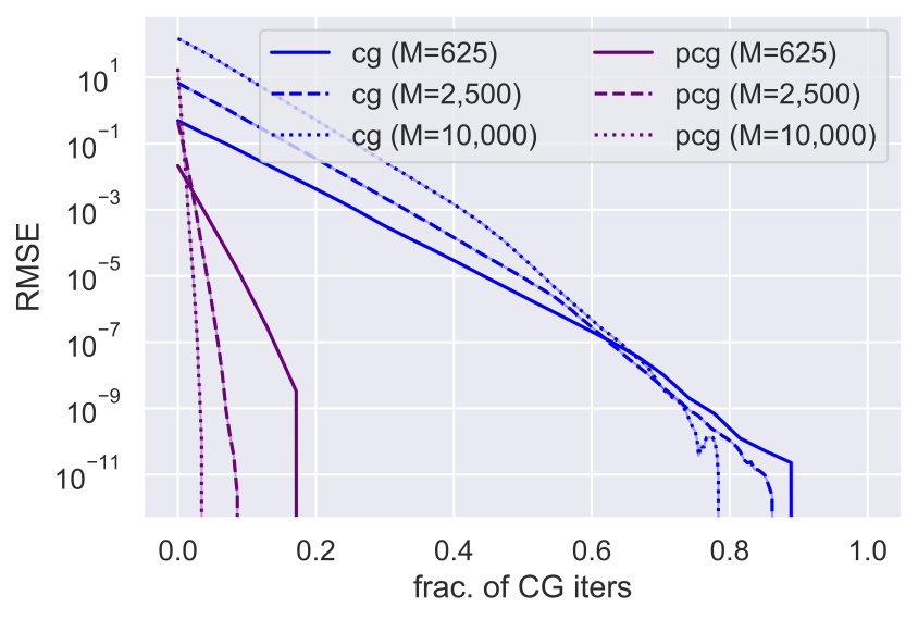
Figure 1: Convergence result of PCG v.s. CG. We compare PCG to standard CG for systems of size $M=625,2{,}500$ and $10{},000$ over 25 independent runs. We report RMSE as a function of the fraction of total CG iterations (to converge). PCG converges faster than CG, and for larger $M$ fewer iterations are required.

5.2 Speedup over Cholesky Decomposition

We examine the speedup of HIP-GP’s whitening strategy over the Cholesky whitening strategy in standard SVGP, by comparing the time for solving the correlation term $\boldsymbol{k}_{n}$. We generate 200 random 1D observations, and evenly-spaced inducing grids of size $M$ ranging from $10^{3}$ to $10^{6}$. We apply a set of kernels including the Matérn kernels with $\nu=0.5,1.5,2.5$ and the squared exponential kernel. The marginal variance is fixed to $0.1$ for all $M$. The length scale is set to $L/M$ where $L$ is the range of the data domain to utilize the inducing points efficiently. The PCG within the HIP-GP algorithm is run to convergence at tolerence 1e-10. The Cholesky decomposition is only available up to $M=10^{4}$ due to the memory limit. All experiments are run on a NVIDIA Tesla V100 GPU with 32GB memory.

We report the wall clock time of computations applied to Matérn ($2.5$) kernel in Tabel 1. The full report for all settings is presented in appendix. HIP-GP’s whitening strategy is consistently faster than the Cholesky whitening strategy across all experiments, and scales to larger $M$.

$M$	$10^{3}$	$10^{4}$	$10^{5}$	$10^{6}$
HIP-GP	$\mathbf{0.0045}$	$\mathbf{0.0185}$	$\mathbf{0.3475}$	$\mathbf{1.4595}$
SVGP	$0.0175$	$0.1745$	n/a	n/a

Table 1: Whitening time comparison (second) of HIP-GP v.s. SVGP with Matérn($2.5$) kernel.

5.3 Synthetic Derivative Observations

To validate our inter-domain SVGP framework, we study a derivative GP problem. We follow the work in Solak et al., (2003), which introduces derivative observations in addition to regular function observations to reduce uncertainty in learning dynamic systems. We synthesize a 1D GP function from a random neural network with sinusoidal non-linearities, and obtain function derivatives using automatic differentiation. The total observations consist of 100 function observations and 20 derivative observations, with added noise level $=0.05$ and $0.2$ respectively, as depicted in Figure 2(a).

We compare two inter-domain SVGP framework-based methods, HIP-GP and the standard SVGP, to the exact GP. We use the squared exponential kernel with signal variance $0.5$ and length scale $0.1$. For both HIP-GP and SVGP, we apply the full-rank variational family. The maximum number of PCG iterations within HIP-GP is set to 20. We evaluate the predictive performance on 100 test data. From Figure 2(b) and 2(c), we see that the inter-domain SVGP framework successfully utilizes the derivative observations to improve the prediction quality with reduced uncertainty, and is comparable to the exact method.

(a) Synthetic function and derivative observations

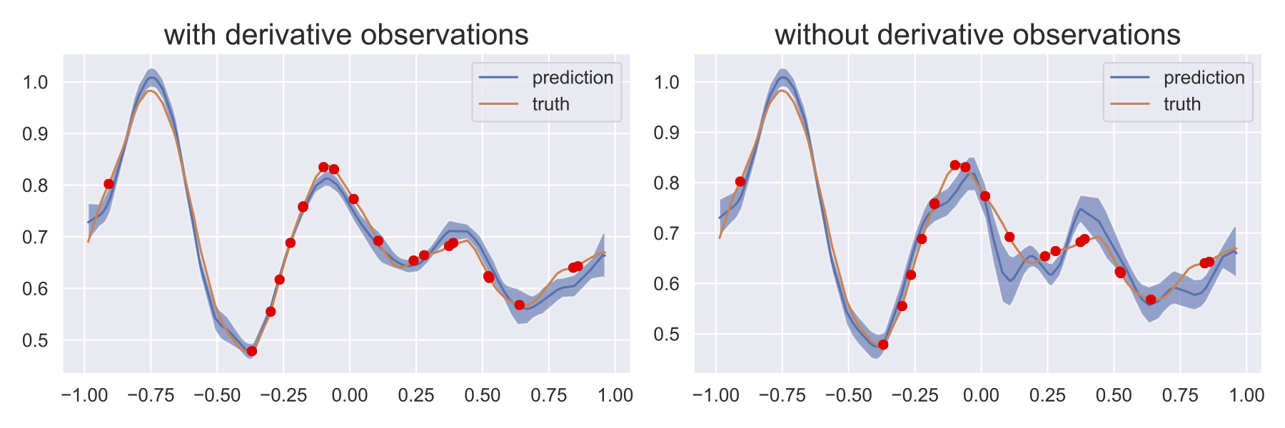
(b) HIP-GP posterior prediction with / without derivative observations for 100 test data. The solid blue line is the mean prediction and the shaded blue area is the 1 posterior standard deviation band. The red points indicate derivative observation locations with true function values.

	HIP-GP	SVGP	Exact GP
RMSE	0.0192	0.0192	0.0192
Uncertainty	0.0198	0.0206	0.0198

(c) Predictive RMSE and uncertainty (i.e. average standard deviation) for 100 test data.

Figure 2: GP with derivative observations analysis.

5.4 Spatial Analysis: UK Housing Prices

Now we test HIP-GP on a standard GP problem, i.e., the transformation $\mathcal{L}$ is an identity map. We apply HIP-GP to (log) prices of apartments as a function of latitude and longitude in England and Wales. The data include 180,947 prices from 2018, and we train on 160,947 observations and hold out 20,000 to report test error. We use the standard SVGP as baseline.

Scaling Inducing Points

We run HIP-GP on an increasingly dense grid of inducing points $M$. In all experiments, we use the Matérn ($2.5$) kernel and apply the block-independent variational family with neighboring block size $M_{b}=100~{}(10\times 10)$ for HIP-GP and SVGP. The maximum number of PCG iterations within HIP-GP is set to 20 and 50 for training and evaluation. The predictive performance measured by RMSE and the training time are displayed in Figure 3(c). From this result, we conclude that (i) increasing $M$ improves prediction quality; (ii) the performance of HIP-GP is almost indistinguishable to that of SVGP given the same $M$. (iii) Again, HIP-GP runs faster than SVGP and scales to larger $M$. The best prediction of HIP-GP is depicted in Figure 3(a) and 3(b).

(a) Posterior mean

(b) Posterior st. dev.

M	10,000	14,400	19,600	25,600	32,400	40,000
HIP-GP (RMSE)	0.411	0.409	0.400	0.397	0.393	0.389
SVGP (RMSE)	0.412	0.409	0.398	0.396	n/a	n/a
HIP-GP (time)	91.2	115.7	119.8	130.7	129.5	133.2
SVGP (time)	193.6	406.3	668.1	898.2	n/a	n/a

(c) Top row: predictive RMSE. Bottom row: average training time (second) per epoch.

Figure 3: UK Housing Analysis

PCG Iteration Early Stopping

Additionally, we examine the effect of the maximum number of PCG iterations when computing $\boldsymbol{k}_{n}$ on approximation quality. Figure 4 depicts test RMSE as a function of PCG iteration for $M=14{,}400$ on the test dataset of size $N=20{,}000$. The final approximation quality is robust to the number of PCG iterations used. The upshot is that HIP-GP needs only a small number of PCG iterations to be effective.

Figure 4: Stochastic optimization is robust to early stopping of PCG iterations.

5.5 Inferring Interstellar Dust Map

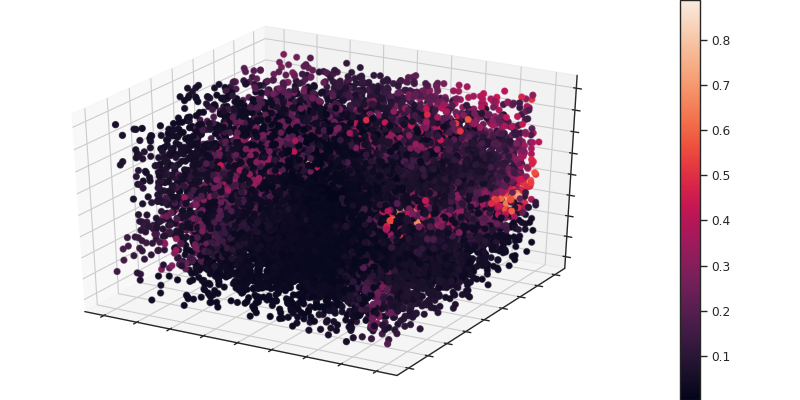
(a) Posterior mean of $\rho^{*}$

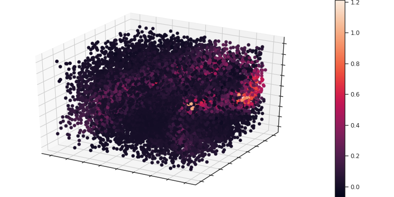
(b) Posterior mean of $\rho$

	MAE	MSE	loglike
HIP-GP ($M=62{,}500$)	0.0101	0.0012	2.3517
SVGP ($M=16{,}384$)	0.0153	0.0020	2.0690

(c) Predictive statistics for integrated observations

Figure 5: HIP-GP performance on 20,000 held-out data. Top: Posterior mean predictions in the integrated domain ($\rho^{*}$) and the latent domain ($\rho$). Bottom: We report the mean absolute error (MAE), the mean square error (MSE) and the test log likelihood in the intergrated domain.

Finally, we investigate an inter-domain GP problem with $\mathcal{L}$ being the integral transformation: inferring the interstellar dust map from integral observations. The interstellar dust map $\rho$ is a three-dimensional density function at each location in the Galaxy. The observations $y$, also known as the starlight extenctions, are noisy line integrals of the dust function (Rezaei Kh et al.,, 2017). We experiment with the Ananke dataset, which is comprised of $500{,}000$ starlight extinctions within $4\textrm{kpc}\times 4\textrm{kpc}\times 2\textrm{kpc}$ region of a high resolution Milky Way like galaxy simulation — a cutting edge simulation in the field because of the gas and dust resolution (Wetzel et al.,, 2016; Hopkins et al.,, 2018; Sanderson et al.,, 2020). Our goal is to infer the underlying dust map $\rho$ from the noisy extinctions $y$.

We compare HIP-GP with $M=62{,}500\,(50\times 50\times 25)$ and SVGP with $M=16{,}384\,(32\times 32\times 16)$ – the largest $M$ feasible. For both methods, we apply the block-independent variational parameterization with neighboring block size $M_{b}=8~{}(2\times 2\times 2)$, and the Matérn$\,(1.5)$ kernel. The maximum number of PCG iterations within HIP-GP is set to 200 and 500 for training and evaluation. We use Monte Carlo estimation to compute the inter-domain and transformed-domain covariance functions in Equations 7 and 8. We hold out 20,000 points for evaluation. The posterior mean predictions of the extinctions $\rho^{*}$ and the latent dust map $\rho$ are displayed in Figure 5(a) and 5(b). The predictive test statistics are summarized in Table 5(c). We see that with more inducing points, the predictive accuracy is enhanced. HIP-GP can scale to larger $M$ which enables better prediction quality, while SVGP is limited to $M$ around $16{,}000$.

6 DISCUSSION

We formulate a general SVGP framework for inter-domain GP problems. Upon this framework, we further scale the standard SVGP inference by developing the HIP-GP algorithm, with three technical innovations (i) a fast whitened parameterization, (ii) a novel preconditioner for fast linear system solves with hierarchical Toeplitz structure, and (iii) a structured variational approximation. The core idea of HIP-GP lies in the structured exploitations of the kernel matrix and the variational posterior. Therefore, it can be potentially extended to various settings, e.g. the case where a GP is a part of a bigger probabilistic model, and the non-Gaussian likelihoods thanks to recent advance in non-conjugate GP inference (Salimbeni et al.,, 2018).

Future works involve more in-depth analysis of such CG-based approximate GP methods. On the applied side, we will to apply HIP-GP to the Gaia dataset (Gaia et al.,, 2018) which consists of nearly 2 billion stellar observations.

 

Supplementary Materials: Hierarchical Inducing Point Gaussian Processes for Inter-domain Observations

 

Appendix A The HIP-GP Algorithm

We describe two algorithms that are core to the acceleration techniques we develop in Section 3.2. Algorithm 2 computes a fast MVM with a hierarchical Toeplitz matrix using the circulant embedding described in Algorithm 1. Note that we can similarly compute the MVM $\boldsymbol{R}^{\top}\boldsymbol{v}$ simply by adapting Algorithm 2 to perform FFT on $\boldsymbol{C}^{1/2}$ instead of on $\boldsymbol{C}$. Together these algorithms are sufficient for use within PCG to efficiently compute $\boldsymbol{k}_{n}$.

Data: $T$ ($N_{1}\times...\times N_{D}$ representation of hierarchical Toeplitz matrix);

Result: $C$ (circulant embedding of $T$)

$C\leftarrow T$ ;

  // copy

for $d\leftarrow 1$ to $D$ do

       $C_{r}\leftarrow\texttt{reverse-dim}(C,\text{dim}=d)$

       $C_{r}\leftarrow\texttt{chop-single-dim}(C_{r},\text{dim}=d)$

       $C_{r}\leftarrow\texttt{binary-zero-pad}(C_{r})$ ;

        // front pad

       $C\leftarrow\texttt{concat}(C,C_{r},\text{dim}=d)$

      

return $C$

Algorithm 1 Hierarchical circulant embedding.

Data: $\boldsymbol{k}_{0}$ (first row of $\boldsymbol{K}$ in $C$-order); $\boldsymbol{v}$ (vector, also in $C$-order); $N_{1},\dots,N_{D}$ (grid dimensions)

Result: $\boldsymbol{K}\boldsymbol{v}$ (matrix-vector product)

$T\leftarrow\texttt{reshape}(\boldsymbol{k}_{0},N_{1:D})$ ;

  // to $N_{1}\times\dots\times N_{D}$

$V\leftarrow\texttt{reshape}(\boldsymbol{v},N_{1:D})$ ;

  // to $N_{1}\times\dots\times N_{D}$

$C\leftarrow\texttt{Circ-Embed}(T,N_{1:D})$ ;

  //

$V\leftarrow\texttt{Zero-Embed}(V,N_{1:D})$ ;

  // match $C$

$res\leftarrow\texttt{ifft}(\texttt{fft}(C)\cdot\texttt{fft}(V))$ ;

  // $D$-dim fft

return flatten(res) ;

  // flatten in C-order

Algorithm 2 Matrix-vector multiplication $\boldsymbol{K}\boldsymbol{v}$ for a symmetric hierarchical Toeplitz matrix $\boldsymbol{K}$ and vector $\boldsymbol{v}$.

Appendix B Optimization Details

In this section, we derive the gradients for structured variational parameters and kernel hyperparameters.

B.1 Variational parameters

The structured variational posterior is characterized by $N(\boldsymbol{m},\boldsymbol{S})=\prod_{i=1}^{B}\mathcal{N}(\boldsymbol{m}_{i},\boldsymbol{S}_{i})$, where we decompose the $M\times M$ matrix $\boldsymbol{S}$ into $B$ block-independent covariance matrices of block size $M_{b}$:

$$\boldsymbol{S}=\begin{pmatrix}&\boldsymbol{S}_{1}\\ &&\boldsymbol{S}_{2}\\ &&&\cdots\\ &&&&\boldsymbol{S}_{B}\end{pmatrix},$$ (S1)

and the vector $\boldsymbol{m}$ into corresponding $B$ blocks: $\boldsymbol{m}_{1},\boldsymbol{m}_{2},\cdots,\boldsymbol{m}_{B}$.

B.1.1 Direct solves

We first consider directly solving the optimal $\boldsymbol{m}$ and $\boldsymbol{S}$.

Taking the derivatives of the HIP-GP objective w.r.t. $\boldsymbol{m}$ and $\boldsymbol{S}$, we obtain

$$\frac{\partial\mathcal{L}}{\partial\boldsymbol{S}_{i}} =-\frac{1}{2}\underbrace{\left((\sum_{n}\frac{1}{\sigma_{n}^{2}}\boldsymbol{k}_{n,i}\boldsymbol{k}_{n,i}^{\top})+\boldsymbol{I}_{M_{b}}\right)}_{\triangleq{\boldsymbol{\Lambda}}_{i}}+\frac{1}{2}\boldsymbol{S}_{i}^{-1}\,,\qquad\textrm{for }i=1:B$$ (S2)

$$\frac{\partial\mathcal{L}}{\partial\boldsymbol{m}} =\underbrace{\sum_{n}\frac{1}{\sigma_{n}^{2}}y_{n}\boldsymbol{k}_{n}}_{\triangleq\boldsymbol{b}}-\underbrace{\left(\sum_{n}\frac{1}{\sigma_{n}^{2}}\boldsymbol{k}_{n}\boldsymbol{k}_{n}^{\top}+\boldsymbol{I}_{M}\right)}_{\triangleq{\boldsymbol{\Lambda}}}\boldsymbol{m}$$ (S3)

where a vector or a matrix with subscript $i$, denotes its $i$-th block.

The optimum can be solved in closed form by setting the gradients equal to zero, i. e.

$$\frac{\partial\mathcal{L}}{\partial\boldsymbol{S}_{i}}=0\qquad\Rightarrow\qquad \boldsymbol{S}_{i}={\boldsymbol{\Lambda}}_{i}^{-1},\qquad\textrm{for }b=1:B$$ (S4)

$$\frac{\partial\mathcal{L}}{\partial\boldsymbol{m}}=0\qquad\Rightarrow\qquad \boldsymbol{m}={\boldsymbol{\Lambda}}^{-1}\boldsymbol{b}.$$ (S5)

If $M$ is very large, this direct solve will be infeasible. But note that ${\boldsymbol{\Lambda}}_{i},\boldsymbol{b}$ and ${\boldsymbol{\Lambda}}$ are all summations over some data terms, hence we can compute an unbiased gradient estimate using a small number of samples which is more efficient. We will use natural gradient descent (NGD) to perform optimization.

B.1.2 Natural gradient updates

To derive the NGD updates, we need the other two paramterizations of $N(\boldsymbol{m},\boldsymbol{S})$, namely,

• the canonical parameterization: $\{{\boldsymbol{\theta}}_{1,i}\}_{i=1}^{B},\{{\boldsymbol{\theta}}_{2,i}\}_{i=1}^{B}$ where ${\boldsymbol{\theta}}_{1,i}=\boldsymbol{S}_{i}^{-1}\boldsymbol{m}_{i}$ and ${\boldsymbol{\theta}}_{2,i}=-\frac{1}{2}\boldsymbol{S}_{i}^{-1}$, $i=1:B$; and

• the expectation parameterization: $\{\boldsymbol{\eta}_{1,i}\}_{i=1}^{B},\{\boldsymbol{\eta}_{2,i}\}_{i=1}^{B}$ where $\boldsymbol{\eta}_{1,i}=\boldsymbol{m}_{i}$ and $\boldsymbol{\eta}_{2,i}=\boldsymbol{m}_{i}\boldsymbol{m}_{i}^{\top}+\boldsymbol{S}_{i}$, $i=1:B$.

In Gaussian graphical models, the natural gradient for the canonical parameterization corresponds to the standard gradient for the expectation parameterization. That is,

$$\frac{\partial}{\partial\boldsymbol{\eta}}\mathcal{L} =\tilde{\nabla}_{{\boldsymbol{\theta}}}\mathcal{L},$$ (S6)

where $\tilde{\nabla}_{\theta}$ denotes the natural gradient w.r.t. $\theta$.

By the chain rule, we have

$$\frac{\partial\mathcal{L}}{\partial\boldsymbol{\eta}_{1,i}} =\frac{\partial\mathcal{L}}{\partial{\boldsymbol{m}_{i}}}\frac{\partial\boldsymbol{m}_{i}}{\partial\boldsymbol{\eta}_{1,i}}+\frac{\partial\mathcal{L}}{\partial\boldsymbol{S}_{i}}\frac{\partial\boldsymbol{S}_{i}}{\partial\boldsymbol{\eta}_{1,i}}$$ (S7)

$$=\boldsymbol{b}_{i}-\boldsymbol{S}_{i}^{-1}\boldsymbol{m}_{i}-[({\boldsymbol{\Lambda}}\boldsymbol{m})_{i}-{\boldsymbol{\Lambda}}_{i}\boldsymbol{m}_{i}],$$ (S8)

$$\frac{\partial\mathcal{L}}{\partial\boldsymbol{\eta}_{2,i}} =\frac{\partial\mathcal{L}}{\partial{\boldsymbol{m}_{i}}}\frac{\partial\boldsymbol{m}_{i}}{\partial\boldsymbol{\eta}_{2,i}}+\frac{\partial\mathcal{L}}{\partial\boldsymbol{S}_{i}}\frac{\partial\boldsymbol{S}_{i}}{\partial\boldsymbol{\eta}_{2,i}}$$ (S9)

$$=-\frac{1}{2}{\boldsymbol{\Lambda}}_{i}+\frac{1}{2}\boldsymbol{S}_{i}^{-1}.$$ (S10)

Therefore, the natural gradient updates for ${\boldsymbol{\theta}}$ are as follows:

$${\boldsymbol{\theta}}_{1,i} \leftarrow{\boldsymbol{\theta}}_{1,i}+l\frac{\partial\mathcal{L}}{\partial\boldsymbol{\eta}_{1,i}}={\boldsymbol{\theta}}_{1,i}+l\left(\boldsymbol{b}_{i}-\boldsymbol{S}_{i}^{-1}\boldsymbol{m}_{i}-[({\boldsymbol{\Lambda}}\boldsymbol{m})_{i}-{\boldsymbol{\Lambda}}_{i}\boldsymbol{m}_{i}]\right)$$ (S11)

$${\boldsymbol{\theta}}_{2,i} \leftarrow{\boldsymbol{\theta}}_{2,i}+l\frac{\partial\mathcal{L}}{\partial\boldsymbol{\eta}_{2,i}}={\boldsymbol{\theta}}_{2,i}+l\left(-\frac{1}{2}{\boldsymbol{\Lambda}}_{i}+\frac{1}{2}\boldsymbol{S}_{i}^{-1}\right),$$ (S12)

where $l$ is a positive step size.

B.2 Kernel hyperparameters

We now consider learning the kernel hyperparameters ${\boldsymbol{\theta}}$ with gradient descent.

For the convenience of notation, we denote the gram matrix $\boldsymbol{K}_{\boldsymbol{u},\boldsymbol{u}}$ as $\boldsymbol{K}$. HIP-GP computes $\boldsymbol{K}^{-1}\boldsymbol{v}$ by PCG. Directly auto-differentiating through PCG may be numerically instable. Therefore, we derive the analytical gradient for this part. Denote $\boldsymbol{c}$ as the first row of $\boldsymbol{K}$ — $\boldsymbol{c}$ fully characterizes the symmetric Toeplitz matrix $\boldsymbol{K}$. It suffices to manually compute the derivative w.r.t. $\boldsymbol{c}$, i.e. $\frac{\partial\boldsymbol{r}^{\top}\boldsymbol{K}^{-1}\boldsymbol{v}}{\partial\boldsymbol{c}}$, since by the following term $\frac{\partial\boldsymbol{c}}{\partial{\boldsymbol{\theta}}}$ can be taken care of with auto-differentiation.

We note the following equality

$$\frac{\partial\boldsymbol{r}^{\top}\boldsymbol{K}^{-1}\boldsymbol{v}}{\partial\boldsymbol{c}} =-(\boldsymbol{K}^{-1}\boldsymbol{r})^{\top}\frac{\partial\boldsymbol{K}}{\partial\boldsymbol{c}}\boldsymbol{K}^{-1}\boldsymbol{v}.$$ (S13)

The computation of $\boldsymbol{b}=\boldsymbol{K}^{-1}v$ is done in the forward pass and therefore can be cached for the backward pass. Additional computations in the backward pass are (1) $\boldsymbol{a}=\boldsymbol{K}^{-1}\boldsymbol{r}$ and (2) $\frac{\partial\boldsymbol{a}^{\top}\boldsymbol{K}\boldsymbol{b}}{\partial\boldsymbol{c}}$. (1) can be computed efficiently using the techniques developed in HIP-GP. Now we present the procedure to compute (2):

$$\frac{\partial\boldsymbol{a}^{\top}\boldsymbol{K}\boldsymbol{b}}{\partial\boldsymbol{c}} =\sum_{ij}a_{i}b_{j}\frac{\partial K_{ij}}{\partial\boldsymbol{c}}$$ (S14)

$$=\sum_{ij}a_{i}b_{j}\boldsymbol{e}_{|i-j|+1}$$ (S15)

$$=\textrm{toeplitz-mm}(b_{1}\boldsymbol{e}_{1},\boldsymbol{b},\boldsymbol{a})+\textrm{toeplitz-mm}(a_{1}\boldsymbol{e}_{1},\boldsymbol{a},\boldsymbol{b})-(\boldsymbol{a}^{\top}\boldsymbol{b})\boldsymbol{e}_{1},$$ (S16)

where $\boldsymbol{e}_{i}$ denotes the vector with a 1 in the $i$-th coordinate and 0’s elsewhere, and $\textrm{toeplitz-mm}(\boldsymbol{x},\boldsymbol{y},\boldsymbol{z})$ denotes the Toeplitz MVM $\boldsymbol{T}\boldsymbol{z}$, with the Toeplitz matrix $\boldsymbol{T}$ characterized by its first column vector $\boldsymbol{x}$ and first row vector $\boldsymbol{y}$ — this Toeplitz MVM can be also efficiently computed via its circulant embedding.

Appendix C Additional Experiment Results

C.1 Empirical analysis on preconditioner

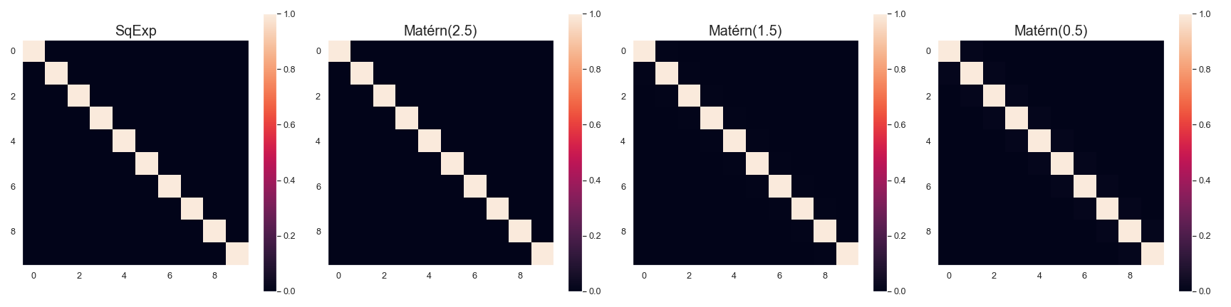
(a) Inducing point kernel matrix $\boldsymbol{K}_{\boldsymbol{u},\boldsymbol{u}}$ with $M=10$

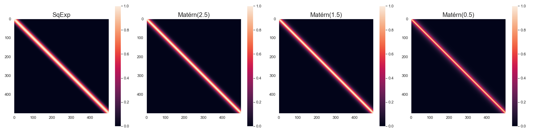
(b) Inducing point kernel matrix $\boldsymbol{K}_{\boldsymbol{u},\boldsymbol{u}}$ with $M=500$

(c) $r_{pcg}$ v.s. $M$ for different kernels.

Figure S1: Empirical analysis for preconditioner. The kernel lengthscale is 0.05.

In this section, we present an empirical analysis on the preconditioner developed in Section 3.2. Specifically, we investigate our intuition on the “banded property” that makes the preconditioner effective: when the number of inducing points $M$ is large enough, the inducing point Gram matrix $\boldsymbol{K}_{\boldsymbol{u},\boldsymbol{u}}$ is increasingly sparse, and therefore the upper left block of $\boldsymbol{C}^{-1}$ will be close to $\boldsymbol{K}_{\boldsymbol{u},\boldsymbol{u}}^{-1}$.

We note that the sparsity of the kernel matrix $\boldsymbol{K}_{\boldsymbol{u},\boldsymbol{u}}$ depends on three factors (1) $M$, the number of inducing points, (2) $l$, the lengthscale of the kernel, and (3) the property of the kernel function itself such as smoothness. To verify our intuition, we conduct the PCG convergence experiment by varying the combinations of these three factors. We evenly place $M$ inducing points in the $[0,2]$ interval that form the Gram matrix $\boldsymbol{K}_{\boldsymbol{u},\boldsymbol{u}}$, and randomly generate 25 vectors $\boldsymbol{v}$ of length $M$. We vary $M$ ranges from 10 to 500, and experiment with 4 types of kernel function: squared exponential kernel, Matérn (2.5), Matérn (1.5) and Matérn (0.5) kernels. For all kernels, we fix the signal variance $\sigma^{2}$ to 1 and the lengthscale $l$ to 0.05 and 0.5 in two separate settings. We run CG and PCG to solve $\boldsymbol{K}_{\boldsymbol{u},\boldsymbol{u}}^{-1}\boldsymbol{v}$ up to convergence with tolerance rate at 1e-10. We compare the fraction of # PCG iterations required for convergence over # CG iterations required for convergence, denoted as $r_{pcg}$. The results are displayed in Figure S1 (for $l=0.05$) and Figure S2 (for $l=0.5$).

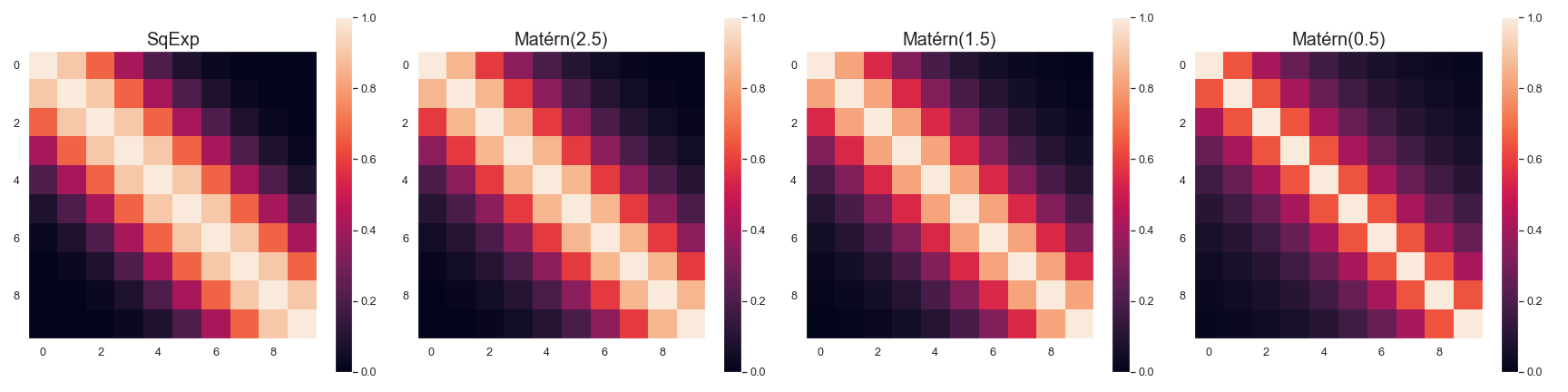
(a) Inducing point kernel matrix $\boldsymbol{K}_{\boldsymbol{u},\boldsymbol{u}}$ with $M=10$

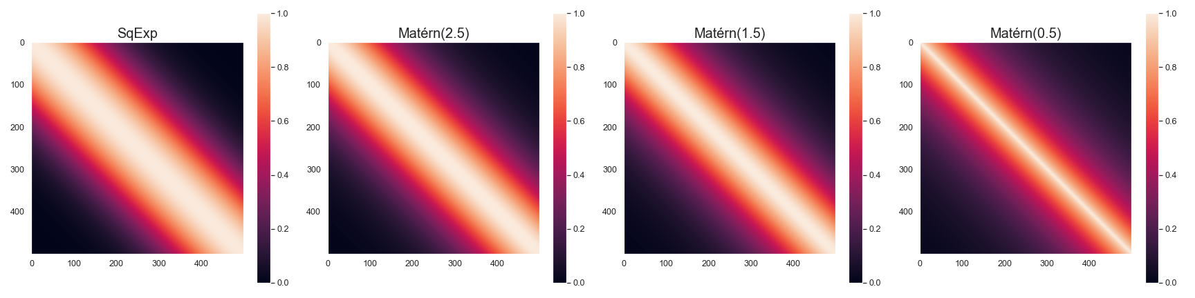
(b) Inducing point kernel matrix $\boldsymbol{K}_{\boldsymbol{u},\boldsymbol{u}}$ with $M=500$

(c) $r_{pcg}$ v.s. $M$ for different kernels.

Figure S2: Empirical analysis for preconditioner. The kernel lengthscale is 0.5.

Figure 1(a) - 1(b) and Figure 2(a) - 2(b) depict the kernel matrix $\boldsymbol{K}_{\boldsymbol{u},\boldsymbol{u}}$ for $M=10$ and $M=500$ with $l=0.05$ and $0.5$, respectively. Figure 1(c) and 2(c) plot $r_{pcg}$ over $M$ for different kernels and lengthscales. From these plots, we make the following observations:

1. $r_{pcg}$ are consistently smaller than 1, which verifies the effectiveness of the preconditioner.

2. In most cases, PCG converges faster when the system size $M$ is bigger. For example, $r_{pcg}$ decreases as $M$ increases in Figure 1(c) where $l=0.05$. However, we note that PCG convergence can be slowed down when the system size $M$ exceeds certain threshold in some cases (e.g.first three plots of Figure 2(c) where $l=0.5$). To see why this happens, we compare the plots of kernel matrices with $l=0.5$ for $M=10$ and $M=500$ in Figure 2(a) and 2(b). Since the lengthscale $l=0.5$ is relatively large with respect to the input domain range, the resulting $\boldsymbol{K}_{\boldsymbol{u},\boldsymbol{u}}$ for $M=10$ is sparse enough to approach a diagonal matrix. However, when we increase $M$ to 500, 1 lengthscale unit covers too many inducing points, making $\boldsymbol{K}_{\boldsymbol{u},\boldsymbol{u}}$ less “banded” and the preconditioner less effective. This observation is also consistent with our intuition.

3. For kernels that are less smooth, the PCG convergence speed-ups over CG are bigger given the same $M$, e.g. Matérn (0.5) kernel has smaller $r_{pcg}$ than squared exponential kernel does under the same configuration. We also observe that $\boldsymbol{K}_{\boldsymbol{u},\boldsymbol{u}}$ with Matérn (0.5) kernel is more diagonal-like than $\boldsymbol{K}_{\boldsymbol{u},\boldsymbol{u}}$ with squared exponential kernel from the kernel matrix plots. Together with (2), these results show that when the kernel matrix is more banded, the PCG convergence is accelerated more.

In conclusion, the PCG convergence speed depends on the “banded” property of the inducing point kernel matrix $\boldsymbol{K}_{\boldsymbol{u},\boldsymbol{u}}$, which further depends on $M$ and the smoothness of the kernel. As $\boldsymbol{K}_{\boldsymbol{u},\boldsymbol{u}}$ approaches a banded matrix, the preconditioner speeds up convergence drastically.

C.2 Additional experiment results for Section 5.2

We include additional experiment results on the other 3 kernels for Section 5.2, in Table S1- S3. These results are consistent to our conclusion in the paper.

$M$	$10^{3}$	$10^{4}$	$10^{5}$	$10^{6}$
HIP-GP	$\mathbf{0.0078}$	$\mathbf{0.0187}$	$\mathbf{0.3484}$	$\mathbf{1.4727}$
SVGP	$0.0152$	$0.1516$	n/a	n/a

Table S1: Whitening time comparison (second) of HIP-GP v.s. SVGP with Matérn($0.5$) kernel.

$M$	$10^{3}$	$10^{4}$	$10^{5}$	$10^{6}$
HIP-GP	$\mathbf{0.0087}$	$\mathbf{0.0192}$	$\mathbf{0.3479}$	$\mathbf{1.4656}$
SVGP	$0.0142$	$0.1379$	n/a	n/a

Table S2: Whitening time comparison (second) of HIP-GP v.s. SVGP with Matérn($1.5$) kernel.

$M$	$10^{3}$	$10^{4}$	$10^{5}$	$10^{6}$
HIP-GP	$\mathbf{0.0112}$	$\mathbf{0.0199}$	$\mathbf{0.3683}$	$\mathbf{2.3433}$
SVGP	$0.7090$	$0.0992$	n/a	n/a

Table S3: Whitening time comparison (second) of HIP-GP v.s. SVGP with squared exponential kernel.

C.3 UCI benchmark dataset

We include another experiment on the UCI 3D Road dataset ($N=278,319,D=3$). Following the same setup as Wang et al., 2019, we train HIP-GP with $M=36{,}000$ and a mean-field variational family, and compare to their reported results of Exact GP, SGPR ($M=512$) and SVGP ($M=1,024$) (Table S4). With the large $M$, HIP-GP achieves the smallest NLL, and the second-smallest RMSE (only beaten by exact GPs).

RMSE				NLL
HIP-GP	Exact GP	SGPR	SVGP	HIP-GP	Exact GP	SGPR	SVGP
$0.189$	$\mathbf{0.101}$	$0.661$	$0.481$	$\mathbf{-0.171}$	$0.909$	$0.943$	$0.697$

Table S4: UCI 3D Road experiment ($N=278{,}319$). Results are averaged over 3 random splits.

References

- Bauer et al., (2016) Bauer, M., van der Wilk, M., and Rasmussen, C. E. (2016). Understanding probabilistic sparse gaussian process approximations. In Advances in neural information processing systems, pages 1533–1541.
- Chan and Ng, (1996) Chan, R. H. and Ng, M. K. (1996). Conjugate gradient methods for toeplitz systems. SIAM review, 38(3):427–482.
- Cressie, (1990) Cressie, N. (1990). The origins of kriging. Mathematical Geology, 22(3):239–252.
- Cressie, (1992) Cressie, N. (1992). Statistics for spatial data. Terra Nova, 4(5):613–617.
- Cunningham et al., (2008) Cunningham, J. P., Shenoy, K. V., and Sahani, M. (2008). Fast gaussian process methods for point process intensity estimation. In International Conference on Machine Learning, pages 192–199. ACM.
- Cutajar et al., (2016) Cutajar, K., Osborne, M., Cunningham, J., and Filippone, M. (2016). Preconditioning kernel matrices. In International Conference on Machine Learning, pages 2529–2538.
- Dua and Graff, (2017) Dua, D. and Graff, C. (2017). UCI machine learning repository.
- Evans and Nair, (2018) Evans, T. W. and Nair, P. B. (2018). Scalable gaussian processes with grid-structured eigenfunctions (GP-GRIEF). In International Conference on Machine Learning.
- Gaia et al., (2018) Gaia, C., Brown, A., Vallenari, A., Prusti, T., de Bruijne, J., Babusiaux, C., Juhász, Á., Marschalkó, G., Marton, G., Molnár, L., et al. (2018). Gaia data release 2 summary of the contents and survey properties. Astronomy & Astrophysics, 616(1).
- Garnett et al., (2010) Garnett, R., Osborne, M. A., and Roberts, S. J. (2010). Bayesian optimization for sensor set selection. In Proceedings of the 9th ACM/IEEE international conference on information processing in sensor networks, pages 209–219.
- Green et al., (2015) Green, G. M., Schlafly, E. F., Finkbeiner, D. P., Rix, H.-W., Martin, N., Burgett, W., Draper, P. W., Flewelling, H., Hodapp, K., Kaiser, N., et al. (2015). A three-dimensional map of milky way dust. The Astrophysical Journal, 810(1):25.
- Hendriks et al., (2018) Hendriks, J. N., Jidling, C., Wills, A., and Schön, T. B. (2018). Evaluating the squared-exponential covariance function in gaussian processes with integral observations. arXiv preprint arXiv:1812.07319.
- Hensman et al., (2013) Hensman, J., Fusi, N., and Lawrence, N. D. (2013). Gaussian processes for big data. In Uncertainty in Artificial Intelligence, pages 282–290. AUAI Press.
- Hensman et al., (2015) Hensman, J., Matthews, A. G., Filippone, M., and Ghahramani, Z. (2015). MCMC for variationally sparse gaussian processes. In Advances in Neural Information Processing Systems, pages 1648–1656.
- Hestenes and Stiefel, (1952) Hestenes, M. R. and Stiefel, E. (1952). Methods of conjugate gradients for solving linear systems, volume 49. NBS Washington, DC.
- Hopkins et al., (2018) Hopkins, P. F., Wetzel, A., Kereš, D., Faucher-Giguère, C.-A., Quataert, E., Boylan-Kolchin, M., Murray, N., Hayward, C. C., Garrison-Kimmel, S., Hummels, C., et al. (2018). Fire-2 simulations: physics versus numerics in galaxy formation. Monthly Notices of the Royal Astronomical Society, 480(1):800–863.
- Izmailov et al., (2018) Izmailov, P., Novikov, A., and Kropotov, D. (2018). Scalable gaussian processes with billions of inducing inputs via tensor train decomposition. In Artificial Intelligence and Statistics, pages 726–735.
- Jidling et al., (2018) Jidling, C., Hendriks, J., Wahlström, N., Gregg, A., Schön, T. B., Wensrich, C., and Wills, A. (2018). Probabilistic modelling and reconstruction of strain. Nuclear Instruments and Methods in Physics Research Section B: Beam Interactions with Materials and Atoms, 436:141–155.
- Kh et al., (2017) Kh, S. R., Bailer-Jones, C., Hanson, R., and Fouesneau, M. (2017). Inferring the three-dimensional distribution of dust in the galaxy with a non-parametric method-preparing for gaia. Astronomy & Astrophysics, 598:A125.
- Lázaro-Gredilla and Figueiras-Vidal, (2009) Lázaro-Gredilla, M. and Figueiras-Vidal, A. (2009). Inter-domain gaussian processes for sparse inference using inducing features. In Advances in Neural Information Processing Systems, pages 1087–1095.
- Leike and Enßlin, (2019) Leike, R. and Enßlin, T. (2019). Charting nearby dust clouds using gaia data only. arXiv preprint arXiv:1901.05971.
- Minka, (2000) Minka, T. P. (2000). Deriving quadrature rules from gaussian processes. Technical report, Technical report, Statistics Department, Carnegie Mellon University.
- Murray and Adams, (2010) Murray, I. and Adams, R. P. (2010). Slice sampling covariance hyperparameters of latent gaussian models. In Advances in Neural Information Processing Systems, pages 1732–1740.
- Nocedal and Wright, (2006) Nocedal, J. and Wright, S. (2006). Numerical optimization. Springer Science & Business Media.
- Pleiss et al., (2020) Pleiss, G., Jankowiak, M., Eriksson, D., Damle, A., and Gardner, J. R. (2020). Fast matrix square roots with applications to gaussian processes and bayesian optimization. arXiv preprint arXiv:2006.11267.
- Rasmussen and Williams, (2006) Rasmussen, C. E. and Williams, C. K. I. (2006). Gaussian Processes for Machine Learning. The MIT Press.
- Rezaei Kh et al., (2017) Rezaei Kh, S., Bailer-Jones, C., Hanson, R., and Fouesneau, M. (2017). Inferring the three-dimensional distribution of dust in the galaxy with a non-parametric method. preparing for gaia. A&A, 598:A125.
- Riihimäki and Vehtari, (2010) Riihimäki, J. and Vehtari, A. (2010). Gaussian processes with monotonicity information. In Proceedings of the thirteenth international conference on artificial intelligence and statistics, pages 645–652. JMLR Workshop and Conference Proceedings.
- Saad, (2003) Saad, Y. (2003). Iterative methods for sparse linear systems. SIAM.
- Salimbeni et al., (2018) Salimbeni, H., Eleftheriadis, S., and Hensman, J. (2018). Natural gradients in practice: Non-conjugate variational inference in gaussian process models. arXiv preprint arXiv:1803.09151.
- Sanderson et al., (2020) Sanderson, R. E., Wetzel, A., Loebman, S., Sharma, S., Hopkins, P. F., Garrison-Kimmel, S., Faucher-Giguère, C.-A., Kereš, D., and Quataert, E. (2020). Synthetic gaia surveys from the fire cosmological simulations of milky way-mass galaxies. The Astrophysical Journal Supplement Series, 246(1):6.
- Shewchuk et al., (1994) Shewchuk, J. R. et al. (1994). An introduction to the conjugate gradient method without the agonizing pain.
- Shi et al., (2020) Shi, J., Titsias, M., and Mnih, A. (2020). Sparse orthogonal variational inference for gaussian processes. In International Conference on Artificial Intelligence and Statistics, pages 1932–1942. PMLR.
- Siivola et al., (2018) Siivola, E., Vehtari, A., Vanhatalo, J., González, J., and Andersen, M. R. (2018). Correcting boundary over-exploration deficiencies in bayesian optimization with virtual derivative sign observations. In 2018 IEEE 28th International Workshop on Machine Learning for Signal Processing (MLSP), pages 1–6. IEEE.
- Solak et al., (2003) Solak, E., Murray-Smith, R., Leithead, W. E., Leith, D. J., and Rasmussen, C. E. (2003). Derivative observations in gaussian process models of dynamic systems. In Advances in neural information processing systems, pages 1057–1064.
- Titsias, (2009) Titsias, M. (2009). Variational learning of inducing variables in sparse gaussian processes. In Artificial Intelligence and Statistics, pages 567–574.
- van der Wilk et al., (2020) van der Wilk, M., Dutordoir, V., John, S., Artemev, A., Adam, V., and Hensman, J. (2020). A framework for interdomain and multioutput gaussian processes. arXiv preprint arXiv:2003.01115.
- Wang et al., (2019) Wang, K. A., Pleiss, G., Gardner, J. R., Tyree, S., Weinberger, K. Q., and Wilson, A. G. (2019). Exact gaussian processes on a million data points. In Advances in Neural Information Processing Systems.
- Wetzel et al., (2016) Wetzel, A. R., Hopkins, P. F., Kim, J.-h., Faucher-Giguère, C.-A., Kereš, D., and Quataert, E. (2016). Reconciling dwarf galaxies with cdm cosmology: simulating a realistic population of satellites around a milky way–mass galaxy. The Astrophysical Journal Letters, 827(2):L23.
- Wills and Schön, (2017) Wills, A. G. and Schön, T. B. (2017). On the construction of probabilistic newton-type algorithms. In 2017 IEEE 56th Annual Conference on Decision and Control (CDC), pages 6499–6504. IEEE.
- Wilson and Nickisch, (2015) Wilson, A. and Nickisch, H. (2015). Kernel interpolation for scalable structured gaussian processes (kiss-gp). In International Conference on Machine Learning, pages 1775–1784.
- Wilson et al., (2015) Wilson, A. G., Dann, C., and Nickisch, H. (2015). Thoughts on massively scalable gaussian processes. arXiv preprint arXiv:1511.01870.
- Wilson et al., (2016) Wilson, A. G., Hu, Z., Salakhutdinov, R. R., and Xing, E. P. (2016). Stochastic variational deep kernel learning. In Advances in Neural Information Processing Systems, pages 2586–2594.