High-order linearly implicit structure-preserving exponential integrators for the nonlinear Schrödinger equation

Abstract

A novel class of high-order linearly implicit energy-preserving integrating factor Runge-Kutta methods are proposed for the nonlinear Schrödinger equation. Based on the idea of the scalar auxiliary variable approach, the original equation is first reformulated into an equivalent form which satisfies a quadratic energy. The spatial derivatives of the system are then approximated with the standard Fourier pseudo-spectral method. Subsequently, we apply the extrapolation technique/prediction- correction strategy to the nonlinear terms of the semi-discretized system and a linearized energy-conserving system is obtained. A fully discrete scheme is gained by further using the integrating factor Runge-Kutta method to the resulting system. We show that, under certain circumstances for the coefficients of a Runge-Kutta method, the proposed scheme can produce numerical solutions along which the modified energy is precisely conserved, as is the case with the analytical solution and is extremely efficient in the sense that only linear equations with constant coefficients need to be solved at every time step. Numerical results are addressed to demonstrate the remarkable superiority of the proposed schemes in comparison with other existing structure-preserving schemes.
AMS subject classification: 65M06, 65M70
Keywords: SAV approach, energy-preserving, integrating factor Runge-Kutta method, linearly implicit, nonlinear Schrödinger equation.

1 Introduction

We consider the nonlinear Schrödinger equation (NLSE) given as follows:

$$\left\{\begin{aligned} &\text{i}\partial_{t}\phi({\bf x},t)+\mathcal{L}\phi({\bf x},t)+\beta|\phi({\bf x},t)|^{2}\phi({\bf x},t)=0,\ ({\bf x},t)\in\Omega,\ t>0,\\ &\phi({\bf x},0)=\phi_{0}({\bf x}),\ {\bf x}\in\Omega\subset\mathbb{R}^{d},\ d=1,2,3,\end{aligned}\right.$$ (1.1)

where $t$ is the time variable, ${\bf x}$ is the spatial variable, $\text{i}=\sqrt{-1}$ is the complex unit, $\phi:=\phi({\bf x},t)$ is the complex-valued wave function, $\mathcal{L}$ is the usual Laplace operator, $\beta$ is a given real constant, and $\phi_{0}({\bf x})$ is a given initial data. The nonlinear Schrödinger equation (1.1) satisfies the following two invariants, that is mass

$$\mathcal{M}(t)=\int_{\Omega}|\phi|^{2}d{\bf x}\equiv\mathcal{M}(0),\ t\geq 0,$$ (1.2)

and Hamiltonian energy

$$\mathcal{E}(t)=\int_{\Omega}\Big{(}-|\nabla\phi|^{2}+\frac{\beta}{2}|\phi|^{4}\Big{)}d{\bf x}\equiv\mathcal{E}(0),\ t\geq 0.$$ (1.3)

A numerical scheme that preserves one or more invariants of the original systems is called an energy-preserving method or integral-preserving method. The earlier attempts to develop energy-preserving methods for NLSE can date back to 1981, when Delfour, Fortin, and Payre [22] constructed a two-level finite difference scheme (also called Crank-Nicolson finite difference (CNFD) scheme) which can satisfy the discrete analogue of conservation laws (1.2) and (1.3). Some comparisons with nonconservation schemes are investigated by Sanz-Serna and Verwer [50], which show the nonconservative schemes may easily show nonlinear blow-up. Furthermore, it can be proven rigorously in mathematics that the CNFD scheme is second-order accurate in time and space [6, 7, 56]. Up to now, the energy-preserving Crank-Nicolson schemes for NLSE are extensively extended and analyzed [2, 3, 17, 24, 27, 42, 58]. Furthermore, we note that the discrete conservative laws play a crucial role in numerical analyses for numerical schemes of NLSE. However, it is fully implicit and at every time step, a nonlinear equation shall be solved by using a nonlinear iterative method and thus it may be time consuming. Other fully implicit energy-preserving schemes for NLSE provided by the averaged vector flied method [48] and the discrete variational derivative method [21, 25] can be founded in [16, 26, 39, 46]. Zhang et al. [60] firstly proposed a linearly implicit Crank-Nicolson finite difference (LI-CNFD) scheme in which a linear system is to be solved at every time step. Thus it is computationally much cheaper than that of the CNFD scheme. The LI-CNFD scheme can satisfy a new discrete analogue of conservation laws (1.2) and (1.3) and its stability and convergence is analyzed in [56]. Another popular linearly implicit energy-preserving method is the relaxation finite difference scheme [9]. More recently, the scalar auxiliary variable (SAV) approach [53, 54] have been a particular powerful tool for the design of linearly implicit energy-preserving numerical schemes for NLSE [5]. Nevertheless, to our best knowledge, all of the schemes can achieve at most second-order in time, which cannot provide long time accurate solutions for a given large time step.

It has been proven that no Runge-Kutta (RK) method can preserve arbitrary polynomial invariants of degree 3 or higher of arbitrary vector fields [14]. Thus, over that last decades, how to develop high-order energy-preserving methods for general conservation systems attracts a lot of attention. The notable ones include, but are not limited to, high-order averaged vector field (AVF) methods [45, 48], Hamiltonian Boundary Value Methods (HBVMs) [11, 12] and energy-preserving continuous stage Runge-Kutta methods (CSRKs) [19, 30, 47, 57]. Actually, the HBVMs and CSRKs have been shown to be an efficient method to develop high-order energy-preserving schemes for NLSE [8, 44], however, the proposed schemes are fully implicit. At every time step, one needs to solve a large fully nonlinear system and thus it might be lead to high computational costs.

Due to the high computational cost of the high-order fully implicit schemes, in the literatures, ones are devoted to construct energy-preserving explicit schemes for NLSE. Based on the invariant energy quadratization (IEQ) approach [59] or the SAV approach and the projection method [13, 31, 29], the authors proposed some explicit energy-preserving schemes for NLSE [35, 61]. Such scheme is extremely easy to implement, however, it is conditionally stable so that it may require very small time step sizes due to the certain time step restriction. Especially, this restriction is more serious in 2D and 3D. Compared with the fully explicit scheme, the linearly implicit scheme is unconditionally stable so that the time step restriction can be removed. Furthermore, the linearly implicit scheme only need to solve a linear system of equations at every time step, thus it is more efficient than the fully implicit scheme. In light of this, Li et al. proposed a class of linearly implicit schemes for NLSE, which can preserve the discrete analogue of conservation law (1.2) [43]. It involves solving linear equations with complicated variable coefficients at every time step and thus it is may be very time consuming. Another way to achieve this goal is to combine the SAV approach with the extrapolation technique or the prediction-correction strategy [10]. However, at every time step, the constant coefficient matrix of the scheme may admit a large norm arising from a space discretization of the linear unbounded differential operator $\mathcal{L}$ [15].

It is well-known that the exponential integrator often involve exact integration of the linear part of the target equation, and thus it can achieve high accuracy, stability for a very stiff differential equation, such as highly oscillatory ODEs and semidiscrete time-dependent PDEs. For more details on the exponential integrator, please refer to the excellent review article provided by Hochbruck and Ostermann [33]. As a matter of fact, many energy-preserving exponential integrators have been done for the conservative systems in the past few decades. Based on the projection approach, Celledoni et al. developed some symmetry- and energy-preserving implicit exponential schemes for the cubic Schrödinger equation [15]. By combining the exponential integrator with the AVF method, Li and Wu constructed a class of second-order implicit energy-preserving exponential schemes for canonical Hamiltonian systems and successfully applied it to solve NLES [45]. Further analysis and generalization is investigated by Shen and Leok [55]. More recently, Jiang et al. showed that the SAV approach is also an efficient approach to develop second-order linearly implicit energy-preserving exponential integrator for NLSE [34]. Overall, there exist very few works devoted to development of high-order linearly implicit energy-preserving exponential schemes for NLSE, which motivates this paper. We should note that, in general, the particularly interesting types of exponential integrators are integrating factor (IF) methods and exponential time differencing (ETD) methods, respectively and we here mainly focus on the high-order linearly implicit energy-preserving IF schemes.

In this paper, following the idea of the SAV approach, we firstly reformulate the original system (1.1) into a new system by introducing a new auxiliary variable, which satisfies a modified energy. The spatial discretization is then performed with the standard Fourier pseudo-spectral method [18, 51]. Subsequently, the extrapolation technique/ prediction-correction strategy is employed to the nonlinear terms of the semi-discrete system and a linearized energy-conserving system is obtained. Based on the Lawson transformation, the semi-discrete system is rewritten as an equivalent form and the fully discrete scheme is obtained by using a RK method to the linearized equation. We show that, the proposed scheme can preserve the modified energy in the discretized level when some under certain circumstances are imposed on the coefficients of the Runge-Kutta method and at every time step, only a linear equations with constant coefficients is solved in which there is no existing references [10, 41] considering this issue.

The rest of this paper is organized as follows. In Section 2, we use the idea of the SAV approach to reformulate the original equation (1.1) into a new reformulation, which satisfies a modified energy. In Section 3, two class of linearly implicit energy-preserving integrating factor Runge-Kutta methods are proposed for NLSE (1.1). In Section 4, several numerical examples are investigated to illustrate the efficiency of the proposed scheme. We draw some conclusions in Section 5.

2 Model reformulation

In this section, we first employ the SAV approach to reformulate the NLSE (1.1) into a new reformulation which satisfies a quadratic energy. The resulting reformulation provides an elegant platform for developing high-order linearly implicit energy-preserving schemes.

Based on the idea of the SAV approach [53, 54], we introduce an auxiliary variable

$$p:=p(t)=\sqrt{(\phi^{2},\phi^{2})+C_{0}},$$

where $C_{0}\geq 0$ is a constant to make $p$ well-defined for all $\phi$. Here, $(v,w)$ is the continuous inner product defined by $\int_{\Omega}v\bar{w}d{\bf x}$ where $\bar{w}$ represents the conjugate of $w$. Then, the Hamiltonian energy functional is rewritten as the following quadratic form

$$\mathcal{E}(t)=({\mathcal{L}}\phi,\phi)+\frac{\beta}{2}p^{2}-\frac{\beta}{2}C_{0}.$$

According to the energy variational principle, we obtain the following SAV reformulated system

$$\left\{\begin{aligned} &\partial_{t}\phi=\text{i}\bigg{(}{\mathcal{L}}\phi+\frac{\beta|\phi|^{2}\phi p}{\sqrt{(\phi^{2},\phi^{2})+C_{0}}}\bigg{)},\\ &\frac{d}{dt}p=2{\rm Re}\bigg{(}\text{i}{\mathcal{L}}\phi,\frac{|\phi|^{2}\phi}{\sqrt{(\phi^{2},\phi^{2})+C_{0}}}\bigg{)},\end{aligned}\right.$$ (2.1)

with the consistent initial condition

$$\phi({\bf x},0)=\phi_{0}({\bf x}),\ p(0)=\sqrt{\big{(}\phi^{2}_{0}({\bf x}),\phi^{2}_{0}({\bf x}))+C_{0}},$$ (2.2)

where ${\rm Re}(u)$ represents the real part of $u$.

Theorem 2.1.

The SAV reformulation (2.1) preserves the following quadratic energy

$$\frac{d}{dt}\mathcal{E}(t)=0,\ \mathcal{E}(t)=(\mathcal{L}\phi,\phi)+\frac{\beta}{2}p^{2}-\frac{\beta}{2}C_{0},\ t\geq 0.$$ (2.3)

Proof.

It is clear to see

$$\frac{d}{dt}\mathcal{E}(t) =2\text{Re}(\mathcal{L}\phi,\partial_{t}\phi)+\beta p\partial_{t}p$$

$$=2\beta p\text{Re}\Big{(}\mathcal{L}\phi,\text{\rm i}\frac{|\phi|^{2}\phi}{\sqrt{(\phi^{2},\phi^{2})+C_{0}}}\Big{)}+\beta p\partial_{t}p$$

$$=-\beta p\partial_{t}p+\beta p\partial_{t}p$$

$$=0.$$

This completes the proof. ∎

3 The construction of the high-order linearly integrating factor Runge-Kutta methods

In this section, a class of high-order linearly implicit energy-preserving integrating factor Runge-Kutta methods are proposed for the SAV reformulated system (2.1). For simplicity, in this paper, we shall introduce our schemes in two space dimension, i.e., $d=2$ in (2.1). Generalizations to $d=1$ or $3$ are straightforward.

3.1 Spatial discretization

We set the computational domain $\Omega=[a,b]\times[c,d]$ and let $l_{x}=b-a$ and $l_{y}=d-c$. Choose the mesh sizes $h_{x}=l_{x}/N_{x}$ and $h_{y}=l_{y}/N_{y}$ with two even positive integers $N_{x}$ and $N_{y}$, and denote the grid points by $x_{j}=jh_{x}$ for $j=0,1,2,\cdots,N_{x}$ and $y_{k}=kh_{y}$ for $k=0,1,2,\cdots,N_{y}$; let $\phi_{j,k}$ be the numerical approximation of $\phi(x_{j},y_{k},t)$ for $j=0,1,\cdots,N_{x},k=0,1,2,\cdots,N_{y}$, and

$$\phi:=(\phi_{0,0},\phi_{1,0},\cdots,\phi_{N_{x}-1,0},\phi_{0,1},\phi_{1,1},\cdots,\phi_{N_{x}-1,1},\cdots,\phi_{0,N_{y}-1},\phi_{1,N_{y}-1},\cdots,\phi_{N_{x}-1,N_{y}-1})^{T}$$

be the solution vector; we also define the discrete inner product, $L^{2}$-norm and $L^{\infty}$-norm as, respectively,

$$\langle\phi,\psi\rangle_{h}=h_{x}h_{y}\sum_{j=0}^{N_{x}-1}\sum_{k=0}^{N_{y}-1}\phi_{j,k}\bar{\psi}_{j,k},\ \|\phi\|_{h}^{2}=\langle\phi,\phi\rangle_{h},\ \|{\phi}\|_{h,\infty}=\max\limits_{j,k}|\phi_{j,k}|.$$

In addition, we denote $`\cdot$’ as the element product of vectors ${\phi}$ and ${\psi}$, that is

$$\phi\cdot\psi= \big{(}\phi_{0,0}\psi_{0,0},\cdots,\phi_{N_{x}-1,0}\psi_{N_{x}-1,0},\cdots,\phi_{0,N_{x}-1}\psi_{0,N_{y}-1},\cdots,\phi_{N_{x}-1,N_{y}-1}\psi_{N_{x}-1,N_{y}-1}\big{)}^{T}.$$

For brevity, we denote ${\phi}\cdot\phi$ and ${\phi}\cdot\bar{\phi}$ as ${\phi}^{2}$ and $|\phi|^{2}$, respectively.

Denote the interpolation space as

$$\mathcal{T}_{h}=\text{span}\{g_{j}(x)g_{k}(y),\ 0\leq j\leq N_{x}-1,0\leq k\leq N_{y}-1\}$$

where $g_{j}(x)$ and $g_{k}(y)$ are trigonometric polynomials of degree $N_{x}/2$ and $N_{y}/2$, given, respectively, by

$$g_{j}(x)=\frac{1}{N_{x}}\sum_{l=-N_{x}/2}^{N_{x}/2}\frac{1}{a_{l}}e^{\text{i}l\mu_{x}(x-x_{j})},\ g_{k}(y)=\frac{1}{N_{y}}\sum_{l=-N_{y}/2}^{N_{y}/2}\frac{1}{b_{l}}e^{\text{i}l\mu_{y}(y-y_{k})},$$

with $a_{l}=\left\{\begin{aligned} &1,\ |l|<\frac{N_{x}}{2},\\ &2,\ |l|=\frac{N_{x}}{2},\end{aligned}\right.,\ b_{l}=\left\{\begin{aligned} &1,\ |l|<\frac{N_{y}}{2},\\ &2,\ |l|=\frac{N_{y}}{2},\end{aligned}\right.$, $\mu_{x}=\frac{2\pi}{l_{x}}$ and $\mu_{y}=\frac{2\pi}{l_{y}}$. We then define the interpolation operator $I_{N}:C(\Omega)\to\mathcal{T}_{h}$ as:

$$I_{N}\phi(x,y,t)=\sum_{j=0}^{N_{x}-1}\sum_{k=0}^{N_{y}-1}\phi_{j,k}(t)g_{j}(x)g_{k}(y),$$

where $\phi_{j,k}(t)=\phi(x_{j},y_{k},t)$.

Taking the derivative with respect to $x$ and $y$, respectively, and then evaluating the resulting expressions at the collocation points ($x_{j},y_{k}$), we have

$$\frac{\partial^{2}I_{N}\phi(x_{j},y_{k},t)}{\partial x^{2}} =\sum_{l=0}^{N_{x}-1}\phi_{l,k}(t)\frac{d^{2}g_{l}(x_{j})}{dx^{2}}=\sum_{l=0}^{N_{x}-1}(D_{2}^{x})_{j,l}\phi_{l,k}(t),$$ (3.1)

$$\frac{\partial^{2}I_{N}\phi(x_{j},y_{k},t)}{\partial y^{2}} =\sum_{l=0}^{N_{y}-1}\phi_{j,l}\frac{d^{2}g_{l}(y_{k})}{dy^{2}}=\sum_{l=0}^{N_{y}-1}\phi_{j,l}(t)(D_{2}^{y})_{k,l},$$ (3.2)

where

$$(D^{x}_{2})_{j,k}=\left\{\begin{aligned} &\frac{1}{2}\mu_{x}^{2}(-1)^{j+k+1}\csc^{2}(\mu_{x}\frac{x_{j}-x_{k}}{2}),\ &j\neq k,\\ &-\mu_{x}^{2}\frac{N_{x}^{2}+2}{12},\quad\quad\quad\quad~{}&j=k,\end{aligned}\right.$$

$$(D^{y}_{2})_{j,k}=\left\{\begin{aligned} &\frac{1}{2}\mu_{y}^{2}(-1)^{j+k+1}\csc^{2}(\mu_{y}\frac{y_{j}-y_{k}}{2}),\ &j\neq k,\\ &-\mu_{y}^{2}\frac{N_{y}^{2}+2}{12},\quad\quad\quad\quad~{}&j=k.\end{aligned}\right.$$

Remark 3.1.

We should note that [51]

$$D_{2}^{w}=\mathcal{F}_{w}^{H}\Lambda_{w}\mathcal{F}_{w},\ w=x,y,$$

where

$$\Lambda_{w}=\Big{(}\text{\rm i}\frac{2\pi}{l_{w}}\Big{)}^{2}\text{\rm diag}\Big{[}0,1,\cdots,\frac{N_{w}}{2},-\frac{N_{w}}{2}+1,\cdots,-2,-1\Big{]}^{2},$$

and $\mathcal{F}_{w}$ is the discrete Fourier transform (DFT) and $\mathcal{F}_{w}^{H}$ represents the conjugate transpose of $\mathcal{F}_{w}$.

Then, we use the standard Fourier pseudo-spectral method to solve (2.1) and obtain

$$\left\{\begin{aligned} &\frac{d}{dt}\phi=\text{i}\bigg{(}{\mathcal{L}}_{h}\phi+\frac{\beta|\phi|^{2}\cdot\phi p}{\sqrt{\langle\phi^{2},\phi^{2}\rangle_{h}+C_{0}}}\bigg{)},\\ &\frac{d}{dt}p=2{\rm Re}\bigg{\langle}\text{i}{\mathcal{L}}_{h}\phi,\frac{|\phi|^{2}\cdot\phi}{\sqrt{\langle\phi^{2},\phi^{2}\rangle_{h}+C_{0}}}\bigg{\rangle}_{h},\end{aligned}\right.$$ (3.3)

where ${\mathcal{L}}_{h}=I_{N_{y}}\otimes D_{2}^{x}+D_{2}^{y}\otimes I_{N_{x}}$ is the spectral differentiation matrix and $\otimes$ represents the Kronecker product.

Theorem 3.1.

The semi-discrete system (3.3) preserves the following semi-discrete quadratic energy

$$\frac{d}{dt}E_{h}(t)=0,\ E_{h}(t)=\langle\mathcal{L}_{h}\phi,\phi\rangle_{h}+\frac{\beta}{2}p^{2}-\frac{\beta}{2}C_{0},\ t\geq 0.$$ (3.4)

Proof.

The proof is similar to Theorem 2.1, thus, for brevity, we omit it.

3.2 Temporal exponential integration

Denote $t_{n}=n\tau,$ and $t_{ni}=t_{n}+c_{i}\tau,\ i=1,2,\cdots,s$, $n=0,1,2,\cdots,$ where $\tau$ is the time step and $c_{1},c_{2},\cdots,c_{s}$ are distinct real numerbers (usually $0\leq c_{i}\leq 1$). The approximations of the function $\phi(x,y,t)$ at points $(x_{j},y_{k},t_{n})$ and $(x_{j},y_{k},t_{ni})$ are denoted by $\phi_{j,k}^{n}$ and $(\phi_{ni})_{j,k}$, and the approximations of the function $p(t)$ at points $t_{n}$ and $t_{ni}$ are denoted by $p^{n}$ and $p_{ni}$.

3.2.1 Linearly implicit integrating factor Runge-Kutta method based on the extrapolation method

We assume that the numerical solutions of $\phi$ for (3.3) from $t=0$ to $t\leq t_{n}$ are obtained. Then we obtain the Lagrange interpolating polynomial (denoted by $\mathcal{P}(t)$) based on the time nodes $t_{k},\ t_{k}+c_{i}\tau,$ and the values $\phi^{k},\ \phi_{ki}$, where $\ 0\leq k\leq n,\ i=1,2,\cdots,s$. Subsequently, we use $\mathcal{P}(t)$ to approximate $\phi$ of the nonlinear terms of (3.3) over time interval $(t_{n},t_{n+1}]$ and a linearized system is obtained, as follows:

$$\left\{\begin{aligned} &\frac{d}{dt}\tilde{\phi}=\text{i}\bigg{(}{\mathcal{L}}_{h}\tilde{\phi}+\frac{\beta|\mathcal{P}(t)|^{2}\cdot\mathcal{P}(t)\tilde{p}}{\sqrt{\langle\mathcal{P}(t)^{2},\mathcal{P}(t)^{2}\rangle_{h}+C_{0}}}\bigg{)},\\ &\frac{d}{dt}\tilde{p}=2{\rm Re}\bigg{\langle}\text{i}{\mathcal{L}}_{h}\tilde{\phi},\frac{|\mathcal{P}(t)|^{2}\cdot\mathcal{P}(t)}{\sqrt{\langle\mathcal{P}(t)^{2},\mathcal{P}(t)^{2}\rangle_{h}+C_{0}}}\bigg{\rangle}_{h},\ t\in(t_{n},t_{n+1}],\end{aligned}\right.$$ (3.5)

where $n=0,1,2,\cdots,$ $\tilde{\phi}:=\tilde{\phi}(t)$ and $\tilde{p}:=\tilde{p}(t)$ are approximations of $\phi(t)$ and $p(t)$, respectively over time interval $(t_{n},t_{n+1}],\ n=0,1,2,\cdots,$.

Remark 3.2.

It is remarked that, by the similar argument as Theorem 2.1, we can show the linearized system (3.5) satisfies a semi-discrete quadratic energy, as follows:

$$\frac{d}{dt}\tilde{E}_{h}(t)=0,\ \tilde{E}_{h}(t)=\langle\mathcal{L}_{h}\tilde{\phi},\tilde{\phi}\rangle_{h}+\frac{\beta}{2}(\tilde{p})^{2}-\frac{\beta}{2}C_{0},\ t\geq 0.$$

By using the Lawson transformation [40], we multiply both sides of the first equation of (3.5) by the operator $\rm exp(-{\rm i}{\mathcal{L}}_{h}t)$, and then introduce $\Psi=\rm exp(-{\rm i}{\mathcal{L}}_{h}t){\color[rgb]{0,0,1}\tilde{\phi}}$ to transform (3.5) into an equivalent form, as follows:

$$\left\{\begin{aligned} &\frac{d}{dt}\Psi={\rm i}\exp(-{\rm i}\mathcal{L}_{h}t)\frac{\beta|\mathcal{P}(t)|^{2}\cdot\mathcal{P}(t){\color[rgb]{0,0,1}\tilde{p}}}{\sqrt{\langle\mathcal{P}(t)^{2},\mathcal{P}(t)^{2}\rangle_{h}+C_{0}}},\\ &\frac{d}{dt}{\color[rgb]{0,0,1}\tilde{p}}=\!2{\rm Re}\Bigg{\langle}\!\!{\rm i}\exp({\rm i}\mathcal{L}_{h}t){\mathcal{L}}_{h}\Psi,\frac{|\mathcal{P}(t)|^{2}\cdot\mathcal{P}(t)}{\sqrt{\big{\langle}\mathcal{P}(t)^{2},\mathcal{P}(t)^{2}\big{\rangle}_{h}+C_{0}}}\Bigg{\rangle}_{h},\ t\in(t_{n},t_{n+1}],\end{aligned}\right.$$ (3.6)

where $n=0,1,2,\cdots,$.

We first apply an RK method to the linearized system (3.6), and then the discretization is rewritten in terms of the original variables to give a class of linearly implicit integrating factor Runge-Kutta methods (LI-IF-RKMs), as follows:

Scheme 3.1.

Let $b_{i},a_{ij}\ (i,j=1,\cdots,s)$ be real numbers and let $c_{i}=\sum_{j=1}^{s}a_{ij}$. For given $\phi^{n}$, $p^{n}$ and $\phi_{ni}^{*}=\mathcal{P}(t_{n}+c_{i}\tau),i=1,\cdots,s$, $s$-stage linearly implicit integrating factor Runge-Kutta method is given by

$$\left\{\begin{aligned} &\phi_{ni}=\exp({\rm i}\mathcal{L}_{h}c_{i}\tau)\phi^{n}+\tau\sum_{j=1}^{s}a_{ij}\exp({\rm i}\mathcal{L}_{h}(c_{i}-c_{j})\tau)k_{j},\\ &p_{ni}=p^{n}+\tau\sum_{j=1}^{s}a_{ij}l_{j},\ l_{i}\!=2{\rm Re}\!\Big{\langle}\!{\rm i}\mathcal{L}_{h}\phi_{ni},\frac{|\phi_{ni}^{*}|^{2}\cdot\phi_{ni}^{*}}{\sqrt{\big{\langle}(\phi_{ni}^{*})^{2},(\phi_{ni}^{*})^{2}\big{\rangle}_{h}\!+\!C_{0}}}\Big{\rangle}_{h},\\ &k_{i}\!=\!{\rm i}\ \frac{\beta|\phi_{ni}^{*}|^{2}\cdot\phi_{ni}^{*}p_{ni}}{\sqrt{\big{\langle}(\phi_{ni}^{*})^{2},(\phi_{ni}^{*})^{2}\big{\rangle}_{h}\!+\!C_{0}}},\end{aligned}\right.$$ (3.7)

where $i=1,2,\cdots,s$. Then $(\phi^{n+1},p^{n+1})$ are updated by

$$\left\{\begin{aligned} &\phi^{n+1}=\exp({\rm i}\mathcal{L}_{h}\tau)\phi^{n}+\tau\sum_{i=1}^{s}b_{i}\exp({\rm i}\mathcal{L}_{h}(1-c_{i})\tau)k_{i},\\ &p^{n+1}=p^{n}+\tau\sum_{i=1}^{s}b_{i}l_{i}.\end{aligned}\right.$$ (3.8)

Proposition 3.1.

According to the definition of the matrix-valued function [32], it holds

• $\exp({\rm i}\mathcal{L}_{h}\tau)^{H}=\exp(-{\rm i}\mathcal{L}_{h}\tau)$ and $\exp({\rm i}\mathcal{L}_{h}\tau)\mathcal{L}_{h}=\mathcal{L}_{h}\exp({\rm i}\mathcal{L}_{h}\tau)$;

• $\exp({\rm i}\mathcal{L}_{h}\tau)=\mathcal{F}_{N_{y}}^{H}\otimes\mathcal{F}_{N_{x}}^{H}\exp({\rm i}(I_{N_{y}}\otimes\Lambda_{x}+\Lambda_{y}\otimes I_{N_{x}})\tau)\mathcal{F}_{N_{y}}\otimes\mathcal{F}_{N_{x}}$, which can be efficiently implemented by the matlab functions fftn.m and ifftn.m.

Theorem 3.2.

If the RK coefficients of (3.7) and (3.8) satisfy

$$b_{i}a_{ij}+b_{j}a_{ji}=b_{i}b_{j},\ \forall\ i,j=1,\cdots,s,$$ (3.9)

the proposed scheme (3.7)-(3.8) can preserve the discrete quadratic energy, as follows:

$$E_{h}^{n}=E_{h}^{0},\ E_{h}^{n}=\langle\mathcal{L}_{h}\phi^{n},\phi^{n}\rangle_{h}+\frac{\beta}{2}(p^{n})^{2}-\frac{\beta}{2}C_{0},\ n=0,1,2,\cdots.$$ (3.10)

Proof.

We obtain from the first equality of (3.8), Proposition 3.1 and (3.9) that

$$\langle{\mathcal{L}}_{h}\phi^{n+1},\phi^{n+1}\rangle_{h}-\langle{\mathcal{L}}_{h}\phi^{n},\phi^{n}\rangle_{h}$$

$$= 2\tau\sum_{i=1}^{s}b_{i}{\rm Re}\big{\langle}\exp({\rm i}\mathcal{L}_{h}c_{i}\tau)\phi^{n},\mathcal{L}_{h}k_{i}\big{\rangle}_{h}+\tau^{2}\sum_{i,j=1}^{s}b_{i}b_{j}\big{\langle}\mathcal{L}_{h}k_{i},\exp({\rm i}\mathcal{L}_{h}(c_{i}-c_{j})\tau)k_{j}\big{\rangle}_{h}$$

$$= 2\tau\sum_{i=1}^{s}b_{i}{\rm Re}\big{\langle}\exp({\rm i}\mathcal{L}_{h}c_{i}\tau)\phi^{n},\mathcal{L}_{h}k_{i}\big{\rangle}_{h}+\tau^{2}\sum_{i,j=1}^{s}(b_{i}a_{ij}+b_{j}a_{ji})\big{\langle}\mathcal{L}_{h}k_{i},\exp({\rm i}\mathcal{L}_{h}(c_{i}-c_{j})\tau)k_{j}\big{\rangle}_{h}$$

$$= 2\tau\sum_{i=1}^{s}b_{i}{\rm Re}\big{\langle}\exp({\rm i}\mathcal{L}_{h}c_{i}\tau)\phi^{n},\mathcal{L}_{h}k_{i}\big{\rangle}_{h}+2\tau^{2}\sum_{i,j=1}^{s}b_{i}a_{ij}{\rm Re}\big{\langle}\exp({\rm i}\mathcal{L}_{h}(c_{i}-c_{j})\tau)k_{j},\mathcal{L}_{h}k_{i}\big{\rangle}_{h}.$$

With the first equality of (3.7), we have

$$2\tau\sum_{i=1}^{s}b_{i}{\rm Re} \big{\langle}\exp({\rm i}\mathcal{L}_{h}c_{i}\tau)\phi^{n},\mathcal{L}_{h}k_{i}\big{\rangle}_{h}$$

$$=2\tau\sum_{i=1}^{s}b_{i}{\rm Re}\big{\langle}\phi_{ni},\mathcal{L}_{h}k_{i}\big{\rangle}_{h}-2\tau^{2}\sum_{i,j=1}^{s}b_{i}a_{ij}{\rm Re}\big{\langle}\exp({\rm i}\mathcal{L}_{h}(c_{i}-c_{j})\tau)k_{j},\mathcal{L}_{h}k_{i}\big{\rangle}_{h}.$$

Thus, using above two equalities, we can obtain

$$\langle{\mathcal{L}}_{h}\phi^{n+1},\phi^{n+1}\rangle_{h}-\langle{\mathcal{L}}_{h}\phi^{n},\phi^{n}\rangle_{h}=2\tau\sum_{i=1}^{s}b_{i}{\rm Re}\big{\langle}\!\phi_{ni},\mathcal{L}_{h}k_{i}\big{\rangle}_{h}.$$ (3.11)

Moreover, we derive from (3.7), the second equality of (3.8) and (3.9) that

$$\frac{\beta}{2}\big{[}(p^{n+1})^{2}-(p^{n})^{2}\big{]} =\beta\tau\sum_{i=1}^{s}b_{i}l_{i}p^{n}+\frac{\beta}{2}\tau^{2}\sum_{i,j=1}^{s}b_{i}b_{j}l_{i}l_{j}$$

$$=\beta\tau\sum_{i=1}^{s}b_{i}l_{i}\big{(}p_{ni}-\tau\sum_{j=1}^{s}a_{ij}l_{j}\big{)}+\frac{\beta}{2}\tau^{2}\sum_{i,j=1}^{s}(b_{i}a_{ij}+b_{j}a_{ji})l_{i}l_{j}$$

$$=2\tau\sum_{i=1}^{s}b_{i}p_{ni}{\rm Re}\bigg{\langle}\!{\rm i}\mathcal{L}_{h}\phi_{ni},\frac{\beta|\phi_{ni}^{*}|^{2}\cdot\phi_{ni}^{*}}{\sqrt{\langle(\phi_{ni}^{*})^{2},(\phi_{ni}^{*})^{2}\rangle_{h}+C_{0}}}\bigg{\rangle}_{h}$$

$$=-2\tau\sum_{i=1}^{s}b_{i}{\rm Re}\big{\langle}\!\phi_{ni},\mathcal{L}_{h}k_{i}\big{\rangle}_{h}.$$ (3.12)

It follows from (3.11) and (Proof), we completes the proof.∎

Remark 3.3.

The Gauss collocation method where the RK coefficients $c_{1},c_{2},\cdots,c_{s}$ are chosen as the Gaussian quadrature nodes, i.e., the zeros of the $s$-th shifted Legendre polynomial $\frac{d^{s}}{dx^{s}}(x^{s}(x-1)^{s})$ satisfies the condition (3.9) (see [31]). In addition, it is proven that the $s$-stage Gauss collocation method has the same order $2s$ as the Gaussian quadrature formula. In particular, the RK coefficients for 2-stage and 3-stage Gauss collocation methods can be given explicitly by (see [31, 49])

$\frac{1}{2}-\frac{\sqrt{3}}{6}$	$\frac{1}{4}$	$\frac{1}{4}-\frac{\sqrt{3}}{6}$
$\frac{1}{2}+\frac{\sqrt{3}}{6}$	$\frac{1}{4}+\frac{\sqrt{3}}{6}$	$\frac{1}{4}$
	$\frac{1}{2}$	$\frac{1}{2}$

,    $\frac{1}{2}-\frac{\sqrt{15}}{10}$ $\frac{5}{36}$ $\frac{2}{9}-\frac{\sqrt{15}}{15}$ $\frac{5}{36}-\frac{\sqrt{15}}{30}$ $\frac{1}{2}$ $\frac{5}{36}+\frac{\sqrt{15}}{24}$ $\frac{2}{9}$ $\frac{5}{36}-\frac{\sqrt{15}}{24}$ $\frac{1}{2}+\frac{\sqrt{15}}{10}$ $\frac{5}{36}+\frac{\sqrt{15}}{30}$ $\frac{2}{9}+\frac{\sqrt{15}}{15}$ $\frac{5}{36}$ $\frac{5}{18}$ $\frac{4}{9}$ $\frac{5}{18}$ .

Table. 1: The RK coefficients of 2-stage (left) and 3-stage (right) Gauss collocation methods.

Remark 3.4.

It is well-known that the interpolation polynomial will be highly oscillating when too many interpolation points are chosen, which makes $\phi_{ni}^{*}$ be an inaccurate extrapolation for $\phi(t_{ni})$. Thus, in this paper, we only choose $t_{n-1}$, $t_{n-1}+c_{i}\tau,\ i=1,2,\cdots,s$ and $t_{n}$ as the interpolation points, together with the values $\phi^{n-1},\ \phi_{(n-1)i},\ i=1,2,\cdots,s$ and $\phi^{n}$, for the interpolation, where the coefficients $c_{1},c_{2},\cdots,c_{s}$ are chosen as the Gaussian quadrature nodes. The resulting extrapolation $\phi_{ni}^{*}$ may provide the approximation of the order $\mathcal{O}(\tau^{s+1})$ for $\phi(t_{ni})$ [41]. Thus, if such extrapolation and the RK coefficients of the $s$-stage Gauss collocation method are chosen for (3.7), the obtained scheme may achieve ($s+1$)-order accuracy in time. For example, we choose $(t_{n-1},\phi^{n-1}),\ (t_{n-1}+c_{1}\tau,\phi_{(n-1)1}),\ (t_{n-1}+c_{2}\tau,\phi_{(n-1)2})$ and $(t_{n},\phi^{n})$, where $c_{1}=\frac{1}{2}-\frac{\sqrt{3}}{6}$ and $c_{2}=\frac{1}{2}+\frac{\sqrt{3}}{6}$, the Lagrange interpolating polynomial at $t_{n}+c_{1}\tau$ and $t_{n}+c_{2}\tau$ is [28]

$$\phi_{n1}^{*}=(2\sqrt{3}-4)\phi^{n-1}+(7\sqrt{3}-11)\phi_{(n-1)1}$$

$$~{}~{}~{}~{}~{}~{}~{}~{}~{}~{}~{}~{}~{}~{}~{}~{}~{}~{}~{}~{}~{}~{}~{}~{}~{}~{}~{}~{}~{}~{}~{}~{}~{}~{}~{}~{}~{}~{}~{}~{}+(6-5\sqrt{3})\phi_{(n-1)2}+(10-4\sqrt{3})\phi^{n},$$ (3.13)

$$\phi_{n2}^{*}=-(2\sqrt{3}+4)\phi^{n-1}+(6+5\sqrt{3})\phi_{(n-1)1}$$

$$~{}~{}~{}~{}~{}~{}~{}~{}~{}~{}~{}~{}~{}~{}~{}~{}~{}~{}~{}~{}~{}~{}~{}~{}~{}~{}~{}~{}~{}~{}~{}~{}~{}~{}~{}~{}~{}~{}~{}-(7\sqrt{3}+11)\phi_{(n-1)2}+(10+4\sqrt{3})\phi^{n}.$$ (3.14)

Then, the scheme (3.7) based on the extrapolation (3.4)-(3.4) and the RK coefficients of the 2-stage Gauss method (see Table 1) may achieve third-order accuracy in time. In addition, if we choose $(t_{n-1},\phi^{n-1}),\ (t_{n-1}+c_{1}\tau,\phi_{(n-1)1}),\ (t_{n-1}+c_{2}\tau,\phi_{(n-1)2})$ and $(t_{n-1}+c_{3}\tau,\phi_{(n-1)3})$, where $c_{1}=\frac{1}{2}-\frac{\sqrt{15}}{10}$, $c_{2}=\frac{1}{2}$ and $c_{3}=\frac{1}{2}+\frac{\sqrt{15}}{10}$, the Lagrange interpolating polynomial at $t_{n}+c_{1}\tau$, $t_{n}+c_{2}\tau$ and $t_{n}+c_{3}\tau$ is given by [10]

$$\phi_{n1}^{*}=(6\sqrt{15}-26)\phi^{n-1}+(-5\sqrt{15}/3+11)\phi_{(n-1)1}$$

$$~{}~{}~{}~{}~{}~{}~{}~{}~{}~{}~{}~{}~{}~{}~{}~{}~{}~{}~{}~{}~{}~{}~{}+(16\sqrt{15}/3-24)\phi_{(n-1)2}+(-29\sqrt{15}/3+40)\phi_{(n-1)3},$$ (3.15)

$$\phi_{n2}^{*}=-17\phi^{n-1}+(5\sqrt{15}/2+\frac{35}{2})\phi_{(n-1)1}-17\phi_{(n-1)2}$$

$$~{}~{}~{}~{}~{}~{}~{}~{}~{}~{}~{}~{}~{}~{}~{}~{}~{}~{}~{}~{}~{}~{}~{}~{}~{}~{}~{}~{}~{}~{}~{}~{}~{}~{}~{}~{}~{}~{}~{}~{}~{}~{}~{}~{}~{}~{}~{}~{}~{}~{}+(-5\sqrt{15}/2+\frac{35}{2})\phi_{(n-1)3},$$ (3.16)

$$\phi_{n3}^{*}=(-6\sqrt{15}-26)\phi^{n-1}+(29\sqrt{15}/3+40)\phi_{(n-1)1}$$

$$~{}~{}~{}~{}~{}~{}~{}~{}~{}~{}~{}~{}~{}~{}~{}~{}~{}~{}~{}~{}~{}~{}~{}+(-16\sqrt{15}/3-24)\phi_{(n-1)2}+(5\sqrt{15}/3+11)\phi_{(n-1)3}.$$ (3.17)

The scheme (3.7) based on the extrapolation (3.4)-(3.4) and the RK coefficients of the 3-stage Gauss method (see Table 1) may achieve fourth-order accuracy in time.

Besides its energy-preserving property, a most remarkable thing about the above scheme (3.7)-(3.8) is that it can be solved efficiently. For simplicity, we take $s=2$ as an example.

We denote

$$\gamma_{i}^{*}=\text{i}\frac{|\phi_{ni}^{*}|^{2}\cdot\phi_{ni}^{*}}{\sqrt{\langle(\phi_{ni}^{*})^{2},(\phi_{ni}^{*})^{2}\rangle_{h}+C_{0}}},\ i=1,2,$$ (3.18)

and rewrite

$$l_{1}=-2\text{Re}\Big{\langle}\mathcal{L}_{h}\phi_{n1},\gamma_{1}^{*}\Big{\rangle}_{h},\ l_{2}=-2\text{Re}\Big{\langle}\mathcal{L}_{h}\phi_{n2},\gamma_{2}^{*}\Big{\rangle}_{h}.$$ (3.19)

With (3.18), we have

$$k_{1}=\beta\gamma_{1}^{*}p^{n}-2\beta\tau a_{11}\gamma_{1}^{*}\text{Re}\Big{\langle}\mathcal{L}_{h}\phi_{n1},\gamma_{1}^{*}\Big{\rangle}_{h}-2\beta\tau a_{12}\gamma_{1}^{*}\text{Re}\Big{\langle}\mathcal{L}_{h}\phi_{n2},\gamma_{2}^{*}\Big{\rangle}_{h},$$ (3.20)

$$k_{2}=\beta\gamma_{2}^{*}p^{n}-2\beta\tau a_{21}\gamma_{2}^{*}\text{Re}\Big{\langle}\mathcal{L}_{h}\phi_{n1},\gamma_{1}^{*}\Big{\rangle}_{h}-2\beta\tau a_{22}\gamma_{2}^{*}\text{Re}\Big{\langle}\mathcal{L}_{h}\phi_{n2},\gamma_{2}^{*}\Big{\rangle}_{h}.$$ (3.21)

Then it follows from the first equality of (3.7) and (3.20)-(3.21) that

$$\phi_{n1} =\gamma_{1}^{n}-(2\beta\tau^{2}a_{11}^{2}\gamma_{1}^{*}+2\beta\tau^{2}a_{12}a_{21}\exp(\text{i}\mathcal{L}_{h}(c_{1}-c_{2})\tau)\gamma_{2}^{*})\text{Re}\Big{\langle}\mathcal{L}_{h}\phi_{n1},\gamma_{1}^{*}\Big{\rangle}_{h}$$

$$-(2\beta\tau^{2}a_{11}a_{12}\gamma_{1}^{*}+2\beta\tau^{2}a_{12}a_{22}\exp(\text{i}\mathcal{L}_{h}(c_{1}-c_{2})\tau)\gamma_{2}^{*})\text{Re}\Big{\langle}\mathcal{L}_{h}\phi_{n2},\gamma_{2}^{*}\Big{\rangle}_{h},$$ (3.22)

$$\phi_{n2} =\gamma_{2}^{n}-(2\beta\tau^{2}a_{21}a_{11}\exp(\text{i}\mathcal{L}_{h}(c_{2}-c_{1})\tau)\gamma_{1}^{*}+2\beta\tau^{2}a_{22}a_{21}\gamma_{2}^{*})\text{Re}\Big{\langle}\mathcal{L}_{h}\phi_{n1},\gamma_{1}^{*}\Big{\rangle}_{h}$$

$$-(2\beta\tau^{2}a_{21}a_{12}\exp(\text{i}\mathcal{L}_{h}(c_{2}-c_{1})\tau)\gamma_{1}^{*}+2\beta\tau^{2}a_{22}^{2}\gamma_{2}^{*})\text{Re}\Big{\langle}\mathcal{L}_{h}\phi_{n2},\gamma_{2}^{*}\Big{\rangle}_{h},$$ (3.23)

where

$$\gamma_{1}^{n}=\exp(\text{i}\mathcal{L}_{h}c_{1}\tau)\phi^{n}+\tau\beta a_{11}\gamma_{1}^{*}p^{n}+\tau\beta a_{12}\exp(\text{i}\mathcal{L}_{h}(c_{1}-c_{2})\tau)\gamma_{2}^{*}p^{n},$$

$$\gamma_{2}^{n}=\exp(\text{i}\mathcal{L}_{h}c_{2}\tau)\phi^{n}+\tau\beta a_{21}\exp(\text{i}\mathcal{L}_{h}(c_{2}-c_{1})\tau)\gamma_{1}^{*}p^{n}+\tau\beta a_{22}\gamma_{2}^{*}p^{n}.$$

Multiply both sides of (3.2.1) and (3.2.1) with $\mathcal{L}_{h}$ and we then take discrete inner product with $\gamma_{1}^{*}$ and $\gamma_{2}^{*}$, respectively, to obtain

$$A_{11}\text{Re}\Big{\langle}\mathcal{L}_{h}\phi_{n1},\gamma_{1}^{*}\Big{\rangle}_{h}+A_{12}\text{Re}\Big{\langle}\mathcal{L}_{h}\phi_{n2},\gamma_{2}^{*}\Big{\rangle}_{h}=\text{Re}\Big{\langle}\mathcal{L}_{h}\gamma_{1}^{n},\gamma_{1}^{*}\Big{\rangle}_{h},$$ (3.24)

$$A_{21}\text{Re}\Big{\langle}\mathcal{L}_{h}\phi_{n1},\gamma_{1}^{*}\Big{\rangle}_{h}+A_{22}\text{Re}\Big{\langle}\mathcal{L}_{h}\phi_{n2},\gamma_{2}^{*}\Big{\rangle}_{h}=\text{Re}\Big{\langle}\mathcal{L}_{h}\gamma_{2}^{n},\gamma_{2}^{*}\Big{\rangle}_{h},$$ (3.25)

where

$$A_{11}=1+2\beta\tau^{2}\text{Re}\Big{\langle}a_{11}^{2}\mathcal{L}_{h}\gamma_{1}^{*}+a_{12}a_{21}\exp(\text{i}\mathcal{L}_{h}(c_{1}-c_{2})\tau)\mathcal{L}_{h}\gamma_{2}^{*},\gamma_{1}^{*}\Big{\rangle}_{h},$$ (3.26)

$$A_{12}=2\beta\tau^{2}\text{Re}\Big{\langle}a_{11}a_{12}\mathcal{L}_{h}\gamma_{1}^{*}+a_{12}a_{22}\exp(\text{i}\mathcal{L}_{h}(c_{1}-c_{2})\tau)\mathcal{L}_{h}\gamma_{2}^{*},\gamma_{1}^{*}\Big{\rangle}_{h},$$ (3.27)

$$A_{21}=2\beta\tau^{2}\text{Re}\Big{\langle}a_{21}a_{11}\exp(\text{i}\mathcal{L}_{h}(c_{2}-c_{1})\tau)\mathcal{L}_{h}\gamma_{1}^{*}+a_{22}a_{21}\mathcal{L}_{h}\gamma_{2}^{*},\gamma_{2}^{*}\Big{\rangle}_{h},$$ (3.28)

$$A_{22}=1+2\beta\tau^{2}\text{Re}\Big{\langle}a_{21}a_{12}\exp(\text{i}\mathcal{L}_{h}(c_{2}-c_{1})\tau)\mathcal{L}_{h}\gamma_{1}^{*}+a_{22}^{2}\mathcal{L}_{h}\gamma_{2}^{*},\gamma_{2}^{*}\Big{\rangle}_{h}.$$ (3.29)

Eqs. (3.24) and (3.25) form a $2\times 2$ linear system for the unknowns

$$\Big{[}\text{Re}\Big{\langle}\mathcal{L}_{h}\phi_{n1},\gamma_{1}^{*}\Big{\rangle}_{h},\text{Re}\Big{\langle}\mathcal{L}_{h}\phi_{n2},\gamma_{2}^{*}\Big{\rangle}_{h}\Big{]}^{T}.$$

Solving $\Big{[}\text{Re}\Big{\langle}\mathcal{L}_{h}\phi_{n1},\gamma_{1}^{*}\Big{\rangle}_{h},\text{Re}\Big{\langle}\mathcal{L}_{h}\phi_{n2},\gamma_{2}^{*}\Big{\rangle}_{h}\Big{]}^{T}$ from the $2\times 2$ linear system (3.24) and (3.25), and $l_{i},\ k_{i}$ and $\phi_{ni},\ i=1,2$ are then updated from (3.19)-(3.2.1), respectively. Subsequently, $\phi^{n+1}$ and $p^{n+1}$ are obtained by (3.8).

To summarize, 3rd-LI-IF-RKM and 4th-LI-IF-RKM can be efficiently implemented, respectively, as follows:

Algorithm 1: Scheme 3.1 of order 3 (denote by 3rd-LI-IF-RKM)

Set the RK coefficients:

$c_{1}=\frac{1}{2}-\frac{\sqrt{3}}{6},\ c_{2}=\frac{1}{2}+\frac{\sqrt{3}}{6}$, $a_{11}=\frac{1}{4},\ a_{12}=\frac{1}{4}-\frac{\sqrt{3}}{6},\ a_{21}=\frac{1}{4}+\frac{\sqrt{3}}{6},\ a_{22}=\frac{1}{4},\ b_{1}=\frac{1}{2},\ b_{2}=\frac{1}{2}$.

Initialization: apply the fourth-order exponential integration [20] to compute $\phi_{01},\phi_{02},\phi^{1}$ and $p^{1}$

For n=1,2,$\cdots$, do

Compute the extrapolation approximation of order 3

$\phi_{n1}^{*}=(2\sqrt{3}-4)\phi^{n-1}+(7\sqrt{3})-11)\phi_{(n-1)1}+(6-5\sqrt{3})\phi_{(n-1)2}+(10-4\sqrt{3})\phi^{n}$

$\phi_{n2}^{*}=-(2\sqrt{3}+4)\phi^{n-1}+(6+5\sqrt{3})\phi_{(n-1)1}-(7\sqrt{3}+11)\phi_{(n-1)2}+(10+4\sqrt{3})\phi^{n}$

Compute $\gamma_{1}^{*}$ and $\gamma_{2}^{*}$ by (3.18)

Compute $A_{11},A_{12},A_{21},A_{22}$ by (3.26)-(3.29)

Compute $\text{Re}\Big{\langle}\mathcal{L}_{h}\phi_{n1},\gamma_{1}^{*}\Big{\rangle}_{h}$ and $\text{Re}\Big{\langle}\mathcal{L}_{h}\phi_{n2},\gamma_{2}^{*}\Big{\rangle}_{h}$ from (3.24) and (3.25)

Compute $l_{i},\ k_{i}$ and $\phi_{ni},\ i=1,2$ from (3.19)-(3.2.1), respectively

Update $\phi^{n+1}$ and $p^{n+1}$ via (3.8)

end for

Remark 3.5.

As is stated in Remark 3.4, for our third-order scheme, we need to obtain two internal stage values on $t_{0}+c_{1}\tau$ and $t_{0}+c_{2}\tau$ (i.e., $\phi_{01}$ and $\phi_{02}$) for the following interpolation where $c_{1}$ and $c_{2}$ are the Gaussian quadrature nodes. Thus the fourth-order scheme is employed to obtain the initialization values in Algorithm 1. Similarly, the sixth-order scheme is used to obtain the initialization values $\phi_{01},\ \phi_{02}$ and $\phi_{03}$ for 4th-LI-IF-RKM (see Algorithm 2).

Algorithm 2: Scheme 3.1 of order 4 (denote by 4th-LI-IF-RKM)

Set the RK coefficients:

$c_{1}=\frac{1}{2}-\frac{\sqrt{15}}{10},\ c_{2}=\frac{1}{2},\ c_{3}=\frac{1}{2}+\frac{\sqrt{15}}{10}$,

$a_{11}=\frac{5}{36},\ a_{12}=\frac{2}{9}-\frac{\sqrt{15}}{15},\ a_{13}=\frac{5}{36}-\frac{\sqrt{15}}{30},\ a_{21}=\frac{5}{36}+\frac{\sqrt{15}}{24},\ a_{22}=\frac{2}{9},\ a_{23}=\frac{5}{36}-\frac{\sqrt{15}}{24}$,

$a_{31}=\frac{5}{36}+\frac{\sqrt{15}}{30},\ a_{32}=\frac{2}{9}+\frac{\sqrt{15}}{15},\ a_{33}=\frac{5}{36},\ b_{1}=\frac{5}{18},\ b_{2}=\frac{4}{9},\ b_{3}=\frac{5}{18}$.

Initialization: apply the sixth-order exponential integration [20] to compute $\phi_{01},\phi_{02},\phi_{03},\phi^{1}$ and $p^{1}$

For n=1,2,$\cdots$, do

Compute the extrapolation approximation of order 4

$\phi_{n1}^{*}=(6\sqrt{15}-26)\phi^{n-1}+(11-5\sqrt{15}/3)\phi_{(n-1)1}+(16\sqrt{15}/3-24)\phi_{(n-1)2}+(40-29\sqrt{15}/3)\phi_{(n-1)3}$

$\phi_{n2}^{*}=-17\phi^{n-1}+(35/2+5\sqrt{15}/2)\phi_{(n-2)1}-17\phi_{(n-1)2}+(35/2-5\sqrt{15}/2)\phi_{(n-1)3}$

$\phi_{n3}^{*}=(-26-6\sqrt{15})\phi^{n-1}+(40+29\sqrt{15}/3)\phi_{(n-1)1}+(-24-16\sqrt{15}/3)\phi_{(n-1)2}+(11+5\sqrt{15}/3)\phi_{(n-1)3}$

Compute $\gamma_{i}^{*}=\text{i}\frac{|\phi_{ni}^{*}|^{2}\cdot\phi_{ni}^{*}}{\sqrt{\langle(\phi_{ni}^{*})^{2},(\phi_{ni}^{*})^{2}\rangle_{h}+C_{0}}},\ i=1,2,3$

Compute

$A_{11}=1+2\tau^{2}\beta\text{Re}\Big{\langle}a_{11}^{2}\mathcal{L}_{h}\gamma_{1}^{*}+a_{12}a_{21}\exp(\text{i}\mathcal{L}_{h}(c_{1}-c_{2})\tau)\mathcal{L}_{h}\gamma_{2}^{*}+a_{13}a_{31}\exp(\text{i}\mathcal{L}_{h}(c_{1}-c_{3})\tau)\mathcal{L}_{h}\gamma_{3}^{*},\gamma_{1}^{*}\Big{\rangle}_{h}$

$A_{12}=2\tau^{2}\beta\text{Re}\Big{\langle}a_{11}a_{12}\mathcal{L}_{h}\gamma_{1}^{*}+a_{12}a_{22}\exp(\text{i}\mathcal{L}_{h}(c_{1}-c_{2})\tau)\mathcal{L}_{h}\gamma_{2}^{*}+a_{13}a_{32}\exp(\text{i}\mathcal{L}_{h}(c_{1}-c_{3})\tau)\mathcal{L}_{h}\gamma_{3}^{*},\gamma_{1}^{*}\Big{\rangle}_{h}$

$A_{13}=2\tau^{2}\beta\text{Re}\Big{\langle}a_{11}a_{13}\mathcal{L}_{h}\gamma_{1}^{*}+a_{12}a_{23}\exp(\text{i}\mathcal{L}_{h}(c_{1}-c_{2})\tau)\mathcal{L}_{h}\gamma_{2}^{*}+a_{13}a_{33}\exp(\text{i}\mathcal{L}_{h}(c_{1}-c_{3})\tau)\mathcal{L}_{h}\gamma_{3}^{*},\gamma_{1}^{*}\Big{\rangle}_{h}$

$A_{21}=2\tau^{2}\beta\text{Re}\Big{\langle}a_{21}a_{11}\exp(\text{i}\mathcal{L}_{h}(c_{2}-c_{1})\tau)\mathcal{L}_{h}\gamma_{1}^{*}+a_{22}a_{21}\mathcal{L}_{h}\gamma_{2}^{*}+a_{23}a_{31}\exp(\text{i}\mathcal{L}_{h}(c_{2}-c_{3})\tau)\mathcal{L}_{h}\gamma_{3}^{*},\gamma_{2}^{*}\Big{\rangle}_{h}$

$A_{22}=1+2\tau^{2}\beta\text{Re}\Big{\langle}a_{21}a_{12}\exp(\text{i}\mathcal{L}_{h}(c_{2}-c_{1})\tau)\mathcal{L}_{h}\gamma_{1}^{*}+a_{22}^{2}\mathcal{L}_{h}\gamma_{2}^{*}+a_{23}a_{32}\exp(\text{i}\mathcal{L}_{h}(c_{2}-c_{3})\tau)\mathcal{L}_{h}\gamma_{3}^{*},\gamma_{2}^{*}\Big{\rangle}_{h}$

$A_{23}=2\tau^{2}\beta\text{Re}\Big{\langle}a_{21}a_{13}\exp(\text{i}\mathcal{L}_{h}(c_{2}-c_{1})\tau)\mathcal{L}_{h}\gamma_{1}^{*}+a_{22}a_{23}\mathcal{L}_{h}\gamma_{2}^{*}+a_{23}a_{33}\exp(\text{i}\mathcal{L}_{h}(c_{2}-c_{3})\tau)\mathcal{L}_{h}\gamma_{3}^{*},\gamma_{2}^{*}\Big{\rangle}_{h}$

$A_{31}=2\tau^{2}\beta\text{Re}\Big{\langle}a_{31}a_{11}\exp(\text{i}\mathcal{L}_{h}(c_{3}-c_{1})\tau)\mathcal{L}_{h}\gamma_{1}^{*}+a_{32}a_{21}\exp(\text{i}\mathcal{L}_{h}(c_{3}-c_{2})\tau)\mathcal{L}_{h}\gamma_{2}^{*}+a_{33}a_{31}\mathcal{L}_{h}\gamma_{3}^{*},\gamma_{3}^{*}\Big{\rangle}_{h}$

$A_{32}=2\tau^{2}\beta\text{Re}\Big{\langle}a_{31}a_{12}\exp(\text{i}\mathcal{L}_{h}(c_{3}-c_{1})\tau)\mathcal{L}_{h}\gamma_{1}^{*}+a_{32}a_{22}\exp(\text{i}\mathcal{L}_{h}(c_{3}-c_{2})\tau)\mathcal{L}_{h}\gamma_{2}^{*}+a_{33}a_{32}\mathcal{L}_{h}\gamma_{3}^{*},\gamma_{3}^{*}\Big{\rangle}_{h}$

$A_{33}=1+2\tau^{2}\beta\text{Re}\Big{\langle}a_{31}a_{13}\exp(\text{i}\mathcal{L}_{h}(c_{3}-c_{1})\tau)\mathcal{L}_{h}\gamma_{1}^{*}+a_{32}a_{23}\exp(\text{i}\mathcal{L}_{h}(c_{3}-c_{2})\tau)\mathcal{L}_{h}\gamma_{2}^{*}+a_{33}^{2}\mathcal{L}_{h}\gamma_{3}^{*},\gamma_{3}^{*}\Big{\rangle}_{h}$

$\gamma_{1}^{n}=\exp(\text{i}\mathcal{L}_{h}c_{1}\tau)\phi^{n}+\tau\beta a_{11}\gamma_{1}^{*}p^{n}+\tau\beta a_{12}\exp(\text{i}\mathcal{L}_{h}(c_{1}-c_{2})\tau)\gamma_{2}^{*}p^{n}+\tau\beta a_{13}\exp(\text{i}\mathcal{L}_{h}(c_{1}-c_{3})\tau)\gamma_{3}^{*}p^{n}$

$\gamma_{2}^{n}=\exp(\text{i}\mathcal{L}_{h}c_{2}\tau)\phi^{n}+\tau\beta a_{21}\exp(\text{i}\mathcal{L}_{h}(c_{2}-c_{1})\tau)\gamma_{1}^{*}p^{n}+\tau\beta a_{22}\gamma_{2}^{*}p^{n}+\tau\beta a_{23}\exp(\text{i}\mathcal{L}_{h}(c_{2}-c_{3})\tau)\gamma_{3}^{*}p^{n}$

$\gamma_{3}^{n}=\exp(\text{i}\mathcal{L}_{h}c_{3}\tau)\phi^{n}+\tau\beta a_{31}\exp(\text{i}\mathcal{L}_{h}(c_{3}-c_{1})\tau)\gamma_{1}^{*}p^{n}+\tau\beta a_{32}\exp(\text{i}\mathcal{L}_{h}(c_{3}-c_{2})\tau)\gamma_{2}^{*}p^{n}+\tau\beta a_{33}\gamma_{3}^{*}p^{n}$

$B_{1}=\text{Re}\Big{\langle}\mathcal{L}_{h}\gamma_{1}^{n},\gamma_{1}^{*}\Big{\rangle}_{h},\ B_{2}=\text{Re}\Big{\langle}\mathcal{L}_{h}\gamma_{2}^{n},\gamma_{2}^{*}\Big{\rangle}_{h},\ B_{3}=\text{Re}\Big{\langle}\mathcal{L}_{h}\gamma_{3}^{n},\gamma_{3}^{*}\Big{\rangle}_{h}$

Compute $\text{Re}\Big{\langle}\mathcal{L}_{h}\phi_{n1},\gamma_{1}^{*}\Big{\rangle}_{h}$, $\text{Re}\Big{\langle}\mathcal{L}_{h}\phi_{n2},\gamma_{2}^{*}\Big{\rangle}_{h}$ and $\text{Re}\Big{\langle}\mathcal{L}_{h}\phi_{n3},\gamma_{3}^{*}\Big{\rangle}_{h}$ from the linear equation $AX=B$

with coefficients of $[A_{ij}],\ [B_{i}],\ i,j=1,2,3$.

Compute $l_{i},\ k_{i}$ and $\phi_{ni},\ i=1,2,3$ from (3.7)

Update $\phi^{n+1}$ and $p^{n+1}$ via (3.8)

end for

3.2.2 Linearly implicit integrating factor Runge-Kutta method based on the prediction-correction method

Scheme 3.1 may cause large numerical errors and lack of robustness because of the extrapolation (see Section 4.1). Inspired by the previous works in [10, 28, 52], we combine the prediction-correction method and the integrating factor Runge-Kutta method to propose a new class of high-order linearly implicit prediction-correction integrating factor Runge-Kutta methods (LI-PC-IF-RKMs). Here, we should note that the construction of such new scheme is only deferent from Scheme 3.1 in obtaining $\phi_{ni}^{*}$, where the prediction-correction method is substituted for the extrapolation. For brevity, we directly give the scheme, as follows:

Scheme 3.2.

Let $b_{i},a_{ij}\ (i,j=1,\cdots,s)$ be real numbers and $c_{i}=\sum_{j=1}^{s}a_{ij}$. For given $\phi^{n}$, $p^{n}$, an s-stage linearly implicit prediction-correction integrating factor Runge-Kutta method is given by

1. Prediction: set $k_{i}^{(0)}=\phi^{n},\ i=1,2,\cdots,s$ and let $M>0$ be a given integer, for $l=0,1,\cdots,M-1$, we calculate $k_{i}^{(l+1)}$ using

$$\left\{\begin{aligned} &\phi_{ni}^{(l+1)}=\exp({\rm i}\mathcal{L}_{h}c_{i}\tau)\phi^{n}+\tau\sum_{j=1}^{s}a_{ij}\exp({\rm i}\mathcal{L}_{h}(c_{i}-c_{j})\tau)k_{j}^{(l+1)},\\ &k_{i}^{(l+1)}={\rm i}\ \frac{\beta|\phi_{ni}^{(l)}|^{2}\cdot\phi_{ni}^{(l)}p_{ni}^{(l+1)}}{\sqrt{\big{\langle}(\phi_{ni}^{(l)})^{2},(\phi_{ni}^{(l)})^{2}\big{\rangle}_{h}\!+\!C_{0}}},\\ &p_{ni}^{(l+1)}=p^{n}+\tau\sum_{j=1}^{s}a_{ij}l_{j}^{(l+1)},\\ &l_{i}^{(l+1)}\!=2{\rm Re}\!\Big{\langle}{\rm i}\mathcal{L}_{h}\phi_{ni}^{(l)},\frac{|\phi_{ni}^{(l)}|^{2}\cdot\phi_{ni}^{(l)}}{\sqrt{\big{\langle}(\phi_{ni}^{(l)})^{2},(\phi_{ni}^{(l)})^{2}\big{\rangle}_{h}\!+\!C_{0}}}\Big{\rangle}_{h}.\end{aligned}\right.$$ (3.30)

Then, we set $\phi_{ni}^{*}=\phi_{ni}^{(M)},\ i=1,2,\cdots,s$.

2. Correction: for the predicted value $\phi_{ni}^{*}$, we obtain the $(\phi^{n+1},q^{n+1})$ by

$$\left\{\begin{aligned} &\phi_{ni}=\exp({\rm i}\mathcal{L}_{h}c_{i}\tau)\phi^{n}+\tau\sum_{j=1}^{s}a_{ij}\exp({\rm i}\mathcal{L}_{h}(c_{i}-c_{j})\tau)k_{j},\\ &p_{ni}=p^{n}+\tau\sum_{j=1}^{s}a_{ij}l_{j},\ l_{i}\!=2{\rm Re}\!\Big{\langle}\!{\rm i}\mathcal{L}_{h}\phi_{ni},\frac{|\phi_{ni}^{*}|^{2}\cdot\phi_{ni}^{*}}{\sqrt{\big{\langle}(\phi_{ni}^{*})^{2},(\phi_{ni}^{*})^{2}\big{\rangle}_{h}\!+\!C_{0}}}\Big{\rangle}_{h},\\ &k_{i}\!=\!{\rm i}\ \frac{\beta|\phi_{ni}^{*}|^{2}\cdot\phi_{ni}^{*}p_{ni}}{\sqrt{\big{\langle}(\phi_{ni}^{*})^{2},(\phi_{ni}^{*})^{2}\big{\rangle}_{h}\!+\!C_{0}}},\end{aligned}\right.$$ (3.31)

where $i=1,2,\cdots,s$. Then $(\phi^{n+1},p^{n+1})$ are updated by

$$\left\{\begin{aligned} &\phi^{n+1}=\exp({\rm i}\mathcal{L}_{h}\tau)\phi^{n}+\tau\sum_{i=1}^{s}b_{i}\exp({\rm i}\mathcal{L}_{h}(1-c_{i})\tau)k_{i},\\ &p^{n+1}=p^{n}+\tau\sum_{i=1}^{s}b_{i}l_{i}.\end{aligned}\right.$$ (3.32)

By the similar argument as Theorem 3.2, we can obtain:

Theorem 3.3.

If the RK coefficients of Scheme 3.2 satisfy (3.9) Scheme 3.2 can preserve the discrete quadratic energy (3.10).

In addition, if we choose the RK coefficients of the $s$-stage Gauss collocation method and set a proper iterative steps $M$, Scheme 3.2 can achieve $2s$-order accuracy. In particular, it can also be solved efficiently. For simplicity, we take $s=2$ as an example, as follows:

Algorithm 3: Scheme 3.2 with 2-stage Gauss collocation method

Set the RK coefficients:

$c_{1}=\frac{1}{2}-\sqrt{3}{6},\ c_{2}=\frac{1}{2}+\frac{3}{6}$, $a_{11}=\frac{1}{4},\ a_{12}=\frac{1}{4}-\frac{\sqrt{3}}{6},\ a_{21}=\frac{1}{4}+\frac{\sqrt{3}}{6},\ a_{22}=\frac{1}{4},\ b_{1}=\frac{1}{2},\ b_{2}=\frac{1}{2}$.

For n=1,2,$\cdots$, do

Set $M$, compute the $\phi_{n1}^{*},\ \phi_{n2}^{*}$ by using (3.30)

Compute $\gamma_{1}^{*}$ and $\gamma_{2}^{*}$ by (3.18)

Compute $A_{11},A_{12},A_{21},A_{22}$ by (3.26)-(3.29)

Compute $\text{Re}\Big{\langle}\mathcal{L}_{h}\phi_{n1},\gamma_{1}^{*}\Big{\rangle}_{h}$ and $\text{Re}\Big{\langle}\mathcal{L}_{h}\phi_{n2},\gamma_{2}^{*}\Big{\rangle}_{h}$ from (3.24) and (3.25)

Compute $l_{i},\ k_{i}$ and $\phi_{ni},\ i=1,2$ from (3.19)-(3.2.1), respectively

Update $\phi^{n+1}$ and $p^{n+1}$ via (3.8)

end for

Remark 3.6.

To the best of our knowledge, the theoretical result on the choice of the iterative steps $M$ is missing. From our numerical experiences, if we take the iterative steps $M=4$ and the RK coefficients of 2-stage Gauss collocation method, Scheme 3.2 can be fourth-order accuracy in time and the resulting scheme is denote by 4th-LI-PC-IF-RKM.

Remark 3.7.

We consider a Hamiltonian PDEs system given by

$$\partial_{t}z=\mathcal{D}(\mathcal{A}z+F^{{}^{\prime}}(z)),\ z\in\Omega\subset\mathbb{R}^{d},\ t>0,d=1,2,3,$$ (3.33)

with a Hamiltonian energy

$$\mathcal{E}(t)=\frac{1}{2}(z,\mathcal{A}z)+\big{(}F(z),1\big{)},\ t\geq 0,$$ (3.34)

where $z:=z({\bf x},t),$ $\mathcal{D}$ is a constant skew-adjoint operation and $\mathcal{A}$ is a self-adjoint operation and $\int_{\Omega}F(z({\bf x},t))d{\bf x}$ is bounded from below. By introducing a scalar auxiliary variable

$$p:=p(t)=\sqrt{2(F(z),1)+2C_{0}},$$

where $C_{0}$ is a constant large enough to make $p$ well-defined for all $z({\bf x},t),\ {\bf x}\in\Omega$. On the basis of the energy-variational principle, the system (3.33) can be reformulated into

$$\left\{\begin{aligned} &\partial_{t}z=\mathcal{D}\Big{(}\mathcal{A}z+\frac{F^{{}^{\prime}}(z)}{\sqrt{2\Big{(}F(z),1\Big{)}+2C_{0}}}p\Big{)},\\ &\partial_{t}p=\frac{\Big{(}F^{{}^{\prime}}(z),\partial_{t}z\Big{)}}{\sqrt{2\Big{(}F(z),1\Big{)}+2C_{0}}},\end{aligned}\right.$$ (3.35)

which preserves the following quadratic energy

$$\frac{d}{dt}\mathcal{E}(t)=0,\ \mathcal{E}(t)=\frac{1}{2}(z,\mathcal{A}z)+\frac{1}{2}p^{2}-C_{0},\ t\geq 0.$$ (3.36)

The proposed linearly implicit integrating factor Runge-Kutta methods can be easily generalized to solve the above system.

Remark 3.8.

When the standard Fourier pseudo-spectral method is employed to the system (1.1) for spatial discretizations, we can obtain discrete Hamiltonian energy at $t=t_{n}$ as

$$\mathcal{E}_{h}^{n}=\langle\phi^{n},\mathcal{L}_{h}\phi^{n}\rangle_{h}+\frac{\beta}{2}h_{x}h_{y}\sum_{j=0}^{N_{x}-1}\sum_{k=0}^{N_{y}-1}|\phi_{j,k}^{n}|^{4},\ n=0,1,2,\cdots,.$$ (3.37)

We note that however, the modified energy introduced by the SAV approach is only equivalent to the Hamiltonian energy in the continuous sense, but not for the discrete sense. Thus, the proposed scheme cannot preserve discrete Hamiltonian energy (3.37). In addition, the nonlinear terms of the semi-discrete system (3.3) are explicitly discretized, thus the following discrete mass also cannot be preserved exactly by the proposed scheme

$$\mathcal{M}_{h}^{n}=h_{x}h_{y}\sum_{j=0}^{N_{x}-1}\sum_{k=0}^{N_{y}-1}|\phi_{j,k}^{n}|^{2},\ n=0,1,2,\cdots,.$$ (3.38)

Remark 3.9.

In Refs. [36, 37], Ju et al. presented the convergence analysis of a second-order energy stable ETD scheme for the epitaxial growth model without slope selection. More recently, Akrivis et al. [1] established the optimal error estimate of a class of linear high-order energy stable RK methods for the Allen-Cahn and Cahn-Hilliard equations. Thus, how to combine their analysis techniques to analyze our schemes will be considered in the future works.

4 Numerical results

In this section, we report the numerical performances in the accuracy, computational efficiency and invariants-preservation of the proposed schemes of the NLSE. For brevity, in the rest of this paper, 3rd-LI-IF-RKM (see Algorithm 1), 4th-LI-IF-RKM (see Algorithm 2) and 4th-LI-PC-IF-RKM (see Algorithm 3) are only used for demonstration purposes. In order to quantify the numerical solution, we use the $L^{2}$- and $L^{\infty}$-norms of the error between the numerical solution $\phi_{j,k}^{n}$ and the exact solution $\phi(x_{j},y_{k},t_{n})$, respectively. Meanwhile, we also investigate the relative residuals on the mass, Hamiltonian energy and modified energy, defined respectively, as

$$RM^{n}=\Big{|}\frac{\mathcal{M}_{h}^{n}-\mathcal{M}_{h}^{0}}{\mathcal{M}_{h}^{0}}\Big{|},\ RH^{n}=\Big{|}\frac{\mathcal{E}_{h}^{n}-\mathcal{E}_{h}^{0}}{\mathcal{E}_{h}^{0}}\Big{|},\ RE^{n}=\Big{|}\frac{E_{h}^{n}-E_{h}^{0}}{E_{h}^{0}}\Big{|}.$$

Furthermore, we compare the selected schemes with some existing structure-preserving schemes, as follows:

• SAVS: classical SAV scheme in [5];

• M-CNS: modified Crank-Nicolson scheme in [24];

• M-BDF2: modified BDF scheme ($k=2$) in [24];

• 3rd-LI-EPS: linearly implicit energy-preserving scheme of order 3 in [43];

• 4th-Gauss: Gauss method of order 4 in [23];

• 4th-LI-EPS: linearly implicit energy-preserving scheme of order 4 in [43];

As a summary, the properties of these schemes are displayed in Tab. 2.

Table. 2: Comparisons of properties of different numerical schemes

	SAVS	M-CNS	M-BDF2	3rd-LI-EPS	3rd-LI-IF-RKM
Conserving energy (3.37)	No	Yes	No	No	No
Conserving mass (3.38)	No	Yes	No	Yes	No
Conserving energy (3.10)	Yes	No	No	No	Yes
Temporal accuracy	2nd	2nd	2nd	3rd	3rd
Fully implicit	No	Yes	Yes	No	No
Linearly implicit	Yes	No	No	Yes	Yes

	4th-Gauss	4th-LI-EPS	4th-LI-PC-IF-RKM	4th-LI-IF-RKM
Conserving energy (3.37)	No	No	No	No
Conserving mass (3.38)	Yes	Yes	No	No
Conserving energy (3.10)	Yes	No	Yes	Yes
Temporal accuracy	4th	4th	4th	4th
Fully implicit	Yes	No	No	No
Linearly implicit	No	Yes	Yes	Yes

We should note that the discretizations of all the selected schemes in space are the standard Fourier pseudo-spectral method. In our computations, the standard fixed-point iteration is used for the fully implicit schemes and the Jacobi iteration method is employed for the linear system obtained by 3rd-LI-EPS and 4th-LI-EPS. Here, the iteration will terminate if the infinity norm of the error between two adjacent iterative steps is less than $10^{-14}$. Furthermore, the FFT technique is employed to compute efficiently the exponential matrices and the constant coefficient matrices at every nonlinear iteration step.

4.1 1D nonlinear Schrödinger equation

We first use the proposed schemes to solve the one dimensional (1D) nonlinear Schrödinger equation (1.1) with $\beta=2$, which admits a single soliton solution given by [3]

$$\phi(x,t)=e^{\text{i}(2x-3t)}\text{sech}(x-4t),\ x\in\Omega\subset\mathbb{R},\ t\geq 0.$$ (4.1)

The computations are done on the space interval $\Omega=[-40,40]$ and a periodic boundary is considered. To test the temporal discretization errors of the numerical schemes, we fix the Fourier node $1024$ so that spatial errors play no role here.

The $L^{2}$ errors and $L^{\infty}$ errors in numerical solution of $\phi$ at $T=1$ are calculated by using nine numerical schemes with various time steps $\tau=\frac{0.01}{2^{i}},\ i=0,1,2,4$ and the results are summarized in Fig. 1, which shows SAVS, M-CNS and M-BDF2 have second-order accuracy in time, and 3rd-LI-IF-RKM and 3rd-LI-EPS have third-order accuracy in time, and 4th-Gauss, 3rd-LI-IF-RKM, 4th-LI-PC-IF-RKM and 4th-LI-EPS have fourth-order accuracy in time, respectively. In addition, at the same time steps, we can observe that (i) the $L^{2}$ errors and $L^{\infty}$ errors of the high-order schemes are significantly smaller than the second-order schemes; (ii) 4th-LI-PC-IF-RKM provides the smallest errors, and the errors provided by 3rd-LI-IF-RKM are much smaller than the ones provided by 3rd-LI-EPS; (iii) the errors provided by 4th-Gauss are much smaller than the ones provided by 4th-LI-IF-RKM and we thank that the large numerical error is introduced by the extrapolation approximation.

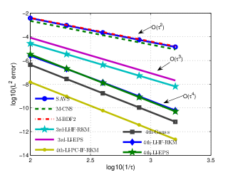
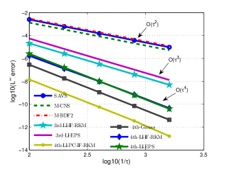
Fig. 1: Time step refinement tests using the different numerical schemes for the 1D Schrödinger equation (1.1).

Then, to demonstrate the advantages of the proposed high-order schemes with the existing schemes, we investigate the global $L^{2}$ errors and $L^{\infty}$ errors of $\phi$ versus the CPU costs using the different schemes at $T=1$ with the Fourier node 2048. The results are summarized in Fig. 2. As it is seen, for a given global error, we can draw the following observations: (i) the high-order schemes spend much less CPU time than all of second-order schemes and the cost of 4th-LI-PC-IF-RKM is cheapest; (ii) the costs of 3rd-LI-IF-RKM and 4th-LI-IF-RKM are much cheaper than 3rd-LI-EPS and 4th-LI-EPS, respectively; (iii) the cost of 4th-LI-IF-RKM is a little expensive over 4th-Gauss. We thank that on the one hand, at the same time steps, the errors provided by 4th-Gauss are much smaller than 4th-LI-IF-RKM (see Figure 1). On the other hand, at every nonlinear iteration step, the constant coefficient matrix of 4th-Gauss is explicitly solved based on the matrix diagonalization method [51] and FFT, thus it is very cheap.

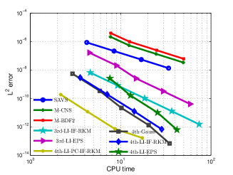
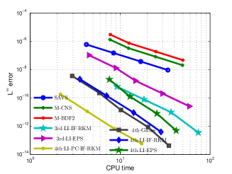
Fig. 2: The numerical errors versus the CPU costs using the different numerical schemes for the 1D Schrödinger equation (1.1).

Subsequently, we investigate the robustness of the proposed schemes in simulating evolution of the soliton as a large time step $\tau=0.1$ is chosen. The results are summarized in Figs. 3-4, where the result provided by 4th-LI-EPS is omitted since the computing result is below-up. It is clear to see that (i) the computational results provided by SAVS, 3rd-LI-IF-RKM and 4th-LI-IF-RKM are wrong; (ii) although M-BDF2, M-CNS and 3rd-LI-EPS can capture the amplitude and waveform, but the small disturbance emergences; (iii) 4th-LI-PC-IF-RKM and 4th-Gauss simulate the soliton well, however, when we set the time step as $\tau=0.2$, the small disturbance emergences for 4th-Gauss (see Fig. 4 (a)), which implies that 4th-LI-PC-IF-RKM is more robust. In addition, based on the results of 3rd-LI-EPS, 4th-LI-EPS, 3rd-LI-IF-RKM and 4th-LI-IF-RKM, we should note that the instability introduced by the extrapolation approximation will be enhanced as the degree of the interpolation polynomial increases, and scuh instability will probably make the proposed scheme invalid as the large time step is chosen. Thus, how to construct an accurate and stable extrapolation approximation need to be further discussed.

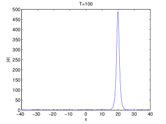
(a) SAVS

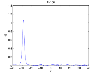
(b) M-BDF2

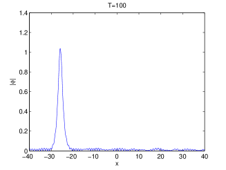
(c) M-CNS

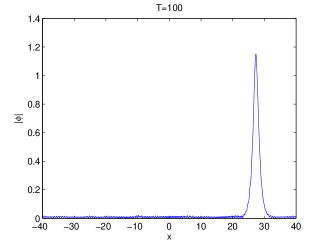
(d) 3rd-LI-EPS

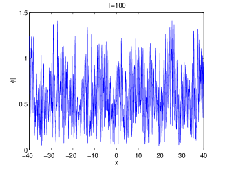
(e) 3rd-LI-IF-RKM

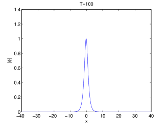
(f) 4th-Gauss

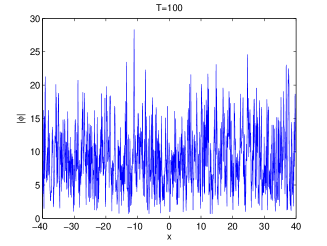
(g) 4th-LI-IF-RKM

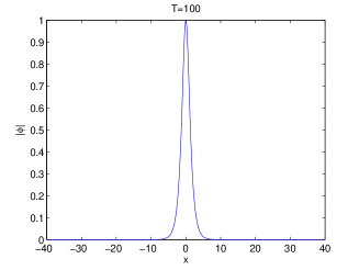
(h) 4th-LI-PC-IF-RKM

Fig. 3: The numerical solution at $T=100$ using the different numerical schemes for the 1D Schrödinger equation (1.1). We take the parameter $\beta=2$, the time step $\tau=0.1$ and Fourier node $N=1024$ and the initial condition is chosen as the exact solution at $t=0$.

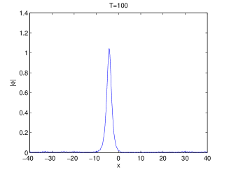
(a) 4th-Gauss

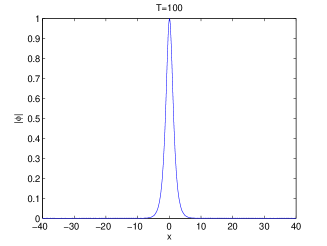
(b) 4th-LI-PC-IF-RKM

Fig. 4: The numerical solution at $T=100$ using the two different numerical schemes for the 1D Schrödinger equation (1.1). We take the parameter $\beta=2$, the time step $\tau=0.2$ and Fourier node $N=1024$ and the initial condition is chosen as the exact solution at $t=0$.

Finally, we visualize the relative residuals on the Hamiltonian energy (3.37), mass (3.38) and quadratic energy (3.10), which are summarized in Fig. 5. We can observe that 3rd-LI-IF-RKM, 4th-LI-IF-RKM and 4th-LI-PC-IF-RKM preserve the quadratic energy exactly and the discrete mass and Hamiltonian energy can be preserved well.

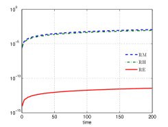
(a) 3rd-LI-IF-RKM

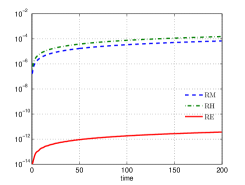
(b) 4th-LI-IF-RKM

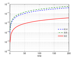
(c) 4th-LI-PC-IF-RKM

Fig. 5: The relative residuals on three discrete conservation laws using the proposed schemes for the 1D Schrödinger equation (1.1). We take the parameter $\beta=2$, time step $\tau=0.01$ and Fourier node 256 and the initial condition is chosen as the exact solution at $t=0$.

4.2 2D nonlinear Schrödinger equation

In this subsection, we employ the proposed schemes to solve the two dimensional (2D) nonlinear Schrödinger equation, which possesses the following analytical solution

$$\phi(x,y,t)=A\exp(\text{i}(k_{1}x+k_{2}y-\omega t)),\ \omega=k_{1}^{2}+k_{2}^{2}-\beta|A|^{2},\ (x,y)\in\Omega.$$

We choose the computational domain $\Omega=[0,2\pi]^{2}$ and take parameters $A=1,\ k_{1}=k_{2}=1$, $\beta=-1$ and $C_{0}=0$. We fix the Fourier node $32\times 32$ so that spatial errors can be neglected here. The $L^{2}$ errors and $L^{\infty}$ errors in numerical solution of $\phi$ at time $T=10$ are calculated by using the three proposed schemes. We take various time steps $\tau=\frac{5\times 10^{-3}}{2^{i}},\ i=0,1,2,3$ for 3rd-LI-IF-RKM and 4th-LI-IF-RKM, and for 4th-LI-PC-IF-RKM, we take various time steps $\tau=\frac{0.2}{2^{i}},\ i=0,1,2,3$. The results are summarized in Fig. 6. It is clear to see that 3rd-LI-IF-RKM is third-order accuracy in time, and 4th-LI-IF-RKM and 4th-LI-PC-IF-RKM have fourth-order accuracy in time, respectively. In Fig. 7, we investigate relative residuals on the mass, Hamiltonian energy and quadratic energy using our schemes, which shows that the proposed schemes can preserve the discrete modified energy (3.10) exactly, and the residuals on the discrete mass and Hamiltonian energy are very small.

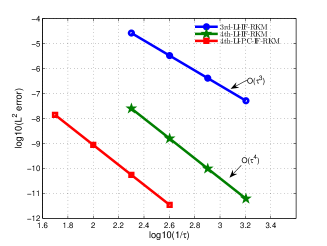
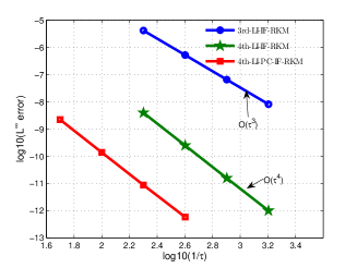
Fig. 6: Time step refinement tests using the three proposed numerical methods for the 2D Schrödinger equation (1.1).

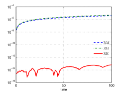
(a) 3rd-LI-IF-RKM

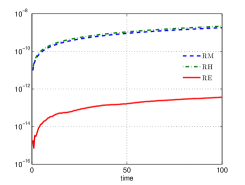
(b) 4th-LI-IF-RKM

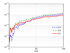
(c) 4th-LI-PC-IF-RKM

Fig. 7: The relative residuals on three discrete conservation laws using the three proposed schemes for the 2D Schrödinger equation (1.1). We take the parameter $\beta=-1$, time step $\tau=0.005$ and Fourier node $32\times 32$, and the initial condition is chosen as the exact solution at $t=0$.

Subsequently, we focus on computing the dynamics of turbulent superfluid governs by the following nonlinear Schrödinger equation

$${\rm i}\partial_{t}\phi({\bf x},t)=-\frac{1}{2}\Delta\phi({\bf x},t)+\beta|\phi({\bf x},t)|^{2}\phi({\bf x},t),\ {\bf x}\in\mathbb{R}^{d},\ d=2,3,\ t>0,$$ (4.2)

with a initial data corresponding to a superfluid with a uniform condensate density and a phase which has a random spatial distribution [4, 38].

Following [4, 38], we choose the computational domain $\Omega=[-10,10]^{2}$ with a periodic boundary condition. By using a similar procedure in [38], the initial data $\phi_{0}$ is chosen as $\phi_{0}(x,y)=e^{{\rm i}\psi(x,y)}$, where $\psi$ is a random gaussian field with a covariance function given by $c(x,y)=e^{-(x^{2}+y^{2})/2}$. The modulus of the solution (i.e., $|\phi|^{2}$) for the dynamics of a turbulent superfluid at different times provided by 3rd-LI-IF-RKM are summarized in Fig. 8. We can clearly see that the phenomenons of wavy tremble are clearly observed at $t=0.3$, and the numerical results are in good agreement with those given in Refs.[4, 38]. Since the modulus of the solution computed by 4th-LI-IF-RKM and 4th-LI-PC-IF-RKM are similar to Fig. 9. For brevity, we omit it here. In Fig. 9 we show the relative residuals on the three conservation laws, which behaves similarly as that given in Fig. 7.

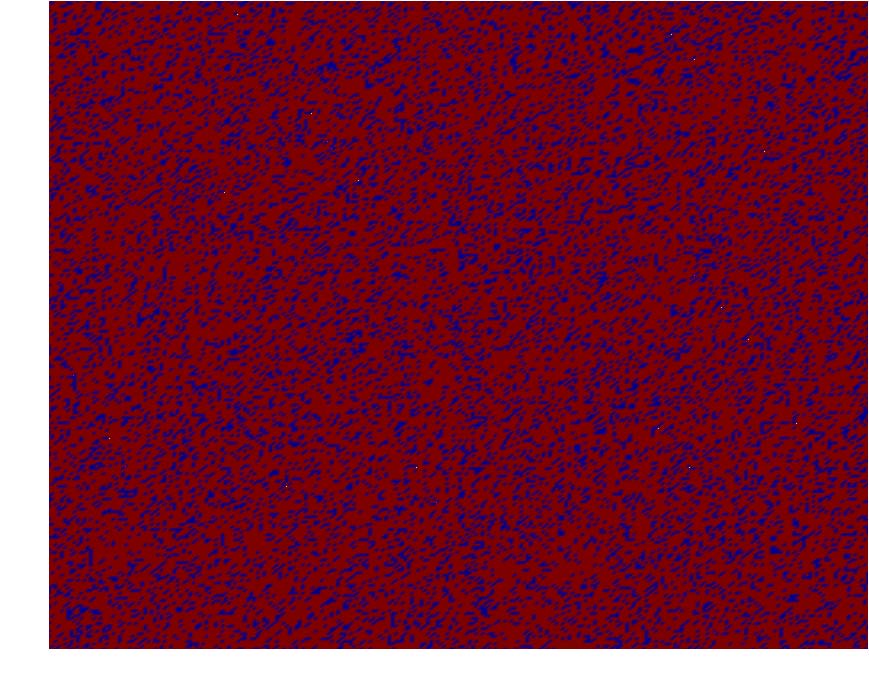
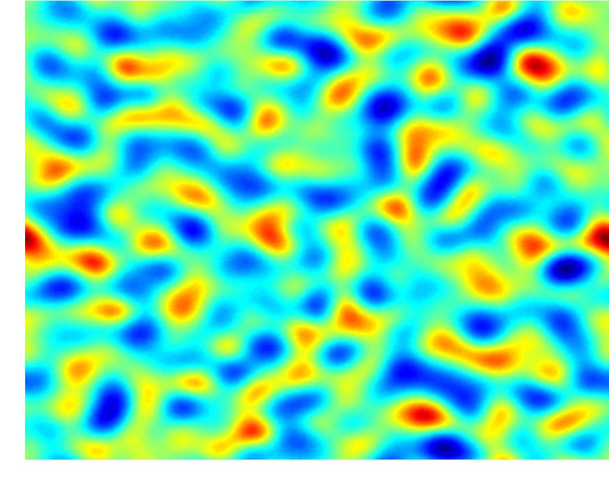
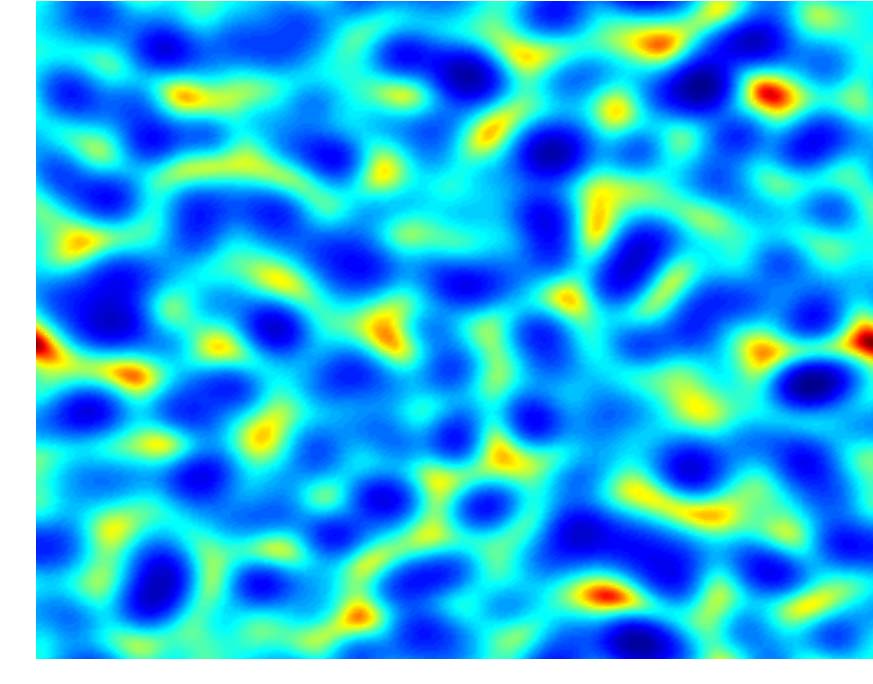
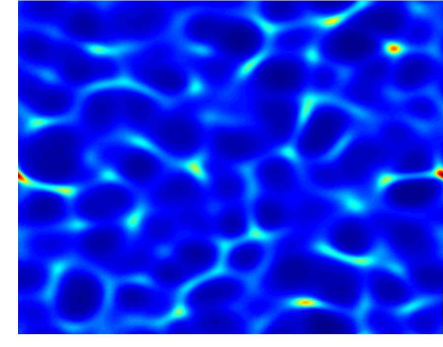
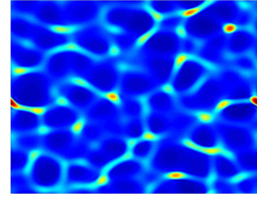
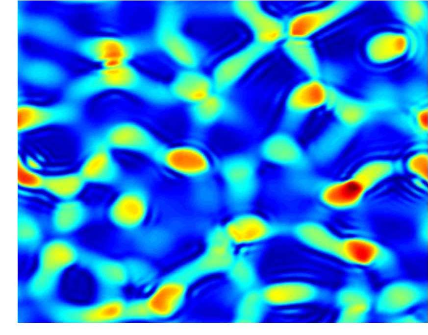
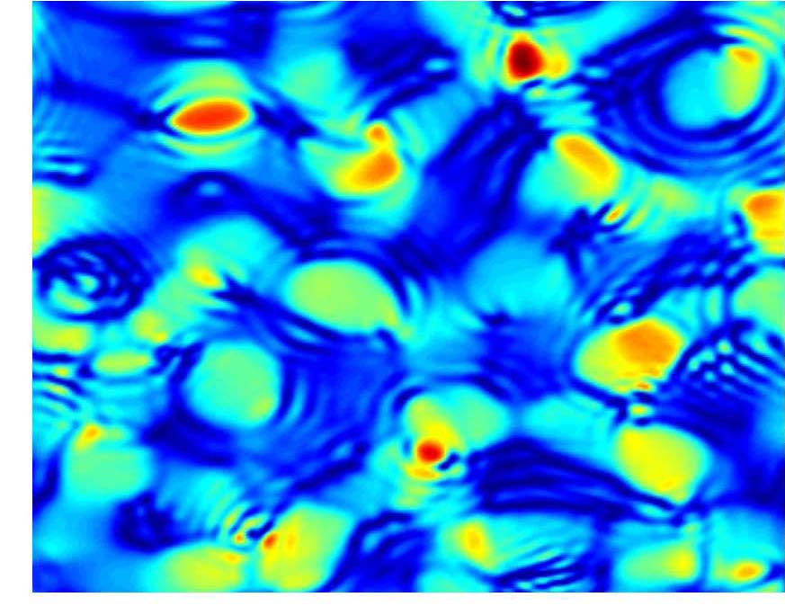
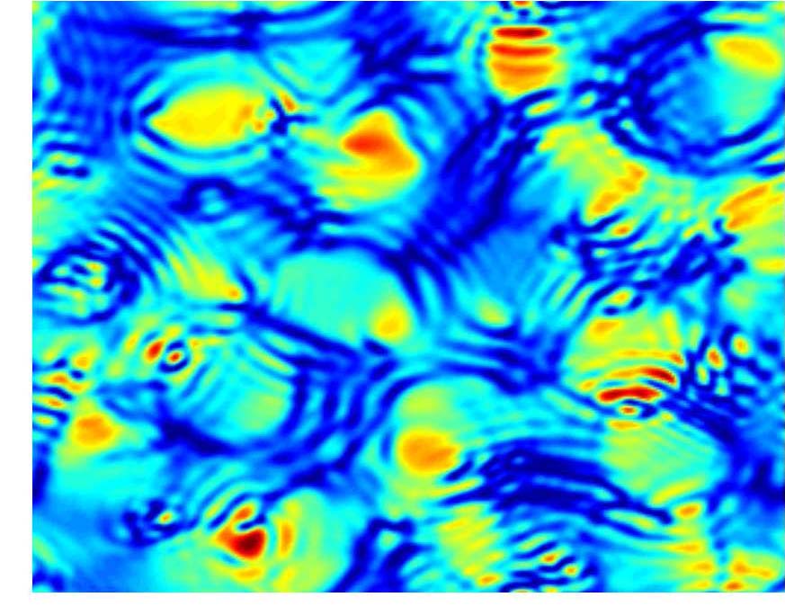
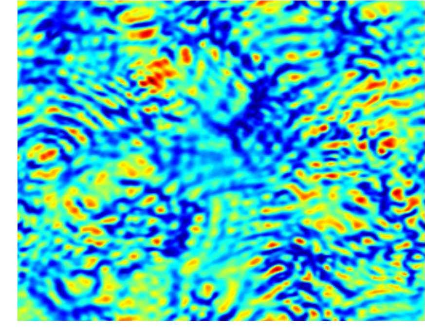
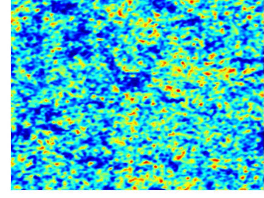
Fig. 8: Modulus of the solution (i.e., $|\phi|^{2}$) for the dynamics of a turbulent superfluid at different times $t=0,0.0005,0.002,0.006,0.01,0.2,0.3,0.4,0.7,5$ (in order from left to right and from top to bottom). We take the parameter $\beta=10$, time step $\tau=0.0001$ and Fourier node $256\times 256$, respectively.

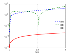
(a) 3rd-LI-IF-RKM

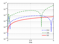
(b) 4th-LI-IF-RKM

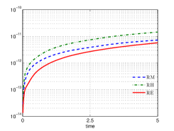
(c) 4th-LI-PC-IF-RKM

Fig. 9: Relative residuals on three discrete conservation laws using the three proposed numerical schemes for the 2D Schrödinger equation (4.2). We take the parameter $\beta=10$, time step $\tau=0.0001$ and Fourier node $256\times 256$, respectively.

4.3 3D nonlinear Schrödinger equation

In this subsection, we use the proposed schemes to solve the three dimensional (3D) nonlinear Schrödinger equation (1.1), which possesses the following analytical solution

$$\phi(x,y,z,t)=\text{exp}({\rm i}(k_{1}x+k_{2}y+k_{3}z-wt)),~{}~{}w=k_{1}^{2}+k_{2}^{2}+k_{3}^{2}-\beta,\ (x,y,z)\in\Omega.$$

We choose the computational domain $\Omega=[0,2\pi]^{3}$ and take parameters $\ k_{1}=k_{2}=k_{3}=1$, $\beta=-1$ and $C_{0}=0$. We fix the Fourier node $16\times 16\times 16$ so that spatial errors can be neglected here. The $L^{2}$ errors and $L^{\infty}$ errors in numerical solution of $\phi$ at time $T=1$ are calculated by using three proposed schemes. We take various time steps $\tau=\frac{5\times 10^{-3}}{2^{i}},\ i=0,1,2,3$ for 3rd-LI-IF-RKM and 4th-LI-IF-RKM, and for 4th-LI-PC-IF-RKM, we take various time steps $\tau=\frac{0.2}{2^{i}},\ i=0,1,2,3$. The results are summarized in Fig. 10. We can observe that 3rd-LI-IF-RKM has third-order accuracy in time, and 4th-LI-IF-RKM and 4th-LI-PC-IF-RKM have fourth-order accuracy in time, respectively. In Fig. 11, we investigate relative residuals on the mass, Hamiltonian energy and quadratic energy by using 3rd-LI-IF-RKM, 4th-LI-IF-RKM and 4th-LI-PC-IF-RKM, respectively, on the time interval $t\in[0,100]$, which behaves similarly as those given in 1D and 2D cases.

Finally, we use our schemes to investigate the dynamics of the 3D nonlinear Schrödinger equation (4.2) (i.e., $d=3$). Inspired by [4, 38], the initial data is chosen to be associated with a superfluid with a uniform density and a random phase, and we take the computational domain $\Omega=[-2,2]^{3}$ with a periodic boundary condition. The modulus of the solution (i.e., $|\phi|^{2}$) for the formation of a 3D turbulent phenomenon at the different times provided by 4th-LI-IF-RKM are summarized in Fig. 12. It can be observed that the vortices filamentation forms gradually during the time evolution. In particular, at time $t=0.8$, the massive vortices filamentation filled to the whole spatial domain, which is consistent with the numerical results presented in [4]. Here, we omit the numerical results computed by 3rd-LI-IF-RKM and 4th-LI-PC-IF-RKM, since they are similar to Fig. 12. The relative residuals on the three conservation laws provided by the proposed numerical schemes are displayed in Fig. 13. As is illustrated in the figure, the proposed schemes can preserve the modified energy exactly and conserve the discrete mass and Hamiltonian energy well.

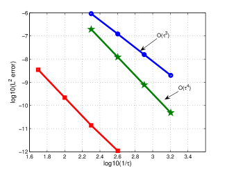
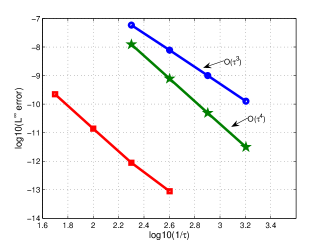
Fig. 10: Time step refinement tests using the three proposed numerical methods for the 3D Schrödinger equation (1.1).

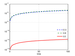
(a) 3rd-LI-IF-RKM

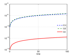
(b) 4th-LI-IF-RKM

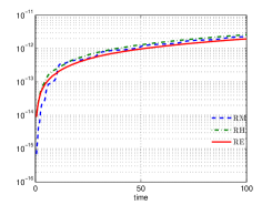
(c) 4th-LI-PC-IF-RKM

Fig. 11: The relative residuals on three discrete conservation laws using the proposed numerical schemes for the 3D Schrödinger equation (1.1). We take the parameter $\beta=-1$, time step $\tau=0.005$ and Fourier node $16\times 16\times 16$, and the initial condition is chosen as the exact solution at $t=0$.

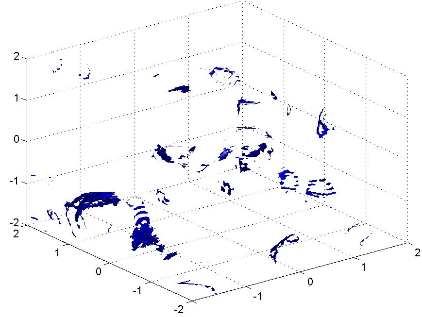
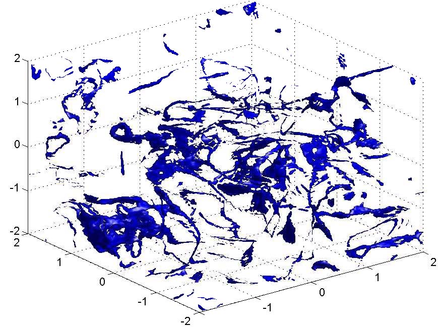
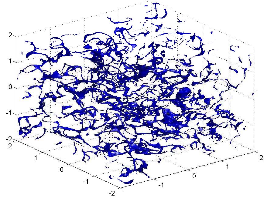
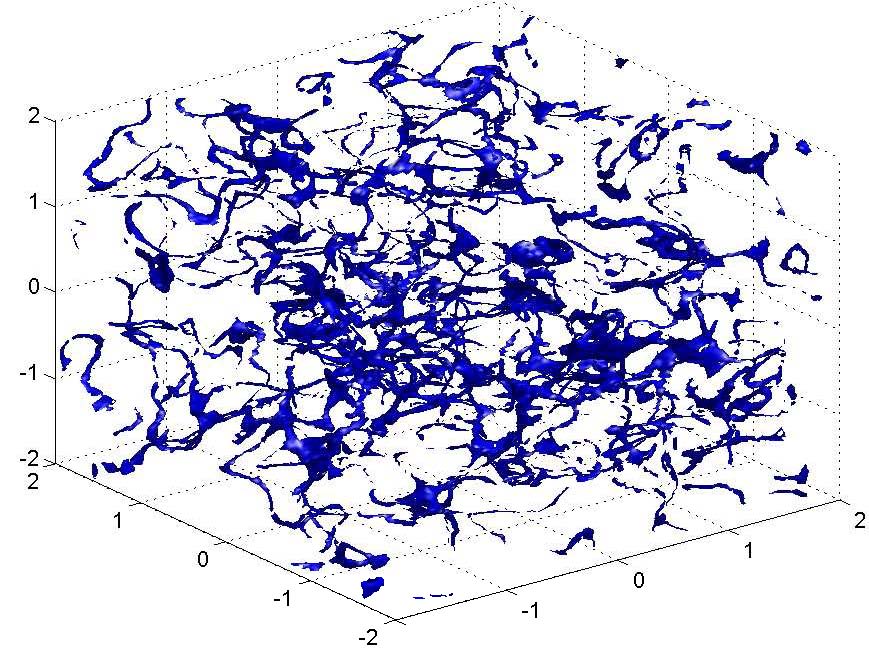
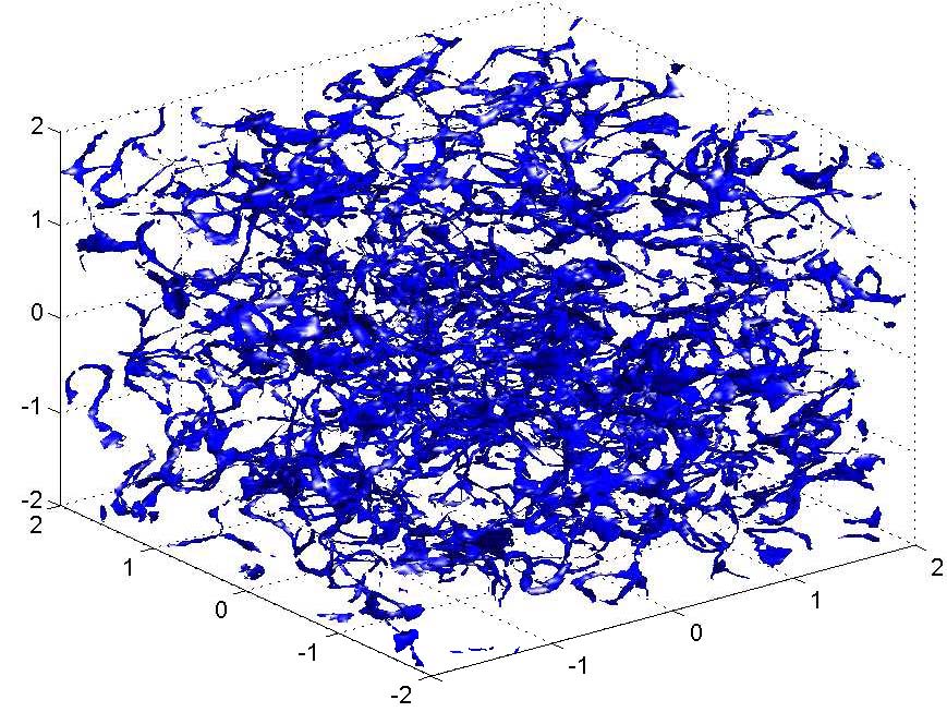
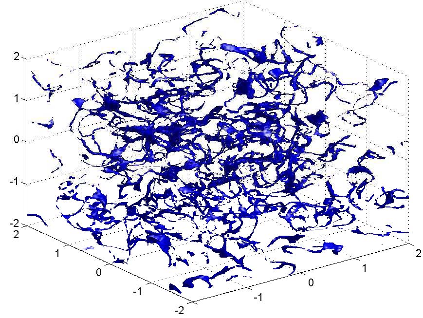
Fig. 12: Turbulence in a superfluid: modulus of the solution (i.e., $|\phi|^{2}$) at different times $t=0.04,0.06,0.5,0.6,0.8,1.0$ (in order from left to right and from top to bottom). We take the parameter $\beta=0.001$, time step $\tau=0.001$ and Fourier node $128\times 128\times 128$, respectively.

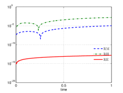
(a) 3rd-LI-IF-RKM

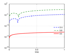
(b) 4th-LI-IF-RKM

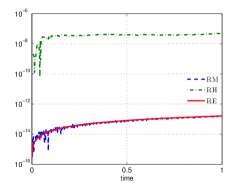
(c) 4th-LI-PC-IF-RKM

Fig. 13: Relative residuals of three discrete conservation laws using the three proposed numerical schemes for the Schrödinger equation (4.2). We take the parameter $\beta=0.001$, time step $\tau=0.001$ and Fourier node $128\times 128\times 128$, respectively.

5 Conclusions

In this paper, based on the Lawson transformation, the Runge-Kutta method and the idea of the SAV approach, we develop a novel class of high-order linearly implicit energy-preserving integrating factor Runge-Kutta methods for the nonlinear Schrödinger equation. The construction of the proposed schemes are two key steps, as follows: (i) We first obtain a linearized system which satisfies a quadratic energy by using the extrapolation technique or prediction-correction strategy to the nonlinear terms of the SAV reformulation; (ii) Then, based on the integrating factor Runge-Kutta method under certain circumstances for the RK coefficients (see (3.9)), a class of linearly implicit energy-preserving schemes are obtained. The proposed scheme can reach high-order accuracy in time and inherit the advantage of the ones provided by the classical SAV approach. Extensive numerical examples are addressed to illustrate the efficiency and accuracy of our new schemes. Compared with some existing structure-preserving schemes, the proposed scheme based on the prediction-correction strategy shows remarkable superiorities. However, we should note that the proposed scheme can only preserve a modified energy and we are sure that the high-order linearly implicit integrating factor Runge-Kutta methods which can preserve original energy will be more advantages than the proposed schemes in the robustness and the long-time accurate computations. Thus, an interesting topic for future studies is whether it is possible to construct high-order linearly implicit schemes which can preserve the original energy.

References

• [1] G. Akrivis, B. Li, and D. Li. Energy-decaying extrapolated RK-SAV methods for the Allen-Cahn and Cahn-Hilliard equations. SIAM J. Sci.Comput., 41:A3703–A3727, 2019.
• [2] G. D. Akrivis, V. A. Dougalis, and O. A. Karakashian. On fully discrete Galerkin methods of second-order temporal accuracy for the nonlinear Schrödinger equation. Numer. Math., 59:31–53, 1991.
• [3] X. Antoine, W. Bao, and C. Besse. Computational methods for the dynamics of the nonlinear Schrödinger/Gross-Pitaevskii equations. Comput. Phys. Commun., 184:2621–2633, 2013.
• [4] X. Antoine and R. Duboscq. Gpelab, a matlab toolbox to solve Gross-Pitaevskii equations II: Dynamics of stochastic simulations. Comput. Phys. Commun., 193:95–117, 2015.
• [5] X. Antoine, J. Shen, and Q. Tang. Scalar Auxiliary Variable/Lagrange multiplier based pseudospectral schemes for the dynamics of nonlinear Schrödinger/Gross-Pitaevskii equations. J. Comput. Phys., 437:110328, 2021.
• [6] W. Bao and Y. Cai. Uniform error estimates of finite difference methods for the nonlinear schrödinger equation with wave operator. SIAM J Numer. Anal., 50:492–521, 2012.
• [7] W. Bao and Y. Cai. Mathematical theory and numerical methods for Bose-Einstein condensation. Kinet. Relat. Mod., 6:1–135, 2013.
• [8] L. Barletti, L. Brugnano, G. F. Caccia, and F. Iavernaro. Energy-conserving methods for the nonlinear Schrödinger equation. Appl. Math. Comput., 318:3–18, 2018.
• [9] C. Besse, S. Descombes, G. Dujardin, and I. Lacroix-Violet. Energy-preserving methods for nonlinear Schrödinger equations. IMA J. Numer. Anal., 41:618–653, 2020.
• [10] Y. Bo, Y. Wang, and W. Cai. Arbitrary high-order linearly implicit energy-preserving algorithms for Hamiltonian PDEs. arXiv, 2011.08375, 2020.
• [11] L. Brugnano and F. Iavernaro. Line Integral Methods for Conservative Problems. Chapman et Hall/CRC: Boca Raton, FL, USA, 2016.
• [12] L. Brugnano, F. Iavernaro, and D. Trigiante. Hamiltonian boundary value methods (energy preserving discrete line integral methods). J. Numer. Anal. Ind. Appl. Math., 5:17–37, 2010.
• [13] M. Calvo, D. Hernández-Abreu, J. I. Montijano, and L. Rández. On the preservation of invariants by explicit Runge-Kutta methods. SIAM J. Sci. Comput., 28:868–885, 2006.
• [14] M. Calvo, A. Iserles, and A. Zanna. Numerical solution of isospectral flows. Math. Comp., 66:1461–1486, 1997.
• [15] E. Celledoni, D. Cohen, and B. Owren. Symmetric exponential integrators with an application to the cubic Schrödinger equation. Found. Comput. Math., 8:303–317, 2008.
• [16] E. Celledoni, V. Grimm, R. I. McLachlan, D. I. McLaren, D. O’Neale, B. Owren, and G. R. W. Quispel. Preserving energy resp. dissipation in numerical PDEs using the “Average Vector Field” method. J. Comput. Phys., 231:6770–6789, 2012.
• [17] Q. Chang, E. Jia, and W. Sun. Difference schemes for solving the generalized nonlinear Schrödinger equation. J. Comput. Phys., 148:397–415, 1999.
• [18] J. Chen and M. Qin. Multi-symplectic Fourier pseudospectral method for the nonlinear Schrödinger equation. Electr. Trans. Numer. Anal., 12:193–204, 2001.
• [19] D. Cohen and E. Hairer. Linear energy-preserving integrators for Poisson systems. BIT, 51:91–101, 2011.
• [20] J. Cui, Z. Xu, Y. Wang, and C. Jiang. Mass- and energy-preserving exponential Runge-Kutta methods for the nonlinear Schrödinger equation. Appl. Math. Lett., 112:106770, 2021.
• [21] M. Dahlby and B. Owren. A general framework for deriving integral preserving numerical methods for PDEs. SIAM J. Sci. Comput., 33:2318–2340, 2011.
• [22] M. Delfour, M. Fortin, and G. Payre. Finite differencee solution of a nonlinear Schrödinger equation. J. Comput. Phys., 44:277–288, 1981.
• [23] X. Feng, B. Li, and S. Ma. High-order mass- and energy-conserving SAV-Gauss collocation finite element methods for the nonlinear Schrödinger equation. SIAM J. Numer. Anal., 59:1566–1591, 2021.
• [24] X. Feng, H. Liu, and S. Ma. Mass- and energy-conserved numerical schemes for nonlinear Schrödinger equations. Commun. Comput. Phys., 26:1365–1396, 2019.
• [25] D. Furihata. Finite difference schemes for $\frac{\partial u}{\partial t}=(\frac{\partial}{\partial x})^{\alpha}\frac{\delta{G}}{\delta u}$ that inherit energy conservation or dissipation property. J. Comput. Phys., 156:181–205, 1999.
• [26] Y. Gong, J. Cai, and Y. Wang. Some new structure-preserving algorithms for general multi-symplectic formulations of Hamiltonian PDEs. J. Comput. Phys, 279:80–102, 2014.
• [27] Y. Gong, Q. Wang, Y. Wang, and J. Cai. A conservative Fourier pseudo-spectral method for the nonlinear Schrödinger equation. J. Comput. Phys., 328:354–370, 2017.
• [28] Y. Gong, J. Zhao, and Q. Wang. Arbitrarily high-order linear energy stable schemes for gradient flow models. J. Comput. Phys., 419:109610, 2020.
• [29] E. Hairer. Symmetric projection methods for differential equations on manifolds. BIT, 40:726–734, 2000.
• [30] E. Hairer. Energy-preserving variant of collocation methods. J. Numer. Anal. Ind. Appl. Math., 5:73–84, 2010.
• [31] E. Hairer, C. Lubich, and G. Wanner. Geometric Numerical Integration: Structure-Preserving Algorithms for Ordinary Differential Equations. Springer-Verlag, Berlin, 2nd edition, 2006.
• [32] N. J. Higham. Functions of Matrices: Theory and Computation. SIAM, Philadelphia, 2008.
• [33] M. Hochbruck and A. Ostermann. Exponential integrators. Acta Numer., 19:209–286, 2010.
• [34] C. Jiang, Y. Wang, and W. Cai. A linearly implicit energy-preserving exponential integrator for the nonlinear Klein-Gordon equation. J. Comput. Phys., 419:109690, 2020.
• [35] C. Jiang, Y. Wang, and Y. Gong. Explicit high-order energy-preserving methods for general Hamiltonian partial differential equations. J. Comput. Appl. Math., 38:113298, 2021.
• [36] L. Ju, X. Li, Z. Qiao, and J. Yang. Maximum bound principle preserving integrating factor Runge-Kutta methods for semilinear parabolic equations. arXiv, 2010.12165v1 [math.NA], 2020.
• [37] L. Ju, X. Li, Z. Qiao, and H. Zhang. Energy stability and error estimates of exponential time differencing schemes for the epitaxial growth model without slope selection. Math. Comp., 87:1859–1885, 2018.
• [38] M. Kobayashi and M. Tsubota. Kolmogorov spectrum of superfluid turbulence: Numerical analysis of the Gross-Pitaevskii equation with a small-scale dissipation. Phys. Rev. Lett., 94:065302, 2005.
• [39] L. Kong, P. Wei, Y. Huang, P. Zhang, and P. Wang. Efficient energy-preserving scheme of the three-coupled nonlinear Schrödinger equation. Math. Meth. Appl. Sci., 42:3222–3235, 2019.
• [40] J. D. Lawson. Generalized Runge-Kutta processes for stable systems with large Lipschitz constants. SIAM J. Numer. Anal., 4:372–380, 1967.
• [41] D. Li and W. Sun. Linearly implicit and high-order energy-conserving schemes for nonlinear wave equations. J. Sci. Comput., 83:A3703–A3727, 2020.
• [42] H. Li, Z. Mu, and Y. Wang. An energy-preserving Crank-Nicolson Galerkin spectral element method for the two dimensional nonlinear Schrödinger equations equation. J. Comput. Appl. Math., 344:245–258, 2018.
• [43] X. Li, Gong Y, and L. Zhang. Two novel classes of linear high-order structure-preserving schemes for the generalized nonlinear Schrödinger equation. Appl. Math. Lett., 104:106273, 2020.
• [44] Y. Li and X. Wu. General local energy-preserving integrators for solving multi-symplectic Hamiltonian PDEs. J. Comput. Phys., 301:141–166, 2015.
• [45] Y. Li and X. Wu. Exponential integrators preserving first integrals or Lyapunov functions for conservative or dissipative systems. SIAM J. Sci. Comput., 38:A1876–A1895, 2016.
• [46] T. Matsuo and D. Furihata. Dissipative or conservative finite-difference schemes for complex-valued nonlinear partial differential equations. J. Comput. Phys., 171:425–447, 2001.
• [47] Y. Miyatake and J. C. Butcher. A characterization of energy-preserving methods and the construction of parallel integrators for Hamiltonian systems. SIAM J. Numer. Anal., 54:1993–2013, 2016.
• [48] G. R. W. Quispel and D. I. McLaren. A new class of energy-preserving numerical integration methods. J. Phys. A: Math. Theor., 41:045206, 2008.
• [49] J. M. Sanz-Serna. Runge-Kutta schemes for Hamiltonian systems. BIT, 28:877–883, 1988.
• [50] J. M. Sanz-Serna and J. G. Verwer. Conservative and nonconservative schemes for the solution of the nonlinear Schrödinger equation. IMA J. Numer. Anal., 6:25–42, 1986.
• [51] J. Shen and T. Tang. Spectral and High-Order Methods with Applications. Science Press, Beijing, 2006.
• [52] J. Shen and J. Xu. Stabilized predictor-corrector schemes for gradient flows with strong anisotropic free energy. Commun. Comput. Phys., 24:635–654, 2018.
• [53] J. Shen, J. Xu, and J. Yang. The scalar auxiliary variable (SAV) approach for gradient. J. Comput. Phys., 353:407–416, 2018.
• [54] J. Shen, J. Xu, and J. Yang. A new class of efficient and robust energy stable schemes for gradient flows. SIAM Rev., 61:474–506, 2019.
• [55] X. Shen and M. Leok. Geometric exponential integrators. J. Comput. Phys., 382:27–42, 2019.
• [56] Z. Sun. Numerical methods for pairtial differential equations. Science Press, Beijing, 2005 (in chinese).
• [57] W. Tang and Y. Sun. Time finite element methods: a unified framework for numerical discretizations of ODEs. Appl. Math. Comput., 219:2158–2179, 2012.
• [58] T. Wang, B. Guo, and Q. Xu. Fourth-order compact and energy conservative difference schemes for the nonlinear Schrödinger equation in two dimensions. J. Comput. Phys., 243:382–399, 2013.
• [59] X. Yang, J. Zhao, and Q. Wang. Numerical approximations for the molecular beam epitaxial growth model based on the invariant energy quadratization method. J. Comput. Phys., 333:104–127, 2017.
• [60] F. Zhang, V. M. Pérez-García, and L. Vázquez. Numerical simulation of nonlinear Schrödinger systems: a new conservative scheme. Appl. Math. Comput., 71:165–177, 1995.
• [61] H. Zhang, X. Qian, J. Yan, and S. Song. Highly efficient invariant-conserving explicit Runge-Kutta schemes for the nonlinear Hamiltonian differential equations. J. Comput. Phys., 418:109598, 2020.