Disentangling Geometric Deformation Spaces in Generative Latent Shape Models

Abstract

A complete representation of 3D objects requires characterizing the space of deformations in an interpretable manner, from articulations of a single instance to changes in shape across categories. In this work, we improve on a prior generative model of geometric disentanglement for 3D shapes, wherein the space of object geometry is factorized into rigid orientation, non-rigid pose, and intrinsic shape. The resulting model can be trained from raw 3D shapes, without correspondences, labels, or even rigid alignment, using a combination of classical spectral geometry and probabilistic disentanglement of a structured latent representation space. Our improvements include more sophisticated handling of rotational invariance and the use of a diffeomorphic flow network to bridge latent and spectral space. The geometric structuring of the latent space imparts an interpretable characterization of the deformation space of an object. Furthermore, it enables tasks like pose transfer and pose-aware retrieval without requiring supervision. We evaluate our model on its generative modelling, representation learning, and disentanglement performance, showing improved rotation invariance and intrinsic-extrinsic factorization quality over the prior model.

Figure 1: Depiction of overall framework goal. We factorize the latent deformation space of a given 3D object into rigid pose $z_{R}$, extrinsic non-rigid pose $z_{E}$, and intrinsic shape $z_{I}$, without supervision.

1 Introduction

A major goal of representation learning is to discover and separate the underlying explanatory factors that give rise to some set of data (Bengio et al., 2013). For many objects, such as 3D shapes of biological entities, structuring their representation within a learned model means understanding the different modes of their deformation spaces. For instance, rotating a chair does not affect its category, nor does articulated deformation of a cat alter its identity. In general, different geometric deformations may be semantically distinct, e.g., shape style (Marin et al., 2020), intrinsic versus extrinsic alterations (Corman et al., 2017), or geometric texture details (Berkiten et al., 2017). In other words, for many objects, we can naturally factorize the associated deformation space, based on geometric characteristics.

Such a disentanglement can provide a useful structuring of the 3D shape representation. For example, in a vision context, one could constrain inference of a 3D model from a motion sequence to change in pose, but not intrinsic shape. Or, in the context of graphics, separating shape and pose allows for tasks such as deformation transfer or shape interpolation.

Figure 2: A schematic overview of the combined two-level architecture used as the generative model. A point cloud $P$ is first encoded into $(q,x_{c})$ by a deterministic AE, where $q$ is the quaternion representing the rotation (rigid pose) of the shape, and $x_{c}$ the compressed representation of the input $P$, in its canonical orientation. $(q,x_{c})$ is then further compressed into a latent representation $z=(z_{R},z_{E},z_{I})$ of a VAE. The hierarchical latent variable $z$ has disentangled subgroups in red (representing rotation, extrinsics, and intrinsics, respectively). The intrinsic latent subgroup $z_{I}$ is used to contain the information in the LBO spectrum ${\lambda}$ using an invertible mapping. Both the extrinsic $z_{E}$ and intrinsic $z_{I}$ are utilized to compute the shape $\widehat{x}_{c}$ in the AE’s latent space. The latent rotation $z_{R}$ is used to predict the quaternion $\widehat{q}$. Finally, the decoded representation $(\widehat{q},\widehat{x}_{c})$ is used to reconstruct the original point cloud $\widehat{P}$. The deterministic AE mappings are shown as dashed lines; VAE mappings are represented by solid lines.

In this work, we consider a purely geometric decomposition of object deformations, separating the space into rigid orientation, non-rigid pose, and shape. Our method is based on methods from spectral geometry, utilizing the isometry invariance of the Laplace-Beltrami operator spectrum (LBOS). The LBOS characterizes the intrinsic geometry of the shape; in contrast, we refer to the space of non-rigid isometric deformations of the shape as its extrinsic geometry, in a manner similar to Corman et al. (2017). This decomposition is performed in the latent space of a generative model, using information-theoretic methods for disentangling random variables, resulting in three latent vectors for rigid orientation, pose, and shape. We apply our model to several tasks requiring this factorized structure, including pose-aware retrieval and pose-versus-shape interpolation (for which pose transfer is a special case). See Fig. 2 for an overview of our approach.

We focus on minimizing the supervision required for our model, eschewing requirements for identical meshing, correspondence, or labels. Thus, our method is orthogonal to advances in neural architectures, as it can be applied to any encoder or decoder model. For the same reason, it is also agnostic to the 3D modality (e.g., meshes, voxels, or implicit fields). We include experiments on meshes and point clouds, to showcase the versatility of our method with respect to shape modality, but we choose to focus on the latter, as they are a common data type in computer vision.

Our method builds on a prior model (Aumentado-Armstrong et al., 2019), the geometrically disentangled VAE (GDVAE), with two major algorithmic improvements: (1) we enhance the ability of the network to factorize rotation, and (2) we replace a simple spectrum regressor with a diffeomorphic flow network. For the first point, we investigate two representation learning approaches that allow the model to discern a canonical rigid orientation, with or without assuming aligned training data. The latter change not only guarantees that spectral information is preserved by the mapping (due to the invertibility requirement), but it can be readily applied to generative modelling (due to the tractability of the likelihood calculation) and it permits shape-from-spectrum computations that prevent contaminating learned latent intrinsics with extrinsic information. This allows us to define a better training procedure, in which we use a shape-from-spectrum starting point, instead of the initial input shape, thus ensuring that the latent intrinsics cannot access extrinsics. These two improvements result in superior disentanglement quality, compared to the prior GDVAE model.

2 Background

2.1 Rotation Invariant Shape Representation

Invariance to rotation is generally a desirable property of shape representations, since many tasks (such as categorization or retrieval) tend to consider orientation a nuisance variable. Hence, there is a significant body of work on how to learn such rigid invariance.

Classical research includes many types of geometric features, directly computed from input shapes, that are rotation invariant (e.g., Guo et al. (2014)), such as structural indexing (Stein et al., 1992), signature of histogram orientations (Tombari et al., 2010), spin images (Johnson and Hebert, 1999), and point signatures (Chua and Jarvis, 1997). More recently, SRINet (Sun et al., 2019), ClusterNet (Chen et al., 2019a), and RIConv (Zhang et al., 2019) design rotation invariant hand-crafted features that can be extracted from point clouds (PCs), for use in learning algorithms.

Separately, rotation equivariance has been achieved in voxel shapes using group convolutions (Worrall and Brostow, 2018) and spherical correlations (Cohen et al., 2018), which can be utilized to obtain invariance. PRIN (You et al., 2018) computes rotation invariant features for point clouds, but requires the application of convolutions on spherical voxel grids. SPHNet (Poulenard et al., 2019) attains rotation invariance without voxelization, by extending feature signals defined on a shape into $\mathbb{R}^{3}$, and then using a specific non-linear transform of the signal, convolved with a spherical harmonic kernel. Additional network architectures have been applied to modelling equivariances, including tensor field networks (Thomas et al., 2018; Fuchs et al., 2020), graph-theoretic methods (Kondor et al., 2018) and quaternion-based approaches (Zhao et al., 2020; Zhang et al., 2020). See also Dym and Maron (2020) for additional discussions and theoretical analysis.

Other works focus on changing the input and/or utilizing other representation learning techniques, which are more closely related to our work. The PCA-RI model (Xiao et al., 2020) achieves rotation invariance by transforming each shape into an intrinsic reference frame, defined by its principal components, handling frame ambiguity (due to eigenvector signs) by duplicating the input. Info3D (Sanghi, 2020) uses techniques from unsupervised contrastive learning to encourage rotation invariance in the representation, including the ability to handle unaligned data. Li et al. (2019) attain equivariance by rotating each input point cloud by a discrete rotation group. Similar to this, an approximately rotation invariant encoder can be defined by feeding in randomly rotated copies of the input (Sanghi and Danielyan, 2019). We build on this latter approach to define one version of our 3D autoencoder (AE). For our other approach, we utilize Feature Transform Layers (FTLs) (Worrall et al., 2017), which allow us to make latent space rotations equivalent to 3D data space rotations. In both cases, rather than removing rigid transforms from the embedding, we attempt to factorize such transforms out, as part of the deformation space of the object.

More specifically, we consider two general approaches to learning rotation invariant representations, building on related work as noted above. Both methods are modality agnostic (e.g., not requiring spherical voxelization), architecture independent (e.g., not necessitating particular types of convolution), able to avoid information loss in feature extraction, and do not increase the cost of a forward pass (e.g., no duplication of inputs). In this sense, our method is largely orthogonal to architectural improvements for PC processing, as well as the aforementioned approaches to rotation invariance. Indeed, they can be readily applied to other 3D shape modalities. This is because our approaches modify only the latent representation and loss calculation procedure, allowing the use of arbitrary features as input, including rotation invariant ones. Nevertheless, we show that, despite obtaining features from a simple PointNet (Qi et al., 2017), we can still approximately attain rotation invariance without architectural alterations. Finally, the utility of much of the related work above for generative modelling and/or autoencoding is unclear; hence, we choose to use simpler architectures already known to work for these purposes (Achlioptas et al., 2017; Aumentado-Armstrong et al., 2019).

2.2 Shape Analysis via Spectral Geometry

Figure 3: Pose versus shape factorization via LBOS. A t-SNE (van der Maaten and Hinton, 2008) plot of LBOSs from the Dyna dataset (Pons-Moll et al., 2015), with illustrative accompanying point cloud representations for several spectra. Different body shapes are mapped close together, regardless of articulated pose.

Figure 4: Visual explanation of the use of spectral geometry in characterizing intrinsic versus extrinsic shape. We display two rows of animals, showing different intrinsics (first row) and extrinsics (second row), across the columns per inset. The plots show the LBOS $\lambda$ across shapes (indices $i$ range from 1 to 50); notice the lack of variability as extrinsics change.

Any 3D surface can be viewed as a 2D Riemannian manifold $(\mathcal{M},g)$, with metric tensor $g$, which allows the application of differential geometry to shape analysis in computer graphics and vision. One major technique in this area is the use of spectral geometry, which is mainly concerned with the Laplace-Beltrami Operator (LBO), $\Delta_{g}$, and its associated spectrum (i.e., the eigenvalues $\lambda$ of $-\Delta_{g}\phi_{i}=\lambda_{i}\phi_{i}$) for shape processing (Patané, 2016). Use of the spectrum generalizes classical Fourier analysis on Euclidean domains to manifolds, transferring concepts from signal processing to transforms of non-Euclidean geometry itself (Taubin, 1995). The LBO spectrum (LBOS) characterizes the intrinsic properties of a manifold (Lévy, 2006; Rustamov, 2007; Vallet and Lévy, 2008), sufficiently matching human intuition on the meaning of “shape”, to the extent it is considered as its “DNA” (Reuter et al., 2006). Mathematically, intrinsic properties of a shape are those that depend only on its metric tensor, independent of its embedding (Corman et al., 2017); this includes, for example, geodesic distances and the LBOS. Among the most useful advantages of intrinsic shape properties is isometry invariance, meaning intrinsics do not change in response to alterations that do not affect the metric. This includes rigid transforms, as well as certain non-rigid deformations, such as biological articulations (approximately). Algorithms relying on shape intrinsics are therefore able to ignore such deformations (e.g., recognize a person regardless of articulated pose). We show some examples of the intrinsic-extrinsic geometric decomposition provided by the LBOS in Figures 3 and 4. We remark that we also refer to extrinsic shape as non-rigid pose, since this is the most intuitive interpretation for the case of approximately isometrically articulating objects, like animals.

Intrinsic spectral geometry processing has thus yielded numerous useful techniques for vision and graphics, often due to its isometry invariance. This includes semi-localized, articulation invariant feature extraction, such as the heat (Sun et al., 2009; Gebal et al., 2009) and wave (Aubry et al., 2011) kernel signatures, later extended to learned generalizations (Boscaini et al., 2015b). Similar techniques can be applied to a variety of downstream tasks for 3D shapes as well, including correspondence (Rodolà et al., 2017; Ovsjanikov et al., 2012), retrieval (Bronstein et al., 2011), segmentation (Reuter, 2010), analogies (Boscaini et al., 2015a), classification (Masoumi and Hamza, 2017), and manipulation (Vallet and Lévy, 2008). Beyond the standard LBOS, more recent research has also explored localized manifold harmonics (Neumann et al., 2014; Melzi et al., 2018), modifications of the LBO (Choukroun et al., 2018; Andreux et al., 2014), and extrinsic spectral geometry (Liu et al., 2017; Ye et al., 2018; Wang et al., 2017).

While the above applications rely on the spectral intrinsics of existing shapes, the inverse problem seeks to reconstruct a shape from an intrinsic operator (or function thereof), such as the LBO (Boscaini et al., 2015a; Chern et al., 2018; Huang et al., 2019). In particular, the shape-from-spectrum (SfS) task seeks to recover a shape from its LBOS, an instance of an “inverse eigenvalue problem” investigated in other fields (e.g., (Chu and Golub, 2005; Panine and Kempf, 2016)). This enables useful spectral-space tasks, such as shape style transfer and correspondence matching (Cosmo et al., 2019; Marin et al., 2021). Fortunately, despite theoretical results suggesting such recovery is not always possible, due to the existence of non-isometric isospectral shapes (i.e., “one cannot hear the shape of a drum”) (Kac, 1966; Gordon et al., 1992), it appears practically possible in many circumstances (Cosmo et al., 2019; Panine and Kempf, 2016). Indeed, Cosmo et al. (2019) show several applications of their approach to SfS recovery, though it is computationally costly and difficult to constrain. More recently, Rampini et al. (2021) utilize spectral perturbations to define universal geometric deformations, while Moschella et al. (2022) apply a learning framework to process unions of partial shapes in the spectral domain. Closest to our work, Marin et al. (2020, 2021) apply a data-driven approach to the SfS problem, among other tasks.

In this work, we focus on utilizing the classical LBOS as a purely intrinsic characterization of the shape. By exploiting the approximate articulation invariance conferred by its isometry invariance, we gain access to a signal that can separate intrinsic shape from articulated pose, without supervision beyond the geometry itself. While the LBO has been used to perform disentangled shape manipulations in the context of computer graphics and vision, such as isometric shape interpolation (Baek et al., 2015), spectral pose transfer (Yin et al., 2015), and shape-from-spectrum recovery (Cosmo et al., 2019), we show how to do such manipulations within a generative model, as a byproduct of the learned representation.

2.3 Learning Shape-Pose Disentanglement

A common task that has been tackled in the context of computer graphics is pose transfer. Utilizing a small set of correspondences, an optimization-based approach can be applied to perform deformation transfer (Sumner and Popović, 2004). Later work utilized the LBO eigenbases to perform pose transfer (Kovnatsky et al., 2013; Yin et al., 2015), via exchanging low-frequency coefficients of the manifold harmonics. In our work, we use the LBOS instead, which avoids issues of basis computation and spectral compatibility (Kovnatsky et al., 2013). Basset et al. (2020) consider transferring shape instead of pose; due to our symmetric formulation, our approach is also capable of this. We refer to Roberts et al. (2020) for a survey of related work.

Recently, several works have attacked pose transfer from a machine learning point of view. Gao et al. (2018) present a method for mesh deformation transfer using a cycle consistent GAN and a visual similarity metric, but require retraining new models for each source and target set. Levinson et al. (2019) utilize a mesh VAE, which relies on data having identical meshing, to separate pose and shape via batching with identical pose and shape labels. LIMP (Cosmo et al., 2020) disentangles intrinsic and extrinsic deformations in a generative model, utilizing a differentiable geodesic distance regularizer; identical meshing or labels are not required, though correspondence is. Zhou et al. (2020) devise a method for separating intrinsics and extrinsics using corresponding meshes known only to have the same shape but different pose, and applying a powerful as-rigid-as-possible geometric prior. Similarly, Fumero et al. (2021) make use of data pairs with shared transforms to obtain a general disentanglement mechanism. Su et al. (2021) also use identity-based semantic supervision, but with an adversarial mechanism on point clouds. Finally, Marin et al. (2020) consider learning a bijective mapping of the LBOS as well, examining its use in the context of neural networks for several tasks, including spectrum estimation from point clouds and shape style transfer; however, they do not focus on deformation space factorization or generative representation learning. Followup work (Marin et al., 2021) investigates shape-from-spectrum tasks, as well as shape-pose disentanglement via optimization.

In our work, we focus on learning a generative representation that factorizes the latent deformation space into intrinsic shape and extrinsic pose, without supervision. We do not require labels (e.g., identity, pose, or shape), identical meshing, correspondence, or even rigid alignment – only the raw geometry, which we use to compute the LBOS. Rather than targeting pose transfer specifically, in our model, the ability to transfer articulation arises naturally from the learned representation. In particular, we build on the GDVAE model (Aumentado-Armstrong et al., 2019), which disentangles shape and pose into two continuous and independent latent factors. Our method, which we refer to as the GDVAE++  model, includes adding a bijective mapping from an LBO spectrum to the space of latent intrinsics, and defining a new training scheme based on this function. We show that the resulting model is significantly improved in terms of disentanglement.

3 Autoencoder Model

Our model consists of two components: an autoencoder (AE) on the 3D shape data and a variational autoencoder (VAE) defined on the latent space of the AE. We show an overview of the complete framework in Fig. 2.

In this work, the AE is used to map a 3D point cloud (PC) to a latent vector, and then decode it back to a reconstruction of the original input. In contrast to the AE used in the prior GDVAE model (Aumentado-Armstrong et al., 2019), we specifically consider the rotational invariance properties of the AE architecture.

Notation.

We assume our input is a PC $P\in\mathbb{R}^{N_{p}\times 3}$, which we want to reconstruct as $\widehat{P}\in\mathbb{R}^{N_{p}\times 3}$. To do so, we encode $P$ into a rigid rotation, represented as a quaternion $q\in\mathbb{R}^{4}$, and canonically oriented non-rigid latent shape, $x_{c}\in\mathbb{R}^{n}$, using learned mappings $E_{r}$ and $E_{x}$. We can also obtain a canonical PC, $P_{c}=D(x_{c})\in\mathbb{R}^{N_{p}\times 3}$, via a decoder $D$. The details for obtaining this rigid versus non-rigid factorization are given below.

3.1 Autoencoder Architecture

We consider two possible AE architectures on PCs. Both models attempt to regress a rotation matrix and a rotation invariant latent shape representation from an input. The first type, which we denote “standard” (STD), uses a straightforward reconstruction loss, but also includes a random rotation before attempting to encode the shape, inspired by prior work (Sanghi and Danielyan, 2019; Li et al., 2019). The second type relies on feature transform layers (FTLs) (Worrall et al., 2017) to learn a latent vector space that transforms covariantly with the 3D data space under rotation, thus allowing the model to learn how to “derotate” to a canonical representation (denoted “FTL-based”).

Implementation-wise, we use PointNet (Qi et al., 2017) to encode an input point cloud, $P$ (which allows us to handle dynamic PC sizes), and fully connected layers (with batch normalization and ReLU) for all other learned mappings, unless otherwise specified. See Appendix §F.1 for details.

3.1.1 Standard Architecture

Figure 5: STD AE architecture. Our standard AE encodes an input PC $P$ into a rigid pose component (quaternion $q$) and canonically oriented shape embedding $x_{c}$. Before passing $P$ to the shape encoder $E_{x}$, a random rotation $\widetilde{R}$ is sampled and applied. The decoder $D$ then generates the canonical PC $P_{c}$, which is rotated by $R(q)$ into the final reconstruction $\widehat{P}$.

Let $P$ be an input PC, that has potentially undergone an arbitrary rotation. We learn two mappings as our encoder, $E_{r}$ and $E_{x}$, which map $P$ to a quaternion $q=E_{r}(P)$ and a latent shape embedding $x_{c}=E_{x}(P)$. Our decoder $D$ generates a canonically oriented PC $P_{c}=D(x_{c})$, which can be rotated to match the input via $\widehat{P}=P_{c}R(q)$, where $R(q)$ is the parameter-less conversion from quaternion to rotation matrix. Inspired by (Sanghi and Danielyan, 2019; Li et al., 2019)), we insert an additional layer before $E_{x}$ that randomly rotates $P$ (i.e., $x_{c}=E_{x}(P\widetilde{R})$, $\widetilde{R}$ being a random sample), to further encourage learning rotation invariant features. We only do this for the standard architecture, shown in Fig. 5.

3.1.2 FTL-based Architecture

We also consider a slightly more complex architecture with a latent space designed for interpretability under rotation transformations, using a Feature Transform Layer (FTL) (Worrall et al., 2017). Several methods have utilized latent-space rigid transforms for mapping 3D data between views (Rhodin et al., 2018, 2019; Chen et al., 2019d, c). Our design is in particular inspired by prior work that extracts canonical representations in the context of 3D human pose using FTLs (Remelli et al., 2020). Nevertheless, the architecture components of the FTL-AE are nearly the same as those of the STD-AE.

Rotational Feature Transform Layers.

The main idea behind FTLs is to view a latent vector $x\in\mathbb{R}^{n}$ as an ordered set of subvectors $U(x)=(u(x)_{1},\ldots,u(x)_{N_{s}})\in\mathbb{R}^{N_{s}\times 3}$, where $N_{s}=n/3$ and $u(x)_{i}\in\mathbb{R}^{3}$, by simply folding it into a matrix. Consider rotating a point cloud $P\in\mathbb{R}^{N_{p}\times 3}$ by a 3D rotation operation $R\in\mathbb{R}^{3\times 3}$, to get a new shape $PR$. By folding, one can analogously perform this rigid transformation on a “latent point cloud”, as $U(x)R$. Ideally, applying $R$ to $P$ or $U(x)$ has the same effect (i.e., rotates the underlying shape in the same way), resulting in an interpretable latent space, with respect to rotation. We define the rotational feature transform layer $F(R,x)=U^{-1}(U(x)R)$ as a latent rotation $R$ of the subvectors of $x$, where the inverse $U^{-1}$ “unfolds” the ordered set of subvectors into a single vector-valued latent variable again (as opposed to the “folding” operator $U$). We will use the FTL mapping $F$ to enforce a rotation equivariant structure onto the latent space, thus allowing us to “derotate” the shape embedding to some canonical rigid pose. We depict the desired duality over rotations in Fig. 6.

Figure 6: Desired commutativity structure of FTL-based architecture. Ideally, latent rotations should have the same effect as in the data space.

Architectural Details.

Figure 7: FTL-based AE architecture. An input PC, $P$, is encoded into a quaternion $q$ and a pose-aware embedding $\widetilde{x}$, representing the rotated (rather than the canonical) shape. The rotational FTL $F$ is then used to de-rotate $\widetilde{x}$ to obtain the canonically oriented shape $x_{c}=E_{x}(P)=F(R(q),\widetilde{x})$. Finally, a reconstruction of the input, $\widehat{P}$, is produced by rotating the decoded canonical PC $P_{c}=D(x_{c})$ using the predicted rigid pose $R(q)$.

Utilizing similar notation to §3.1.1, we first encode $q=E_{r}(P)$, as before, and convert it to a predicted rotation $\widehat{R}=R(q)$. We then compute a non-canonical latent shape $\widetilde{x}=\widetilde{E}_{x}(P)$, which encodes the rotated shape $P$. We then use the FTL to obtain the canonical latent shape via $x_{c}=F(\widehat{R},\widetilde{x})$, which can be decoded via $P_{c}=D(x_{c})$ with shared parameters. As before, we obtain the final reconstruction via $\widehat{P}=P_{c}\widehat{R}$. For notational consistency, we write $E_{x}(P)=x_{c}=F(\widehat{R},\widetilde{E}_{x}(P))$. See Fig. 7 for a visual depiction.

This FTL-based architecture provides greater interpretability in terms of the effect of a rigid transform on the representation; rather than trying to remove the dependence on rotation, we attempt to explicitly characterize it. Rotations in the 3D data space should thus have an identical effect on the resulting latent space representation (and vice versa).

3.2 Autoencoder Loss Objective

The overall loss function for the AE can be written

$$\mathfrak{L}_{\text{AE}}=\mathcal{L}_{c}+\mathcal{L}_{R}+\mathcal{L}_{P}+\mathcal{L}_{x},$$ (1)

where the terms control representational consistency $\mathcal{L}_{c}$, rotation prediction $\mathcal{L}_{R}$, reconstruction $\mathcal{L}_{P}$ and regularization $\mathcal{L}_{x}$. These terms will be different depending on whether one uses the STD-AE (§3.1.1) or FTL-AE (§3.1.2).

3.2.1 Standard Loss Objective

Reconstruction Loss.

The reconstruction loss term for the STD architecture is $\mathcal{L}_{P}=\gamma_{P}D_{P}(P,P_{c})$, where $D_{P}$ includes a Chamfer distance and an approximate Hausdorff loss, similar to prior work (Aumentado-Armstrong et al., 2019; Chen et al., 2019b):

$$D_{P}(P_{1},P_{2})=\alpha_{C}d_{C}(P_{1},P_{2})+\alpha_{H}d_{H}(P_{1},P_{2}),$$ (2)

in which the squared $L_{2}$ distance is used between matched points.

Cross-Rotational Consistency Loss

is a simple loss designed to promote consistency of the latent representation across rotations of the input, i.e., encourage rotation invariance. First, we split each batch into $N_{R}$ copies of the same PCs; we then apply a different random rotation to each copy. Letting $x_{c,i}$ be the embedding of $P$ after having undergone the $i$th rotation, the loss is then

$$\mathcal{L}_{c}=\frac{\gamma_{c}}{M_{c}}\sum_{i=1}^{N_{R}}\sum_{j>i}||x_{c,i}-x_{c,j}||_{2}^{2},$$ (3)

where $M_{c}$ is the number of pairwise distances. Note that, unlike combining features across rotated copies (Xiao et al., 2020; Li et al., 2019), this approach does not increase the computational cost of a forward pass for a single input.

Rotation Loss

depends on whether we assume the data is rigidly aligned or unaligned, i.e., whether we have rotational supervision or not. In the supervised case, where the canonical rigid pose is shared across data examples, we simply predict the real rotation for every example: $\mathcal{L}_{R}=\gamma_{R}d_{R}(R,\widehat{R})$, where

$$d_{R}(R_{k},R_{\ell})=\frac{1}{\pi}\arccos\left(\frac{\text{tr}(R_{k}R_{\ell}^{T})-1}{2}\right)$$ (4)

is the geodesic distance on $SO(3)$ (Huynh, 2009).

In the unsupervised case, we enforce a consistency loss across rotational predictions, which does not rely on a ground truth $P$ being canonical across multiple shapes. Instead, it only asks that the predicted rotations of an object have the same relative difference as the original rotations of the input (which should be true regardless of whether $P$ was originally canonically oriented). Consider rotations of a PC, $P_{i}=P_{0}R_{0}R_{i}$, where our data follows $P=P_{0}R_{0}$, in which $P_{0}$ (the ground truth PC in canonical orientation) and $R_{0}$ (the rotation of the ground truth datum) are both unknown. Our predictions are $\widehat{P}_{i}=P_{c}\widehat{R}_{i}$, so for any two rotations of a single observed PC (e.g., $P_{i}$ and $P_{j}$), we want $\widehat{R}_{i}\approx R_{0}R_{i}$ and $\widehat{R}_{j}\approx R_{0}R_{j}$, meaning we want to predict $R_{k}$ relative to $R_{0}$. Combining these equations means we want $R_{i}^{T}\widehat{R}_{i}\approx R_{j}^{T}\widehat{R}_{j}$ for each such pair. Formally, we write this constraint as

$$\mathcal{L}_{R}=\frac{\gamma_{r}}{M_{c}}\sum_{i=1}^{N_{R}}\sum_{j>i}d_{R}(R_{i}^{T}\widehat{R}_{i},R_{j}^{T}\widehat{R}_{j}),$$ (5)

where $R_{k}$ and $\widehat{R}_{k}$ are the true and predicted rotations for the $k$th copy in the duplicated batch, respectively. As noted above, in the unsupervised case, we do not necessarily wish to regress $R_{i}$ as $\widehat{R}_{i}$, because the initial (derotated) input $P$ is not assumed to be in the canonical orientation of $P_{c}$.

Regularization Loss.

The primary purpose of the AE is to provide a space with reduced complexity and dimensionality, for training the generative VAE model. Following work on learning probabilistic samplers with latent-space generative autoencoders (Ghosh et al., 2019), we apply a small weight decay and latent radius loss: $\mathcal{L}_{x}=\gamma_{w}L_{2}(\Theta)+\gamma_{d}||x_{c}||_{2}^{2}$, where $L_{2}(\Theta)$ is an $L_{2}$ weight decay on the network parameters $\Theta$.

3.2.2 FTL-based Loss Objective

Similar to the network functions, the FTL-AE objective terms, as well as the training regime, are largely reused from the STD-AE. The only major difference is that we compute reconstruction losses for both the instance representation, $\widetilde{x}$, and the canonical representation, $x_{c}$:

$$\mathcal{L}_{P}=\gamma_{\widetilde{P}}D_{P}(P_{r},\widetilde{P})+\gamma_{P}D_{P}(P,P_{c}).$$ (6)

Here, the decoder output $\widetilde{P}=D(\widetilde{x})$ is encouraged to be similar to the rotated input $P_{r}$.

We note that the penalty $\mathcal{L}_{c}$, enforcing consistency of the canonical latent shape vectors $x_{c,j}$ in the FTL architecture, ties the non-canonical embeddings, $\widetilde{x}_{j}$, through an FTL operation (across rotated inputs), as follows:

$$||x_{c,i}-x_{c,j}||_{2}^{2} =||(U(\widetilde{x}_{i})R_{i}-U(\widetilde{x}_{j})R_{j})R_{i}^{T}||_{F}^{2}$$ (7)

$$=||U(\widetilde{x}_{i})-U(\widetilde{x}_{j})R_{j}R_{i}^{T}||_{F}^{2},$$ (8)

where we have used $U(x_{c,k})=U(\widetilde{x}_{k})R_{k}$, and the orthogonality of $R_{k}$ implies $||R_{k}v||_{2}^{2}=||v||_{2}^{2}$ for any $v\in\mathbb{R}^{3}$.

4 Latent Variational Autoencoder Model

4.1 Overview

Our goal is to define a disentangled generative model of 3D shapes, using a VAE. The model should be capable of encoding for representation inference, decoding random noise for novel sample generation, and allowing factorized latent control of intrinsic shape and extrinsic non-rigid pose. The latter decomposition is made possible by use of the LBO spectrum, which allows us to separate non-rigid deformations into intrinsic shape and extrinsic (articulated or non-rigid) pose (see §2.2).

Following Ghosh et al. (2019) and Achlioptas et al. (2017), we use the AE latent space to define our generative model and disentangled representation learning. This allows us to train with much larger batch sizes (useful for information-theoretic objectives based on estimating marginal distribution properties from samples), and generally obtain better computational efficiency. See Fig. 2 for a pictographic overview.

Compared to our prior GDVAE model (Aumentado-Armstrong et al., 2019), we replace a simple predictor of the LBOS from the latent intrinsic shape with a diffeomorphic mapping between the two quantities. This allows us to use the spectrum directly in training (see §4.4) and increase the dimensionality of the latent intrinsics, improving representation performance.

4.2 Model Architecture

4.2.1 Hierarchically factorized VAE

The core of our VAE model is the Hierarchically factorized VAE (HFVAE) model (Esmaeili et al., 2018), which permits penalization of mutual information between sets of vector-valued random variables. This allows us to enforce the latent intrinsics to be separate from the latent extrinsics, specifically.

Let $(q,x_{c})$ be an encoded input from the AE. We define $z_{R}\sim\mathcal{N}(\mu_{R}(q),\Sigma_{R}(q))$, $z_{E}\sim\mathcal{N}(\mu_{E}(x_{c}),\Sigma_{E}(x_{c}))$, and $z_{I}\sim\mathcal{N}(\mu_{I}(x_{c}),\Sigma_{I}(x_{c}))$ to be the latent encodings of the rotation, extrinsic shape, and intrinsic shape, respectively, sampled from their variational latent posteriors. Our decoder is deterministic: $\widehat{q}=D_{q}(z_{R})$ and $\widehat{x}_{c}=D_{x}(z_{E},z_{I})$. All three variables use isotropic Gaussians as latent priors. See Appendix §F.2 for further details.

4.2.2 Normalizing Flow for Spectrum Encoding

In order to encourage $z_{I}$ to hold only shape intrinsics, we utilize the LBOS. In particular, we define an invertible mapping between $\lambda$ and $\mu_{I}$. Let $\widetilde{\mu}_{I}=f_{\lambda}(\lambda)$ be the latent encoding of a real spectrum (i.e., computed from a shape), $\lambda$, and $\widehat{\lambda}=g_{\lambda}(\mu_{I})$ be the predicted spectrum, with $g_{\lambda}=f_{\lambda}^{-1}$. We implement $f_{\lambda}$ as a normalizing flow network (Papamakarios et al., 2019; Kobyzev et al., 2020), defining a bijective mapping between $z_{I}$-space and the space of spectra. For VAE calculations, we use $\widetilde{z}_{I}\sim\mathcal{N}(\widetilde{\mu}_{I},\widetilde{\Sigma}_{I}(\lambda))$.

Briefly, flow networks are specialized neural modules with two general properties: (1) being a diffeomorphic mapping, and (2) having a simple analytic Jacobian determinant. These properties allow tractable exact likelihood computations through the network, via the probability chain rule through each layer (Papamakarios et al., 2019). Many architectures have been proposed with these functional properties (e.g., (Kingma et al., 2016; Kingma and Dhariwal, 2018; Dinh et al., 2016, 2014)) and they have been applied to generative modelling tasks in both 2D and 3D (Kingma and Dhariwal, 2018; Yang et al., 2019), as the tractable exact likelihood allows for stable training of the distribution matching loss to the prior, at the cost of requiring the dimensions of the input and output space to match and restricting the class of allowed neural architectures.

Using a flow mapping ensures that $f_{\lambda}(\lambda)$ can hold complete information about $\lambda$, since the learned network is guaranteed to be diffeomorphic (i.e., it is invertible and differentiable in either direction). Unlike Aumentado-Armstrong et al. (2019), this approach also allows various “shape-from-spectrum” applications (Marin et al., 2020), which we explore in §5.4.2. Thus, the flow network confers an additional benefit, which is the presence of a mapping from $\lambda$-space to $z_{I}$-space, which allows us to define a novel training regime that prevents encouraging the network to store extrinsic information in the $z_{I}$-space for reconstruction, by instead using $\widetilde{\mu}_{I}$ for reconstruction and pushing $\mu_{I}$ to match it (see §4.4). Finally, it has the benefit of being specifically designed for likelihood-based generative modelling, hence its training procedure synergizes well with the HFVAE. In particular, since we want the latent intrinsic space $z_{I}$ to conform to a Gaussian prior (which we enforce with the HFVAE prior-matching losses), we also wish to ensure anything mapped from $\lambda$-space to there does as well. Fortunately, the tractable likelihood of flow networks allows us to directly optimize a prior-matching likelihood, which is not an upper-bound (unlike for VAEs). See §4.3.2 for details.

4.3 VAE Loss Function

The VAE model is trained with the following objective:

$$\mathfrak{L}_{\text{VAE}}=\mathcal{L}_{\text{HF}}+\mathcal{L}_{\lambda}+\mathcal{L}_{F}+\mathcal{L}_{D},$$ (9)

where $\mathcal{L}_{\text{HF}}$ is the hierarchically factorized VAE loss (Esmaeili et al., 2018), $\mathcal{L}_{\lambda}$ measures the likelihood defined by the spectral flow network between spectra $\lambda$ and latent intrinsics $z_{I}$, $\mathcal{L}_{F}$ is a consistency loss between the VAE (mapping between $x_{c}$ and $z$ space) and the flow network, and $\mathcal{L}_{D}$ is an additional disentanglement penalty. We next define the component loss functions used in this complete objective in detail. Note that we assemble two versions of this loss, expounded in §4.4.1 and §4.4.2, which differ in whether to use the latent intrinsics derived from $x_{c}$ or $\lambda$.

4.3.1 HFVAE Loss $\mathcal{L}_{\text{HF}}$

Recall that our latent space $z=(z_{R},z_{E},z_{I})$ is structured, in that we can partition it into three sub-vectors. Our goals are to (1) push $z$ to follow an isotropic Gaussian latent prior and (2) force each component group $z_{g}$, with $g\in\{R,E,I\}$, to be independent from the other two groups, in an information-theoretic sense. Specifically, we use total correlation (TC), a measure of multivariate mutual information, between latent groups to optimize disentanglement (Watanabe, 1960).

Prior work on structured disentanglement (Esmaeili et al., 2018) has shown that the VAE objective can be decomposed in a hierarchical fashion via

$$\mathcal{L}_{\text{HF}}[z]=\; \omega_{R}L_{R}+\beta_{1}\sum_{g}\mathcal{I}_{\text{TC}}[z_{g}]\;+$$

$$\beta_{2}\sum_{d,g}\mathcal{D}_{\text{KL}}[q_{\phi}(z_{g,d})\mid\mid P(z_{g,d})]\;+$$

$$\beta_{3}\mathcal{I}[x_{c},z]+\beta_{4}\mathcal{I}_{\text{TC}}[z]$$ (10)

where $L_{R}$ denotes the reconstruction loss, the $\beta_{1}$ term controls the intra-group total correlation, the $\beta_{2}$ term penalizes the dimension-wise KL-divergence from the latent prior, the $\beta_{3}$ term controls the mutual information between $x_{c}$ and $z$, and the $\beta_{4}$ term controls the inter-group total correlation. The latter term, $\mathcal{I}_{\text{TC}}(z)$, is the most important for our application, as it encourages statistical independence between latent intrinsics and extrinsics – this is our disentanglement objective.

Recall that the VAE input is a quaternion $q$ and canonical shape vector $x_{c}$, while the output are the regressions $\widehat{q}$ and $\widehat{x}_{c}$. The reconstruction loss, $L_{R}$, is written as follows:

$$L_{R}((q,x_{c}),(\widehat{q},\widehat{x}_{c}))=\frac{||x_{c}-\widehat{x}_{c}||_{2}^{2}}{n\,\mathbb{E}[||x_{c}||_{2}^{2}]}+\omega_{q}d_{q}(q,\widehat{q}),$$ (11)

where $n=\text{dim}(x_{c})$, the expected norm $\mathbb{E}[||x_{c}||_{2}^{2}]$ normalizes for differing AEs (making hyper-parameter setting across models easier), and $d_{q}(q_{1},q_{2})=1-|q_{1}\cdot q_{2}|$ is a distance metric on rotations, through unit quaternions $q_{1},q_{2}$ (Huynh, 2009).

4.3.2 Flow Likelihood Loss $\mathcal{L}_{\lambda}$

Since $f_{\lambda}$ is a normalizing flow network and we want to enforce $\widetilde{z}_{I}$ to follow the Gaussian latent prior, we can simply use the standard likelihood objective (Papamakarios et al., 2019; Kobyzev et al., 2020):

$$P_{\lambda}(\lambda)=P_{z_{I}}(f_{\lambda}(\lambda))\,\left|\det\mathcal{J}[f_{\lambda}](\lambda)\right|,$$ (12)

where $P_{z_{I}}$ represents the density of an isotropic Gaussian (latent prior of $z_{I}$) and $\mathcal{J}[f]$ is the Jacobian of $f$. We use a weighted log-likelihood as the final loss: $\mathcal{L}_{\lambda}=-\omega_{p}\log P_{\lambda}(\lambda)$. This loss enforces $\widetilde{z}_{I}$ to follow the latent prior, as in most flow-based generative models. While it is similar to the HFVAE loss on $z_{I}$, it is an exact likelihood (Papamakarios et al., 2019; Kobyzev et al., 2020), rather than a lower bound. As discussed in §4.2.2, this is intuitively possible due to the use of a diffeomorphic transform, constrained to have an computationally tractable Jacobian determinant.

4.3.3 Spectral Intrinsics Consistency Loss $\mathcal{L}_{F}$

We also want the VAE encoder to be consistent with the spectral flow network, so we apply a loss between the spectral and latent intrinsic space outputs:

$$\mathcal{L}_{F}=\omega_{I}||\mu_{I}-\widetilde{\mu}_{I}||_{2}^{2}+\omega_{\lambda}d_{\lambda}(\lambda,\widehat{\lambda}).$$ (13)

$\widetilde{\mu}_{I}=f_{\lambda}(\lambda)$, $\widehat{\lambda}=g_{\lambda}(\mu_{I})$, and $d_{\lambda}$ is a weighted distance between spectra (Aumentado-Armstrong et al., 2019),

$$d_{\lambda}(\lambda,\widehat{\lambda})=\frac{1}{N_{\lambda}}\sum_{n=1}^{N_{\lambda}}\frac{|\lambda_{n}-\widehat{\lambda}_{n}|}{n},$$ (14)

where $N_{\lambda}$ is the number of elements used in the spectrum. This formulation is inspired by Weyl’s estimate (Weyl, 1911; Reuter et al., 2006), which posits approximately linear eigenvalue growth asymptotically. The motivation is to avoid overweighting the higher elements of the spectrum (corresponding to higher geometric frequencies and thus noisier, small-scale shape details). See also Cosmo et al. (2019). Note that this does not assume a particular structure for the LBO, nor for the growth of its eigenvalues; rather, it is a heuristic for reducing the effect of the monotonic growth of $\lambda$ (i.e., non-linear growth will simply change the relative importance of the frequencies in the loss).

4.3.4 Additional Disentanglement Losses $\mathcal{L}_{D}$

Following Aumentado-Armstrong et al. (2019), we utilize two additional losses to promote disentanglement. The first is motivated by Kumar et al. (2017), penalizing the covariance between latent groups:

$$\mathcal{L}_{\Sigma}=\sum_{g\neq\widetilde{g}}\sum_{i,j}\left|\widehat{\Sigma}[\mu_{g},\mu_{\widetilde{g}}]_{i,j}\right|,$$ (15)

where $\widehat{\Sigma}$ is the empirical covariance matrix between latent vectors, computed per batch, and $g,\widetilde{g}\in\{R,E,I\}$. The second takes advantage of the differentiable nature of the networks involved, directly penalizing the rate of change in the intrinsics as the extrinsics are varied (and vice versa). This is implemented as a penalty on the Jacobian between latent groups

$$\mathcal{L}_{\mathcal{J}}=\left|\left|\frac{\partial\widehat{\mu}_{E}}{\partial\mu_{I}}\right|\right|_{F}^{2}+\left|\left|\frac{\partial\widehat{\mu}_{I}}{\partial\mu_{E}}\right|\right|_{F}^{2},$$ (16)

where $\widehat{\mu}_{g}=\mu_{g}(\widehat{x}_{c})$ is the re-encoding of the reconstructed shape from the AE, $\widehat{x}_{c}=D_{x}(z_{E},z_{I})$, such that $\frac{\partial\widehat{\mu}_{g}}{\partial{\mu}_{\widetilde{g}}}=\frac{\partial\widehat{\mu}_{g}}{\partial\widehat{x}_{c}}\frac{\partial\widehat{x}_{c}}{\partial\mu_{\widetilde{g}}}$ for $g\neq\widetilde{g}$ and $\mu_{g}$ is the approximate posterior mean from which $z_{g}$ is sampled. Hence, the final loss term is given by $\mathcal{L}_{D}=\omega_{\Sigma}\mathcal{L}_{\Sigma}+\omega_{\mathcal{J}}\mathcal{L}_{\mathcal{J}}$.

4.4 Training Regimes

We consider two methods of training, which differ in the manner in which the latent variables are obtained at training time. The first is similar to the original Geometrically Disentangled VAE (GDVAE) model, where $z_{I}$ is used for reconstruction and predicting the spectrum. This is the “flow-only” (FO) model. The second takes advantage of the shape-from-spectrum capabilities of the bijective flow mapping, using $\widetilde{\mu}_{I}=f_{\lambda}(\lambda)$ for reconstruction (which does not depend on $x_{c}$), and encouraging $\mu_{I}(x_{c})$ to be close to $\widetilde{\mu}_{I}$. We refer to these models as GDVAE-FO and GDVAE++, respectively. Notice that the latter approach more stringently separates extrinsics and intrinsics, as the decoder has more limited access to extrinsics from $f_{\lambda}(\lambda)$, as opposed to using $x_{c}$. We visualize the two pathways in Fig. 8. Notice that the two training regimes do not differ in their architecture, hyper-parameters, and structure of the forward pass at inference, but only in the structure of the forward pass at training time.

4.4.1 GDVAE-FO Loss

The “flow-only” model is most similar to the prior GDVAE model (Aumentado-Armstrong et al., 2019). We want the encoded intrinsic shape vector $\mu_{I}(x_{c})$ to hold as much information as possible about the spectrum. This is accomplished through the diffeomorphic mapping to $\lambda$ and the spectral losses in $\mathcal{L}_{F}$. In other words, we reconstruct via $\widehat{x}_{c}=D_{x}(z_{E},z_{I})$ and $\widehat{\lambda}=g_{\lambda}(\mu_{I})$. The disentanglement losses $\mathcal{L}_{\text{HF}}$ and $\mathcal{L}_{D}$ are computed with $\mu_{I}$.

Figure 8: Diagram of VAE mappings, depicting the ability to use latent intrinsics derived from $x_{c}$ versus $\lambda$. Black lines indicate mappings always run in training. The blue arrow is used when predicting the latent reconstruction from $x_{c}$ rather than $\lambda$, which is useful at inference time (when $\lambda$ may not be known) and for the GDVAE-FO training scheme (see §4.4). The red arrows depict using latent intrinsics directly procured from the LBOS $\lambda$, as in the GDVAE++ training scheme.

4.4.2 GDVAE ++  Loss

For the GDVAE ++  loss, we use the known spectrum to compute the output latent shape. The idea during training is to enforce the latent intrinsics used for reconstruction (in this case, $\widetilde{z}_{I}$) to only hold intrinsic geometry (using $f_{\lambda}(\lambda)$), and push $z_{I}$ (inferred from $x_{c}$) to be close to it. Thus, $\widehat{x}_{c}=D_{x}(z_{E},\widetilde{z}_{I})$ is used for reconstruction, where $\widetilde{z}_{I}\sim\mathcal{N}(\widetilde{\mu}_{I}=f_{\lambda}(\lambda),\widetilde{\Sigma}_{I}(\lambda))$. In addition, the disentanglement losses $\mathcal{L}_{\text{HF}}$ and $\mathcal{L}_{D}$ are computed with $\widetilde{\mu}_{I}$. Note that this training strategy does not preclude us from processing shapes without spectra at test time, which we do for our evaluations.

5 Experimental Results

5.1 Datasets

Figure 9: Example AE reconstructions and rigid canonicalizations of input point clouds. Per inset, the top row shows input point clouds $P$ under random rotations, while the bottom row displays the resulting canonical decodings $P_{c}$. Colors indicate depth. Architectures used are SMPL-FTL-S, SMAL-FTL-S, and MNIST-FTL-U, respectively (see Table 1). Since MNIST is unsupervised, we rotate the canonical output by a constant rotation for visualization purposes. In particular, notice that the first two MNIST insets (“9” and “6”) are rotated to match (which would be incorrect in the supervised case). We show some failure cases in the last column of each row: for SMPL, the pose (e.g., arms) is incorrectly reconstructed; for SMAL, the hind-legs of the third canonical PC does not match its counterparts, though the overall pose does; for MNIST, the canonical decoding simply fails to match across rotations. Note that we show additional reconstructions (through the VAE) in Fig. 10.

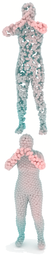
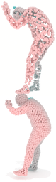
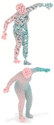
Figure 10: Reconstructions through the VAE. Odd rows are inputs; even rows are reconstructions. Since the model is learned in $x_{c}$-space, reconstruction error manifests as shapes being valid, but slightly off in shape and/or pose (e.g., left-most and right-most insets of top row). All models use the FTL-based AE. See Fig. 9 for qualitative example reconstructions through only the AE. Note that inputs and outputs have the same number of points.

We use the same datasets as in Aumentado-Armstrong et al. (2019). Specifically, we consider MNIST (LeCun et al., 1998), SMAL (Zuffi et al., 2017), and SMPL (Loper et al., 2015). We also assemble a Human-Animal (HA) mixed dataset by combining data from SMAL and SMPL. Note that, in all cases, we perform a scalar rescaling of the dataset such that the largest bounding box length is scaled down to unit length. This scale is the same across PCs (otherwise the change in scale would affect the spectrum for each shape differently). We apply random rotations about the gravity axis (SMAL and SMPL) or the out-of-image axis (MNIST). For rotation supervision, the orientation of the raw data is treated as canonical. We also remark that we use LBOSs derived from the mesh shape, rather than PCs, unless otherwise specified. See Appendix §D for additional dataset details.

Table 1: AE evaluation on held-out test data. Metrics (left to right) refer to the Chamfer distance in reconstructions and the rotational consistency measures (in 3D and $x_{c}$-space, respectively). HA is the humans and animals dataset (SMPL+SMAL). For each model, STD and FTL refer to the type of AE architecture, and U and S denote the use (S) or lack of (U) rotational supervision. For the HA dataset, $a/b$ denote the values on the SMAL and SMPL test sets, respectively. Also, note that, for HA, SMPL shapes are scaled with the SMAL maximum bounding box length; therefore, we scale the Chamfer distances in the evaluations to match the other SMPL models, to make them comparable. $\uparrow(\downarrow)$ means the higher (lower) the better.

Dataset	Model	$d_{C}(P,\widehat{P})\downarrow$	$\mathcal{C}_{\text{3D}}\downarrow$	$\mathcal{C}_{X}\uparrow$
MNIST	STD-U	1.19	1.57	0.92
	FTL-U	0.94	2.73	0.65
SMAL	STD-S	0.35	0.03	0.97
	FTL-S	0.10	0.14	0.93
	STD-U	0.29	0.01	0.97
	FTL-U	0.10	0.21	0.88
SMPL	STD-S	0.34	0.03	0.97
	FTL-S	0.19	0.30	0.71
	STD-U	0.23	0.05	0.97
	FTL-U	0.18	0.45	0.70
HA	STD-S	0.36/0.44	0.03/0.05	0.97/0.97
	FTL-S	0.11/0.19	0.24/0.22	0.66/0.62
	STD-U	0.33/0.34	0.02/0.06	0.97/0.97
	FTL-U	0.11/0.19	0.20/0.20	0.72/0.66

5.2 Autoencoder Results

Our AE is designed to factorize out rigid pose, as well as encode a complete representation of a canonical shape. In Fig. 9, we show example reconstructions, as well as the canonicalization capability of the model. In Fig. 11, we show latent embeddings of the shape representations $x_{c}$ across different rotations of input shapes. The results show that the AE is not only able to accurately reconstruct the inputs, but also correctly derotate the canonical PCs in 3D, and that the encodings are close to being orientation invariant in the latent space.

We consider two AE types, the STD and FTL models with their differing rotation handling techniques. We also examine two ablations: the unsupervised (U) scenario, which removes the assumption of aligned data, and the HA-trained model, which eliminates the use of specialized single models for SMAL and SMPL.

Quantitatively, we evaluate our autoencoders on (1) reconstruction capability and (2) rotation invariance in their representation. Reconstruction quality is computed with the standard Chamfer distance between the output PC and a uniform random sampling from the raw shape mesh. We average over five randomly rotated copies of the test set.

Rotation invariance is assessed with two measures. The first is in 3D space, and checks that canonicalizations of the same PC under different rotations are close (according to the Chamfer distance between PCs):

$$\mathcal{C}_{\text{3D}}=\frac{1}{M_{R}}\sum_{i=1}^{m_{R}}\sum_{j\neq i}d_{C}\left(D(E(P_{i})),P_{j}\right),$$ (17)

where $m_{R}$ is the number of random copies we use for evaluation and $M_{R}$ is the number of pairs tested.

The second measure is in the latent canonical shape space (i.e., $x_{c}$). Since latent distances are less meaningful (e.g., dimensions may have very different scales) and will differ across AEs, we choose to measure performance by clustering quality. Ideally, a representation that canonicalizes an input shape should map rotated copies of a given PC to the same latent encoding – exactly fulfilling this would make it rotation invariant. Hence, we create rotated copies of many input shapes, encode them, and then cluster in the AE embedding space. We expect that rotated copies of the same instance should cluster together; hence, we treat instance identity as a ground truth cluster label and use Adjusted Mutual Information (AMI) to measure quality (Vinh et al., 2010). An AMI of 1 indicates perfect matching of the predicted and real partitions, while an AMI of 0 is the expected value of a random clustering. We average AMIs over clusterings obtained from different random sample sizes (i.e., the number of unique shapes duplicated and clustered). The resulting “area-under-the-curve”-like latent space clustering metric for rotational invariance is denoted $\mathcal{C}_{X}$. See Appendix §C.1 for additional details.

The original GDVAE model (Aumentado-Armstrong et al., 2019) was trained on limited angles of rotation about the canonical one, since otherwise reconstruction quality was degraded but in this work we always consider full rotation about a single axis. Despite the fact that two models use essentially the same architectural components, our AE is better able to obtain canonical orientations, while maintaining reconstruction quality.

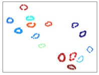
Figure 11: Latent rotational invariance via t-SNE plots of $x_{c}$ vector embeddings. Plots are done with the HA-FTL-U (left) and HA-STD-U (right) models, respectively (see Table 1). Colors denote a single shape; markers with the same color are rotations of that single shape. Marker types are only meant to help tell apart shapes with similar colors. Notice the non-FTL (STD) architecture gives a tighter latent invariance.

The results in Table 1 show a few patterns between the AE types. First, we find the that the FTL-based AE has superior reconstruction quality, while the STD AE has much better rotation invariance. Second, the difference between the unsupervised and supervised scenarios is relatively smaller, with the unsupervised reconstruction quality being slightly better than the supervised, whereas the supervised case has superior rotation invariance. Finally, performance on the HA dataset (which is a union of the SMAL and SMPL data) is only slightly degraded compared to the per-category models (moreso for FTL than STD).

5.2.1 Results Summary

Since the FTL-based AE maintains strong rotation invariance, with superior latent interpretability and reconstruction error, we suggest using it as a starting point. We also find that rotation factorization can be done without aligned data supervision, at little cost to reconstruction or rotational invariance quality.

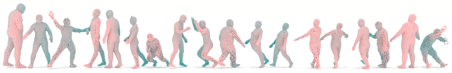
Figure 12: Random sample generations from the VAE. All models use the FTL-based AE. Note that the MNIST model was trained on digits at all orientations and thus should output samples at any orientation (as for SMAL and SMPL). Rows: SMAL, SMPL, MNIST, and HA.

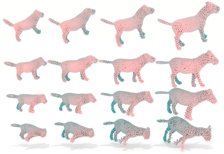
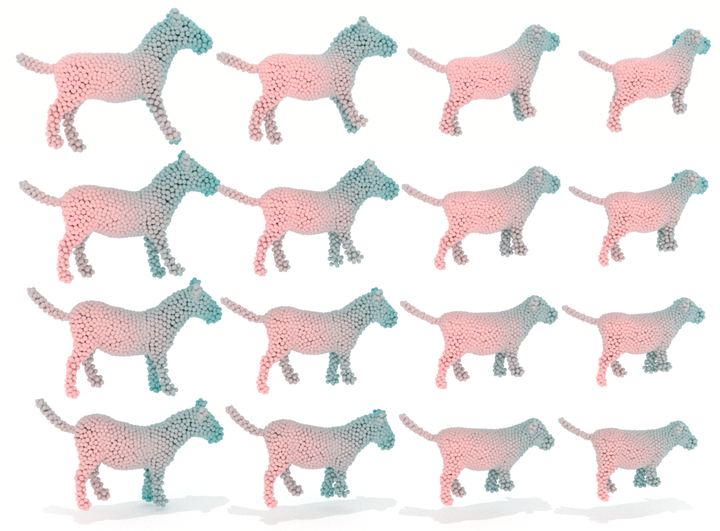
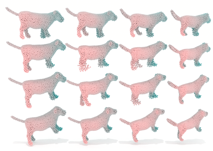
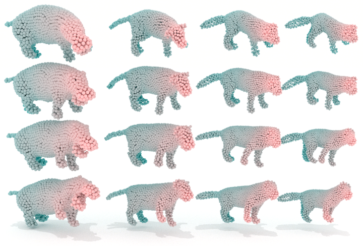
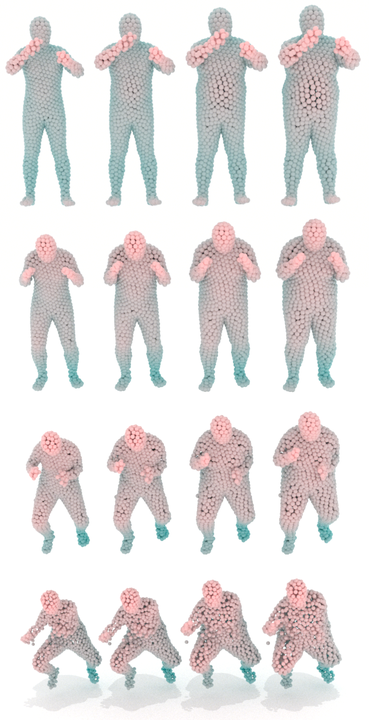
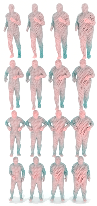
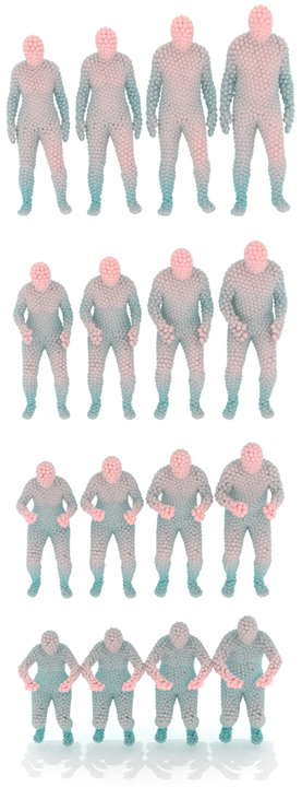
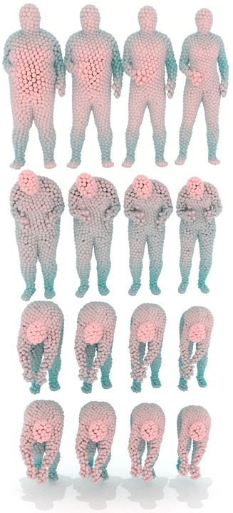
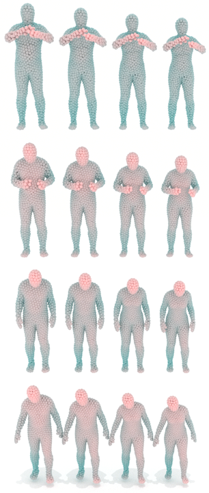
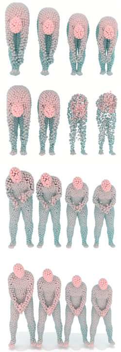
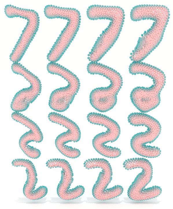
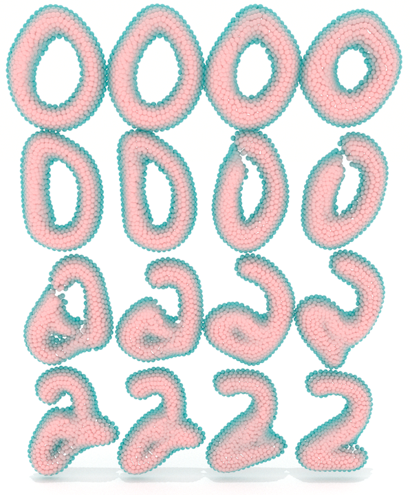
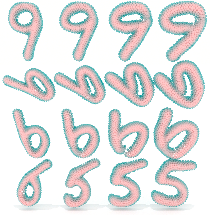
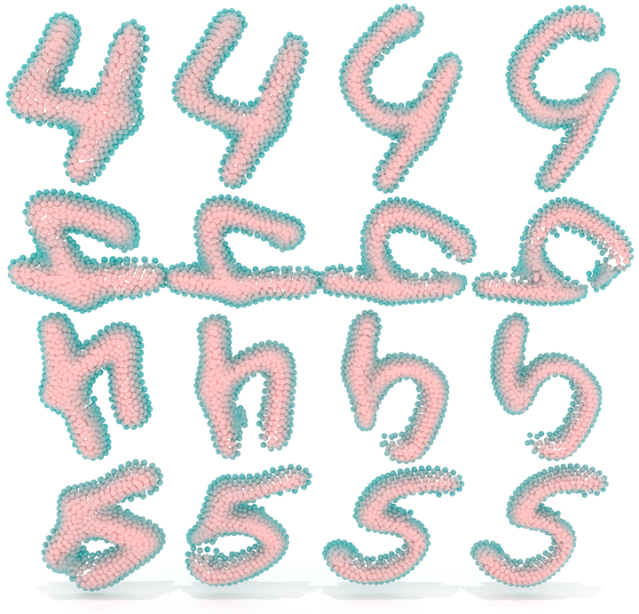
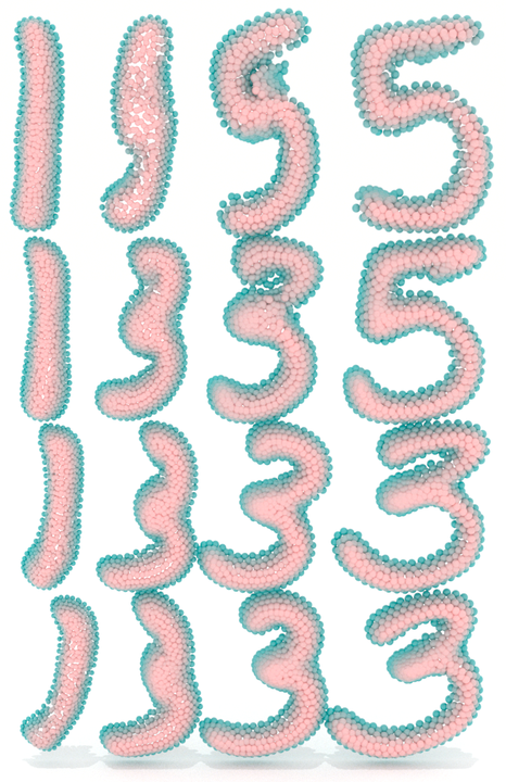
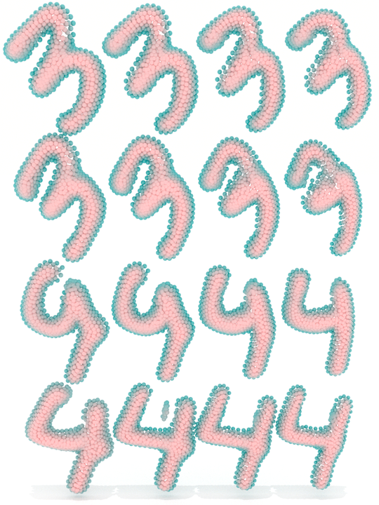
Figure 13: Intrinsic-extrinsic latent space interpolations using the disentangled VAE representation. In each $4\times 4$ panel, top-left and bottom-right shapes are reconstructions of real inputs. Along the horizontal axis, we interpolate along the intrinsics ($z_{I}$), whereas we do so for the extrinsics ($z_{E}$) along the vertical axis. Notice that the bottom-left and top-right shapes are pose transfers, for which one of the latent factors is exchanged, while the other remains unchanged. SMAL and SMPL shapes are shown in the learned canonical orientation (using FTL-S); for MNIST only (using FTL-U), we interpolate the estimated AE rotation encodings $q$ as well, via slerping the quaternions (Shoemake, 1985) between the two inputs along with the extrinsics (i.e., along the vertical axis).

Query	Extrinsic Retrievals (via $z_{E}$)	Intrinsic Retrievals (via $z_{I}$)

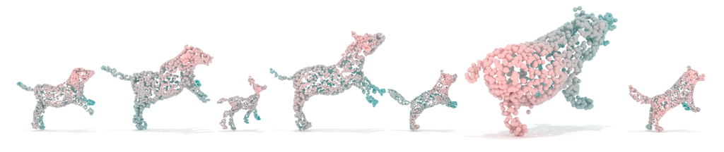
Figure 14: Example retrievals using the disentangled factors of the GDVAE++  latent representation. Shapes are in order of latent similarity from left to right). SMAL, SMPL, and MNIST use FTL-S, FTL-S, and FTL-U AE models, respectively. For SMAL and SMPL, notice that $z_{E}$ retrieves a variety of animals/body types in the same articulated pose, while $z_{I}$ retrieves the same animal/body type in an array of different non-rigid poses. Though MNIST does not have a natural sense of articulation, notice that the extrinsic retrievals tend to have the same digit identity, but vary most noticeably in thickness (which is a non-isometric alteration). In contrast, digits retrieved via $z_{I}$ appear to be bent largely isometrically; that is, “wiggled” around in a way that preserves the metric tensor (and the distribution of geodesic distances among points) – see the “8” digit. For the “6”, notice that it retrieves several “9” digits, showing its blindness to orientation, as well as two “5” shapes that were “thickened” sufficiently in a manner similarly to the query.

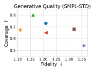
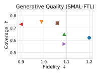
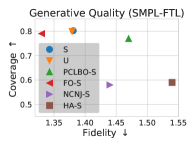
Figure 15: VAE generative modelling evaluation scores on SMAL (left) and SMPL (right) with the FTL AE architecture. Notationally, “S”/“U” refers to the supervised/unsupervised AE settings (see §3.2.1), PCLBO refers to the LBOS being procured from a point cloud (see §5.3.3), NCNJ refers to our disentanglement ablation (see §5.3.4), and HA refers to a model trained on both SMAL and SMPL at the same time (see §5.3). All methods use the GDVAE++ setting (see §4.4), except for the FO case. The upper-left corner of the plots is preferred. See Appendix Table 5 for detailed values. Notice that NCNJ tends to have poor generative quality, while the GDVAE++ (S or U) and GDVAE-FO generally perform well. In most cases, HA underperforms the GDVAE++  (except for the SMAL-FTL case), likely due to the additional complexity of the dataset straining model capacity.

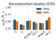
Figure 16: VAE reconstruction quality evaluation, measured in Chamfer distance (lower is better), using the STD (left) and FTL (right) architectures. See Fig. 15 for explanation of model types and Appendix Table 5 for detailed values. We find that the PCLBO and HA models are similar or worse, while NCNJ and FO are similar or slightly better, compared to GDVAE++ (S). Note that NCNJ can take advantage of the weaker disentanglement requirements, while the FO case simply fails to disentangle (see Fig. 17).

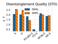
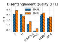
Figure 17: VAE disentanglement quality evaluation (see §5.3.2 and Eq. 18 for discussion of the disentanglement score $\mathcal{S}$). See Fig. 15 for explanation of model types and Appendix Table 5 for detailed values. Compared to the regular GDVAE++, the flow-only (FO) case is severely degraded, whereas PCLBO, HA, and NCNJ experience moderate deterioration (for the latter case, moreso on SMPL than SMAL).

Figure 18: VAE spectral negative log-likelihood (NLL) evaluation, measuring generative quality of the diffeomorphic flow network on the LBOS (see §4.3.2). See Fig. 15 for explanation of model types and Appendix Table 5 for detailed values. In most scenarios, NCNJ experiences some degradation, while NLL in the FO case increases only for the STD case.

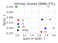
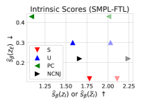
Figure 19: Pose-aware retrieval scores with the FTL AE model. Model notation refers to the GDVAE++ model with (S) or without (U) rotation supervision, use of the PC-derived LBOS (PC; see §5.3.3), and the partial disentanglement loss ablation (NCNJ; see §5.3.4). The lighter (partially transparent) counterparts of each point corresponds to using $\widetilde{z}_{I}=f_{\lambda}(\lambda)$ instead of $z_{I}$ for retrieval. The leftmost two insets show results with SMAL, while the rightmost two do so for SMPL; for each set of two, left and right correspond to scores in intrinsic ($\widehat{s}_{\beta}$) and extrinsic ($\widehat{s}_{\theta}$) retrieval, respectively. Preferred values lie in the bottom-right for intrinsic scores and top-left for extrinsic scores. See Appendix Fig. 22 for plots with the STD AE and Appendix Table 6 for detailed values. We see that (i) using $\lambda$-derived (rather than mesh-derived) latents is consistently better for intrinsic retrieval, but more mixed for extrinsic retrieval (particularly for SMAL); (ii) the PCLBO struggles more on intrinsic than extrinsic retrieval scores (see also §5.3.3); and (iii) removing disentanglement losses (NCNJ) increases the intrinsic score on the extrinsics $\widehat{s}_{\beta}(z_{E})$ (meaning more intrinsic information is erroneously in $z_{E}$), but allows for a modest improvement in extrinsic score $s_{\theta}(z_{E})$, potentially due to the weaker constraints on the latent representation.

5.3 Latent Variational Autoencoder Results

We evaluate our VAE model on three main criteria: (1) representational fidelity, (2) generative modeling, and (3) intrinsic-extrinsic disentanglement. Representational fidelity is captured simply as the reconstruction error, measured via the Chamfer distance between input and output (see Fig. 10 for qualitative examples). To assess generative modeling capability, we utilize the coverage and fidelity metrics (Achlioptas et al., 2017), which examine how well samples from our VAE represent a held-out test set. In addition, utilizing our flow network, we can measure the quality of spectrum generation using the standard log-likelihood. Finally, using the known ground truth intrinsics and extrinsics of our synthetic SMAL and SMPL data, we can measure disentanglement quality via a pose-aware retrieval task. We discuss our results and the details of these metrics in the following sections. Figs. 15, 16, and 17 (as well as Appendix Table 5) show our quantitative results on metrics for all of these criteria.

We explore two variants of our model, using the STD and FTL AEs, as well as several ablations. Two ablations involve the AE: removing rotational supervision (the “S” vs. “U” models) and using only one model for both SMAL and SMPL (via the HA dataset), as opposed to having specialized models for each. Note that the latter scenario not only increases data complexity without altering model capacity, but it also removes some regularities that are present in the independent datasets due to their restricted categories. The remaining ablations affect only the VAE: using a PC-derived LBO (rather than the mesh-derived one we use by default), altering our algorithm to not use the spectrum-derived latent intrinsics in training (GDVAE-FO), and removing the additional disentanglement loss $\mathcal{L}_{D}$ (see §4.3.4).

5.3.1 Generative Modeling

We measure generative modeling quality using the metrics introduced by Achlioptas et al. (2017). Consider two sets of PC shapes: $\varsigma_{G}$, a random set of generated samples, and $\varsigma_{R}$, a set of real PCs. Note that generations are computed via $P=D(D_{x}(z_{E},z_{I}))R(D_{q}(z_{R}))\in\varsigma_{G}$, where $z_{R},z_{E},z_{I}\sim\mathcal{N}(0,I)$ (see §3.1 and 4.2.1). Briefly, we consider two measures: coverage, which checks how well $\varsigma_{G}$ covers the modes of $\varsigma_{R}$ (a proxy for set diversity), and fidelity, which considers how faithful each element in $\varsigma_{G}$ is to its closest counterpart in $\varsigma_{R}$ (a proxy for per-element realism). Coverage is computed by matching each $Q\in\varsigma_{G}$ to its closest PC in $\varsigma_{R}$, and counting the percent of PCs chosen (matched) in $\varsigma_{R}$ (high coverage meaning most of the PCs in $\varsigma_{R}$ are represented in $\varsigma_{G}$). Fidelity (also called minimum matching distance) is computed by matching each $P\in\varsigma_{R}$ to its closest pair in $\varsigma_{G}$, taking the Chamfer distance between them, and averaging these distances over the dataset. Fidelity is needed because coverage does not measure the quality of the matchings (e.g., low quality PCs could be used to cover a given real PC). Matching is always computed as the minimum Chamfer distance. Similar to (Achlioptas et al., 2017), we generate a synthetic set five times larger than the held-out test set, and report the average of running the same evaluation twice. See Fig. 15 for a plot of generative metrics and Appendix Table 5 for quantitative scores. For qualitative visualizations, random sample generations are shown in Fig. 12.

Separately, our flow model $f_{\lambda}$ provides a generative model on LBOSs. Using its bijectivity, we can directly compute the log-likelihood (shown in Fig. 18 and Appendix Table 5). This measures how well our spectral encoder maps real spectra into the Gaussian latent space of the intrinsics.

Looking at Figs. 15 and 18 (as well as Appendix Table 5), we can see that the GDVAE++ and GDVAE-FO score similarly for generative fidelity and coverage, and obtain mixed results on $\log P_{\lambda}(\lambda)$ (the FO method performs better or similar with the FTL AE, but worse with the STD AE), but GDVAE-FO always has better reconstruction results. In terms of AE type, results are mixed, though the FTL approach does tend to have slightly better coverage and worse fidelity. We discuss results related to disentanglement quality in the next subsection.

5.3.2 Shape-Pose Disentanglement

To measure disentanglement quantitatively, we rely on a pose-aware retrieval task in which ground truth continuous values for intrinsics and extrinsics are known.

We start with a set of shapes (SMAL or SMPL) for which parameters for intrinsic shape $\beta$ and extrinsic pose $\theta$ are known. These shapes were not used in training. Let point cloud $P_{i}$ have parameters $(\beta_{i},\theta_{i})$. Using our model, we encode $P_{i}$ into a latent representation $\rho_{i}\in\{x_{c}(P_{i}),z(P_{i}),z_{E}(P_{i}),z_{I}(P_{i})\}$. We then measure distances between representations as $d_{\rho}(P_{i},P_{j})=||\rho_{i}-\rho_{j}||_{2}^{2}$, and rank the retrieved shapes based on $\rho_{i}$. We measure the disentangled retrieval quality for a retrieved PC, $P_{j}$, using query $P_{i}$, by separately checking how well the intrinsic shape and non-rigid pose match. This is done by comparing the query ground truth parameters, $(\beta_{i},\theta_{i})$, to $(\beta_{j},\theta_{j})$, from the retrieved shape.

We compute the distance between these parameters, as the mean squared error between $\beta$ values and the average rotational distance $d_{q}$ across corresponding joint rotations, denoted $E_{\beta}$ and $E_{\theta}$, respectively. Note that we normalize $E_{\beta}$ and $E_{\theta}$ by the mean pairwise error across the dataset for each measure, so that it is relative to the expected error of a uniformly random retrieval algorithm (1 corresponds to random retrieval, while 0 implies obtaining the same parameter set). More specifically, we use the encoding(s) $\rho$ of a PC $P$, to retrieve the three closest shapes (in terms of $d_{\rho}$), and compute the errors $E_{\beta}$ and $E_{\theta}$ averaged over these three retrievals, to obtain two errors per shape. For a fixed encoding type $\rho\in\{x_{c}(P),z(P),z_{E}(P),z_{I}(P)\}$, we get a final error by averaging over an entire held-out test set. Hence, we obtain two scalars $E_{\beta}$ and $E_{\theta}$ for each choice of $\rho$.

We then convert these errors into scores, $s_{\psi}(\rho)=1-E_{\psi}(\rho)$, where $\psi\in\{\theta,\beta\}$. We expect using $z_{E}$ for retrieval (i.e., as $\rho$) to result in a high intrinsic error $E_{\beta}(z_{E})$ (low score $s_{\beta}(z_{E})$), but a low extrinsic error $E_{\theta}(z_{E})$ (high score $s_{\theta}(z_{E})$). Using $z_{I}$ should result in the converse: a high intrinsic score $s_{\beta}(z_{I})$ and a low extrinsic score $s_{\theta}(z_{I})$. We expect retrieval with $x_{c}$ or $z$ to obtain high scores for both parameters.

Lastly, we wish to have a final scalar score that expresses the quality of disentanglement obtained by the model. Notice that $s_{\beta}$ and $s_{\theta}$ are normalized with respect to a random retriever, but are still not comparable (as the errors are originally different units and at different scales). Hence we compute $\widehat{s}_{\psi}(z_{g})={s_{\psi}(z_{g})}/{s_{\psi}(x_{c})}$, with $z_{g}\in\{z,z_{E},z_{I}\}$, normalizing beta and theta retrievals to be in approximately the “same” units (both are errors relative to the AE).

With these normalizations, we make the following interpretations: $\widehat{s}_{\psi}(z_{g})=0$ means that using $z_{g}$ to retrieve shapes is no better (with respect to $\psi$) than random retrieval. In contrast, $\widehat{s}_{\psi}(z_{g})=1$ implies that $z_{g}$ performs just as well as using $x_{c}$; this comparison is relevant, because the AE limits the amount of information available to the VAE. Higher scores (e.g., $\widehat{s}_{\psi}(z_{g})=2$) imply that $z_{g}$ performs $\widehat{s}_{\psi}\times$ better than $x_{c}$ (specifically for retrieving pose alone, when $\psi=\theta$, or intrinsic shape alone, when $\psi=\beta$).

Our normalized retrieval scores $\widehat{s}_{\psi}(z_{g})$ are then used to compute a final disentanglement scalar

$$\mathcal{S}=\widehat{s}_{\beta}(z_{I})+\widehat{s}_{\theta}(z_{E})-\widehat{s}_{\beta}(z_{E})-\widehat{s}_{\theta}(z_{I}).$$ (18)

Higher $\mathcal{S}$ requires accurate extrinsics-based retrieval in terms of pose (high $\widehat{s}_{\theta}(z_{E})$), but poor retrieval (when using $z_{E}$) with respect to intrinsics $\beta$ (low $\widehat{s}_{\beta}(z_{E})$); at the same time, it requires the opposite performance for the latent intrinsics $z_{I}$. Note that random retrieval performance results in all terms being zero (hence $\mathcal{S}=0$); however, one also obtains $\mathcal{S}=0$ if performance for each term is the same as the AE (since all four terms would be one). In other words, good performance retrieving intrinsics (extrinsics) with $z_{I}$ ($z_{E}$) will be cancelled out by good performance retrieving extrinsics (intrinsics) with $z_{I}$ ($z_{E}$). This shows that a high $\mathcal{S}$ requires disentanglement between $z_{E}$ and $z_{I}$.

Disentanglement scores are shown in Fig. 17 (as well as Appendix Table 5). Note that retrieval scores $\mathcal{S}$ are 1.08 and 1.04, for SMAL and SMPL respectively, in the original GDVAE work. As such, the GDVAE++  model obtains significantly superior disentanglement scores across both datasets (including from the HA model) – around double the score of the original model.

From Fig. 19 (as well as Appendix Table 6 and Fig. 22), we also observe the superiority of $\widetilde{z}_{I}=f_{\lambda}(\lambda)$ over $z_{I}$ in retrieving intrinsics, suggesting one should use the spectrum directly when it is available for such a task, though the raw spectrum $\lambda$ cannot be used for other tasks (e.g., smooth interpolation, generation, or same-pose-different-shape retrieval).

Qualitatively, we can assess disentanglement by looking at interpolations within the factorized latent space (shown in Fig. 13). The interpolation plots also show examples of pose transfers (upper-right and lower left corners per inset). For SMAL and SMPL, one can see that the network correctly disentangles articulated pose and shape. For MNIST, where an obvious notion of articulation is not present, moving in $z_{I}$ tends to change digit thickness or allow large-scale shape alterations, while changing $z_{E}$ approximately leaves geodesic distance distributions unchanged (though it can change major factors, like topology).

We can also consider the retrievals qualitatively based on the disentangled latent vectors. Fig. 14 shows what shapes the networks think are most similar to each query, in terms of intrinsics versus extrinsics. We observe that $z_{E}$ is able to retrieve very similar articulations across many animals and/or human body types, while $z_{I}$ correctly retrieves similar shapes without regard for non-rigid pose. For MNIST, retrieval with $z_{E}$ tends to mostly return the same digit with differing thicknesses, while retrieval with $z_{I}$ also largely results in the same digit, but under isometric (non-geodesic-altering) deformations. There are some exceptions to these, such as the nines retrieved by the $z_{I}$ from the six (as the spectrum is unaffected by rotation) or the fives there (potentially due to the closeness of the end of the last stroke in the five to the upper portion of the digit, as well as its thickness, leading to greater intrinsic similarity). The ones retrieved for the eight by $z_{E}$ are less obvious to interpret; they may be due to the low dimensionality of $z_{E}$ or the similarity of ones to thin eights.

We conclude by noting that the GDVAE++ (S or U) generally has the best disentanglement scores (see Fig. 17), while NCNJ has the second-best, but suffers from worse generative quality (Figs. 15 and 18). In comparison, the HA and PCLBO models are generally slightly worse across all metrics (generation, reconstruction, and disentanglement). The FO scenario has by far the worst disentanglement score among all models, underscoring the importance of our altered training regime. While there is some noise (e.g., higher reconstruction error for SMAL-FTL-U in Fig. 16 or superior generative quality for HA on SMAL-FTL in Fig. 15), these trends broadly hold across datasets and AE types (STD and FTL), suggesting our new approach is generally better.

5.3.3 Spectral Robustness

Although we use PCs as our shape representation for these experiments, our spectra are computed on the mesh forms of the shapes, via the cotan weight formulation (Meyer et al., 2003). This provides a useful measure of performance for our model (effectively bounding the performance we can expect with lower quality LBOs), as well as allowing comparison to the original GDVAE model, upon which we are trying to improve. Further, we expect methods for LBOS extraction from PCs to improve over time (e.g., via advances in machine learning (Marin et al., 2021) and geometry processing (Sharp et al., 2021)), making the use of higher quality operators more feasible.

However, for completeness, we also investigated the effect of computing the spectra directly on our subsampled point clouds. This mesh-to-point-cloud conversion process introduces several additional sources of noise: for instance, parts far in geodesic distance may be close in Euclidean space (altering the LBO), and the subsampling of the surface (our PCs being smaller than the number of vertices in SMPL and SMAL) also introduces noise. Hence, we expect results to be degraded, compared to the prior section. For computing the point cloud LBO (PCLBO), we use the robust “tufted” Laplacian operator (Sharp and Crane, 2020).

The scalar disentanglement results are shown in Fig. 17 and Appendix Table 5. While the scores do decrease overall, they are still superior to the scores from the original GDVAE (which used mesh-derived LBOSs to obtain 1.08 and 1.04, for SMAL and SMPL respectively) and the GDVAE-FO models. From Fig. 19 (as well as Appendix Table 6 and Fig. 22), we see that two major terms are negatively affected in the PCLBO case, likely due to noise in the estimated LBOSs: (1) the ability of $z_{I}$ to capture intrinsics degrades, indicated by the decline in $\widehat{s}_{\beta}(z_{I})$, scores; and (2) intrinsic information is not removed as effectively from $z_{E}$, indicated by high values of $\widehat{s}_{\beta}(z_{E})$ (especially for SMPL).

5.3.4 Ablations

Lastly, we consider the effect of ablating two aspects of the model: the additional disentanglement loss $\mathcal{L}_{D}$ and the shape-from-spectrum reconstruction used in the GDVAE++  training.

First, we investigate the utility of the additional disentanglement penalties. By removing these losses, we have no covariance and no Jacobian terms; we denote this scenario NCNJ. For SMAL, the disentanglement scores seem unaffected by this ablation; however, it seems to have introduced a trade-off between reconstruction and generative modelling errors, with $d_{C}$ improving (see Fig. 16), but coverage and $\log P_{\lambda}(\lambda)$ degrading (see Figs. 15 and 18). For SMPL, NCNJ results in degradations in the disentanglement and generative coverage scores (see Figs. 15 and 17). Note that since the VAE prior is Gaussian, it presupposes latent independence (Higgins et al., 2017); hence, disentanglement is likely to affect the prior fitting (and hence generative quality and $\log P_{\lambda}(\lambda)$ as well).

Second, we look at the effectiveness of the “flow-only” training approach, where we do not perform latent shape-from-spectrum during training to perform reconstruction, and instead only use the direct encoding of the AE output. We find that this incurs the most significant degradation in terms of disentanglement score across both datasets (see Fig. 17), showing the importance of using the uncontaminated spectrum for training, rather than relying on the $\mathcal{L}_{F}$ to force $z_{I}$ to carry only intrinsic information. One may notice that, even though GDVAE-FO is similar to the GDVAE model (Aumentado-Armstrong et al., 2019), it has a much lower disentanglement score. This can be partly explained by the increase in dimensionality of the latent intrinsics, as the newer model has a 4-5 times larger $\text{dim}(z_{I})$ than the original GDVAE, making disentanglement more difficult.

5.3.5 Results Summary

The GDVAE++  shows substantial improvements over the original GDVAE model in terms of disentanglement. Using the PCLBO or the combined model (HA dataset) ablations decrease performance, but still maintain this advantage. This improvement also holds regardless of AE type or whether rotational supervision is ablated, showcasing the robustness of our model to AE settings. Much of this gain stems from our shape-from-spectrum training regime: when ablated (the GDVAE-FO model), disentanglement capabilities are crippled.

5.4 Mesh Experiments

The previous results demonstrated the improvements of our approach over the prior GDVAE model. To illustrate applicability to a different 3D shape modality, as well as facilitate comparison to other works, we also tested our method on mesh data.

5.4.1 Human Bodies (AMASS)

Figure 20: Latent interpolations of AMASS validation mesh shapes. As in Fig. 13, per inset, horizontal or vertical movement traverses latent intrinsics $z_{I}$ or extrinsics $z_{E}$, respectively, via linear interpolation. See §5.4.1 for model details. Upper-left and lower-right shapes correspond to real input meshes; upper-right and lower-left shapes therefore correspond to pose transfers.

First, we utilize the AMASS dataset (Mahmood et al., 2019), which combines a number of human motion datasets and provides parametric fitting via SMPL, in order to compare with “Unsupervised Shape and Pose Disentanglement for 3D Meshes” (USPD) (Zhou et al., 2020) on disentangled retrieval and pose transfer tasks.

We alter the AE to (1) process a mesh input, instead of a PC, and (2) output ordered vertex coordinates instead of arbitrary PC sample points. Following other work (Marin et al., 2021; Tan et al., 2018), we use a fully connected encoder. Each output position of the decoder is now semantically associated to a fixed vertex. We alter the loss function to use vertex-to-vertex mean squared error for reconstruction, rather than Eq. 2 (with other terms remaining the same). Notice that we use the vertex correspondence to compute reconstruction loss during the AE training, but this information is not utilized for disentanglement by the VAE, which only has access to latent encodings $x$ in our two-stage training regime. See Appendix §H.1 for details, including hyper-parameter settings.

Table 2: Pose transfer scores (lower is better) on mesh data from AMASS, measured in vertex-to-vertex distance in millimeters (with comparative numbers from Zhou et al. (2020)). Note that the GDVAE model (which outputs a PC) measures error via the more forgiving one-sided Chamfer distance instead (as in Zhou et al. (2020)). See §5.4.1 for additional details. We find that our GDVAE++  outperforms the GDVAE, but underperforms the more strongly supervised USPD, which uses subject labels and mesh correspondence for disentanglement. We mark the GDVAE score with a *, as it is computed with a different (more lenient) metric.

	GDVAE	GDVAE++	USPD
Error $\downarrow$	54.44*	31.54	19.43

Table 3: Pose-aware disentangled retrieval scores on mesh data from AMASS. Note that our latent intrinsics and extrinsics nomenclature refers to the latent “shape” and “pose” (or articulation) vectors in other works. Comparative numbers from Zhou et al. (2020). See §5.4.1 for additional details and Appendix §H.1.3 for empirical standard deviations. We show the difference $\Delta$ between retrieval scores as well ($\widetilde{E}_{\beta}(z_{E})-\widetilde{E}_{\beta}(z_{I})$ and $\widetilde{E}_{\theta}(z_{I})-\widetilde{E}_{\theta}(z_{E})$), such that higher is better. The GDVAE appears to perform well on $\Delta(\widetilde{E}_{\beta})$; however, this is due to the high overall error magnitude in intrinsics retrieval, $\widetilde{E}_{\beta}$. The authors of USPD previously observed a reduction in entanglement when using PCA (measured by $\Delta$); we therefore compare against this dimensionally reduced version as well (using $\dim(z_{I})=5$ and $\dim(z_{E})=15$). We show the best score across categories between the PCA and non-PCA models in bold. In particular, notice that our method underperforms the non-PCA USPD in terms of $\widetilde{E}_{\beta}(z_{I})$ and $\widetilde{E}_{\theta}(z_{E})$, but outperforms it in terms of the $\Delta$ differences; in other words, while USPD retrieves shapes with close intrinsics/extrinsics (when querying with latent intrinsics/extrinsics), those shapes also have similar extrinsics/intrinsics, suggesting a level of shape-pose entanglement remains. In contrast, the PCA-reduced version of USPD has better $\Delta$ values; however, in this case, our PCA-based method has better $\widetilde{E}_{\theta}(z_{E})$, as well as better $\Delta(\widetilde{E}_{\theta})$ overall.

Retrieval with latent:		Intrinsics	Extrinsics	$\Delta$
GDVAE	$\widetilde{E}_{\beta}$	2.80 $\downarrow$	4.71 $\uparrow$	1.91 $\uparrow$
	$\widetilde{E}_{\theta}$	1.47 $\uparrow$	1.44 $\downarrow$	0.03 $\uparrow$
GDVAE++	$\widetilde{E}_{\beta}$	0.41 $\downarrow$	1.36 $\uparrow$	0.94 $\uparrow$
	$\widetilde{E}_{\theta}$	1.15 $\uparrow$	0.80 $\downarrow$	0.35 $\uparrow$
USPD	$\widetilde{E}_{\beta}$	0.14 $\downarrow$	0.92 $\uparrow$	0.78 $\uparrow$
	$\widetilde{E}_{\theta}$	0.94 $\uparrow$	0.76 $\downarrow$	0.18 $\uparrow$
GDVAE++ (PCA)	$\widetilde{E}_{\beta}$	0.50 $\downarrow$	1.49 $\uparrow$	0.98 $\uparrow$
	$\widetilde{E}_{\theta}$	1.21 $\uparrow$	0.82 $\downarrow$	0.40 $\uparrow$
USPD (PCA)	$\widetilde{E}_{\beta}$	0.34 $\downarrow$	2.14 $\uparrow$	1.80 $\uparrow$
	$\widetilde{E}_{\theta}$	1.23 $\uparrow$	0.87 $\downarrow$	0.36 $\uparrow$

We test on two tasks, pose transfer and pose-aware retrieval, on held-out subsets of AMASS. We use the same evaluation methodology and splits as USPD for consistency, which induces minor differences with the evaluations on PCs from previous sections. We first measure pose transfer quality: given two meshes, we can obtain a ground truth transfer by exchanging the SMPL parameters for articulation $\theta$, while fixing those for body shape $\beta$, and obtain our prediction by doing so for $z_{I}$ and $z_{E}$. After decoding, we can measure the average vertex-to-vertex Euclidean distance between the predicted and true transfers. These values are shown in Table 2. While we greatly outperform the original GDVAE, we still underperform USPD for this task. Nevertheless, beyond the additional requirements of USPD (subject labels and vertex correspondence), we note that our VAE is trained to reconstruct AE latent vectors (i.e., it is not trained end-to-end to reduce real-space vertex-to-vertex error), which also potentially contributes to worse performance on this task. In Fig. 20, we show example latent interpolations in the disentangled space, including pose transfers.

We then examine pose-aware retrieval quality. For ease of comparison, we use the error measures on SMPL parameters from USPD: $\widetilde{E}_{\beta}(z_{\psi})=\mathbb{E}_{M_{Q}}||\beta(M_{Q})-\beta(M(z_{\psi}(M_{Q})))||_{2}$ and $\widetilde{E}_{\theta}(z_{\psi})=\mathbb{E}_{M_{Q}}||q(\theta(M_{Q}))-q(\theta(M(z_{\psi}(M_{Q}))))||_{2}$, where $\psi\in\{E,I\}$, $\beta,\theta$ refer to shape and pose SMPL parameters, $M_{Q}$ is a query mesh from a held-out test set, $M(z_{\psi}(M_{Q}))$ is the nearest neighbour mesh to $M_{Q}$ as measured by MSE in $z_{\psi}$ space, and $q$ converts pose angles to unit quaternions. We also examine the differences $\Delta(\widetilde{E}_{\beta})=\widetilde{E}_{\beta}(z_{E})-\widetilde{E}_{\beta}(z_{I})$ and $\Delta(\widetilde{E}_{\theta})=\widetilde{E}_{\theta}(z_{I})-\widetilde{E}_{\theta}(z_{E})$, which should ideally be high. Quantitative results are compiled in Table 3. Compared to USPD, our method has higher $\widetilde{E}_{\beta}(z_{I})$ and $\widetilde{E}_{\theta}(z_{E})$, but outperforms in terms of both differences $\Delta(\widetilde{E}_{\beta})$ and $\Delta(\widetilde{E}_{\theta})$. Intuitively, when querying with latent intrinsics/extrinsics, USPD obtains shapes with very close intrinsics/extrinsics, but those shapes also have similar extrinsics/intrinsics; in other words, some shape-pose entanglement remains. By comparison, the GDVAE++  has less entanglement (higher error when retrieving intrinsics/extrinsics with latent extrinsics/intrinsics), but also higher error in terms of retrieving intrinsics/extrinsics via latent intrinsics/extrinsics.

The authors of USPD also considered a version of their model with reduced dimensionality via PCA, which controlled for the difference in dimensionality between USPD and the GDVAE. They found it had better disentanglement properties, as evidenced by the higher differences $\Delta$, but worse $\widetilde{E}_{\theta}(z_{E})$ and $\widetilde{E}_{\beta}(z_{I})$ values. We observe a similar effect occurs with our model when using PCA to transform $z_{E}$ and $z_{I}$ to that same dimensionality as well (from 9 to 5 for $\dim(z_{I})$ and 18 to 15 for $\dim(z_{E})$). Comparing the PCA-reduced case, USPD has superior retrieval results in terms of intrinsics, but ours has better values in terms of extrinsics ($\widetilde{E}_{\theta}(z_{E})$ and $\Delta(\widetilde{E}_{\theta})$).

We note that these $\Delta$ measures effectively weight the two terms equally, which may not be ideal. However, we find that a uniformly random retrieval algorithm incurs average errors of 6.5 for $\widetilde{E}_{\beta}$ and 1.76 for $\widetilde{E}_{\theta}$ (as well as $\Delta$ values close to zero), suggesting none of these models are actually selecting random intrinsics/extrinsics for given query extrinsics/intrinsics, as one would expect from perfectly disentangled retrieval.

Overall, our model underperforms USPD on pose transfer, but is more competitive on retrieval. However, we remark that USPD relies on known subject identities to obtain sets of people with identical intrinsics, but different extrinsic pose, providing the network with explicit information about the articulated pose space for a given shape. It also utilizes vertex correspondence, which our method does not use for disentanglement. Together, these provide powerful learning signals to the network. This is different than our use of the LBOS, which is specific to a geometric entity, extractable from raw geometry, and not based on semantic knowledge about identity. In other words, USPD performs better for these tasks, but is more specialized, whereas our approach defines a generic structural prior on the deformation space of objects, which happens to disentangle articulation and intrinsic shape as a natural geometric consequence. Other factors, such as our need for low latent dimensionality and inability to do end-to-end training (necessitated by our information-theoretic disentanglement) also contribute to reduced performance.

5.4.2 Human Faces (CoMA)

We also investigated our approach on human face meshes, derived from the CoMA dataset (Ranjan et al., 2018). In particular, we consider the utility of our approach on a shape-from-spectrum task, under identical experimental conditions to recent work by Marin et al. (2021). Given an LBOS $\lambda$, our goal is to reconstruct the original shape $S$. Due to our use of a flow network, we can easily encode $\lambda$, to obtain the latent intrinsics $\widetilde{z}_{I}(\lambda)$. However, we also require latent extrinsics, which we must obtain without access to $S$. Fortunately, our VAE-based formulation permits a straightforward, principled solution: simply use the mode of the Gaussian prior over the latent extrinsics, meaning we set $z_{E}\equiv\vec{0}$. We can then decode $z=(\widetilde{z}_{I}(S),\vec{0})$ to obtain the reconstructed shape $\widehat{S}$ with “mean” extrinsic pose, according to the prior. In practice, if we use more eigenvalues, more of the shape will be represented in $\widetilde{z}_{I}$; for fair comparison, we use the same number as Marin et al. (2021) (i.e., $\dim(\lambda)=30$). Error is simply the vertex-to-vertex Euclidean distance between the meshes $S$ and $\widehat{S}$. Appendix §H.2 contains additional details.

Our results are displayed in Table 4. We consider two nearest neighbour baselines ($\lambda$-NN-$L_{2}$ and $\lambda$-NN-$d_{\lambda}$), which simply retrieve the closest shape in the training set to the given spectrum, using the Euclidean distance or our weighted $d_{\lambda}$ (Eq. 14), respectively. We remark that using $d_{\lambda}$ provides superior retrievals than the $L_{2}$ metric, as it corrects for the growth of the monotonic LBOS, which overweights high frequency geometric details. The method by Marin et al. (2021) outperforms these baselines, but our method (using the mode of the VAE prior for $z_{E}$) performs the best overall. We observe that there is still a performance gap compared to using $z_{E}(x)$ (bottom row of the table); however, this is to be expected, since using the truncated spectrum alone will lose some information.

We also provide example latent interpolations on the CoMA dataset in Fig. 21. Notice that our latent intrinsics capture overall head shape, while the latent extrinsics contain deformations of the mouth and other facial expressions, despite only using raw meshes as input to the algorithm. Compared to Marin et al. (2021), which must perform a regularized optimization to obtain such disentanglement, our method simply linearly interpolates $z_{I}$ and $z_{E}$.

Method	Error $\downarrow$	Spectrum Only
$\lambda$-NN-$L_{2}$	4.47	Yes
$\lambda$-NN-$d_{\lambda}$	2.63	Yes
Marin et al. (2021)	1.61	Yes
$\widetilde{z}_{I}(\lambda)$ & $z_{E}\equiv 0$ (Ours)	1.52	Yes
Full $z$ (Ours)	1.24	No

Table 4: Empirical shape-from-spectrum results on CoMA, following the experimental settings of Marin et al. (2021). Columns: reconstruction methods, test set error (in terms of vertex-to-vertex $L_{2}$ distance), and whether or not some form of information about the shape extrinsics is used. Rows refer to different approaches: $\lambda$-NN-$L_{2}$ simply retrieves the closest shape in the training set, based on the $L_{2}$ distance between LBOSs; $\lambda$-NN-$d_{\lambda}$ is the same nearest neighbour approach, but using our $d_{\lambda}$ metric (Eq. 14) instead (which avoids over-emphasizing high frequency geometric details); “$\widetilde{z}_{I}(\lambda)$ & $z_{E}\equiv 0$” denotes simply setting $z_{E}$ to be zero; and “Full $z$” means $z=(z_{I}(x),z_{E}(x))$ is used, which forms a lower bound on the error we can expect, as it uses both intrinsic and extrinsic information from the full shape $S$. Our approach with $z_{E}\equiv 0$ uses only the spectrum $\lambda$ of the shape (and no other information from $S$ or $x$); it is equivalent to simply choosing $z_{E}$ as the mode of the VAE prior, over the space of latent extrinsics. Overall, our method, which separates latent intrinsics and extrinsics, as well as guarantees invertibility, performs best. For our two VAE-based approaches, we observe a standard error of the mean of 0.02 (using only $\lambda$) and 0.009 (using full $z$). All error values are $\times 10^{-5}$.

Figure 21: Example latent interpolations on the CoMA dataset. Per inset, horizontal movement corresponds to linear changes in $z_{I}$, while vertical movement corresponds to linear changes in $z_{E}$. Upper left and lower right images are starting and ending points; upper right and lower left are thus pose (or intrinsics) transfers. The model is capable of correctly preserving identity when the intrinsics, $z_{I}$, are fixed (i.e., within columns), as well as representing subtle expressions (e.g., the orientation of the mouth in the leftmost inset). We remark that there are a few failure cases (e.g., bottom row of the third inset, top row of the fourth inset) where the non-rigid pose (facial expression) is not exactly preserved as the latent intrinsics change. However note that our formulation demands only that latent shape and extrinsics are disentangled; it does not directly enforce which non-rigid pose should semantically correspond across different intrinsics.

6 Discussion

In this work, we have devised a method for separating the deformation space of an object into rigid orientation, non-rigid extrinsic pose, and intrinsic shape. We require no information other than the geometry of the shapes themselves (i.e., no labels or correspondences). Our method relies on the isometry invariance of the LBOS, which can be estimated from the geometry directly, and uses disentanglement techniques to partition the latent space of a generative model into these independent components.

In particular, we have built upon the GDVAE model (Aumentado-Armstrong et al., 2019) with two primary technical improvements. First, we investigated two approaches to improving rotation factorization: STD, which utilizes randomly rotated inputs to enforce rotation invariance (Li et al., 2019; Sanghi and Danielyan, 2019), and FTL, which provides an interpretable latent space in which 3D rotations in a “folded” latent space mirror the effects of those rotations in real-space (Worrall et al., 2017; Remelli et al., 2020). Compared to the GDVAE, which was only able to maintain robustness to small rotations, both new AEs can handle arbitrary rotations about a single axis; the FTL method has the additional benefit of latent interpretability. Second, we utilized a diffeomorphic normalizing flow network to map between LBOSs and latent intrinsic space. Unlike the GDVAE, which did not have a mapping from LBOS space to latent intrinsic space (and thus could not architecturally stop latent intrinsics $z_{I}$ computed from an encoded shape $x$ from being affecting by extrinsic pose information), utilizing this mapping in our GDVAE++ training procedure (see §4.4) allows us to compute reconstructions through $\widetilde{z}_{I}$ instead, guaranteeing this separation. Further, the bijectivity of the flow ensures that (i) spectral information is not lost and (ii) generative likelihood is tractably computable. Altogether, these changes result in greatly improved unsupervised disentanglement, without sacrificing other representational aspects.

Our results show that we have significantly improved on the GDVAE. Firstly, we are able to handle larger orientation changes with far better robustness in both the 3D data space and latent space (see §5.2), utilizing rotational invariance techniques that do not rely on a specific feature extraction or neural architecture. Secondly, we obtain nearly double the quantitative disentanglement score, for data from both SMAL and SMPL, using our GDVAE++ training scheme (see §5.3.2). We also examined the ability of the model to generate novel shape samples (see Fig. 12), its capacity to smoothly and independently control latent shape and non-rigid pose (see Figs. 13, 20, and 21), and the effect of several ablations and modifications of the model (see §5.3.3 and §5.3.4). Finally, we compare the GDVAE++  to existing techniques for disentanglement and shape-from-spectrum recovery (see §5.4).

For future work, we expect research on localized spectral geometry (Neumann et al., 2014; Melzi et al., 2018), LBO modifications (Choukroun et al., 2018; Andreux et al., 2014), and extrinsic spectral shape (Liu et al., 2017; Ye et al., 2018; Wang et al., 2017) to be potentially useful. Furthermore, our formulation is readily applicable to other 3D shape modalities (e.g., tetrahderal meshes or implicit fields), as the only elements of our architecture that would require alteration are the AE encoders ($E_{r}$ and $E_{x}$) and decoder ($D$), provided one has a way to estimate the LBOS. Our VAE model is also agnostic to the neural architecture of the AE. Hence, our approach could be used in conjunction with other methods for factorizing deformations. Lastly, our method can also be utilized for applications in computer vision. For instance, it can be used for controllable shape generation or manipulation, for regularizing visual inference (e.g., by acting as a prior on expected deformation types), or for pose-aware shape retrieval. In general, we hope that our model can serve as an interpretable unsupervised prior for understanding shape deformations.

Acknowledgments We are grateful for support from NSERC (CGSD3-534955-2019) and Samsung Research.

Appendix A Glossary of Notation

Symbol	Sec/Eq	Definition
$P$	§3	Shape
$x_{c}$	§3	Canonical AE encoding
$\widetilde{x}$	§3.1.2	Non-canon FTL-AE encoding
${q}$	§3	Quaternion
$D_{P}$	Eq. 2	Distance between PCs
$z_{I}$	§4.2.1	Latent intrinsics
$z_{E}$	§4.2.1	Latent extrinsics
$z_{R}$	§4.2.1	Latent rigid pose
$\lambda$	§2.2	LBO Spectrum
$\widetilde{z}_{I}$	§4.2.2	Latent intrinsics (from $\lambda$)
$f_{\lambda}$	§4.2.2	Spectral flow network
$g_{\lambda}$	§4.2.2	Inverse of $f_{\lambda}$
$\mathcal{S}$	Eq. 18	Disentanglement score
$E_{\beta}$	§5.3.2	Retrieval error wrt SMPL shape
$E_{\theta}$	§5.3.2	Retrieval error wrt SMPL pose
$P_{\lambda}(\lambda)$	Eq. 12	Spectral likelihood
$d_{\lambda}$	Eq. 14	Distance between spectra
$d_{R}$	Eq. 4	Distance between rotations
$\mathfrak{L}_{\text{AE}}$	§3.2	AE total loss
$\mathcal{L}_{c}$	§3.2.1	AE $x$-consistency
$\mathcal{L}_{R}$	§3.2.1	AE rotation prediction
$\mathcal{L}_{P}$	§3.2.1/3.2.2	AE shape prediction
$\mathfrak{L}_{\text{VAE}}$	§4.3	GDVAE total loss
$\mathcal{L}_{\mathrm{HF}}$	§4.3.1	HFVAE loss
${L}_{R}$	§4.3.1	VAE reconstruction loss
$\mathcal{L}_{\lambda}$	§4.3.2	Spectral log-likelihood loss
$\mathcal{L}_{D}$	§4.3.4	Additional disentanglement loss
$\mathcal{L}_{F}$	§4.3.3	Intrinsics-Spectrum consistency

Appendix B Invariant FTL-based Mapping

As an aside, in an FTL-based model, we remark that it is possible to transform ${x}\in\mathcal{X}$, in a way that is invariant to latent-space rotation operators. Let $\mathcal{I}[x]=(U(x)_{i}^{T}U(x)_{j})_{i,j\in[1,N_{s}];i\leq j}$ be the collection of inner products of the subvectors of $x$. Then $\mathcal{I}[x]$ is rotation invariant; i.e., $\mathcal{I}[x]=\mathcal{I}[F(R,x)]$, for any $R\in SO(3)$. This idea is noted by Worrall et al. (2017).

However, we found that using $\mathcal{I}[x]$ only slightly improved rotation invariance, yet slightly decreased reconstruction performance, and further was computationally expensive, due to the quadratic dependence of $\dim(\mathcal{I}[x])$ on $N_{s}$. Nevertheless, this may be specific to our particular architectural setup, and could still be an interesting direction for future work.

Appendix C Evaluation Metric Details

C.1 Latent Rotation Invariance Measure

We provide a more detailed description of the latent clustering metric $\mathcal{C}_{X}$ here. Recall that our goal is to take a set of random shapes (potentially differing in intrinsics, non-rigid extrinsics, and orientation) and duplicate each shape, before randomly rotating the copies. We then encode each shape into $x_{c}$-space and cluster them. We use K-means clustering (MacQueen et al., 1967) to obtain the labeling. We expect our canonicalization method to bring the latent representations close in latent space, such that rotated copies should cluster together. We can therefore measure rotational invariance by supervised clustering quality metrics, in which the instance identity (i.e., which shape a vector originated from) is a ground truth cluster label. We use Adjusted Mutual Information (AMI) for this (Vinh et al., 2010), which returns 1 for a perfect partitioning (as compared to the ground truth) and a 0 for a random clustering.

While this captures the representational invariance to rotation in the embedding space, the number of disparate sample shapes to use is unclear. We therefore average over a sequentially larger set of samples, thus giving an “area-under-the-curve”-like measure of quality across sample sizes.

More formally, let $\Gamma=\{P_{1},\ldots,P_{N_{I}}\}$ be a set of $|\Gamma|=N_{I}$ PC shape instances. Now consider a set that includes $N_{rc}$ rotated copies of each PC: $\widetilde{\Gamma}=\bigcup_{k=1}^{N_{I}}\{\widetilde{P}_{k,1},\ldots,\widetilde{P}_{k,N_{rc}}\}$, where $\widetilde{P}_{k,j}=P_{k}\widetilde{R}_{j}$ for a randomly sampled $\widetilde{R}_{j}$ and $|\widetilde{\Gamma}|=N_{I}N_{rc}$. We then encode the set into canonical representations $\widetilde{\Gamma}_{E}=\{E_{x}(\widetilde{P}_{k,j})\;\forall\;\widetilde{P}_{k,j}\in\widetilde{\Gamma}\}$ and run our clustering algorithm on $\widetilde{\Gamma}_{E}$ to get $\text{AMI}(N_{I})$ for a given instance set size $N_{I}$. Let $\mathcal{N}_{S}$ be a set of sample sizes (we chose eight sizes, linearly spaced from 20 to $10^{3}$). Finally, the $x_{c}$-space rotational consistency metric is given by

$$\mathcal{C}_{X}=\frac{1}{|\mathcal{N}_{S}|}\sum_{N_{I}\in\mathcal{N}_{S}}\text{AMI}(N_{I}).$$ (19)

Note that for each size we always run two clusterings with different randomly chosen sample shapes, and use their average AMI in the above equation. For implementations, we use scikit-learn (Pedregosa et al., 2012).

Appendix D Dataset Details

Except for HA, all our datasets are identical to those in (Aumentado-Armstrong et al., 2019). We denote $N_{p}$ as the size of the input point cloud (PC) and $N_{\lambda}$ as the dimensionality of the spectrum used. In all cases, we output the same number of points as we input.

We also perform a scalar rescaling of the dataset such that the largest bounding box length is scaled down to unit length. This scale is the same across PCs in a given dataset (otherwise the change in scale would affect the spectrum for each shape differently). For augmentation and rigid orientation learning, we apply random rotations about the gravity axis (SMAL and SMPL) or the out-of-image axis (MNIST). For rotation supervision, the orientation of the raw data is treated as canonical.

D.1 MNIST

Meshes are extracted from the greyscale MNIST images, followed by area-weighted point cloud (PC) sampling. See (Aumentado-Armstrong et al., 2019) for extraction details. We set $N_{p}=512$ and $N_{\lambda}=20$. The dataset has 59483 training examples and 9914 testing examples.

D.2 SMAL

Using the SMAL model (Zuffi et al., 2017), we generate set of 3D animal shapes with varying shape and pose. Using densities provided by authors, we generate 3200 shapes per animal category, Following 3D-CODED (Groueix et al., 2018), we sample poses by taking a Gaussian about the joint angles with a standard deviation of 0.2. We use 15000 shapes for training and 1000 for testing, and set $N_{p}=1600$ and $N_{\lambda}=24$.

D.3 SMPL

Based on the SMPL model (Loper et al., 2015), we again follow the procedure in 3D-CODED (Groueix et al., 2018) to assemble a dataset of human models. This results in 20500 meshes per gender, using random samples from the SURREAL dataset (Varol et al., 2017), plus an additional 3100 meshes of “bent” people per gender, following Groueix et al. (2018). Ultimately, we get 45992 training and 1199 testing meshes, equally divided by gender, after spectral calculations. We used $N_{p}=1600$ and $N_{\lambda}=20$.

D.4 Human-Animal (HA)

Since our model uses only geometry, we are able to simply mix SMAL and SMPL data together. The testing sets are left alone, and used separately during evaluation (for comparison to the unmixed models). For training, we use the entire SMAL training set, plus 9000 unbent and 1500 bent samples from the SMPL training set, per gender. We set $N_{p}=1600$ and $N_{\lambda}=22$.

Note that the use of a single scalar scaling factor (setting the maximum bounding box length to 1) means that SMPL models are smaller in the HA data than in the isolated SMPL dataset. We correct for this in the evaluation tables so that they are comparable (e.g., for Chamfer distances).

Table 5: VAE Evaluation on held-out test data. The first three columns denote the dataset, the VAE type, and the AE type (S and U mean supervised and unsupervised, respectively). GDVAE-FO means using the $x_{c}$-derived latent intrinsics (as opposed to the $\lambda$-derived one) in training; PCLBO and NCNJ denote using point cloud-based LBOs and ablating the $\mathcal{L}_{D}$ loss, respectively. The five right-most columns are evaluation metrics, considering reconstruction ($d_{C}$), generative modelling (Fidelity, Coverage, and $\log P_{\lambda}(\lambda)$), and unsupervised disentanglement ($\mathcal{S}$). See §5.3.4 and 5.3.3 for additional details on the alterations (PCLBO and NCNJ), §4.4 for the difference between GDVAE++ and GDVAE-FO, §5.3.1 for the generative modelling metrics, and §5.3.2 for the scalar disentanglement measure. For the HA dataset, we show $A/B$ as the scores on the SMAL and SMPL test sets, respectively, and we also scale Chamfer distances for the HA dataset to make them comparable across datasets, as in Table 1. We see that the GDVAE++ model obtains much better disentanglement scores than the GDVAE model (across SMAL, SMPL, and HA), while GDVAE-FO does significantly worse. In terms of retrieval quality, using the PCLBO degrades performance, but it stays above the GDVAE as well, while ablating $\mathcal{L}_{D}$ (the NCNJ scenario) worsens performance on SMPL but has little effect for SMAL.

Dataset	VAE Model	AE Model	$d_{C}(P,\widehat{P})\downarrow$	Fidelity $\downarrow$	Coverage $\uparrow$	$\log P_{\lambda}(\lambda)\uparrow$	$\mathcal{S}\uparrow$
SMAL	GDVAE++	STD-S	0.56	0.83	0.77	-121.60	2.07
		FTL-S	0.40	1.20	0.62	-144.17	2.12
		STD-U	0.39	0.68	0.66	-114.73	2.02
		FTL-U	0.73	0.99	0.75	-135.21	2.07
	GDVAE-FO	STD-S	0.48	0.81	0.72	-147.60	0.49
		FTL-S	0.24	0.90	0.73	-143.39	0.43
	GDVAE++	STD-S	0.51	0.89	0.65	-116.62	1.83
	(PCLBO)	FTL-S	1.05	1.09	0.65	-111.12	1.11
	GDVAE++	STD-S	0.44	1.20	0.47	-151.32	2.14
	(NCNJ)	FTL-S	0.34	1.09	0.57	-196.15	2.06
SMPL	GDVAE++	STD-S	0.50	1.21	0.73	-131.82	2.58
		FTL-S	0.38	1.38	0.80	-137.06	2.46
		STD-U	0.36	1.11	0.67	-151.74	2.46
		FTL-U	0.43	1.38	0.80	-135.45	1.93
	GDVAE-FO	STD-S	0.43	1.21	0.65	-232.73	0.32
		FTL-S	0.26	1.33	0.79	-94.65	0.64
	GDVAE++	STD-S	0.53	1.16	0.80	-164.64	1.43
	(PCLBO)	FTL-S	0.37	1.47	0.77	-145.43	1.35
	GDVAE++	STD-S	0.43	1.36	0.54	-178.26	2.01
	(NCNJ)	FTL-S	0.36	1.44	0.58	-123.40	2.24
HA	GDVAE++	STD-S	0.54/0.64	0.89/1.32	0.63/0.68	-130.13/-125.44	1.86/1.92
		FTL-S	0.40/0.65	1.06/1.54	0.74/0.59	-117.82/-108.69	1.72/1.83

Table 6: Retrieval scores. All models use the GDVAE++ training regime. $\uparrow(\downarrow)$ means the higher (lower) the better. See §5.3.2 for additional details.

Data	Model	$\widehat{s}_{\psi}$	$z\uparrow$	$z_{E}$	$z_{I}$	$\widetilde{z}_{I}$
SMAL	STD-S	$\widehat{s}_{\beta}$	1.46	0.23 $\downarrow$	1.63 $\uparrow$	2.04 $\uparrow$
		$\widehat{s}_{\theta}$	0.69	0.83 $\uparrow$	0.16 $\downarrow$	0.08 $\downarrow$
	FTL-S	$\widehat{s}_{\beta}$	1.52	0.13 $\downarrow$	1.66 $\uparrow$	1.77 $\uparrow$
		$\widehat{s}_{\theta}$	0.61	0.68 $\uparrow$	0.11 $\downarrow$	0.12 $\downarrow$
	STD-U	$\widehat{s}_{\beta}$	1.35	0.19 $\downarrow$	1.56 $\uparrow$	1.90 $\uparrow$
		$\widehat{s}_{\theta}$	0.73	0.79 $\uparrow$	0.15 $\downarrow$	0.06 $\downarrow$
	FTL-U	$\widehat{s}_{\beta}$	1.54	0.15 $\downarrow$	1.77 $\uparrow$	1.99 $\uparrow$
		$\widehat{s}_{\theta}$	0.63	0.66 $\uparrow$	0.21 $\downarrow$	0.18 $\downarrow$
	STD-S	$\widehat{s}_{\beta}$	1.15	0.16 $\downarrow$	1.30 $\uparrow$	2.00 $\uparrow$
	(PCLBO)	$\widehat{s}_{\theta}$	0.74	0.89 $\uparrow$	0.20 $\downarrow$	0.04 $\downarrow$
	FTL-S	$\widehat{s}_{\beta}$	0.74	0.25 $\downarrow$	0.96 $\uparrow$	1.84 $\uparrow$
	(PCLBO)	$\widehat{s}_{\theta}$	0.56	0.62 $\uparrow$	0.21 $\downarrow$	0.09 $\downarrow$
	STD-S	$\widehat{s}_{\beta}$	1.38	0.20 $\downarrow$	1.60 $\uparrow$	1.93 $\uparrow$
	(NCNJ)	$\widehat{s}_{\theta}$	0.73	0.91 $\uparrow$	0.17 $\downarrow$	0.07 $\downarrow$
	FTL-S	$\widehat{s}_{\beta}$	1.55	0.19 $\downarrow$	1.69 $\uparrow$	1.91 $\uparrow$
	(NCNJ)	$\widehat{s}_{\theta}$	0.73	0.70 $\uparrow$	0.13 $\downarrow$	0.07 $\downarrow$
SMPL	STD-S	$\widehat{s}_{\beta}$	0.72	0.12 $\downarrow$	1.97 $\uparrow$	1.73 $\uparrow$
		$\widehat{s}_{\theta}$	0.94	0.93 $\uparrow$	0.20 $\downarrow$	0.34 $\downarrow$
	FTL-S	$\widehat{s}_{\beta}$	0.85	0.12 $\downarrow$	1.78 $\uparrow$	2.11 $\uparrow$
		$\widehat{s}_{\theta}$	0.90	0.95 $\uparrow$	0.15 $\downarrow$	0.25 $\downarrow$
	STD-U	$\widehat{s}_{\beta}$	0.65	0.06 $\downarrow$	1.95 $\uparrow$	1.80 $\uparrow$
		$\widehat{s}_{\theta}$	0.90	0.87 $\uparrow$	0.30 $\downarrow$	0.29 $\downarrow$
	FTL-U	$\widehat{s}_{\beta}$	0.97	0.30 $\downarrow$	1.58 $\uparrow$	2.03 $\uparrow$
		$\widehat{s}_{\theta}$	0.87	0.89 $\uparrow$	0.24 $\downarrow$	0.28 $\downarrow$
	STD-S	$\widehat{s}_{\beta}$	0.42	0.23 $\downarrow$	0.90 $\uparrow$	1.74 $\uparrow$
	(PCLBO)	$\widehat{s}_{\theta}$	0.93	0.91 $\uparrow$	0.14 $\downarrow$	0.31 $\downarrow$
	FTL-S	$\widehat{s}_{\beta}$	0.71	0.43 $\downarrow$	1.09 $\uparrow$	2.01 $\uparrow$
	(PCLBO)	$\widehat{s}_{\theta}$	0.91	0.91 $\uparrow$	0.21 $\downarrow$	0.30 $\downarrow$
	STD-S	$\widehat{s}_{\beta}$	1.26	0.24 $\downarrow$	1.63 $\uparrow$	2.23 $\uparrow$
	(NCNJ)	$\widehat{s}_{\theta}$	0.74	0.96 $\uparrow$	0.34 $\downarrow$	0.38 $\downarrow$
	FTL-S	$\widehat{s}_{\beta}$	1.35	0.22 $\downarrow$	1.66 $\uparrow$	2.24 $\uparrow$
	(NCNJ)	$\widehat{s}_{\theta}$	0.77	0.96 $\uparrow$	0.15 $\downarrow$	0.32 $\downarrow$

Appendix E Results Tables

In this section, we provide the detailed results tables for the experiments discussed in §5.3. See Table 5 for measurements of VAE quality, including reconstruction, generative modelling, and disentanglement metrics. See Table 6 for pose-aware retrieval scores, with various choices of latent vector, and Fig. 22 for plots of those scores for the STD AE (as well as Fig. 19 for the FTL AE case).

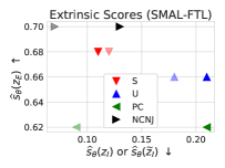
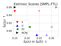
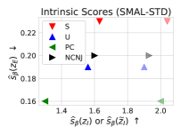
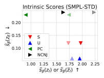
Figure 22: Pose-aware retrieval scores with the STD AE model. Model notation refers to the GDVAE++ model with (S) or without (U) rotation supervision, use of the PC-derived LBOS (PC; see §5.3.3), and the partial disentanglement loss ablation (NCNJ; see §5.3.4). The lighter (partially transparent) counterparts of each point corresponds to using $\widetilde{z}_{I}$ instead of $z_{I}$ for retrieval. We reproduce the FTL AE plots (from Fig. 19) to aid in comparison. See also Appendix Table 6 for detailed values. Compared to the FTL case, for SMPL, U performs relatively better on intrinsic scores, while S and U are relatively similar for extrinsic scores. For SMAL, we see that the extrinsic scores are generally better with the STD AE, compared to the FTL one. We also see that, in the STD case, the PCLBO scenario performs relatively better on SMAL than its S/U counterparts. Finally, we note that using the spectrum-derived latents $\widetilde{z}_{I}$ are generally better, but not always (e.g., on SMPL-STD).

Appendix F Implementation Details

All models were implemented in Pytorch (Paszke et al., 2019). Notationally, let $n=\text{dim}(x_{c})$, $n_{E}=\text{dim}(z_{E})$, $n_{I}=\text{dim}(z_{I})$, and $n_{R}=\text{dim}(z_{R})$. For this section, we assume that the number of points $N_{p}$ in a point cloud (PC) is the same for inputs and outputs (though the architectures themselves do not require this). Validation sets of size 40 (or 250 for MNIST) were set aside from the training set to observe generalization error estimates. Hyper-parameters were largely set based on qualitative examination of training outputs.

F.1 Autoencoder Details

F.1.1 AE Network Architectures

Both the STD and FTL architectures used the same network components, with slight hyper-parameter alterations. Our encoders $E_{r}:\mathbb{R}^{3N_{p}}\rightarrow\mathbb{R}^{4}$ and $E_{x}:\mathbb{R}^{3N_{p}}\rightarrow\mathbb{R}^{n}$ were implemented as PointNets (Qi et al., 2017) without spatial transformers, with hidden channel sizes (64,128,256,512,128) and (128,256,512,836,1024). The inputs are only the point coordinates (i.e., three channels) and the output is a four-dimensional quaternion for $E_{r}$ and an $n$-dimensional vector for $E_{x}$. The decoder $D:\mathbb{R}^{n}\rightarrow\mathbb{R}^{3N_{p}}$ is implemented as a fully connected network, with hidden layer sizes (K,2K,4K), where $K=1200$ for STD and $K=1250$ for FTL. Within $D$, each layer consisted of a linear layer, layer normalization (Ba et al., 2016), and ReLU (except for the last, which had only a linear layer). For the MNIST dataset only, we changed the hidden layer sizes of the decoder $D$ to be (512,1024,1536).

F.1.2 AE Hyper-Parameters and Loss Weights

For architectural parameters, in the FTL case, we set $N_{s}=333$, and hence $n=999$. For STD, we let $n=600$ and did not notice improvements when increasing it. For MNIST, we set $N_{s}=32$ and, for the STD case, $n=150$. Regarding loss parameters, we set the reconstruction loss weights to $\alpha_{C}=200$, $\alpha_{H}=1$, $\widetilde{\gamma}_{P}=100$, and $\gamma_{P}=20$, in the FTL case, altering only $\gamma_{P}=250$ in the STD case. Rotational consistency and prediction loss weights were set to $\gamma_{c}=1$ and $\gamma_{r}=10$. Regularization loss weights were $\gamma_{w}=\gamma_{d}=2\times 10^{-5}$. For MNIST, we altered $\gamma_{c}=50$ for STD, while we let $\gamma_{d}=10^{-6}$, $\gamma_{w}=5\times 10^{-5}$, and $\gamma_{c}=100$ for FTL.

F.1.3 AE Training Details

We train all AEs with Adam (Kingma and Ba, 2014), using an initial learning rate of 0.0005. For supervised AEs, we pretrain the rotation predictor for 2000 iterations before the rest of the network. We use a scheduler that decreases the learning rate by 5% upon hitting a loss plateau, until it reaches 0.0001. We trained MNIST, SMAL, SMPL, and HA for 200, 1250, 350, and 400 epochs, respectively, and batch sizes of 64/100 (FTL/STD) and 36/40 for MNIST and non-MNIST datasets. We set the number of rotated copies (which expands the batch sizes above) to $N_{R}=3$, except in the case of MNIST (for which we used $N_{R}=6$ in the FTL case and $N_{R}=4$ in the STD case). Finally, note that, during training, for the supervised case only, we replace the predicted rotation $\widehat{R}$ with the real one $R$ in all operations.

F.2 Variational Autoencoder Details

For implementation of the HFVAE, we use ProbTorch (Narayanaswamy et al., 2017). Our normalizing flow subnetwork used nflows (Durkan et al., 2020).

F.2.1 VAE Network Architectures

For the VAE, all networks except for the flow mapping $f_{\lambda}$ are implemented as fully connected networks (linear-layernorm-ReLU, as above). Approximate variational posteriors have diagonal covariances. Thus, we have the following mappings with their hidden sizes:

• The rotation distribution parameter encoders, $\mu_{R}:\mathbb{R}^{4}\rightarrow\mathbb{R}^{n_{R}}$ and $\Sigma_{R}:\mathbb{R}^{4}\rightarrow\mathbb{R}^{n_{R}}$, are implemented with an initial shared network, with hidden sizes (256, 128) into an intermediate dimensionality of 64, followed by single linear layer each.

• The quaternion decoder $D_{q}:\mathbb{R}^{n_{R}}\rightarrow\mathbb{R}^{4}$ is structured as (64, 128, 256).

• The intrinsic and extrinsic parameter encoders, $\mu_{\xi}:\mathbb{R}^{n}\rightarrow\mathbb{R}^{n_{\xi}}$ and $\Sigma_{\xi}:\mathbb{R}^{n}\rightarrow\mathbb{R}^{n_{\xi}}$, for $\xi\in\{E,I\}$, have identical network architectures across latent group types: (2000,1600,1200,400) and (2000,1200,400), for $\mu_{\xi}$ and $\Sigma_{\xi}$, respectively.

• The only mapping that is not a fully connected network is the bijective flow $f_{\lambda}$ (and its inverse, $g_{\lambda}$). Recall that we use $f_{\lambda}$ as $\widetilde{\mu}$. Hence, $f_{\lambda}:\mathbb{R}^{N_{\lambda}}\rightarrow\mathbb{R}^{n_{I}}$ and $N_{\lambda}=n_{I}$. This is implemented as a normalizing flow with nine layers, where each layer consists of an affine coupling transform (Dinh et al., 2016), an activation normalization (actnorm) (Kingma and Dhariwal, 2018), and a random feature ordering permutation. The last layer does not have normalization or permutation. Each affine coupling uses an internal FC network with one hidden layer of size 400.

• For the GDVAE++  training regime, we require a covariance parameter estimator for inference during training: $\Sigma_{\xi}:\mathbb{R}^{N_{\lambda}}\rightarrow\mathbb{R}^{n_{I}}$. This is implemented via hidden layers (2n_I, 2n_I).

• The shape decoder $D_{x}:\mathbb{R}^{n_{I}+n_{E}}\rightarrow\mathbb{R}^{n}$ is an FC network with hidden layers (600,1200,1600,2000).

F.2.2 VAE Hyper-Parameters and Loss Weights

Recall that the loss hyper-parameters control the following terms: the intra-group total correlation (TC) $\beta_{1}$, dimension-wise KL divergence $\beta_{2}$, mutual information $\beta_{3}$, inter-group TC $\beta_{4}$, log-likelihood reconstruction $\omega_{R}$, relative quaternion reconstruction $\omega_{q}$, flow likelihood $\omega_{p}$, intrinsics consistency in $z_{I}$-space $\omega_{I}$, intrinsics consistency in $\lambda$-space $\omega_{\lambda}$, covariance disentanglement $\omega_{\Sigma}$, and Jacobian disentanglement $\omega_{\mathcal{J}}$.

Table 7: VAE hyper-parameters across datasets. These values are for the GDVAE++   training method. See text in Appendix §F.2.2 for details.

	$\beta_{2}$	$\beta_{4}$	$\omega_{R}$	$\omega_{\Sigma}$	$\omega_{I}$	$\omega_{\lambda}$	$n_{E}$	$n_{I}$
MNIST	50	100	350	80	600	0	4	24
SMAL	10	50	400	40	300	200	8	24
SMPL	20	100	350	80	600	0	12	20
HA	20	80	360	60	450	100	10	22

In all cases, we set $n_{R}=3$, $\beta_{1}=1$, $\beta_{3}=1$, $\omega_{p}=1$, $\omega_{\mathcal{J}}=200$, and $\omega_{q}=10$. See Table 7 for dataset-dependent parameters. An additional $L_{2}$ weight decay was applied to all networks, with a strength of $10^{-4}$. For the flow-only (GDVAE-FO) approach, the parameters are the same per dataset, except for $\omega_{I}$ and $\omega_{\lambda}$ (which were tuned more in line with original GDVAE model, in an effort to improve disentanglement). For the FO case, we set $\omega_{\lambda}=800$ and $\omega_{I}$ to 0, 250, and 0, for SMAL, SMPL and HA, respectively.

F.2.3 VAE Training Details

As in the AE case, optimization is done with Adam, using a reduce-on-plateau scheduler. The initial learning rate was set to 0.0001, with a minimum of 0.00001. A batch size of 264 was used, except for MNIST, for which we used 512. The networks were trained for 25000 iterations for MNIST and 40000 iterations for all other datasets. We note that for the GDVAE++  mode only, we also cut the gradient of the $\omega_{I}$ loss term from flowing through $\widetilde{\mu}_{I}$ (preventing extrinsic information in $\mu_{I}$ from contaminating $\widetilde{\mu}_{I}$).

Appendix G Full Rotation-Space Experiments

Table 8: AE evaluation on held-out test data with full 3D rotations. Metrics (left to right) refer to the Chamfer distance in reconstructions and the rotational consistency measures (in 3D and $x_{c}$-space, respectively); see §5.2. We place the scores obtained by the corresponding single-axis models in square brackets beside each value (from Table 1), for ease of comparison. Notice the deterioration in both reconstruction and rotation invariance, compared to the single axis case. Nevertheless, note that (1) $\mathcal{C}_{\text{3D}}$ is of a smaller magnitude than $d_{C}(P,\widehat{P})$, suggesting the presence of some rotation invariance, and (2) $\mathcal{C}_{X}$ are larger than zero (the expected value if there were no latent structure in the space).

Dataset	Model	$d_{C}(P,\widehat{P})\downarrow$	$\mathcal{C}_{\text{3D}}\downarrow$	$\mathcal{C}_{X}\uparrow$
SMAL	FTL-S	0.46 [0.10]	0.41 [0.14]	0.11 [0.93]
	FTL-U	0.29 [0.10]	1.32 [0.21]	0.17 [0.88]

We also provide some limited tests our method on full 3D rotations, rather than single-axis rotations. We find that the invariance properties are severely reduced in this more difficult scenario. In particular, we train two AEs on SMAL, both using the FTL architecture and allowing arbitrary rotations. We try both the supervised (S) and unsupervised (U) cases.

Results are shown in Table 8. We see that both reconstruction and rotation invariance are worsened; however, note that (1) $\mathcal{C}_{\text{3D}}$ is of a smaller magnitude than $d_{C}(P,\widehat{P})$ (for S), suggesting the presence of some rotation invariance, and (2) $\mathcal{C}_{X}$ are larger than zero (the expected value if there were no latent structure in the space). Corroborating this latter point, in Fig. 23, we can qualitatively see that the tight latent clustering of rotated objects (as in Fig. 11) is no longer present, but that there is still some structure in the space, by which same-identity objects stay nearby under rotation.

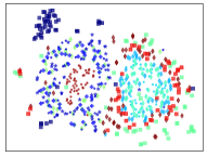
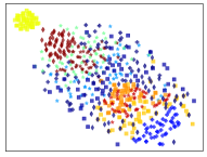
Figure 23: Qualitative visualization of latent AE space with respect to full 3D rotation. Similar to Fig. 11, we show a t-SNE of the latent embeddings of random shapes under random rotations (we show more rotations as the set of rotations is now much larger). Heuristically, we can see there is some clustering structure in the space, but it does not have the tight invariance of the single-axis case. We show the supervised (S) case on the left and unsupervised (U) case on the right. See §G for additional details.

We utilized slightly different hyper-parameters compared to the standard AE case. In particular, for S, we set the batch size to $B=3$ and $N_{R}=48$ trained for 24 epochs; for U, we set $B=2$ and $N_{R}=60$. Decoder layers were set via $K=1400$ (see §F.1). Loss weights were modified to $\gamma_{c}=8000$, $\widetilde{\gamma}_{P}=50/7$, $\gamma_{P}=10/7$ (S case) and $\gamma_{c}=500$, $\widetilde{\gamma}_{P}=400/7$, $\gamma_{P}=80/7$ (U case), to compensate for the larger rotational space.

Appendix H Mesh Experiments

H.1 AMASS Experiments

H.1.1 AE Settings

Following other works (e.g., Marin et al. (2021); Tan et al. (2018)), we use a fully connected AE for the AMASS meshes. In particular, the encoder and decoder have hidden layers (1024,512) and (512,1024). A latent dimension of $\dim(x)=128$ was used. Both networks use the SELU activation (Klambauer et al., 2017) and no normalization. Note that AMASS shapes use the SMPL mesh, with $N_{\text{SMPL}}=6890$ nodes.

The loss utilized for training modifies only $\mathcal{L}_{P}$, which (in the FTL case) is given by

$$\mathcal{L}_{P}=\gamma_{P}D_{V}(V,\widehat{V}),$$ (20)

where $D_{V}(V_{1},V_{2})$ is the vertex-to-vertex mean squared error between the input nodal coordinate sets. Other loss terms remain the same as in the PC case. We set $\gamma_{P}=5$ and use weight decay with $\gamma_{w}=10^{-3}$. For simplicity, following Zhou et al. (2020), we include the global rotation in $z_{E}$ rather than using a separate latent variable. Note that the input and output size is much larger for AMASS than for the PC case (6890 vs. 1600 points). The same learning setup was used as in the PC case, except we apply AdamW (Loshchilov and Hutter, 2017) with a learning rate of $10^{-4}$ and batch size of 100. We run for 250 epochs, using the same train, validation, and test splits as USPD. Notice that, while the AE uses the identical meshing of the input for the reconstruction loss, it does not perform any disentanglement. The VAE, which does perform disentanglement, uses only the raw $x$ values (and does not update the AE), without correspondence or label information.

H.1.2 VAE Settings

We slightly modify the architecture of the VAE, removing batch normalization and replacing ReLU with SELU (as in the AE). We also increase the layer sizes: the flow network is given 10 layers, the encoders that predict $\mu_{E}$ and $\mu_{I}$ use hidden layers (2400,2000,1600,800), and the decoder uses (2000,1800, 1600, 800) for hidden layers; other networks are unchanged. We then use following hyper-parameters, with the SMPL (PC) settings as the default unless otherwise mentioned $\omega_{R}=750$, $\beta_{2}=5$, $\beta_{4}=500$, $\omega_{\Sigma}=5$ $\omega_{\mathcal{J}}=50$, $\omega_{I}=\omega_{\lambda}=1000$, $n_{E}=18$, and $n_{I}=9$. No weight decay was used. We trained with a batch size of 2200 for 40K iterations, starting from initial learning rate $5\times 10^{-5}$.

H.1.3 Empirical Variation

We also compute variabilities on our mesh experiments (see §5.4.1), to give an indication of the variability in the results for our method. For pose transfers, we obtain a standard deviation of 8.08. Table 9 shows the standard errors of the mean for the pose-aware retrieval task. In general, the standard deviations are fairly high. However, following USPD, the held-out data sets from AMASS are of size 10,733 for pose transfer and 11,738 for retrieval, meaning the standard error of the mean is relatively small.

Table 9: Pose-aware retrieval standard errors of the mean on mesh data from AMASS. Data is shown as mean plus/minus standard error (with means from Table 3). Note that our latent intrinsics and extrinsics nomenclature refers to the latent “shape” and “pose” (or articulation) vectors in other works. See §H.1.3 for additional details.

Retrieval with latent:		Intrinsics	Extrinsics
GDVAE++	$\widetilde{E}_{\beta}\pm\sigma(\widetilde{E}_{\beta})$	0.41 $\pm$ 0.0162	1.36 $\pm$ 0.0272
	$\widetilde{E}_{\theta}\pm\sigma(\widetilde{E}_{\theta})$	1.15 $\pm$ 0.0065	0.80 $\pm$ 0.0066
GDVAE++	$\widetilde{E}_{\beta}\pm\sigma(\widetilde{E}_{\beta})$	0.50 $\pm$ 0.0179	1.49 $\pm$ 0.0282
(PCA)	$\widetilde{E}_{\theta}\pm\sigma(\widetilde{E}_{\theta})$	1.21 $\pm$ 0.0065	0.82 $\pm$ 0.0067

H.2 CoMA Experiments

H.2.1 Dataset

We use the same data as in Marin et al. (2021), namely 1853 training meshes with 100 faces from an unseen subject for the shape-from-spectrum recovery test set. We also use their data and dimensionality for the LBOS eigenvalues, so we set $\dim(\lambda)=30$, and treat the meshes at full resolution (3931 vertices and 7800 faces).

H.2.2 AE settings

Following Marin et al. (2021), we use the same fully connected AE to derive the initial latent representation $x$: tanh was used as the non-linearity, no normalization was applied, and the hidden layers were given by (300,200,30,200) (with input and output in $\mathbb{R}^{3|V|}$), with $\dim(x)=30$. The reconstruction loss was the vertex-to-vertex MSE, with weight $\gamma_{P}=5$. We set the weight decay to $\gamma_{w}=0.01$, the radial regularization to $\gamma_{d}=0$, and the batch size to 16. Since this dataset has no orientation changes, we fix our rotation prediction to be identity.

H.2.3 VAE settings

We use the same VAE architecture as the PC experiments. Only the hyper-parameters and training settings are altered, which we leave at the SMPL settings by default, except for the following changes (see also §F.2.2 for details): $\omega_{R}=250$, $\beta_{2}=5$, $\beta_{4}=250$, $\omega_{\Sigma}=100$ $\omega_{\mathcal{J}}=250$, $\omega_{I}=\omega_{\lambda}=1000$, $n_{E}=1$, and $n_{I}=30$. A lighter weight decay of $10^{-6}$ was used. We trained with a batch size of 720 for 30K iterations, starting from initial learning rate $5\times 10^{-5}$. While this setup works well for the shape-from-spectrum task (see Table 4), and it mimics the $\dim(\lambda)=30$ setting from Marin et al. (2021), we found qualitatively that disentangled interpolations could be improved by altering these settings to $n_{E}=4$, $n_{I}=12$, $\omega_{R}=50$, and $\beta_{4}=\omega_{J}=500$, which we use for Fig. 21. This is likely due to facial deformations not being exactly isometric; hence, using too high LBOS dimensionality (and too low $\dim(z_{E})$) leads to $z_{I}$ capturing information we might not expect to be intrinsic (but improving shape-from-spectrum performance).

References

- Achlioptas et al. (2017) Achlioptas P, Diamanti O, Mitliagkas I, Guibas L (2017) Learning representations and generative models for 3D point clouds. arXiv preprint arXiv:170702392
- Andreux et al. (2014) Andreux M, Rodola E, Aubry M, Cremers D (2014) Anisotropic Laplace-Beltrami operators for shape analysis. In: ECCV
- Aubry et al. (2011) Aubry M, Schlickewei U, Cremers D (2011) The wave kernel signature: A quantum mechanical approach to shape analysis. In: ICCV Workshops
- Aumentado-Armstrong et al. (2019) Aumentado-Armstrong T, Tsogkas S, Jepson A, Dickinson S (2019) Geometric disentanglement for generative latent shape models. In: ICCV
- Ba et al. (2016) Ba JL, Kiros JR, Hinton GE (2016) Layer normalization. arXiv preprint arXiv:160706450
- Baek et al. (2015) Baek SY, Lim J, Lee K (2015) Isometric shape interpolation. Computers & Graphics 46:257–263
- Basset et al. (2020) Basset J, Wuhrer S, Boyer E, Multon F (2020) Contact preserving shape transfer: Retargeting motion from one shape to another. Computers & Graphics
- Bengio et al. (2013) Bengio Y, Courville A, Vincent P (2013) Representation learning: A review and new perspectives. IEEE transactions on pattern analysis and machine intelligence 35(8):1798–1828
- Berkiten et al. (2017) Berkiten S, Halber M, Solomon J, Ma C, Li H, Rusinkiewicz S (2017) Learning detail transfer based on geometric features. In: Computer Graphics Forum
- Boscaini et al. (2015a) Boscaini D, Eynard D, Kourounis D, Bronstein MM (2015a) Shape-from-operator: Recovering shapes from intrinsic operators. In: Computer Graphics Forum
- Boscaini et al. (2015b) Boscaini D, Masci J, Melzi S, Bronstein MM, Castellani U, Vandergheynst P (2015b) Learning class-specific descriptors for deformable shapes using localized spectral convolutional networks. In: Computer Graphics Forum
- Bronstein et al. (2011) Bronstein AM, Bronstein MM, Guibas LJ, Ovsjanikov M (2011) Shape google: Geometric words and expressions for invariant shape retrieval. ACM Transactions on Graphics (TOG) 30(1):1
- Chen et al. (2019a) Chen C, Li G, Xu R, Chen T, Wang M, Lin L (2019a) Clusternet: Deep hierarchical cluster network with rigorously rotation-invariant representation for point cloud analysis. In: CVPR
- Chen et al. (2019b) Chen X, Chen B, Mitra NJ (2019b) Unpaired point cloud completion on real scans using adversarial training. arXiv preprint arXiv:190400069
- Chen et al. (2019c) Chen X, Lin KY, Liu W, Qian C, Lin L (2019c) Weakly-supervised discovery of geometry-aware representation for 3D human pose estimation. In: CVPR
- Chen et al. (2019d) Chen X, Song J, Hilliges O (2019d) Monocular neural image based rendering with continuous view control. In: ICCV
- Chern et al. (2018) Chern A, Knöppel F, Pinkall U, Schröder P (2018) Shape from metric. ACM Transactions on Graphics (TOG) 37(4):1–17
- Choukroun et al. (2018) Choukroun Y, Shtern A, Bronstein AM, Kimmel R (2018) Hamiltonian operator for spectral shape analysis. IEEE transactions on visualization and computer graphics
- Chu and Golub (2005) Chu M, Golub G (2005) Inverse eigenvalue problems: theory, algorithms, and applications. OUP Oxford
- Chua and Jarvis (1997) Chua CS, Jarvis R (1997) Point signatures: A new representation for 3D object recognition. International Journal of Computer Vision 25(1):63–85
- Cohen et al. (2018) Cohen TS, Geiger M, Köhler J, Welling M (2018) Spherical cnns. arXiv preprint arXiv:180110130
- Corman et al. (2017) Corman E, Solomon J, Ben-Chen M, Guibas L, Ovsjanikov M (2017) Functional characterization of intrinsic and extrinsic geometry. ACM Transactions on Graphics (TOG) 36(2):14
- Cosmo et al. (2019) Cosmo L, Panine M, Rampini A, Ovsjanikov M, Bronstein MM, Rodolà E (2019) Isospectralization, or how to hear shape, style, and correspondence. In: CVPR
- Cosmo et al. (2020) Cosmo L, Norelli A, Halimi O, Kimmel R, Rodolà E (2020) Limp: Learning latent shape representations with metric preservation priors. arXiv preprint arXiv:200312283
- Dinh et al. (2014) Dinh L, Krueger D, Bengio Y (2014) NICE: Non-linear independent components estimation. arXiv preprint arXiv:14108516
- Dinh et al. (2016) Dinh L, Sohl-Dickstein J, Bengio S (2016) Density estimation using real NVP. arXiv preprint arXiv:160508803
- Durkan et al. (2020) Durkan C, Bekasov A, Murray I, Papamakarios G (2020) nflows: normalizing flows in PyTorch. Zenodo DOI 10.5281/zenodo.4296287, URL https://doi.org/10.5281/zenodo.4296287
- Dym and Maron (2020) Dym N, Maron H (2020) On the universality of rotation equivariant point cloud networks. arXiv preprint arXiv:201002449
- Esmaeili et al. (2018) Esmaeili B, Wu H, Jain S, Bozkurt A, Siddharth N, Paige B, Brooks DH, Dy J, van de Meent JW (2018) Structured disentangled representations. arXiv preprint arXiv:180402086
- Fuchs et al. (2020) Fuchs FB, Worrall DE, Fischer V, Welling M (2020) SE(3)-transformers: 3D roto-translation equivariant attention networks. arXiv preprint arXiv:200610503
- Fumero et al. (2021) Fumero M, Cosmo L, Melzi S, Rodolà E (2021) Learning disentangled representations via product manifold projection. In: ICML
- Gao et al. (2018) Gao L, Yang J, Qiao YL, Lai YK, Rosin PL, Xu W, Xia S (2018) Automatic unpaired shape deformation transfer. ACM Transactions on Graphics (TOG) 37(6):1–15
- Gebal et al. (2009) Gebal K, Bærentzen JA, Aanæs H, Larsen R (2009) Shape analysis using the auto diffusion function. In: Computer Graphics Forum
- Ghosh et al. (2019) Ghosh P, Sajjadi MS, Vergari A, Black M, Schölkopf B (2019) From variational to deterministic autoencoders. arXiv preprint arXiv:190312436
- Gordon et al. (1992) Gordon C, Webb DL, Wolpert S (1992) One cannot hear the shape of a drum. Bulletin of the American Mathematical Society 27(1):134–138
- Groueix et al. (2018) Groueix T, Fisher M, Kim VG, Russell BC, Aubry M (2018) 3D-CODED: 3D correspondences by deep deformation. In: ECCV
- Guo et al. (2014) Guo Y, Bennamoun M, Sohel F, Lu M, Wan J (2014) 3D object recognition in cluttered scenes with local surface features: a survey. IEEE Transactions on Pattern Analysis and Machine Intelligence 36(11):2270–2287
- Higgins et al. (2017) Higgins I, Matthey L, Pal A, Burgess C, Glorot X, Botvinick M, Mohamed S, Lerchner A (2017) -VAE: Learning basic visual concepts with a constrained variational framework. In: ICLR
- Huang et al. (2019) Huang R, Rakotosaona MJ, Achlioptas P, Guibas LJ, Ovsjanikov M (2019) Operatornet: Recovering 3D shapes from difference operators. In: ICCV
- Huynh (2009) Huynh DQ (2009) Metrics for 3D rotations: Comparison and analysis. Journal of Mathematical Imaging and Vision 35(2):155–164
- Johnson and Hebert (1999) Johnson AE, Hebert M (1999) Using spin images for efficient object recognition in cluttered 3D scenes. IEEE Transactions on pattern analysis and machine intelligence 21(5):433–449
- Kac (1966) Kac M (1966) Can one hear the shape of a drum? The american mathematical monthly 73(4P2):1–23
- Kingma and Ba (2014) Kingma DP, Ba J (2014) Adam: A method for stochastic optimization. arXiv preprint arXiv:14126980
- Kingma and Dhariwal (2018) Kingma DP, Dhariwal P (2018) Glow: Generative flow with invertible 1x1 convolutions. In: NeurIPS
- Kingma et al. (2016) Kingma DP, Salimans T, Jozefowicz R, Chen X, Sutskever I, Welling M (2016) Improved variational inference with inverse autoregressive flow. NeurIPS
- Klambauer et al. (2017) Klambauer G, Unterthiner T, Mayr A, Hochreiter S (2017) Self-normalizing neural networks. NeurIPS
- Kobyzev et al. (2020) Kobyzev I, Prince S, Brubaker M (2020) Normalizing flows: An introduction and review of current methods. IEEE Transactions on Pattern Analysis and Machine Intelligence
- Kondor et al. (2018) Kondor R, Son HT, Pan H, Anderson B, Trivedi S (2018) Covariant compositional networks for learning graphs. arXiv preprint arXiv:180102144
- Kovnatsky et al. (2013) Kovnatsky A, Bronstein MM, Bronstein AM, Glashoff K, Kimmel R (2013) Coupled quasi-harmonic bases. In: Computer Graphics Forum
- Kumar et al. (2017) Kumar A, Sattigeri P, Balakrishnan A (2017) Variational inference of disentangled latent concepts from unlabeled observations. arXiv preprint arXiv:171100848
- LeCun et al. (1998) LeCun Y, Bottou L, Bengio Y, Haffner P (1998) Gradient-based learning applied to document recognition. Proceedings of the IEEE 86(11):2278–2324
- Levinson et al. (2019) Levinson J, Sud A, Makadia A (2019) Latent feature disentanglement for 3D meshes. arXiv preprint arXiv:190603281
- Lévy (2006) Lévy B (2006) Laplace-Beltrami eigenfunctions: towards an algorithm that understands geometry. In: Shape Modeling and Applications, 2006. SMI 2006. IEEE International Conference on, IEEE, pp 13–13
- Li et al. (2019) Li J, Bi Y, Lee GH (2019) Discrete rotation equivariance for point cloud recognition. In: ICRA
- Liu et al. (2017) Liu HTD, Jacobson A, Crane K (2017) A Dirac operator for extrinsic shape analysis. In: Computer Graphics Forum
- Loper et al. (2015) Loper M, Mahmood N, Romero J, Pons-Moll G, Black MJ (2015) SMPL: A skinned multi-person linear model. ACM Trans Graphics (Proc SIGGRAPH Asia) 34(6):248:1–248:16
- Loshchilov and Hutter (2017) Loshchilov I, Hutter F (2017) Decoupled weight decay regularization. arXiv preprint arXiv:171105101
- van der Maaten and Hinton (2008) van der Maaten L, Hinton G (2008) Visualizing data using t-sne. Journal of machine learning research 9(Nov):2579–2605
- MacQueen et al. (1967) MacQueen J, et al. (1967) Some methods for classification and analysis of multivariate observations. In: Proceedings of the fifth Berkeley symposium on mathematical statistics and probability, Oakland, CA, USA
- Mahmood et al. (2019) Mahmood N, Ghorbani N, Troje NF, Pons-Moll G, Black MJ (2019) AMASS: Archive of motion capture as surface shapes. In: ICCV
- Marin et al. (2020) Marin R, Rampini A, Castellani U, Rodola E, Ovsjanikov M, Melzi S (2020) Instant recovery of shape from spectrum via latent space connections. In: 2020 International Conference on 3D Vision (3DV), IEEE, pp 120–129
- Marin et al. (2021) Marin R, Rampini A, Castellani U, Rodolà E, Ovsjanikov M, Melzi S (2021) Spectral shape recovery and analysis via data-driven connections. International Journal of Computer Vision pp 1–16
- Masoumi and Hamza (2017) Masoumi M, Hamza AB (2017) Spectral shape classification: A deep learning approach. Journal of Visual Communication and Image Representation 43:198–211
- Melzi et al. (2018) Melzi S, Rodolà E, Castellani U, Bronstein MM (2018) Localized manifold harmonics for spectral shape analysis. In: Computer Graphics Forum
- Meyer et al. (2003) Meyer M, Desbrun M, Schröder P, Barr AH (2003) Discrete differential-geometry operators for triangulated 2-manifolds. In: Visualization and mathematics III, Springer, pp 35–57
- Moschella et al. (2022) Moschella L, Melzi S, Cosmo L, Maggioli F, Litany O, Ovsjanikov M, Guibas L, Rodolà E (2022) Learning spectral unions of partial deformable 3D shapes. In: Computer Graphics Forum
- Narayanaswamy et al. (2017) Narayanaswamy S, Paige B, Van de Meent JW, Desmaison A, Goodman N, Kohli P, Wood F, Torr P (2017) Learning disentangled representations with semi-supervised deep generative models. In: NeurIPS
- Neumann et al. (2014) Neumann T, Varanasi K, Theobalt C, Magnor M, Wacker M (2014) Compressed manifold modes for mesh processing. In: Computer Graphics Forum
- Ovsjanikov et al. (2012) Ovsjanikov M, Ben-Chen M, Solomon J, Butscher A, Guibas L (2012) Functional maps: a flexible representation of maps between shapes. ACM Transactions on Graphics (TOG) 31(4):1–11
- Panine and Kempf (2016) Panine M, Kempf A (2016) Towards spectral geometric methods for euclidean quantum gravity. Physical Review D 93(8):084033
- Papamakarios et al. (2019) Papamakarios G, Nalisnick E, Rezende DJ, Mohamed S, Lakshminarayanan B (2019) Normalizing flows for probabilistic modeling and inference. arXiv preprint arXiv:191202762
- Paszke et al. (2019) Paszke A, Gross S, Massa F, Lerer A, Bradbury J, Chanan G, Killeen T, Lin Z, Gimelshein N, Antiga L, Desmaison A, Kopf A, Yang E, DeVito Z, Raison M, Tejani A, Chilamkurthy S, Steiner B, Fang L, Bai J, Chintala S (2019) Pytorch: An imperative style, high-performance deep learning library. NeurIPS
- Patané (2016) Patané G (2016) Star-laplacian spectral kernels and distances for geometry processing and shape analysis. In: Computer Graphics Forum
- Pedregosa et al. (2012) Pedregosa F, Varoquaux G, Gramfort A, Michel V, Thirion B, Grisel O, Blondel M, Prettenhofer P, Weiss R, Dubourg V, VanderPlas J, Passos A, Cournapeau D, Brucher M, Perrot M, Duchesnay E (2012) Scikit-learn: Machine learning in python. CoRR abs/1201.0490, URL http://arxiv.org/abs/1201.0490, 1201.0490
- Pons-Moll et al. (2015) Pons-Moll G, Romero J, Mahmood N, Black MJ (2015) Dyna: A model of dynamic human shape in motion. ACM Transactions on Graphics, (Proc SIGGRAPH) 34(4):120:1–120:14
- Poulenard et al. (2019) Poulenard A, Rakotosaona MJ, Ponty Y, Ovsjanikov M (2019) Effective rotation-invariant point cnn with spherical harmonics kernels. arXiv preprint arXiv:190611555
- Qi et al. (2017) Qi CR, Su H, Mo K, Guibas LJ (2017) Pointnet: Deep learning on point sets for 3D classification and segmentation. CVPR
- Rampini et al. (2021) Rampini A, Pestarini F, Cosmo L, Melzi S, Rodola E (2021) Universal spectral adversarial attacks for deformable shapes. In: CVPR
- Ranjan et al. (2018) Ranjan A, Bolkart T, Sanyal S, Black MJ (2018) Generating 3D faces using convolutional mesh autoencoders. In: ECCV
- Remelli et al. (2020) Remelli E, Han S, Honari S, Fua P, Wang R (2020) Lightweight multi-view 3D pose estimation through camera-disentangled representation. In: CVPR
- Reuter (2010) Reuter M (2010) Hierarchical shape segmentation and registration via topological features of Laplace-Beltrami eigenfunctions. International Journal of Computer Vision 89(2-3):287–308
- Reuter et al. (2006) Reuter M, Wolter FE, Peinecke N (2006) Laplace–Beltrami spectra as Shape-DNA of surfaces and solids. Computer-Aided Design 38(4):342–366
- Rhodin et al. (2018) Rhodin H, Salzmann M, Fua P (2018) Unsupervised geometry-aware representation for 3D human pose estimation. In: ECCV
- Rhodin et al. (2019) Rhodin H, Constantin V, Katircioglu I, Salzmann M, Fua P (2019) Neural scene decomposition for multi-person motion capture. In: CVPR
- Roberts et al. (2020) Roberts RA, dos Anjos RK, Maejima A, Anjyo K (2020) Deformation transfer survey. Computers & Graphics
- Rodolà et al. (2017) Rodolà E, Cosmo L, Bronstein MM, Torsello A, Cremers D (2017) Partial functional correspondence. In: Computer Graphics Forum
- Rustamov (2007) Rustamov RM (2007) Laplace-Beltrami eigenfunctions for deformation invariant shape representation. In: Proceedings of the fifth Eurographics symposium on Geometry processing, Eurographics Association, pp 225–233
- Sanghi (2020) Sanghi A (2020) Info3D: Representation learning on 3D objects using mutual information maximization and contrastive learning. arXiv preprint arXiv:200602598
- Sanghi and Danielyan (2019) Sanghi A, Danielyan A (2019) Towards 3D rotation invariant embeddings. CVPR 2019 Workshop on 3D Scene Understanding for Vision, Graphics, and Robotics
- Sharp and Crane (2020) Sharp N, Crane K (2020) A Laplacian for nonmanifold triangle meshes. In: Computer Graphics Forum
- Sharp et al. (2021) Sharp N, Gillespie M, Crane K (2021) Geometry processing with intrinsic triangulations. SIGGRAPH’21: ACM SIGGRAPH 2021 Courses
- Shoemake (1985) Shoemake K (1985) Animating rotation with quaternion curves. In: Proceedings of the 12th annual conference on Computer graphics and interactive techniques, pp 245–254
- Stein et al. (1992) Stein F, Medioni G, et al. (1992) Structural indexing: Efficient 3-D object recognition. IEEE Transactions on Pattern Analysis and Machine Intelligence 14(2):125–145
- Su et al. (2021) Su FG, Lin CS, Wang YCF (2021) Learning interpretable representation for 3D point clouds. In: ICPR, IEEE
- Sumner and Popović (2004) Sumner RW, Popović J (2004) Deformation transfer for triangle meshes. ACM Transactions on graphics (TOG) 23(3):399–405
- Sun et al. (2009) Sun J, Ovsjanikov M, Guibas L (2009) A concise and provably informative multi-scale signature based on heat diffusion. In: Computer Graphics Forum
- Sun et al. (2019) Sun X, Lian Z, Xiao J (2019) SRINet: Learning strictly rotation-invariant representations for point cloud classification and segmentation. In: Proceedings of the 27th ACM International Conference on Multimedia, pp 980–988
- Tan et al. (2018) Tan Q, Gao L, Lai YK, Xia S (2018) Variational autoencoders for deforming 3D mesh models. In: CVPR
- Taubin (1995) Taubin G (1995) A signal processing approach to fair surface design. In: Proceedings of the 22nd annual conference on Computer graphics and interactive techniques, pp 351–358
- Thomas et al. (2018) Thomas N, Smidt T, Kearnes S, Yang L, Li L, Kohlhoff K, Riley P (2018) Tensor field networks: Rotation-and translation-equivariant neural networks for 3D point clouds. arXiv preprint arXiv:180208219
- Tombari et al. (2010) Tombari F, Salti S, Di Stefano L (2010) Unique signatures of histograms for local surface description. In: ECCV
- Vallet and Lévy (2008) Vallet B, Lévy B (2008) Spectral geometry processing with manifold harmonics. In: Computer Graphics Forum
- Varol et al. (2017) Varol G, Romero J, Martin X, Mahmood N, Black MJ, Laptev I, Schmid C (2017) Learning from synthetic humans. In: CVPR
- Vinh et al. (2010) Vinh NX, Epps J, Bailey J (2010) Information theoretic measures for clusterings comparison: Variants, properties, normalization and correction for chance. The Journal of Machine Learning Research 11:2837–2854
- Wang et al. (2017) Wang Y, Ben-Chen M, Polterovich I, Solomon J (2017) Steklov spectral geometry for extrinsic shape analysis. arXiv preprint arXiv:170707070
- Watanabe (1960) Watanabe S (1960) Information theoretical analysis of multivariate correlation. IBM Journal of research and development 4(1):66–82
- Weyl (1911) Weyl H (1911) Über die asymptotische verteilung der eigenwerte. Nachrichten von der Gesellschaft der Wissenschaften zu Göttingen, Mathematisch-Physikalische Klasse 1911:110–117
- Worrall and Brostow (2018) Worrall D, Brostow G (2018) CubeNet: Equivariance to 3D rotation and translation. In: ECCV
- Worrall et al. (2017) Worrall DE, Garbin SJ, Turmukhambetov D, Brostow GJ (2017) Interpretable transformations with encoder-decoder networks. In: ICCV
- Xiao et al. (2020) Xiao Z, Lin H, Li R, Geng L, Chao H, Ding S (2020) Endowing deep 3D models with rotation invariance based on principal component analysis. In: 2020 IEEE International Conference on Multimedia and Expo (ICME)
- Yang et al. (2019) Yang G, Huang X, Hao Z, Liu MY, Belongie S, Hariharan B (2019) PointFlow: 3D point cloud generation with continuous normalizing flows. arXiv preprint arXiv:190612320
- Ye et al. (2018) Ye Z, Diamanti O, Tang C, Guibas L, Hoffmann T (2018) A unified discrete framework for intrinsic and extrinsic Dirac operators for geometry processing. In: Computer Graphics Forum
- Yin et al. (2015) Yin M, Li G, Lu H, Ouyang Y, Zhang Z, Xian C (2015) Spectral pose transfer. Computer Aided Geometric Design 35:82–94
- You et al. (2018) You Y, Lou Y, Liu Q, Tai YW, Ma L, Lu C, Wang W (2018) Pointwise rotation-invariant network with adaptive sampling and 3D spherical voxel convolution. arXiv preprint arXiv:181109361
- Zhang et al. (2020) Zhang X, Qin S, Xu Y, Xu H (2020) Quaternion product units for deep learning on 3D rotation groups. In: CVPR
- Zhang et al. (2019) Zhang Z, Hua BS, Rosen DW, Yeung SK (2019) Rotation invariant convolutions for 3D point clouds deep learning. In: International Conference on 3D Vision (3DV)
- Zhao et al. (2020) Zhao Y, Birdal T, Lenssen JE, Menegatti E, Guibas L, Tombari F (2020) Quaternion equivariant capsule networks for 3D point clouds. In: ECCV
- Zhou et al. (2020) Zhou K, Bhatnagar BL, Pons-Moll G (2020) Unsupervised shape and pose disentanglement for 3D meshes. In: ECCV
- Zuffi et al. (2017) Zuffi S, Kanazawa A, Jacobs D, Black MJ (2017) 3D menagerie: Modeling the 3D shape and pose of animals. In: CVPR