Structural Characterization of Oscillations in Brain Networks with Rate Dynamics

Abstract

Among the versatile forms of dynamical patterns of activity exhibited by the brain, oscillations are one of the most salient and extensively studied, yet are still far from being well understood. In this paper, we provide various structural characterizations of the existence of oscillatory behavior in neural networks using a classical neural mass model of mesoscale brain activity called linear-threshold dynamics. Exploiting the switched-affine nature of this dynamics, we obtain various necessary and/or sufficient conditions on the network structure and its external input for the existence of oscillations in (i) two-dimensional excitatory-inhibitory networks (E-I pairs), (ii) networks with one inhibitory but arbitrary number of excitatory nodes, (iii) purely inhibitory networks with an arbitrary number of nodes, and (iv) networks of E-I pairs. Throughout our treatment, and given the arbitrary dimensionality of the considered dynamics, we rely on the lack of stable equilibria as a system-based proxy for the existence of oscillations, and provide extensive numerical results to support its tight relationship with the more standard, signal-based definition of oscillations in computational neuroscience.

1 Introduction

Oscillations are among some of the first forms of neuronal activity to be discovered in the human brain, thanks particularly to the invention of electroencephalogram (EEG) nearly a century ago [3]. Thanks to their conceptual simplicity, prominence, and unmistakable correlation with various neurocognitive processes, oscillations have since been the subject of significant research from experimental and computational perspectives in neuroscience [9, 58, 30, 20, 13, 44]. Nevertheless, the precise mechanisms by which oscillations are generated are still not understood. In this work, we seek to shed light on this challenging problem using an analytical, system-theoretic approach and the linear-threshold mean-field model of neuronal dynamics. Our results constitute some of the first rigorous characterizations of the existence of oscillations in these networks, spanning various network architectures from simple, two-dimensional networks to arbitrarily complex interconnections of them.

Literature Review: Oscillations have been the subject of extensive research in the neuroscience literature, see, e.g. [9, 58, 30, 20, 13, 44], often from solely experimental and/or numerical perspectives. In comparison, analytical characterizations of oscillations have remained far behind, even though they can enable a more precise understanding of the role that different network components and their interconnections have in the appearance of oscillations, with potential implications for the study of abnormal behavior (e.g., epilepsy, Parkinson), information transmission, medical interventions, and beyond. Among analytical studies, the Wilson-Cowan model [61] has played a special role owing to its minimal architecture and richness of non-trivial dynamics at the same time. Nevertheless, analytical characterization of structural conditions giving rise to oscillations even in the Wilson-Cowan model has not moved beyond partial results [2, 4, 38, 43], mainly due to the intractability of the sigmoidal nonlinearity in the standard model. This has motivated the study of variants of the sigmoidal activation function, such as linear-threshold models. Analytical results have been developed in [11] for the Wilson-Cowan model with bounded linear-threshold activation functions, but only under a number of unrealistic assumptions (notably, the violation of Dale’s law, excluding interaction terms inside the nonlinear activation functions, and a chain network topology). Similar to neural mass models with sigmoidal nonlinearities, models with linear-threshold activation functions also exhibit rich nonlinear phenomena including multistability, limit cycles, chaos, and bifurcations, see e.g., [39, 12]. In our previous work, we characterized the existence and uniqueness of equilibria and asymptotic stability in linear-threshold networks with arbitrary topologies [42] and also provided sufficient and necessary conditions for the existence of oscillations in two-dimensional excitatory-inhibitory networks and their networked excitatory-coupled interconnection [41]. Among other contributions, the present work extends this characterization to the existence of oscillations in excitatory-inhibitory networks with arbitrary number of excitatory nodes and networks of two-dimensional oscillators with more realistic, excitatory-to-all inter-oscillator connections.

Oscillations have also been studied extensively using bifurcation theory (particularly the Hopf bifurcation), see e.g., [29, 19, 59, 6, 43, 22, 49, 51] and references therein. However, a fundamental limitation of these works, and a major difference with the approach here, is the univariate nature of the former. In other words, bifurcation analysis is often conducted by fixing all (of the numerous) network parameters and studying the effect of varying one or two parameters at a time. In contrast, our global analysis provides a complete characterization of the set of all parameters that give rise to oscillations, a set whose boundaries consist of bifurcation points. Significant research has been conducted, in the controls and neuroscience communities alike, to characterize oscillatory dynamics using models of phase oscillators, the most notable of which being the Kuramoto model, see [5, 37] and references therein. However, while the Kuramoto model has the advantage of having a smaller (half) state dimension, it is only a valid approximation to the Wilson-Cowan model in the weakly coupled regime [50, 25], where interconnected oscillators primarily affect each other’s phase dynamics and their amplitude dynamics can be neglected. Moving beyond the weakly connected regime, amplitude dynamics, particularly saturations and phase-amplitude coupling [26, 43], become critical [18] and more complex models, such as the full Wilson-Cowan model are required.

Statement of Contributions: Our main contributions are fourfold, and consist of conditions on the structure of linear-threshold networks and their inputs that are necessary and/or sufficient to guarantee the lack of stable equilibria (LoSE). Since conditions for the existence of limit cycles in systems with higher than two dimensions are unknown in general, we use LoSE (which constitutes the main condition in the Poincaré-Bendixson theory for existence of limit cycles in planar systems) as a proxy for the existence of oscillations. First, motivated by the higher abundance and versatility of excitatory neurons in the mammalian cortex, we provide a necessary and sufficient condition for LoSE in networks with a single inhibitory but arbitrary excitatory nodes. We also describe two important consequences of this result, including a simple, intuitive, and exact characterization of limit cycles in the Wilson-Cowan model with linear-threshold nonlinearity, as well as the fact that purely excitatory networks always have stable equilibria. Second, purely inhibitory networks have long been known to be able to generate oscillations, and are often believed to play a central role in cortical oscillations in the brain. Our second contribution consists of an extensive study of LoSE in such networks, where we provide structural necessary conditions on the synaptic connectivity matrix for LoSE for arbitrary inhibitory networks and a full characterization of LoSE for pairwise unstable ones. For the latter case, we provide a graph-theoretic interpretation for the existence of inputs that induce oscillations in terms of the presence of special cycles we term valid in the complete graph whose weights are defined in terms of the synaptic weight matrix. Next, we study oscillations in networks of multiple brain regions, each modeled by a simple Wilson-Cowan oscillator. Our third contribution consists of exact, necessary and sufficient conditions for LoSE in such networks, when they are coupled either only through their excitatory nodes or via both excitatory-to-excitatory and excitatory-to-inhibitory connections. Finally, we provide extensive numerical evidence that LoSE is indeed a near necessary and sufficient system-based proxy for the existence of oscillations, where the latter is often defined based on the power spectral density of the system’s trajectories. Together, our results provide the first rigorous characterization of the existence of oscillations in linear-threshold networks with several different classes of network architectures, along with the introduction of a novel proxy for oscillatory systems, whose relevance is of independent interest for the study of arbitrary dynamical systems.

2 Problem Formulation

Consider a neuronal network composed of a large number of neurons that communicate via sequences of spikes. Grouping together neurons with similar firing rates, under standard assumptions (see, e.g., [15, Ch 7]), the mean-field dynamics of the network can be described by the linear-threshold model

$$\tau\dot{\mathbf{x}}(t)=-\mathbf{x}(t)+[\mathbf{W}\mathbf{x}(t)+\mathbf{u}]_{\mathbf{0}}^{\mathbf{m}},\qquad\mathbf{x}(0)\in[\mathbf{0},\mathbf{m}],$$ (1)

where $\mathbf{x}\in^{N}$ is the state vector with $x_{i}$ denoting the average firing rate of the $i$’th neuronal population, $\mathbf{W}\in^{N\times N}$ is the matrix of average synaptic connectivities, $\mathbf{u}\in^{N}$ is the vector of average external (background) inputs to the populations, $\mathbf{m}\in\mathbb{R}_{>0}^{N}$ is the vector of average maximum firing rates, and $\tau>0$ is the network time constant. Note that all solutions are bounded as $[\mathbf{0},\mathbf{m}]$ is invariant under (1).

Our previous work [42] characterized the existence and uniqueness of equilibria and asymptotic stability for a variant of (1) with unbounded activation function ($\mathbf{m}=\infty\cdot\mathbf{1}_{N}$), and these results are readily extensible to arbitrary finite $\mathbf{m}$. However, the existence of oscillations in linear-threshold dynamics is not as well understood. Further, brain networks often contain interconnections of multiple coupled oscillators, and our understanding is even smaller about the oscillatory behavior of interconnections of (1). Our goal is to characterize the relationship between network structure and the oscillatory behavior observed in linear-threshold dynamics modeling brain networks.

Problem 1.

We seek to answer the following questions for the bounded linear-threshold network dynamics (1):

1. What are neural oscillations? That is, what is an objective definition of oscillatory signals and oscillatory systems?

2. What network structures give rise to oscillations?

3. What are the structural conditions for the existence of oscillations in networked interconnections of multiple oscillatory networks?

Following common practice in computational neuroscience [10, 17], we here adopt a broad notion of oscillations that includes both periodic oscillations (limit cycles) and chaotic ones. In the latter case, a chaotic behavior is oscillatory if its state trajectories are near-periodic, as captured by next.

Definition 2.1.

(Oscillation). A state trajectory $\mathbf{x}(t),t\geq 0$ of (1) is oscillatory if

1. its power spectrum contains distinct and pronounced resonance peaks; and

2. it does not asymptotically converge to a constant limit. $\square$

Two remarks about Definition 2.1 are in order. First, property (i) is qualitative and fuzzy in nature, as is the notion of oscillation. Different measures can be used to quantify this property, such as the regularity index $\chi_{\rm reg}$, cf. Appendix A. Second, the property (ii) is included in the definition of an oscillation to limit our focus to sustained (a.k.a. persistent) oscillations and not transient ones. It is important to note that both types of oscillations are observed in neuronal dynamics (see, e.g., [9, 53, 34, 46] for sustained and [32, 57] for transient), albeit with potentially different underlying dynamical generators. Our focus here is on the former category in light of the vast literature on attractor dynamics in biological neuronal networks [28, 36, 33, 56], while the latter remains an avenue for future research.

The analytical tools in the study of oscillations are generally limited to 2-dimensional systems (cf. the Poincaré-Bendixson theory [45, Ch 3]) or higher-dimensional systems that are essentially confined to 2-dimensional manifolds (see, e.g., [21, 48]). Thus, throughout the paper, we use lack of stable equilibria (LoSE) as a proxy for oscillations. In fact, this condition constitutes the main requirement in the Poincaré-Bendixson theory for existence of limit cycles. In Appendix A, we show numerically that this proxy is a tight characterization of oscillatory dynamics for the model (1).

To study the equilibria of (1), we use its representation as a switched affine system [35, 31]. It is straightforward to show [42] that ^N can be decomposed into $3^{N}$ switching regions $\{\Omega_{\boldsymbol{\sigma}}\}_{{\boldsymbol{\sigma}}\in\{0,\ell,{\rm s}\}^{N}}$ defined by

$$\mathbf{x}\in\Omega_{\boldsymbol{\sigma}}\Leftrightarrow\begin{cases}(\mathbf{W}\mathbf{x}+\mathbf{u})_{i}\in(-\infty,0];&\forall i\ \ {\rm s.t.}\ \ \sigma_{i}=0,\\ (\mathbf{W}\mathbf{x}+\mathbf{u})_{i}\in[0,m_{i}];&\forall i\ \ {\rm s.t.}\ \ \sigma_{i}=\ell,\\ (\mathbf{W}\mathbf{x}+\mathbf{u})_{i}\in[m_{i},\infty);&\forall i\ \ {\rm s.t.}\ \ \sigma_{i}={\rm s},\end{cases}$$

where $0$, $\ell$, and ${\rm s}$ denote a node in inactive, active (linear), and saturated state, respectively. Thus, (1) can be rewritten in the switched affine form

$$\tau\dot{\mathbf{x}}=(-\mathbf{I}+\boldsymbol{\Sigma}^{\ell}\mathbf{W})\mathbf{x}+\boldsymbol{\Sigma}^{\ell}\mathbf{u}+\boldsymbol{\Sigma}^{\rm s}\mathbf{m},\qquad\forall\mathbf{x}\in\Omega_{\boldsymbol{\sigma}},$$ (2)

where for any ${\boldsymbol{\sigma}}\in\{0,\ell,{\rm s}\}^{N}$, $\boldsymbol{\Sigma}^{\ell}\in^{N\times N}$ and $\boldsymbol{\Sigma}^{\rm s}\in^{N\times N}$ are diagonal matrices with entries

$$\Sigma_{ii}^{\ell}=\begin{cases}1&\text{if }\sigma_{i}=\ell,\\ 0&\text{if }\sigma_{i}=0,{\rm s},\end{cases}\qquad\Sigma_{ii}^{\rm s}=\begin{cases}1&\text{if }\sigma_{i}={\rm s},\\ 0&\text{if }\sigma_{i}=0,\ell.\end{cases}$$

Each $\Omega_{\boldsymbol{\sigma}}$ then has a corresponding equilibrium candidate

$$\mathbf{x}^{*}_{\boldsymbol{\sigma}}=(\mathbf{I}-\boldsymbol{\Sigma}^{\ell}\mathbf{W})^{-1}(\boldsymbol{\Sigma}^{\ell}\mathbf{u}+\boldsymbol{\Sigma}^{\rm s}\mathbf{m}),$$ (3)

and the equilibria of (1) consist of all equilibrium candidates $\mathbf{x}^{*}_{\boldsymbol{\sigma}}$ that belong to their respective switching regions. Note, in particular, that while the position of the equilibrium candidates depend on all four of $\mathbf{W}$, $\mathbf{u}$, $\mathbf{m}$, and ${\boldsymbol{\sigma}}$, their stability is a sole function of $\mathbf{W}$ and ${\boldsymbol{\sigma}}$.

In what follows, we derive exact as well as simplified characterizations of LoSE for networks with various (and increasingly more complex) architectures. The network architectures that we study respect an important property of mammalian cortical networks, known as Dale’s law [61, 15], according to which each node has either an excitatory or inhibitory effect on other nodes, but not both. This means that each column of $\mathbf{W}$ is either nonnegative or nonpositive, a condition that we follow throughout the paper.

3 Oscillations in Single Networks

We analyze the dynamics (1) and derive conditions on the network $(\mathbf{W},\mathbf{u},\mathbf{m})$ giving rise to oscillatory behavior.

3.1 Excitatory-Inhibitory Networks

The reciprocal interactions between excitatory and inhibitory populations of cortical neurons have long been known to be a major contributor to cortical oscillations [30]. Arguably, the simplest scenario with only one excitatory and one inhibitory populations (each abstracted to one network node) has been the most popular in theoretical neuroscience [14]. Interestingly, this coincides with the fact that LoSE is, under mild conditions, necessary and sufficient for the existence of almost globally (excluding trajectories starting at an unstable equilibrium) asymptotically stable limit cycles when $N=2$. This two-dimensional case, hereafter called an E-I pair, is the celebrated Wilson-Cowan model used in computational neuroscience for decades [61, 2, 4, 38, 43]. Unlike the standard model with sigmoidal activation functions, however, the next result shows that a complete characterization of limit cycles can be obtained for Wilson-Cowan models with bounded linear-threshold nonlinearities.

Theorem 3.1.

(Limit cycles in E-I pairs). Consider the dynamics (1) with $N=2$ and

$$\mathbf{W}=\begin{bmatrix}a&-b\\ c&-d\end{bmatrix},\qquad a,b,c,d\geq 0.$$

All network trajectories (except those starting at an unstable equilibrium, if any) converge to a limit cycle if and only if

$$d+2 <a,$$ (4a)

$$(a-1)(d+1) <bc,$$ (4b)

$$(a-1)m_{1} <bm_{2},$$ (4c)

$$0<u_{1} <bm_{2}-(a-1)m_{1},$$ (4d)

$$0<(d+1)u_{1}-bu_{2} <\big{[}bc-(a-1)(d+1)\big{]}m_{1}.$$ (4e)

By [52, Thm 4.1], all the trajectories (except those starting at unstable equilibria, if any) converge to a limit cycle if and only if the network does not have any stable equilibria. This is, nevertheless, not a special case of Theorem 3.2 as we here do not presume (4a) but rather show its necessity together with (4b)-(4e).

If $a<1$, then all the regions $\Omega_{\boldsymbol{\sigma}},{\boldsymbol{\sigma}}\in\{0,\ell,{\rm s}\}^{2}$ are stable, ensuring the existence of a stable equilibrium (since the existence of an equilibrium is always guaranteed by the Brouwer fixed point theorem [7]). Thus, assume $a\geq 1$. Then, as shown in the proof of Theorem 3.2, the trivially stable regions $(\sigma^{\prime},j),\sigma^{\prime}\in\{0,{\rm s}\},j\in\{0,\ell,{\rm s}\}$ do not contain their equilibrium candidates iff $u\in Y^{c}$. One can readily show

$$Y =\Big{\{}(u_{1},u_{2})\;|\;u_{1}\leq\max\big{\{}0,\min\{bm_{2},\frac{b}{d+1}u_{2}\}\big{\}}\ \text{or}$$

$$u_{1}\geq-(a-1)m_{1}+\min\big{\{}bm_{2},\max\{0,\frac{b(u_{2}+cm_{1})}{d+1}\}\big{\}}\Big{\}}.$$

Therefore, $u\in Y^{c}$ if and only if

$$u_{1} >0,$$ (5a)

$$u_{1} <bm_{2}-(a-1)m_{1},$$ (5b)

$$u_{1} >\min\{bm_{2},\frac{b}{d+1}u_{2}\},$$ (5c)

$$u_{1} <-(a-1)m_{1}+\max\{0,\frac{b(u_{2}+cm_{1})}{d+1}\}.$$ (5d)

For (5) to be feasible, it is necessary and sufficient that

$$\text{\eqref{eq:yca} and~{}\eqref{eq:ycb} :}\ bm_{2}-(a-1)m_{1}>0,$$ (6a)

$$\text{\eqref{eq:yca} and~{}\eqref{eq:ycd} :}\ u_{2}>-\frac{bc-(a-1)(d+1)}{b}m_{1},$$ (6b)

$$\text{\eqref{eq:ycb} and~{}\eqref{eq:ycc} :}\ u_{2}<\frac{d+1}{b}(bm_{2}-(a-1)m_{1}),$$ (6c)

$$\text{\eqref{eq:ycc} and~{}\eqref{eq:ycd} :}\ bc>(a-1)(d+1).$$ (6d)

Conditions (6a) and (6d) are the same as (4c) and (4b), respectively. Furthermore, under (6), (5) simplifies to (4d) and (4e), which in turn ensure (6b) and (6c). In conclusion, $u\in Y^{c}$ if and only if (4b)-(4e) hold.

What remains to study are the regions $(\ell,0)$, $(\ell,{\rm s})$, and $(\ell,\ell)$. The first two are not stable since $a\geq 1$. Also, though not needed, they do not include their equilibrium candidates due to (4d). On the other hand, for ${\boldsymbol{\sigma}}=(\ell,\ell)$,

$$\mathbf{x}^{*}_{\boldsymbol{\sigma}}=\frac{1}{bc-(a-1)(d+1)}\begin{bmatrix}(d+1)u_{1}-bu_{2}\\ cu_{1}-(a-1)u_{2}\end{bmatrix}=\mathbf{W}\mathbf{x}^{*}_{\boldsymbol{\sigma}}+\mathbf{u}.$$

The first component of $\mathbf{W}\mathbf{x}^{*}_{\boldsymbol{\sigma}}+\mathbf{u}$ clearly belongs to $[0,m_{1}]$ by (4b) and (4e). For its second component, we have

$$\eqref{eq:eib},\eqref{eq:eie} \Rightarrow cu_{1}>(a-1)u_{2},$$

$$\eqref{eq:eid},\eqref{eq:eie} \Rightarrow u_{2}>\frac{c}{a-1}u_{1}-\frac{bc-(a-1)(d+1)}{a-1}m_{2},$$

ensuring that ${\boldsymbol{\sigma}}=(\ell,\ell)$ always contains its equilibrium candidate. Therefore, this region must be unstable which, under (4b), happens if and only if $a>d+2$. ∎

While the simplicity of this two-dimensional E-I model has led to its long-standing popularity in the computational neuroscience literature, it clearly comes at the price of limited flexibility to model the complex dynamics of the brain. In the rest of this paper, we extend the above analysis to more complex scenarios, beginning with the following analysis of higher-dimensional excitatory-inhibitory networks.

Inhibitory neurons constitute about $20\%$ of neurons in the cortex and have broader (less specific) interconnection and activity patterns than excitatory neurons. Therefore, we focus on networks with a single inhibitory node and arbitrary number of excitatory nodes. Let $N=n+1$, $n\geq 1$, and consider

$$\mathbf{W}=\begin{bmatrix}\mathbf{a}&-\mathbf{b}\\ \mathbf{c}&-d\end{bmatrix},\quad\mathbf{u}=\begin{bmatrix}\mathbf{u}_{e}\\ u_{n+1}\end{bmatrix},\quad\mathbf{m}=\begin{bmatrix}\mathbf{m}_{e}\\ m_{n+1}\end{bmatrix},$$ (7)

where $\mathbf{a}\in\mathbb{R}_{\geq 0}^{n\times n}$, $\mathbf{b}\in\mathbb{R}_{\geq 0}^{n\times 1}$, $\mathbf{c}\in\mathbb{R}_{\geq 0}^{1\times n}$, $d\in\mathbb{R}_{\geq 0}$. Note that this class of networks includes, as a special case, the well-known 2-dimensional Wilson-Cowan model ($n=1$) extensively used in the computational neuroscience [16].We are ready to give our first result on LoSE for (1)-(7).

Theorem 3.2.

(Networks with a single inhibitory node). Consider the dynamics (1), (7) and assume that

$$a_{ii}>d+2\qquad\forall i\in\{1,\dots,n\}.$$ (8)

Then, the network does not have any stable equilibria iff $\mathbf{u}\in^{n+1}\setminus Y$, where

$$Y =\bigcup\nolimits_{{\boldsymbol{\sigma}}^{\prime}\in\{0,{\rm s}\}^{n}}\bigg{[}\bigcap\nolimits_{i\in{\boldsymbol{\sigma}}^{\prime}}\!\left(Y_{{\boldsymbol{\sigma}}^{\prime},{\rm s},i}\cup(Y_{{\boldsymbol{\sigma}}^{\prime},0,i}\cap Y_{{\boldsymbol{\sigma}}^{\prime},\ell,i})\right)\cap$$

$$\hskip 69.0pt\bigcap\nolimits_{i\notin{\boldsymbol{\sigma}}^{\prime}}\!\left(Y_{{\boldsymbol{\sigma}}^{\prime},0,i}\cup(Y_{{\boldsymbol{\sigma}}^{\prime},{\rm s},i}\cap Y_{{\boldsymbol{\sigma}}^{\prime},\ell,i})\right)\bigg{]},$$

$$Y_{{\boldsymbol{\sigma}}^{\prime}\!,j,i} =\begin{cases}\{\mathbf{u}\;|\;u_{i}\geq y_{{\boldsymbol{\sigma}}^{\prime}\!,j,i}\}\ ;&\text{\rm if}\ i\in{\boldsymbol{\sigma}}^{\prime}\\ \{\mathbf{u}\;|\;u_{i}\leq y_{{\boldsymbol{\sigma}}^{\prime}\!,j,i}\}\ ;&\text{\rm if}\ i\notin{\boldsymbol{\sigma}}^{\prime}\end{cases}\quad\forall j\in\{0,\ell,{\rm s}\},$$

$y_{{\boldsymbol{\sigma}}^{\prime}\!,0,i}=-(\mathbf{a}_{i{\boldsymbol{\sigma}}^{\prime}}\!-\!\mathbf{I}_{i{\boldsymbol{\sigma}}^{\prime}})\mathbf{m}_{{\boldsymbol{\sigma}}^{\prime}}$, $y_{{\boldsymbol{\sigma}}^{\prime}\!,{\rm s},i}=y_{{\boldsymbol{\sigma}}^{\prime}\!,0,i}+b_{i}m_{n+1}$, and $y_{{\boldsymbol{\sigma}}^{\prime}\!,\ell,i}=y_{{\boldsymbol{\sigma}}^{\prime}\!,0,i}+\frac{b_{i}(u_{n+1}+\mathbf{c}_{{\boldsymbol{\sigma}}^{\prime}}\mathbf{m}_{{\boldsymbol{\sigma}}^{\prime}})}{d+1}$ for ${\boldsymbol{\sigma}}^{\prime}\in\{0,s\}^{n}$ and $i\in\{1,\dots,n\}$.

The proof consists of two steps: first, we determine the list of $\Omega_{\boldsymbol{\sigma}}$ that are stable and second, we ensure that they do not contain their equilibrium candidates iff $\mathbf{u}\in^{n+1}\setminus Y$.

Step 1: The switching regions can be naturally decomposed into two groups: those in which at least one of the excitatory nodes is active and those in which all the excitatory nodes are either inactive or saturated. We next show that these correspond to unstable and stable switching regions, respectively. Consider any ${\boldsymbol{\sigma}}\in\{0,\ell,{\rm s}\}^{N}$ and let $L=\{i\in\{1,\dots,n\}\;|\;\sigma_{i}=\ell\}$ (note that $L$ is independent of $\sigma_{n+1}$). Let $r=|L|$, and let $\boldsymbol{\Pi}$ be the permutation matrix such that $\boldsymbol{\Pi}{\boldsymbol{\sigma}}=(\mathbf{0}_{n-r},\ell,\dots,\ell,\sigma_{n+1})$. The coefficient matrix $-\mathbf{I}+\boldsymbol{\Sigma}\mathbf{W}$ in the region $\Omega_{\boldsymbol{\sigma}}$ then satisfies $\boldsymbol{\Pi}(-\mathbf{I}+\boldsymbol{\Sigma}\mathbf{W})\boldsymbol{\Pi}^{T}=[-\mathbf{I}_{n-r},\mathbf{0};\star,\mathbf{P}]$, where $\mathbf{P}=[-\mathbf{I}_{r}+\mathbf{a}_{L},\star;\star,-1-\Sigma_{n+1,n+1}d]$, $\mathbf{a}_{L}$ is the principal submatrix of $\mathbf{a}$ composed of its rows and columns in $L$, and $\Sigma_{n+1,n+1}$ is the bottom-right element of $\boldsymbol{\Sigma}$. Thus, the eigenvalues of $-\mathbf{I}+\boldsymbol{\Sigma}\mathbf{W}$ consist of $(-1)$ with multiplicity $n-r$ and the eigenvalues of $\mathbf{P}$. Therefore,

• if $r>0$, $\Omega_{\boldsymbol{\sigma}}$ is unstable since $\text{tr}(\mathbf{P})=\sum_{i\in L}(a_{ii}-1)-1-\Sigma_{n+1,n+1}d\geq\sum_{i\in L}(a_{ii}-1)-1-d\stackrel{{\scriptstyle\eqref{eq:agd2}}}{{>}}0$;

• if $r=0$, $\Omega_{\boldsymbol{\sigma}}$ is stable since $P=-1-\Sigma_{n+1,n+1}d<0$.

Step 2: According to Step 1, we only need to ensure that regions $\Omega_{\boldsymbol{\sigma}}$ with $r=0$ do not contain their equilibrium candidates. These regions have the form

$${\boldsymbol{\sigma}}=({\boldsymbol{\sigma}}^{\prime},j),\qquad{\boldsymbol{\sigma}}^{\prime}\in\{0,{\rm s}\}^{n},\ {j}\in\{0,\ell,{\rm s}\}.$$

We consider three cases based on the value of $j$.

1. $j=0$: It is straightforward to verify that

   $$\mathbf{W}\mathbf{x}^{*}_{\boldsymbol{\sigma}}+\mathbf{u}=\begin{bmatrix}\mathbf{a}_{:,{\boldsymbol{\sigma}}^{\prime}}\mathbf{m}_{{\boldsymbol{\sigma}}^{\prime}}+\mathbf{u}_{e}\\ \mathbf{c}_{{\boldsymbol{\sigma}}^{\prime}}\mathbf{m}_{{\boldsymbol{\sigma}}^{\prime}}+u_{n+1}\end{bmatrix},$$

   and that $\mathbf{W}\mathbf{x}^{*}_{\boldsymbol{\sigma}}+\mathbf{u}\in\Omega_{\boldsymbol{\sigma}}$ if and only if $\mathbf{u}\in\bigcap_{i=1}^{n+1}Y_{{\boldsymbol{\sigma}}^{\prime},0,i}$ where $Y_{{\boldsymbol{\sigma}}^{\prime},0,n+1}=\{\mathbf{u}\;|\;u_{n+1}\leq-\mathbf{c}_{{\boldsymbol{\sigma}}^{\prime}}\mathbf{m}_{{\boldsymbol{\sigma}}^{\prime}}\}$.

2. $j={\rm s}$: similarly, it follows that

   $$\mathbf{W}\mathbf{x}^{*}_{\boldsymbol{\sigma}}+\mathbf{u}=\begin{bmatrix}\mathbf{a}_{:,{\boldsymbol{\sigma}}^{\prime}}\mathbf{m}_{{\boldsymbol{\sigma}}^{\prime}}-\mathbf{b}m_{n+1}+\mathbf{u}_{e}\\ \mathbf{c}_{{\boldsymbol{\sigma}}^{\prime}}\mathbf{m}_{{\boldsymbol{\sigma}}^{\prime}}-dm_{n+1}+u_{n+1}\end{bmatrix},$$

   and $\mathbf{W}\mathbf{x}^{*}_{\boldsymbol{\sigma}}+\mathbf{u}\in\Omega_{\boldsymbol{\sigma}}\Leftrightarrow\mathbf{u}\in\bigcap_{i=1}^{n+1}Y_{{\boldsymbol{\sigma}}^{\prime},{\rm s},i}$ where $Y_{{\boldsymbol{\sigma}}^{\prime},{\rm s},n+1}=\{\mathbf{u}\;|\;u_{n+1}\geq(d+1)m_{n+1}-\mathbf{c}_{{\boldsymbol{\sigma}}^{\prime}}\mathbf{m}_{{\boldsymbol{\sigma}}^{\prime}}\}$.

3. $j=\ell$: it also follows similarly that

   $$(d+1)\mathbf{W}\mathbf{x}^{*}_{\boldsymbol{\sigma}}+\mathbf{u}=$$

   $$\begin{bmatrix}(\mathbf{a}_{:,{\boldsymbol{\sigma}}^{\prime}}(d+1)-\mathbf{b}\mathbf{c}_{{\boldsymbol{\sigma}}^{\prime}})\mathbf{m}_{{\boldsymbol{\sigma}}^{\prime}}-\mathbf{b}u_{n+1}+(d+1)\mathbf{u}_{e}\\ \mathbf{c}_{{\boldsymbol{\sigma}}^{\prime}}\mathbf{m}_{{\boldsymbol{\sigma}}^{\prime}}+u_{n+1}\end{bmatrix},$$

   and $\mathbf{W}\mathbf{x}^{*}_{\boldsymbol{\sigma}}+\mathbf{u}\in\Omega_{\boldsymbol{\sigma}}\Leftrightarrow\mathbf{u}\in\bigcap_{i=1}^{n+1}Y_{{\boldsymbol{\sigma}}^{\prime},\ell,i}$ where $Y_{{\boldsymbol{\sigma}}^{\prime},{\rm s},n+1}=\{\mathbf{u}\;|\;-\mathbf{c}_{{\boldsymbol{\sigma}}^{\prime}}\mathbf{m}_{{\boldsymbol{\sigma}}^{\prime}}\leq u_{n+1}\leq(d+1)m_{n+1}-\mathbf{c}_{{\boldsymbol{\sigma}}^{\prime}}\mathbf{m}_{{\boldsymbol{\sigma}}^{\prime}}\}$.

Therefore, for no stable region to contain its equilibrium candidate it is necessary and sufficient that

$$\mathbf{u}\in^{n+1}\setminus\bar{Y},\qquad\bar{Y}=\bigcup_{{\boldsymbol{\sigma}}^{\prime}\in\{0,{\rm s}\}^{n}}\bigcup_{j\in\{0,\ell,{\rm s}\}}\bigcap_{i=1}^{n+1}Y_{{\boldsymbol{\sigma}}^{\prime},j,i}.$$ (9)

It only remains to show $\bar{Y}=Y$. For ${\boldsymbol{\sigma}}^{\prime}\in\{0,{\rm s}\}^{n}$, let

$$\bar{Y}_{{\boldsymbol{\sigma}}^{\prime}}=\bigcup_{j\in\{0,\ell,{\rm s}\}}\bigcap_{i=1}^{n+1}Y_{{\boldsymbol{\sigma}}^{\prime},j,i}.$$ (10)

Then, we have $\bar{Y}_{{\boldsymbol{\sigma}}^{\prime}}^{c}=\bigcap_{j\in\{0,\ell,{\rm s}\}}\bigcup_{i=1}^{n+1}Y_{{\boldsymbol{\sigma}}^{\prime},j,i}^{c}=\bigcap_{j=1}^{5}(A_{j}^{c}\cup B_{j}^{c})$, where (in what follows, ^∘ denotes the interior of a set)

$$A_{1} =\bigcap_{i=1}^{n}\!Y_{{\boldsymbol{\sigma}}^{\prime},0,i}, B_{1}=Y_{{\boldsymbol{\sigma}}^{\prime},0,n+1}^{\circ},$$

$$A_{2} =A_{1}, B_{2}=Y_{{\boldsymbol{\sigma}}^{\prime},0,n+1}\cap Y_{{\boldsymbol{\sigma}}^{\prime},\ell,n+1},$$

$$A_{3} =\bigcap_{i=1}^{n}\!Y_{{\boldsymbol{\sigma}}^{\prime},\ell,i}, B_{3}=Y_{{\boldsymbol{\sigma}}^{\prime},\ell,n+1}^{\circ},$$

$$A_{4} =A_{3}, B_{4}=Y_{{\boldsymbol{\sigma}}^{\prime},\ell,n+1}\cap Y_{{\boldsymbol{\sigma}}^{\prime},{\rm s},n+1},$$

$$A_{5} =\bigcap_{i=1}^{n}\!Y_{{\boldsymbol{\sigma}}^{\prime},{\rm s},i}, B_{5}=Y_{{\boldsymbol{\sigma}}^{\prime},{\rm s},n+1}^{\circ},$$

Since the sets $\{B_{j}\}_{j=1}^{5}$ partition ⁿ⁺¹, it follows that $\bar{Y}_{{\boldsymbol{\sigma}}^{\prime}}^{c}=\bigcup_{j=1}^{5}(A_{j}^{c}\cap B_{j})$, or

$$\bar{Y}_{{\boldsymbol{\sigma}}^{\prime}}^{c} =\bigcup\nolimits_{j\in\{0,\ell,{\rm s}\}}\Big{(}\!\Big{(}\bigcup\nolimits_{i=1}^{n}Y_{{\boldsymbol{\sigma}}^{\prime},j,i}^{c}\Big{)}\cap Y_{{\boldsymbol{\sigma}}^{\prime},j,n+1}\Big{)}$$

$$=\bigcup\nolimits_{i=1}^{n}\bigcup\nolimits_{j\in\{0,\ell,{\rm s}\}}(Y_{{\boldsymbol{\sigma}}^{\prime},j,i}^{c}\cap Y_{{\boldsymbol{\sigma}}^{\prime},j,n+1}).$$ (11)

For any $i\in{\boldsymbol{\sigma}}^{\prime}$, we have

$$\bar{Y}_{{\boldsymbol{\sigma}}^{\prime},i}^{c}\triangleq\bigcup\nolimits_{j\in\{0,\ell,{\rm s}\}}(Y_{{\boldsymbol{\sigma}}^{\prime},j,i}^{c}\cap Y_{{\boldsymbol{\sigma}}^{\prime},j,n+1})$$

$$\stackrel{{\scriptstyle\text{(a)}}}{{=}}\bigcup\nolimits_{j\in\{0,\ell,{\rm s}\}}[(Y_{{\boldsymbol{\sigma}}^{\prime},j,i}^{c}\cap Y_{{\boldsymbol{\sigma}}^{\prime},j,n+1})\cup(Y_{{\boldsymbol{\sigma}}^{\prime},0,i}^{c}\cap Y_{{\boldsymbol{\sigma}}^{\prime},j,n+1})]$$

$$\stackrel{{\scriptstyle\text{(b)}}}{{=}}\bigcup\nolimits_{j\in\{0,\ell,{\rm s}\}}(Y_{{\boldsymbol{\sigma}}^{\prime},j,i}^{c}\cap Y_{{\boldsymbol{\sigma}}^{\prime},j,n+1})\cup Y_{{\boldsymbol{\sigma}}^{\prime},0,i}^{c}$$

$$=Y_{{\boldsymbol{\sigma}}^{\prime},0,i}^{c}\cup(Y_{{\boldsymbol{\sigma}}^{\prime},\ell,i}^{c}\cap Y_{{\boldsymbol{\sigma}}^{\prime},\ell,n+1})\cup(Y_{{\boldsymbol{\sigma}}^{\prime},{\rm s},i}^{c}\cap Y_{{\boldsymbol{\sigma}}^{\prime},{\rm s},n+1})$$

$$\stackrel{{\scriptstyle\text{(c)}}}{{=}}Y_{{\boldsymbol{\sigma}}^{\prime},0,i}^{c}\cup(Y_{{\boldsymbol{\sigma}}^{\prime},\ell,i}^{c}\cap Y_{{\boldsymbol{\sigma}}^{\prime},{\rm s},n+1}^{c})\cup(Y_{{\boldsymbol{\sigma}}^{\prime},{\rm s},i}^{c}\cap Y_{{\boldsymbol{\sigma}}^{\prime},{\rm s},n+1})$$

$$\stackrel{{\scriptstyle\text{(d)}}}{{=}}Y_{{\boldsymbol{\sigma}}^{\prime},0,i}^{c}\cup(Y_{{\boldsymbol{\sigma}}^{\prime},\ell,i}^{c}\cap Y_{{\boldsymbol{\sigma}}^{\prime},{\rm s},n+1}^{c}\cap Y_{{\boldsymbol{\sigma}}^{\prime},{\rm s},i}^{c})$$

$$\qquad\qquad\cup(Y_{{\boldsymbol{\sigma}}^{\prime},{\rm s},i}^{c}\cap Y_{{\boldsymbol{\sigma}}^{\prime},{\rm s},n+1}\cap Y_{{\boldsymbol{\sigma}}^{\prime},\ell,i}^{c})$$

$$=Y_{{\boldsymbol{\sigma}}^{\prime},0,i}^{c}\cup(Y_{{\boldsymbol{\sigma}}^{\prime},\ell,i}^{c}\cap Y_{{\boldsymbol{\sigma}}^{\prime},{\rm s},i}^{c})$$

$$\stackrel{{\scriptstyle\text{(d)}}}{{=}}(Y_{{\boldsymbol{\sigma}}^{\prime},0,i}^{c}\cup Y_{{\boldsymbol{\sigma}}^{\prime},\ell,i}^{c})\cap Y_{{\boldsymbol{\sigma}}^{\prime},{\rm s},i}^{c},$$ (12)

where (a) is because $Y_{{\boldsymbol{\sigma}}^{\prime},0,i}^{c}\cap Y_{{\boldsymbol{\sigma}}^{\prime},j,n+1}\subseteq Y_{{\boldsymbol{\sigma}}^{\prime},j,i}^{c}\cap Y_{{\boldsymbol{\sigma}}^{\prime},j,n+1}$ for both $j=\ell$ and $j={\rm s}$ (and is trivial for $j=0$), (b) is because $\{Y_{{\boldsymbol{\sigma}}^{\prime},j,n+1}\}_{j\in\{0,\ell,{\rm s}\}}$ cover ⁿ⁺¹, (c) is because $Y_{{\boldsymbol{\sigma}}^{\prime},\ell,i}^{c}\cap Y_{{\boldsymbol{\sigma}}^{\prime},\ell,n+1}\subseteq Y_{{\boldsymbol{\sigma}}^{\prime},\ell,i}^{c}\cap Y_{{\boldsymbol{\sigma}}^{\prime},{\rm s},n+1}^{c}$ and

$$(Y_{{\boldsymbol{\sigma}}^{\prime},\ell,i}^{c}\cap Y_{{\boldsymbol{\sigma}}^{\prime},{\rm s},n+1}^{c})\setminus(Y_{{\boldsymbol{\sigma}}^{\prime},\ell,i}^{c}\cap Y_{{\boldsymbol{\sigma}}^{\prime},\ell,n+1})\subseteq Y_{{\boldsymbol{\sigma}}^{\prime},0,i}^{c},$$

(d) is because $Y_{{\boldsymbol{\sigma}}^{\prime},\ell,i}^{c}\cap Y_{{\boldsymbol{\sigma}}^{\prime},{\rm s},n+1}^{c}\subseteq Y_{{\boldsymbol{\sigma}}^{\prime},{\rm s},i}^{c}$ and $Y_{{\boldsymbol{\sigma}}^{\prime},{\rm s},i}^{c}\cap Y_{{\boldsymbol{\sigma}}^{\prime},{\rm s},n+1}\subset Y_{{\boldsymbol{\sigma}}^{\prime},\ell,i}^{c}$, and (e) is because $Y_{{\boldsymbol{\sigma}}^{\prime},0,i}^{c}\subseteq Y_{{\boldsymbol{\sigma}}^{\prime},{\rm s},i}^{c}$. By a parallel argument, it can be shown that for any $i\notin{\boldsymbol{\sigma}}^{\prime}$,

$$\bar{Y}_{{\boldsymbol{\sigma}}^{\prime},i}^{c}=(Y_{{\boldsymbol{\sigma}}^{\prime},{\rm s},i}^{c}\cup Y_{{\boldsymbol{\sigma}}^{\prime},\ell,i}^{c})\cap Y_{{\boldsymbol{\sigma}}^{\prime},0,i}^{c}.$$ (13)

Therefore, (9)-(13) gives $\bar{Y}=Y$, completing the proof. ∎

While the description of $Y$ in Theorem 3.2 may seem complex, it has a simple interpretation. Consider a fixed value for $u_{n+1}$. Then, each of the sets $\left(Y_{{\boldsymbol{\sigma}}^{\prime},{\rm s},i}\cup(Y_{{\boldsymbol{\sigma}}^{\prime},0,i}\cap Y_{{\boldsymbol{\sigma}}^{\prime},\ell,i})\right)$ or $\left(Y_{{\boldsymbol{\sigma}}^{\prime},0,i}\cup(Y_{{\boldsymbol{\sigma}}^{\prime},{\rm s},i}\cap Y_{{\boldsymbol{\sigma}}^{\prime},\ell,i})\right)$ in the definition of $Y$ are a half space of the form $\{u_{i}\geq y\}$ or $\{u_{i}\leq y\}$ (depending on whether $i\in{\boldsymbol{\sigma}}^{\prime}$ or not) that drive $x_{i}$ to saturation or inactivity, respectively. Therefore, the cross section of $Y$ for this fixed value of $u_{n+1}$ is composed of $2^{n}$ closed orthants, each unbounded towards a different direction in ⁿ. Figure 1 shows an example of this for $n=2$. The union of these orthants (the shaded area in Figure 1) characterizes the region where the network has at least one stable equilibrium.

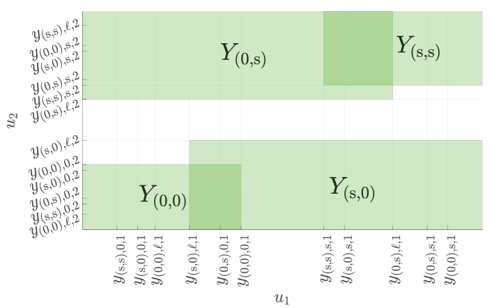
Figure 1: Illustration of the region $Y$ in Theorem 3.2 for an example network with $n=2$. The four shaded quadrants represent the cross section of $Y_{{\boldsymbol{\sigma}}^{\prime}},{\boldsymbol{\sigma}}^{\prime}\in\{0,{\rm s}\}^{2}$ at $u_{3}=-5$, so the white area is where the network lacks any stable equilibria. Network parameters are $\mathbf{a}=[8.5,1;1,5]$, $\mathbf{b}=[5;7]$, $\mathbf{c}=[4,5]$, $d=1$, $\mathbf{m}=[2;3;6]$.

Nevertheless, the set $Y^{c}$ may in general be non-convex, unbounded, and disconnected. The next result gives simpler and easier-to-interpret, but more conservative, conditions.

Corollary 3.3.

(Simpler conditions for networks with a single inhibitory node). Consider the same assumptions as in Theorem 3.2. Then, for the network not to have any stable equilibria, it is necessary that

$$-\mathbf{c}\mathbf{m}_{e}<u_{n+1}<(d+1)m_{n+1},$$ (14)

and sufficient that either

$$0\leq u_{n+1}\leq(d+1)m_{n+1}-\mathbf{c}\mathbf{m}_{e},$$ (15a)

$$\exists i_{0}\ {\rm s.t.}\quad(a_{i_{0}i_{0}}-1)(d+1)<b_{i_{0}}c_{i_{0}},$$ (15b)

$$\frac{b_{i_{0}}u_{n+1}}{d\!+\!1}\!\!<\!u_{i_{0}}\!\!<\!\!\frac{b_{i_{0}}(u_{n+1}\!+\!c_{i_{0}}m_{i_{0}})}{d\!+\!1}\!-\!(a_{i_{0}i_{0}}\!\!-\!1)m_{i_{0}},$$ (15c)

$$u_{i}\!<\!\frac{b_{i}u_{n\!+\!1}\!-\![(\mathbf{a}_{i,:}\!-\!\mathbf{I}_{i,:})(d\!+\!1)\!-\!b_{i}\mathbf{c}]^{+}\mathbf{m}_{e}}{d\!+\!1},\forall i\neq i_{0},$$ (15d)

or

$$(d\!+\!1)m_{n+1}\!-\!\min_{i}(c_{i}m_{i})\!\leq\!u_{n\!+\!1}\leq(d\!+\!1)m_{n+1},$$ (16a)

$$\exists i_{0}\ {\rm s.t.}\quad(a_{i_{0}i_{0}}-1)m_{i_{0}}<b_{i_{0}}m_{n+1},$$ (16b)

$$0<u_{i_{0}}<b_{i_{0}}m_{n+1}-(a_{i_{0}i_{0}}-1)m_{i_{0}},$$ (16c)

$$u_{i}<b_{i}m_{n+1}-(\mathbf{a}_{i,:}-\mathbf{I}_{i,:})\mathbf{m}_{e},\quad\forall i\neq i_{0}.$$ (16d)

First, we prove the sufficiency of the conditions in (15), by showing that any $\mathbf{u}$ satisfying all the conditions in (15) will not belong to $Y$ as defined in Theorem 3.2. Note that the expression for $Y$ can be greatly simplified if we can restrict $\mathbf{u}$ such that for all ${\boldsymbol{\sigma}}^{\prime}\in\{0,{\rm s}\}^{n}$,

$$Y_{{\boldsymbol{\sigma}}^{\prime},{\rm s},i}\cup(Y_{{\boldsymbol{\sigma}}^{\prime},0,i}\cap Y_{{\boldsymbol{\sigma}}^{\prime},\ell,i}) =Y_{{\boldsymbol{\sigma}}^{\prime},\ell,i}\qquad\forall i\in{\boldsymbol{\sigma}}^{\prime},$$

$$Y_{{\boldsymbol{\sigma}}^{\prime},0,i}\cup(Y_{{\boldsymbol{\sigma}}^{\prime},{\rm s},i}\cap Y_{{\boldsymbol{\sigma}}^{\prime},\ell,i}) =Y_{{\boldsymbol{\sigma}}^{\prime},\ell,i}\qquad\forall i\notin{\boldsymbol{\sigma}}^{\prime}$$ (17)

Given the definition of the sets $Y_{{\boldsymbol{\sigma}}^{\prime},j,i}$, we can see that this holds if for all ${\boldsymbol{\sigma}}^{\prime}\in\{0,{\rm s}\}^{n}$,

$$-\mathbf{c}_{{\boldsymbol{\sigma}}^{\prime}}\mathbf{m}_{{\boldsymbol{\sigma}}^{\prime}}\leq u_{n+1}\leq(d+1)m_{n+1}-\mathbf{c}_{{\boldsymbol{\sigma}}^{\prime}}\mathbf{m}_{{\boldsymbol{\sigma}}^{\prime}},$$ (18)

which gives (15a) since $\max_{{\boldsymbol{\sigma}}^{\prime}}-\mathbf{c}_{{\boldsymbol{\sigma}}^{\prime}}\mathbf{m}_{{\boldsymbol{\sigma}}^{\prime}}=0$ and $\min_{{\boldsymbol{\sigma}}^{\prime}}-\mathbf{c}_{{\boldsymbol{\sigma}}^{\prime}}\mathbf{m}_{{\boldsymbol{\sigma}}^{\prime}}=-\mathbf{c}\mathbf{m}_{e}$.

Given (3.1), $\mathbf{u}$ will not be in $Y$ if and only if for any ${\boldsymbol{\sigma}}^{\prime}\in\{0,{\rm s}\}^{n}$, there exists an $i$ such that

$$u_{i}<\frac{b_{i}}{d+1}u_{n+1}+\frac{b_{i}\mathbf{c}_{{\boldsymbol{\sigma}}^{\prime}}-(\mathbf{a}_{i{\boldsymbol{\sigma}}^{\prime}}-\mathbf{I}_{i{\boldsymbol{\sigma}}^{\prime}})(d+1)}{d+1}\mathbf{m}_{{\boldsymbol{\sigma}}^{\prime}},$$ (19a)

if $$i\in{\boldsymbol{\sigma}}^{\prime}$$, or

$$u_{i}>\frac{b_{i}}{d+1}u_{n+1}+\frac{b_{i}\mathbf{c}_{{\boldsymbol{\sigma}}^{\prime}}-(\mathbf{a}_{i{\boldsymbol{\sigma}}^{\prime}}-\mathbf{I}_{i{\boldsymbol{\sigma}}^{\prime}})(d+1)}{d+1}\mathbf{m}_{{\boldsymbol{\sigma}}^{\prime}},$$ (19b)

if $i\notin{\boldsymbol{\sigma}}^{\prime}$. Note that these are $2^{n}$ sets of inequalities, where at least one inequality needs to be satisfied from each set using only the $n$ variables $u_{1},\dots,u_{n}$. This provides us with a choice of which inequality from each set we choose to enforce, with any choice imposing $2^{n}$ upper/lower bounds on $u_{1},\dots,u_{n}$. Here, care should be taken to ensure the resulting system of inequalities is feasible. For any variable $u_{i}$, as long as the inequalities imposed on it are all either lower bounds or upper bounds, a feasible $u_{i}$ exists. However, any lower and upper bounds imposed on the same $u_{i}$ must be ensured to be collectively feasible, in turn putting additional restrictions on $\mathbf{W}$ and $\mathbf{m}$. With this background in mind, we obtain an explicit yet minimally restrictive set of sufficient conditions as follows.

Assume that (15b) holds. Then, we impose the $i$’th inequality corresponding to ${\boldsymbol{\sigma}}^{\prime}=\mathbf{0}$ and ${\boldsymbol{\sigma}}^{\prime}_{i}=(0,0,\dots,{\rm s},\dots,0)$ where the ${\rm s}$ is in the $i$’th position. The result will be (15c), which is feasible by (15b). For any other ${\boldsymbol{\sigma}}^{\prime}\neq\mathbf{0},{\boldsymbol{\sigma}}^{\prime}_{i}$, we only impose some (or all) of the upper bound inequalities in (19a) for $j\neq i$, which will always be feasible without any further restrictions on $\mathbf{W}$ and $\mathbf{m}$. This leads to potentially multiple upper bounds for each $j\neq i$, but all of them are greater than the bound in (15b) and are thus satisfied if (15b) is. This completes the proof of the sufficiency of (15).

Second, we prove the sufficiency of the conditions in (16) following a similar construction. Here, instead of (3.1), we restrict $\mathbf{u}$ such that for all ${\boldsymbol{\sigma}}^{\prime}\neq\mathbf{0}$,

$$Y_{{\boldsymbol{\sigma}}^{\prime},{\rm s},i}\cup(Y_{{\boldsymbol{\sigma}}^{\prime},0,i}\cap Y_{{\boldsymbol{\sigma}}^{\prime},\ell,i}) =Y_{{\boldsymbol{\sigma}}^{\prime},{\rm s},i}\quad\forall i\in\{1,\dots,n\},$$ (20)

and for ${\boldsymbol{\sigma}}^{\prime}=\mathbf{0}$,

$$Y_{{\boldsymbol{\sigma}}^{\prime},{\rm s},i}\cup(Y_{{\boldsymbol{\sigma}}^{\prime},0,i}\cap Y_{{\boldsymbol{\sigma}}^{\prime},\ell,i}) =Y_{{\boldsymbol{\sigma}}^{\prime},0,i}\quad\forall i\in\{1,\dots,n\}.$$ (21)

Similar to (18), these will hold if $-\mathbf{c}_{{\boldsymbol{\sigma}}^{\prime}}\mathbf{m}_{{\boldsymbol{\sigma}}^{\prime}}+(d+1)m_{n+1}\leq u_{n+1}\leq(d+1)m_{n+1}$, for all ${\boldsymbol{\sigma}}^{\prime}\neq\mathbf{0}$, which is equivalent to (16a). Then, similar to the proof of (15), we assume that there exists at least one $i$ for which (16b) holds, and enforce the $i$’th inequality for ${\boldsymbol{\sigma}}^{\prime}=\mathbf{0}$ and ${\boldsymbol{\sigma}}^{\prime}={\boldsymbol{\sigma}}^{\prime}_{i}$. These together impose (16c) on $u_{i}$, whose feasibility requires (16b). For any other ${\boldsymbol{\sigma}}^{\prime}$, we enforce the $j$’th inequality(s) for some (or all) $j\in{\boldsymbol{\sigma}}^{\prime},j\neq i$, which requires $u_{j}<-(\mathbf{a}_{j{\boldsymbol{\sigma}}^{\prime}}-\mathbf{I}_{j{\boldsymbol{\sigma}}^{\prime}})\mathbf{m}_{{\boldsymbol{\sigma}}^{\prime}}+b_{j}m_{n+1}$ and satisfied if the stronger condition (16d) holds.

Finally, we prove the necessity of (14) by contradiction. Assume, first, that $u_{n+1}\geq(d+1)m_{n+1}$. This implies that (20) holds for all ${\boldsymbol{\sigma}}^{\prime}\in\{0,{\rm s}\}^{n}$ and all $i$. We can then make a sequential argument as follows. Starting from ${\boldsymbol{\sigma}}^{\prime}=\mathbf{0}$, we would need at least one $i$ such that $u_{i}>b_{i}m_{n+1}$. This $i$ can then never satisfy $u_{i}<b_{i}m_{n+1}-(\mathbf{a}_{i{\boldsymbol{\sigma}}^{\prime}}-\mathbf{I}_{i{\boldsymbol{\sigma}}^{\prime}})\mathbf{m}_{{\boldsymbol{\sigma}}^{\prime}}$ for any ${\boldsymbol{\sigma}}^{\prime}$, which means that $\mathbf{u}$ cannot belong to any $Y_{{\boldsymbol{\sigma}}^{\prime},{\rm s},i}^{c}$ where $i\in{\boldsymbol{\sigma}}^{\prime}$. To simplify the discussion and without loss of generality, assume we have chosen $i=1$. Then, $\mathbf{u}$ cannot belong to any $Y_{{\boldsymbol{\sigma}}^{\prime},{\rm s},1}^{c}$ for any ${\boldsymbol{\sigma}}^{\prime}=({\rm s},\star,\dots,\star)$. Therefore, for ${\boldsymbol{\sigma}}^{\prime}=({\rm s},0,\dots,0)$, we need at least one $i\geq 2$ such that $u_{i}>b_{i}m_{n+1}-a_{i1}m_{1}$. Again, for simplicity and without loss of generality, assume $i=2$. Then, $\mathbf{u}$ cannot belong to any $Y_{{\boldsymbol{\sigma}}^{\prime},{\rm s},2}^{c}$ for any ${\boldsymbol{\sigma}}^{\prime}=({\rm s},{\rm s},\star,\dots,\star)$. Continuing this argument, we will ultimately have to impose lower bounds on all the elements of $\mathbf{u}_{e}$, which prevent $\mathbf{u}$ from belonging to $Y_{{\boldsymbol{\sigma}}^{\prime},{\rm s},i}^{c}$ for ${\boldsymbol{\sigma}}^{\prime}=({\rm s},{\rm s},\dots,{\rm s})$ and any $i$, ensuring the existence of a stable equilibrium by Theorem 3.2, which is a contradiction. An analogous argument shows that $u_{n+1}\leq-\mathbf{c}\mathbf{m}_{e}$ also leads to a contradiction. ∎

Note the parallelism between (4) and (15)-(16). In fact, conditions (15b), (15c)-(15d), (16b), and (16c)-(16d) are generalizations of (4b), (4e), (4c), and (4d), respectively. Further, Corollary 3.3 has itself a further consequence with great neuroscientific value, as given next.

Corollary 3.4.

(Fully excitatory networks). Given the dynamics (1), if $\mathbf{W}$ is fully excitatory (all entries are non-negative), then the network has at least one stable equilibrium.

A fully excitatory network corresponds to (1), (7) with a sufficiently negative $u_{n+1}$ that drives the inhibitory node into negative saturation, effectively removing it from the network. This happens if, for all $t$, $\mathbf{c}\mathbf{x}_{e}(t)-dx_{n+1}(t)+u_{n+1}<0\Leftarrow u_{n+1}<-\mathbf{c}\mathbf{x}_{e}(t)\Leftarrow u_{n+1}<-\mathbf{c}\mathbf{m}_{e}$, which, by Corollary 3.3, implies at least one stable equilibrium exists. ∎

This result can can also be established using the theory of monotone systems [23, 1]. Corollary 3.4 provides a simple and rigorous explanation for the well-known necessity of inhibitory nodes in brain oscillations [60]. On the other hand, the computational neuroscience literature has long shown the possibility of oscillatory activity in purely inhibitory networks [30], an important class of networks that we treat next.

3.2 Inhibitory Networks

Our focus here is on linear-threshold network models (1) where only inhibitory nodes are present. Consequently,

$$\mathbf{W}=\begin{bmatrix}-d_{1,1}&-d_{1,2}&\dots&-d_{1,N}\\ -d_{2,1}&-d_{2,2}&\dots&-d_{2,N}\\ \vdots&\ddots&\dots&\vdots\\ -d_{N,1}&-d_{N,2}&\dots&-d_{N,N}\end{bmatrix}$$

with $d_{i,j}\geq 0$ for all $i,j$.

3.2.1 Necessary Conditions for LoSE

We start by identifying a necessary condition for the lack of stable equilibria of fully inhibitory networks.

Theorem 3.5.

(Necessary condition for oscillatory behavior in fully inhibitory networks). If a fully inhibitory network does not have any stable equilibria, then $\mathbf{I}-\mathbf{W}\notin\mathbb{P}$.

We argue the counter positive: if $\mathbf{I}-\mathbf{W}\in\mathbb{P}$, then a stable equilibrium point exists. The fact that an equilibrium exists for any $\mathbf{u}\in^{N}$ is a direct consequence of [42, Theorem IV.1]. To show it is stable, let us consider any switching region $\boldsymbol{\Omega}_{\boldsymbol{\sigma}}$ containing the equilibrium. Over this region, the dynamics is described by $-\mathbf{I}+\mathbf{\Sigma}\mathbf{W}$. Let $r$ be the cardinality of the set of nodes in linear state and let $\mathbf{\Pi}$ be a permutation matrix such that $\mathbf{\Pi}\mathbf{\sigma}=(\sigma_{1},\dots,\sigma_{n-r},l,\dots,l)$, where $\sigma_{i}\in\{0,s\}$. Then,

$$\mathbf{\Pi}(-\mathbf{I}+\mathbf{\Sigma}\mathbf{W})\mathbf{\Pi}^{T}=\begin{bmatrix}-\mathbf{I}&0\\ \ast&\mathbf{P}\end{bmatrix},$$ (22)

for some matrix $\mathbf{P}$. The eigenvalues of the system are therefore $-1$, with multiplicity $n-r$, and the eigenvalues of $\mathbf{P}$. Note that $\mathbf{P}$ is a principal submatrix of the matrix $-\mathbf{I}+\mathbf{W}$. Since any principal submatrix of a ${P}-$matrix is also a $P-$matrix, we deduce $-\mathbf{P}$ is a ${P}-$matrix too. In addition, since $\mathbf{W}$ corresponds to a fully inhibitory network, $-\mathbf{P}$ is a sign-symmetric matrix, meaning that $(-\mathbf{P}(I,J))(-\mathbf{P}(I,J))\geq 0$ for all $I$,$J\subset\{1,\dots,n\}$ such that $\lvert I\rvert=\lvert J\rvert$. By [54, Theorem 1], a sign-symmetric $P-$matrix is positive stable (if a matrix $\mathbf{A}$ is positive stable, then $-\mathbf{A}$ is stable in the traditional Lyapunov sense, so all the eigenvalues of $-\mathbf{A}$ have negative real parts). Consequently, the eigenvalues of $\mathbf{P}$ fall in the negative complex quadrant and the equilibrium is stable. ∎

Theorem 3.5 provides a necessary condition based on the intrinsic properties of the network connectivity. The next result provides an alternative, much simpler necessary condition based on the number of nodes. This result can also be derived using the theory of monotone systems [23, 1], but we here present an independent proof that is instructive in the context of our methodology.

Proposition 3.6.

(2-node fully inhibitory networks always have a stable equilibrium). A fully inhibitory network with only two nodes always has a stable equilibrium.

We divide the proof in two cases depending on whether $(d_{1,1}+1)(d_{2,2}+1)-d_{1,2}d_{2,1}$ is (i) greater than $0$ or (ii) less than or equal to $0$. In case (i), the fact that the network is fully inhibitory results in all the principal minors of $\mathbf{I}-\mathbf{W}$ being greater than zero, and hence $\mathbf{I}-\mathbf{W}\in\mathbb{P}$. By Theorem 3.5, a stable equilibrium point exists.

In case (ii), we look at the equilibrium candidates. Note that only one switching region has a non-stable equilibrium candidate (the one where both nodes are found in linear state), while all the other switching regions have stable equilibrium candidates. Hence, proving the existence of multiple equilibrium points in the system is enough to prove the stability of it. By Brouwer’s Fixed-Point Theorem [7], an equilibrium point exists. Then, since (ii) implies that $\mathbf{I}-\mathbf{W}\notin\mathbb{P}$, we use [42, Theorem VI.1] to conclude that the equilibrium is not unique. As, at least, two equilibrium points exist, one necessarily corresponds to a stable equilibrium candidate. ∎

3.2.2 Sufficient Conditions for LoSE

In the following, we derive sufficient conditions for LoSE by investigating the instability properties of the equilibrium candidate of each switching region. In our study, we focus on the following class of network structures.

Definition 3.7.

(Pairwise unstable network). A network $\mathbf{W}$ is pairwise unstable if the system matrix $-\mathbf{I}+\mathbf{\Sigma}\mathbf{W}$ corresponding to each switching region $\boldsymbol{\Omega}_{\boldsymbol{\sigma}}$ involving only two nodes in linear state is unstable.

The definition is valid for arbitrary (i.e., not necessarily inhibitory) networks. For inhibitory networks, it is equivalent to asking each principal minor $M_{i,j}$ of order two of $-\mathbf{I}+\mathbf{W}$ to be negative, $M_{i,j}<0$. Interestingly, this property allows us to establish conclusions about the instability of the switching regions that involve more than two nodes in linear state.

Theorem 3.8.

(Instability of pairwise unstable networks). Let $\mathbf{W}$ be a pairwise unstable network. Then, the system matrix $-\mathbf{I}+\mathbf{\Sigma}\mathbf{W}$ corresponding to each switching region $\boldsymbol{\Omega}_{\boldsymbol{\sigma}}$ involving more than two nodes in linear state is unstable.

Let $\boldsymbol{\Omega}_{\boldsymbol{\sigma}}$ be a switching region involving more than two nodes in linear state and consider its corresponding system matrix $-\mathbf{I}+\boldsymbol{\Sigma}\mathbf{W}$. Using the same decomposition as in (22), the system eigenvalues are $-1$ with multiplicity $N-r$ and the eigenvalues of the $r\times r$-matrix $\mathbf{P}$. For the latter, consider the characteristic polynomial of $\mathbf{P}$, $\operatorname{Char}(\mathbf{P}-\lambda\mathbf{I})=(-1)^{r}\lambda^{r}+(-1)^{r-1}K_{r-1}\lambda^{r-1}+\dots+(-1)K_{1}\lambda+K_{0}$ , where $K_{k}$ represents the sum of all the principal minors of order $r-k$. In particular, since $r>2$, $K_{r-2}=\sum\limits_{\begin{subarray}{c}i\neq j\text{ with }\sigma_{i},\sigma_{j}=l\end{subarray}}M_{i,j}.$ Since the network is pairwise unstable, we deduce $K_{r-2}<0$ and, consequently, $\text{sign}((-1)^{{r}})\neq\text{sign}((-1)^{{r}-2}K_{{r}-2})$. Given that the characteristic polynomial has a sign change in its coefficients, using the Routh-Hurwitz criteria [27] we deduce that there exists a root $\lambda$ of the characteristic polynomial with $\text{Re}(\lambda)>0$, as claimed. ∎

The implication of Theorem 3.8 is that the analysis of LoSE for pairwise unstable inhibitory networks can be reduced to the study of those switching regions where only up to one node is in linear state. This is what we do in our next result.

Proposition 3.9.

(Characterization of LoSE in pairwise unstable networks). Let $\mathbf{W}$ be a pairwise unstable fully inhibitory network. Define

$$\mathbb{T}_{0} =\big{\{}\mathbf{u}\;|\;\exists i\in\{1,\dots,N\}\text{ s.t. }u_{i}>0\big{\}},$$

$$\mathbb{T}_{i} =\big{\{}\mathbf{u}\;|\;\bigvee\limits_{i\neq j\in\{1,\dots,n\}}(u_{j}>\frac{d_{j,i}}{d_{i,i}+1}u_{i})\big{\}},$$

for $i\in\{1,\dots,N\}$, and let $\mathbb{T}=\bigcap_{i\in\{0,\dots,n\}}\mathbb{T}_{i}$. For a given $\mathbf{m}$, and if $\mathbf{u}\in C=[0,(d_{1,1}+1)m_{1})\times\dots\times[0,(d_{N,N}+1)m_{N})\neq\emptyset$, then LoSE holds iff $\mathbf{u}\in\mathbb{T}$.

From Theorem 3.8, the equilibrium candidate of any switching region with more than one node in linear state is unstable. In addition, one can show that no switching region with a node in positive saturation can contain its corresponding equilibrium candidate. This is because the dynamics for such node, say $k$, would take the form

$$\tau\dot{x}_{k}=-x_{k}+[-\sum_{i\neq k}d_{k,i}x_{i}-d_{k,k}m_{k}+u_{k}]_{0}^{m_{k}}.$$

Since $\mathbf{u}\in C$, we deduce $u_{k}<(d_{k,k}+1)m_{k}$, and so $-d_{k,k}m_{k}+u_{k}<m_{k}$. Consequently, the node always goes out of positive saturation. Similarly, for the switching region where all nodes are in negative saturation, the fact that the equilibrium candidate falls outside it is a consequence of $\mathbf{u}\in\mathbb{T}_{0}$. Finally, for the switching region where node $i\in\{1,\dots,N\}$ is in linear state and all others are in negative saturation, its corresponding equilibrium candidate falls outside it iff $\mathbf{u}\in\mathbb{T}_{i}$. ∎

Given Proposition 3.9, we next focus on understanding the conditions on the network connectivity matrix ensuring that $\mathbb{T}$ is nonempty. We first note that such conditions must involve at least three nodes. This is because if only two nodes, say $i$ and $j$, are considered then, by the pairwise instability assumption, $\frac{d_{j,i}}{d_{i,i}+1}<\frac{d_{j,j}+1}{d_{i,j}}$, and therefore if $u_{j}>\frac{d_{j,i}}{d_{i,i}+1}u_{i}$ then $u_{i}<\frac{d_{i,j}}{d_{j,j}+1}u_{j}$, and vice versa. To find then conditions involving three or more nodes, we re-interpret the inequalities that define $\mathbb{T}_{-0}:=\bigcap_{i\in\{1,\dots,N\}}\mathbb{T}_{i}$ using graph-theoretic concepts. Consider the weighted complete graph with vertex set $\{1,\dots,N\}$, edge set $\{1,\dots,N\}\times\{1,\dots,N\}\setminus\{(i,i)\;|\;i\in\{1,\dots,N\}\}$ (i.e., self-loops are excluded), and weight matrix

$$\mathbf{F}=\begin{bmatrix}0&\frac{d_{1,1}+1}{d_{2,1}}&\frac{d_{1,1}+1}{d_{3,1}}&\dots&\frac{d_{1,1}+1}{d_{N,1}}\\ \frac{d_{2,2}+1}{d_{1,2}}\ &0&\frac{d_{2,2}+1}{d_{3,2}}&\dots&\frac{d_{2,2}+1}{d_{N,2}}\\ \frac{d_{3,3}+1}{d_{1,3}}&\frac{d_{3,3}+1}{d_{2,3}}&0&\dots&\vdots\\ \vdots&\vdots&\vdots&\ddots&\vdots\\ \frac{d_{N,N}+1}{d_{1,N}}&\frac{d_{N,N}+1}{d_{2,N}}&\frac{d_{3,3}+1}{d_{N,3}}&\dots&0\end{bmatrix}.$$

In this definition, edge $(i,j)$ corresponds to the inequality $u_{j}\frac{d_{i,i}+1}{d_{j,i}}>u_{i}$. In this way, the row $i$ of $\mathbf{F}$ corresponds to the set of inequalities that define the set $\mathbb{T}_{i}$. To find conditions such that $\mathbb{T}_{-0}$ is not empty, it is necessary and sufficient that there exists a path that involves every node and corresponds to a feasible sequence of inequalities. Note that $\mathbb{T}_{i}$ is not empty when some inequality holds, meaning that node $i$ has an outgoing edge. Then, for $\mathbb{T}_{-0}$ to be non empty, every node needs to have an outgoing edge. This is only possible if a cycle exists, restricting all those $u_{i}$ involved in it. For those $i$ not involved in the cycle, there always exists a sufficiently small value of $u_{i}$ that ensures $\mathbb{T}_{i}$, and consequently $\mathbb{T}_{-0}$, is not empty.

Given these observations, we consider the collection of cycles of length $3$ or more of the graph defined above. This collection represents all the ways the inequalities involved in the definition of the set $\mathbb{T}_{-0}$ can be satisfied while remaining compatible with the pairwise instability condition. For each cycle $G_{c}=(V_{c},E_{c})$, consider the connectivity matrix $\mathbf{F}_{c}$, of dimension $\lvert V_{c}\rvert$, that results from having the edges inherit their weights from the full adjacency matrix $\mathbf{F}$. The matrix $\mathbf{F}_{c}$ has one non-zero element per row and column. Consequently, for the cycle defined by $G_{c}$, we have successfully reduced the feasibility problem of the inequalities to the problem of finding $\mathbf{v}$ such that $\mathbf{F}_{c}\mathbf{v}>\mathbf{v}$ holds componentwise. If $\mathbf{v}$ exists, then the inequalities defined by $G_{c}$ are feasible, and the set $\mathbb{T}_{-0}$ is not empty. Moreover, if the resulting $\mathbf{v}$ has some positive component, then the set $\mathbb{T}$ is not empty.

Theorem 3.10.

(Sufficient condition for LoSE in pairwise unstable networks). Let $\mathbf{W}$ be a pairwise unstable fully inhibitory network. If there is cycle whose adjacency matrix satisfies $\rho(\mathbf{F}_{c})>1$, then there exists $\mathbf{u}$ for which LoSE holds.

Let $G_{c}$ be a cycle whose adjacency matrix $\mathbf{F}_{c}$ satisfies $\rho(\mathbf{F}_{c})>1$. Since $G_{c}$ is strongly connected, $\mathbf{F}_{c}$ is irreducible. Using the Perron-Frobenius theorem for irreducible matrices [8, Theorem 1.11], we deduce that $\rho(\mathbf{F}_{c})$ is an eigenvalue of $\mathbf{F}_{c}$ and has an eigenvector $\mathbf{v}$ with positive components. Since $\rho(\mathbf{F}_{c})>1$, $\mathbf{F}_{c}\mathbf{v}=\rho(\mathbf{F}_{c})\mathbf{v}>\mathbf{v}$ element-wise. We can use this eigenvector to construct $\mathbf{u}$ belonging to $\mathbb{T}$ and $C$ as follows. Let $\lambda\in(0,\min_{i\in V_{c}}\frac{(d_{i,i}+1)m_{i}\left\lVert\mathbf{v}\right\rVert}{v_{i}})$. Then, for every $i$ in the cycle, let $u_{i}=\frac{v_{i}}{\left\lVert\mathbf{v}\right\rVert}\lambda$. Since $\mathbf{F}_{c}\mathbf{v}>\mathbf{v}$, we have $\mathbf{u}\in\mathbb{T}_{i}$ for every $i$ in the cycle. Moreover, by definition, $u_{i}\leq m_{i}(d_{i,i}+1)$. Since the components of $\mathbf{v}$ are all positive, so are the ones of $\mathbf{u}$. For those nodes $j$ that do not belong to the cycle, we can find values that satisfy the inequalities by setting $u_{j}=0$. Since the entries $u_{i}$ are positive for all the nodes $i$ in the cycle, the vector $\mathbf{u}$ so constructed belongs to $\mathbb{T}$ and $C$, and LoSE follows from Proposition 3.9. ∎

We refer to the cycle in Theorem 3.10 as valid. The next result guarantees the necessity of the existence of a valid cycle when the input is restricted to have small values.

Corollary 3.11.

(Necessary condition for LoSE in pairwise unstable networks with small inputs). Let $\mathbf{W}$ be a pairwise unstable fully inhibitory network. If $\mathbf{u}$ is restricted to $C$, a valid cycle exists iff there is $\mathbf{u}$ for which LoSE holds.

The implication from left to right follows from Theorem 3.10. To show the other implication, by Proposition 3.9, we only need to prove that, when $\mathbf{u}\in C$, the existence of a valid cycle is necessary for $\mathbb{T}$ to be not empty. We reason by contradiction, i.e., assume there does not exist any valid cycle but $\mathbb{T}\neq\emptyset$. Let $\mathbf{u}\in C\cap\mathbb{T}$. As $\mathbf{u}\in\mathbb{T}$, there exists a feasible sequence of inequalities. Let $G_{c}$ be the corresponding cycle, say of $t$ nodes $i_{1},\dots,i_{t}$, encoding this sequence,

$$u_{i_{1}}<u_{i_{2}}\frac{d_{i_{1},i_{1}}+1}{d_{i_{2},i_{1}}},\;\dots,\;u_{i_{t}}<u_{i_{1}}\frac{d_{i_{t},i_{t}}+1}{d_{i_{1},i_{t}}}$$

holds, which implies $\frac{d_{i_{1},i_{1}}+1}{d_{i_{2},i_{1}}}\frac{d_{i_{2},i_{2}}+1}{d_{i_{3},i_{2}}}\dots\frac{d_{i_{t},i_{t}}+1}{d_{i_{1},i_{t}}}>1$. Due to the structure of the adjacency matrix $\mathbf{F}_{c}$ of the cycle, this means that $\text{det}(\mathbf{F}_{c})>1$, and hence $\rho(\mathbf{F}_{c})>1$, implying that the cycle is valid, which is a contradiction. ∎

The graph-theoretical approach to characterize LoSE in pairwise unstable inhibitory networks can also be used to derive conditions on how the system oscillations occur.

Theorem 3.12.

(Node outside valid cycle does not oscillate). Consider a pairwise unstable fully inhibitory network and let $i$ be one if its nodes. There exists $\mathbf{u}\in C$ that provides lack of stable equilibria for which the node $i$ does not oscillate, i.e. is always found in the same saturated state, if and only if the node $i$ does not belong to the valid cycle associated to $\mathbf{u}$.

We prove the implication from left to right (the other one can be reasoned analogously). As the node $i$ does not oscillate, then it must be in positive or negative saturation. As $\mathbf{u}\in C$, $u_{i}<(d_{i,i}+1)m_{i}$, then it must be in negative saturation, because the node cannot remain in positive saturation state. If a node is in negative saturation, then it does not contribute to the oscillations of the other nodes, meaning that it is effectively as considering a new network with $N-1$ nodes. For this network to oscillate for $\mathbf{u}_{-i}$, it is necessary that there exists a valid cycle (which will not include node $i$). ∎

4 Oscillations in Networks of Networks

Here, we build on the results of Section 3 to study the oscillatory behavior of a network of oscillators, each itself represented by a linear-threshold network. Motivated by the experimental and computational evidence in brain networks, we are interested in the phenomena of synchronization and phase-amplitude coupling. Consider $n$ oscillators, each modeled by an E-I pair, connected over a network with adjacency matrix $\mathbf{A}\in\mathbb{R}_{\geq 0}^{n\times n}$ via their excitatory nodes [40]. Since $\mathbf{A}$ captures inter-oscillator connections, its diagonal entries are zero. The dynamics of the resulting network of networks is

$$\mathbf{T}\dot{\mathbf{x}}=-\mathbf{x}+[\mathbf{W}\mathbf{x}+\mathbf{u}]_{\mathbf{0}}^{\mathbf{m}},$$ (23a)

where $$\mathbf{x}=[\mathbf{x}_{1},\cdots,\mathbf{x}_{n}] \mathbf{x}_{i}=[x_{i,1},x_{i,2}] \mathbf{u} \mathbf{m} \mathbf{T}={\rm diag}(\tau_{1},\tau_{1},\tau_{2},\tau_{2},\dots,\tau_{n},\tau_{n})$$, , and have similar decompositions, , and

$$\mathbf{W} ={\rm diag}(\mathbf{W}_{1},\dots,\mathbf{W}_{n})+\mathbf{A}\otimes\mathbf{E},\ \mathbf{E}=\begin{bmatrix}1&0\\ 0&0\end{bmatrix}\!,$$ (23b)

$$\mathbf{W}_{i} =\begin{bmatrix}a_{i}&-b_{i}\\ c_{i}&-d_{i}\end{bmatrix},\quad\ A_{ii}=0,\quad\ i\in\{1,\dots,n\},$$ (23c)

and $\otimes$ denotes the Kronecker product. We assume each E-I pair oscillates on its own. The first question we address is whether the pairs maintain oscillatory behavior once interconnected.

Theorem 4.1.

(Excitatory-to-excitatory-coupled networks). Consider the dynamics (23) and assume that each $\mathbf{W}_{i}$ satisfies the conditions of Theorem 3.1. Then, the overall network does not have any stable equilibria if and only if

$$\sum\nolimits_{j=1}^{N}A_{ij}m_{j,1}<\bar{u}_{i,1}-u_{i,1},$$ (24)

$$\bar{u}_{i,1}\triangleq b_{i}\min\Big{\{}m_{i,2},\frac{u_{i,2}+c_{i}m_{i,1}}{d_{i}+1}\Big{\}}-(a_{i}-1)m_{i,1},$$

holds for at least one $i\in\{1,\dots,n\}$. Moreover, the state of any E-I pair for which (24) holds may not converge to a fixed value (except for trivial solutions at unstable equilibria, if any) irrespective of the validity of (24) for other pairs.

Consider an arbitrary ${\boldsymbol{\sigma}}\in\{0,\ell,{\rm s}\}^{2n}$ and let $L\subseteq\{1,\dots,n\},|L|=r$ be the set of pairs whose respective switching region from ${\boldsymbol{\sigma}}$ is unstable (i.e., ${\boldsymbol{\sigma}}_{i}=(\ell,j),j\in\{0,\ell,{\rm s}\},i\in L$). Let $\boldsymbol{\Pi}=\bar{\boldsymbol{\Pi}}\otimes\mathbf{I}_{2}$ be the permutation matrix that permutes the pairs such that these $r$ pairs are placed first. Then, $\boldsymbol{\Pi}(-\mathbf{I}+\boldsymbol{\Sigma}\mathbf{W})\boldsymbol{\Pi}^{T}=[\mathbf{R},\star;\mathbf{0},\mathbf{N}]$ where $\mathbf{R}=-\mathbf{I}+\boldsymbol{\Sigma}_{L}({\rm diag}(\{\mathbf{W}_{i}\}_{i\in L})+\mathbf{A}_{L}\otimes\mathbf{E})$, $\mathbf{N}=-\mathbf{I}+\boldsymbol{\Sigma}_{L^{c}}{\rm diag}(\{\mathbf{W}_{i}\}_{i\in L^{c}})$, and $\boldsymbol{\Sigma}_{L}$ is the $2r\times 2r$ principal submatrix of $\boldsymbol{\Sigma}$ consisting of rows and columns corresponding to the pairs in $L$. $\mathbf{A}_{L}$ and $\boldsymbol{\Sigma}_{L^{c}}$ are defined similarly. Therefore, the eigenvalues of $-\mathbf{I}+\boldsymbol{\Sigma}\mathbf{W}$ consist of those of $\mathbf{R}$ and $\mathbf{N}$.

$\mathbf{N}$ has $n-r$ eigenvalues equal to $-1$ and $n-r$ eigenvalues that equal $-1-d_{i}$ or $-1$, depending on whether $\sigma_{i,2}=\ell$ or not for each $i\in L^{c}$. On the other hand, if $r>0$, then

$$\text{tr}(\mathbf{R}) =\text{tr}(-\mathbf{I}+\boldsymbol{\Sigma}_{L}{\rm diag}(\{\mathbf{W}_{i}\}_{i\in L}))$$

$$\geq\text{tr}(-\mathbf{I}+{\rm diag}(\{\mathbf{W}_{i}\}_{i\in L}))=\sum\nolimits_{i=1}^{r}a_{i}-d_{i}-2>0.$$

Thus, any switching region $\Omega_{\boldsymbol{\sigma}}$ is stable if and only if $\sigma_{i,1}\neq\ell$ for all $i\in\{1,\dots,n\}$. To prove the sufficiency of (24), consider any stable $\Omega_{\boldsymbol{\sigma}}$. Then, if (24) holds for even one $i$,

$$u_{i,1}+\sum\nolimits_{j=1}^{n}A_{ij}(\mathbf{x}^{*}_{\boldsymbol{\sigma}})_{j,1}\leq u_{i,1}+\sum\nolimits_{j=1}^{n}A_{ij}m_{j,1}\stackrel{{\scriptstyle\eqref{eq:eis}}}{{<}}\bar{u}_{i,1},$$

ensuring $\mathbf{x}^{*}_{\boldsymbol{\sigma}}\notin\Omega_{\boldsymbol{\sigma}}$ (by Theorem 3.1) and the sufficiency of (24). Regarding the last statement of the theorem, note that for $\mathbf{x}_{i}$ to converge to a fixed value, $\sum_{j}A_{ij}\mathbf{x}_{j,1}(t)$ must either also converge to a fixed value or be greater than or equal to $\bar{u}_{i,1}-u_{i,1}$ for sufficiently large $t$, both contradicting (24).

To prove the necessity of (24), assume that it does not hold for any $i$ or, in other words, at least one of

$$u_{i,1}\!+\!\sum_{j=1}^{N}A_{ij}m_{j,1}\! >\!b_{i}m_{i,2}-(a_{i}-1)m_{i,1},$$ (25a)

$$u_{i,1}\!+\!\sum_{j=1}^{N}A_{ij}m_{j,1}\! >\!\frac{b_{i}(u_{i,2}\!+\!c_{i}m_{i,1})}{d_{i}\!+\!1}\!-\!(a_{i}\!-\!1)m_{i,1},$$ (25b)

holds for all $i\in\{1,\dots,n\}$. Now, define ${\boldsymbol{\sigma}}\in\{0,\ell,{\rm s}\}^{n}$ by

$${\boldsymbol{\sigma}}_{i}=\begin{cases}({\rm s},{\rm s})&\text{if}\ u_{i,2}\geq(d_{i}+1)m_{i,2}-c_{i}m_{i,1},\\ ({\rm s},\ell)&\text{if}\ u_{i,2}<(d_{i}+1)m_{i,2}-c_{i}m_{i,1}.\end{cases}$$

Note that (25b) implies (25a) if $u_{i,2}\geq(d_{i}+1)m_{i,2}-c_{i}m_{i,1}$ and (25a) implies (25b) otherwise. Given that all the excitatory nodes are at saturation in ${\boldsymbol{\sigma}}$, it is not difficult to show that $\Omega_{\boldsymbol{\sigma}}$ (which is stable, by the reasoning above) contains its equilibrium, showing the necessity of (24). ∎

The assumptions of Theorem 4.1 are consistent with the observation that long-range connections between different brain regions are almost exclusively excitatory. Nevertheless, it is possible that these excitatory connections target both excitatory and inhibitory populations in the receiving region. Therefore, a more realistic scenario is where the inter-network coupling consists of both excitatory-to-excitatory and excitatory-to-inhibitory connections. This generality, however, comes at the price that condition (24) becomes only sufficient.

Theorem 4.2.

(Excitatory-to-all-coupled networks). Consider the dynamics (1) with

$$\mathbf{W}={\rm diag}(\mathbf{W}_{1},\dots,\mathbf{W}_{N})+\mathbf{A}^{e}\otimes\begin{bmatrix}1&0\\ 0&0\end{bmatrix}+\mathbf{A}^{i}\otimes\begin{bmatrix}0&0\\ 1&0\end{bmatrix},$$

where $\mathbf{A}^{e},\mathbf{A}^{i}\in\mathbb{R}_{\geq 0}^{N\times N}$, ${\rm diag}(\mathbf{A}^{e})={\rm diag}(\mathbf{A}^{i})=\mathbf{0}$,

$$\mathbf{W}_{i}=\begin{bmatrix}a_{i}&-b_{i}\\ c_{i}&-d_{i}\end{bmatrix},\quad a_{i},b_{i},c_{i},d_{i}>0,\ \forall i\in\{1,\dots,N\},$$

and each $\mathbf{W}_{i}$ satisfies the conditions of Theorem 3.1. Then, this system does not have any stable equilibria if

$$\sum_{j=1}^{N}A_{ij}^{e}m_{j,1}<b_{i}m_{i,2}-(a_{i}-1)m_{i,1}-u_{i,1}$$ (26a)

$$\sum_{j=1}^{N}[(d_{i}+1)A_{ij}^{e}-b_{i}A_{ij}^{i}]^{+}m_{j,1}$$ (26b)

$$\qquad<\big{(}b_{i}c_{i}\!-\!(a_{i}\!-\!1)(d_{i}\!+\!1)\big{)}m_{i,1}\!-\!(d_{i}\!+\!1)u_{i,1}\!+\!b_{i}u_{i,2}$$

$$\sum_{j=1}^{N}[b_{i}A_{ij}^{i}\!-\!(d_{i}\!+\!1)A_{ij}^{e}]^{+}m_{j,1}<(d_{i}\!+\!1)u_{i,1}\!-\!b_{i}u_{i,2}$$ (26c)

all hold for at least one $i\in\{1,\dots,N\}$.

Consider ${\boldsymbol{\sigma}}\in\{0,\ell,s\}^{2N}$ and let $0\leq n\leq N$ be the number of pairs whose respective switching region from ${\boldsymbol{\sigma}}$ is unstable (i.e., $(\ell,0)$, $(\ell,\ell)$, $(\ell,s)$). Without loss of generality, let them be the first $n$ pairs. Then,

$$-\mathbf{I}+\boldsymbol{\Sigma}\mathbf{W}=\boldsymbol{\Pi}\begin{bmatrix}\mathbf{B}_{1}&\star&\star\\ \mathbf{0}&\mathbf{B}_{2}&\star\\ \mathbf{0}&\mathbf{0}&-\mathbf{I}\end{bmatrix}\boldsymbol{\Pi}^{T},$$

where $\mathbf{B}_{1}=-\mathbf{I}-\boldsymbol{\Sigma}_{n+1:N}^{i}{\rm diag}(d_{n+1},\dots,d_{N})$ and $\mathbf{B}_{2}=-\mathbf{I}+\boldsymbol{\Sigma}_{1:n}({\rm diag}(\mathbf{W}_{1},\dots,\mathbf{W}_{n})+\mathbf{A}_{1:n}\otimes{\rm diag}(1,0))$, and $\boldsymbol{\Pi}$ is a permutation matrix to separate the excitatory and inhibitory nodes of the stable pairs. Therefore, similar to Theorem 4.1, ${\boldsymbol{\sigma}}\in\{0,\ell,s\}^{2N}$ is stable if and only if all its $N$ subindices are stable. Assume this is the case and (26) holds (at least) for $i\in\{1,\dots,N\}$. Then, from (26a), $u_{i,1}+\sum_{j=1}^{N}A_{ij}^{e}\mathbf{x}_{j,1}^{*}<b_{i}m_{i,2}-(a_{i}-1)m_{i,1}$, and from (26b)-(26c),

$$0 <(d_{i}+1)\Big{(}u_{i,1}+\sum_{j=1}^{N}A_{ij}^{e}\mathbf{x}_{j,1}^{*}\Big{)}-b_{i}\Big{(}u_{i,2}+\sum_{j=1}^{N}A_{ij}^{i}\mathbf{x}_{j,1}^{*}\Big{)}$$

$$<\big{(}b_{i}c_{i}-(a_{i}-1)(d_{i}+1)\big{)}m_{i,1},$$

ensuring that $\mathbf{x}_{\boldsymbol{\sigma}}^{*}\notin\Omega_{\boldsymbol{\sigma}}$. ∎

Unlike Theorem 4.1, the condition of Theorem 4.2 is not necessary. The reason is that even if (26) is violated for all $i$, they need not be violated with the same excitatory saturation patterns (i.e., vectors in $\{0,s\}^{N}$ showing whether the excitatory node of each pair is in negative or positive saturation) while in Theorem 4.1, if (24) is violated for any node, it would be with the excitatory saturation pattern of $(s,\dots,s)$ (possibly among others). This ensures the existence of at least one stable ${\boldsymbol{\sigma}}\in\{0,\ell,s\}^{N}$ (whose excitatory elements are all $s$) that contains its equilibrium candidate. On the other hand, when (26) is violated for each $i$, it may be with one or more excitatory activation patterns none of which may be shared among all the pairs. Therefore, the necessary and sufficient condition for lack of stable equilibria in this case is that the intersection of the sets of excitatory activation patterns of all pairs is empty, with the convention that this set is empty for any pair for which (26) holds.

5 Conclusions and Future Work

We have studied nonlinear networked dynamical systems with bounded linear-threshold activation functions and different classes of architectures interconnecting excitatory and inhibitory nodes. Given the arbitrary dimensionality of these networks, and motivated by the Poincare-Bendixson theorem, we have relied on the lack of stable equilibria (LoSE) as a system-based proxy for the commonly used signal-based definitions of oscillatory dynamics. Our main contributions are various necessary and/or sufficient conditions on the structure of linear-threshold networks for LoSE. In particular, we considered three classes of network architectures motivated by different aspects of mammalian cortical architecture: networks with multiple excitatory and one inhibitory nodes, purely inhibitory networks, and arbitrary networks of two-dimensional excitatory-inhibitory subnetworks. Among the important avenues for future work, we highlight the extension of our results to include conduction delays, the robustness analysis to process noise, and the characterization of phase-phase and phase-amplitude coupling.

Appendix A Lack of Stable Equilibria as a Proxy for Oscillations

Throughout the paper, we employ LoSE as a proxy for oscillations, as defined in Definition 2.1. Here we provide numerical evidence that, at least for systems with linear-threshold dynamics, this proxy is tight. The evidence is structured along three directions. First, we perform a Monte Carlo sampling of a 10-node linear-threshold network and show the strong overlap between networks that satisfy Definition 2.1 and those without stable equilibria. Second, for the same sampled set, we perform a similar comparison locally around the boundaries of the LoSE parameter set, and show that the transition from oscillating to non-oscillating and the transition from LoSE to presence of stable equilibria are tightly related. Third, we exploit the analytical characterizations in Section 4 to show not only the tightness of LoSE as a binary measure of the existence of oscillations, but also the relationship between the distance of a network to the appearance of stable equilibria and the strength of its oscillations.

To numerically measure the existence and strength of oscillations, we construct an oscillation index directly based on Definition 2.1. First, we define a regularity index to quantify Definition 2.1(i), i.e., the existence of distinct and pronounced resonance peaks in the power spectrum of a state trajectory. After mean-centering all state trajectories $x_{i}(t)$, we let $X_{i}(f)$ be the Fourier transform of $x_{i}(t)$, and $f_{i}=\operatorname*{\arg\max}_{f}|X_{i}(f)|$. The regularity index is defined as

$$\chi_{\rm reg} =\max_{i=1,\dots,n}\chi_{{\rm reg},i},$$

$$\chi_{{\rm reg},i} =\frac{|X_{i}(f_{i})|}{\max\{|X_{i}((1-\epsilon)f_{i})|,|X_{i}((1+\epsilon)f_{i})|\}}\!\in\![1,\infty),$$

where $\epsilon\in(0,1)$. For each $i$, a value of $\chi_{{\rm reg},i}=1$ indicates a flat power spectrum (lack of oscillations) whereas $\chi_{{\rm reg},i}\to\infty$ indicates a Dirac delta at $f_{i}$ (periodic oscillations). Clearly, the regularity of oscillations lies on a continuum, with more regularity (less chaotic behavior) as $\chi_{{\rm reg},i}$ grows. We then take the maximum of $\chi_{{\rm reg},i}$ to obtain a regularity index of the collection of state trajectories $\mathbf{x}(t)$.

Second, we quantify Definition 2.1(ii) (lack of a constant asymptotic limit) simply by the steady state peak to peak amplitude of the oscillating trajectories, normalized by its maximum value possible, and maximized over all trajectories,

$$\chi_{\rm pp}=\max_{i=1,\dots,n}\frac{\limsup_{t\to\infty}x_{i}(t)-\liminf_{t\to\infty}x_{i}(t)}{m_{i}}$$

The larger $\chi_{\rm pp}$, the stronger the oscillations in (at least one channel of) $\mathbf{x}(t)$, regardless of how regular or chaotic they are. Inclusion of this second metric is critical in distinguishing between oscillations that are extremely regular but almost vanishing in magnitude (and hence devoid of any practical significance), and oscillations with significant amplitudes.

We combine the regularity and peak to peak indices to obtain the oscillation index,

$$\chi_{\rm osc}=\chi_{\rm reg}\cdot\chi_{\rm pp}$$ (27)

Among the various potential ways of combining $\chi_{\rm reg}$ and $\chi_{\rm pp}$, this choice acts a conjunction of regularity and strength measures, so that a signal is considered oscillatory if it has high regularity and strength, as required in Definition 2.1.

A.1 Global Inspection via Monte-Carlo Sampling of Structural Parameters

We start our numerical inspection of the relationship between LoSE and existence of oscillations using a global Monte-Carlo sampling of the parameter space of linear-threshold networks. In general, the distribution of indices $\chi_{\rm reg}$, $\chi_{\rm pp}$, and $\chi_{\rm osc}$ depend on the number and excitatory/inhibitory mix of the nodes. However, this dependence is not critical while, at the same time, sweeping over $N_{E}$ and $N_{I}$ would be computationally prohibitive for our Monte-Carlo sampling. Therefore, we here generate $20000$ random networks using the fixed medium-range values of $N_{E}=N_{I}=5$ and address the role of network size in Section A.3. We use parameter values drawn randomly and independently from the following distributions

$$|w_{ij}|\sim\mathcal{U}(0,B),\quad u_{i}\sim\mathcal{U}(-B,B),\quad m_{i}\sim\mathcal{U}(1,B)$$

$$x_{i}(0)\sim\mathcal{U}(0,m_{i}),\quad\forall i,j=1,\dots,n,$$

where $n=N_{E}+N_{I}=10$ and $B=10$ is an (arbitrary, but necessary) upper bound on the parameter values. We employ the value of $\tau=1$ throughout as the timescale only compresses or stretches the trajectories over time. For each random network, we first check whether it possesses any stable equilibria from (3). For networks that lack any stable equilibria, we simulate their trajectories, starting from random initial conditions, over a sufficiently long time horizon and compute their value of $\chi_{\rm osc}$ in (27). For networks that did have (one or more) stable equilibria, we repeat the same but starting from $10$ different initial conditions to capture the possibility of the co-existence of oscillatory and equilibrium attractors.

Figure 2 shows the resulting statistics. First, we observe that the lack of stable equilibria is less frequent than their existence in random networks. Second, the values of $\chi_{\rm osc}$ lie on a continuous spectrum, regardless of whether the networks possess or lack stable equilibria. However, the distribution of $\chi_{\rm osc}$ is significantly different between the two cases.

Figure 2: The statistics of LoSE and $\chi_{\rm osc}$ for randomly generated linear-threshold networks via Monte-Carlo sampling of their parameter space, as described in Section A.1. Top right, only about $8\%$ of networks without stable equilibria lack strong oscillations (though the majority still possess weak oscillations). Bottom right, only about $5\%$ of networks with stable equilibria also have strongly oscillatory trajectories (corresponding to rare oscillatory attractors that co-exist with equilibrium attractors).

To quantify this difference, we need to place a threshold on the value of $\chi_{\rm osc}$ and binarize the networks into ones that do show oscillatory activity and ones that do not. In order to avoid using arbitrary thresholds, we chose to obtain it from the empirical distribution of $\chi_{\rm osc}$ we have just obtained. It can be seen from the bottom-right panel of Figure 2 that the distribution of $\chi_{\rm osc}$ for networks with stable equilibria is naturally tri-modal. The three chunks of the distribution correspond, roughly, to strongly oscillating, barely oscillating, and effectively non-oscillating trajectories, respectively. We thus fit a Gaussian mixture model to this distribution and use the trough of the distribution between the center and right modes as the threshold for the existence of oscillations. Let this threshold be called $\vartheta$. To ensure uniformity, $\vartheta$ is also used for networks without stable equilibria. Accordingly, we observe that only about $8\%$ of networks without stable equilibria lack strong oscillations (though the majority of which still possess weak oscillations) indicating the near-sufficiency of LoSE for existence of oscillations. On the other hand, only about $5\%$ of networks with stable equilibria also have strongly oscillatory trajectories (corresponding to rare oscillatory attractors that co-exist with equilibrium attractors, each having their respective regions of attraction) showing the near-necessity of LoSE for exhibiting oscillations.

In conclusion, on a global landscape of the parameter space, LoSE provides an unambiguous and system-based proxy with great analytical utility for the existence of oscillations which closely matches the signal-based definition of oscillations (cf. Definition 2.1) used in computational neuroscience.

A.2 Local Inspection via Linear Sweeping of Structural Parameters

In this section, we assess the consistency of LoSE as a proxy for oscillations on a local basis. Our basic idea is the following: given a pair of networks, one which displays strong oscillations and another that displays none, consider the convex combination of their parameters $(\mathbf{W},\mathbf{m},\mathbf{u})$. As we traverse the resulting convex set, the strong oscillations present on one extreme eventually disappear into the non-oscillatory behavior of the other extreme. Given our discussion above, the value of the convex parameter where this transition occurs can be determined in two different ways: either through LoSE or through the oscillatory metric $\chi_{\rm osc}$. The extent to which the two ways coincide offers a measure of the local consistency of LoSE as a proxy for oscillations.

We carry out this vision by randomly selecting 500 pairs of networks out of the 20000 generated in Section A.1 as follows. The first network of each pair is uniformly randomly selected among the strongly oscillating networks of the top-right panel of Figure 2 (those to the right of the black vertical line) that also lack stable equilibria, while the second network of each pair is uniformly randomly selected from the almost non-oscillating networks of the bottom-right panel of Figure 2 (those belonging to the left-most bump in the distribution) that have some stable equilibria as well. Letting $(\mathbf{W}_{1},\mathbf{m}_{1},\mathbf{u}_{1})$ and $(\mathbf{W}_{2},\mathbf{m}_{2},\mathbf{u}_{2})$ denote the parameters of these networks, we then linearly sweep between the two to obtain networks with parameters $\mathbf{W}=(1-\alpha)\mathbf{W}_{1}+\alpha\mathbf{W}_{2},\mathbf{m}=(1-\alpha)\mathbf{m}_{1}+\alpha\mathbf{m}_{2},\mathbf{u}=(1-\alpha)\mathbf{u}_{1}+\alpha\mathbf{u}_{2},\alpha\in[0,1]$, and compute LoSE and $\chi_{\rm osc}$ for each intermediate network. Given the fact that the set of networks with LoSE is not convex, we only retain the cases for which only one switching in LoSE occurred between the end points as we sweep (due to the complexity of estimating the switching point in $\chi_{\rm osc}$, as discussed next). The value of $\alpha$ at which LoSE switches (i.e., a stable equilibrium point appeared) is defined as $\alpha^{*}_{\rm LoSE}$. Similarly, the value of $\alpha$ at which $\log(\chi_{\rm osc})$ crosses the threshold $\vartheta$ is defined as $\alpha^{*}_{\chi_{\rm osc}}$. Due to the noisy nature of $\chi_{\rm osc}$ estimation (see, e.g., Figure 3(b-d)), the numerical (or even visual) detection of this threshold crossing is often not straightforward. Here, we define $\alpha^{*}_{\chi_{\rm osc}}$ as the first time (while increasing $\alpha$ from $0$ to $1$) that the average of $3$ consecutive $\chi_{\rm osc}$ values is above $\vartheta$ and the average of the following $3$ $\chi_{\rm osc}$ values falls below $\vartheta$.

The resulting comparison of $\alpha^{*}_{\rm LoSE}$ and $\alpha^{*}_{\chi_{\rm osc}}$ for the $500$ random pairs of networks (except those having more than one switch in LoSE, as noted above) is shown in Figure 3(a). Details of three sample scenarios are also shown in Figure 3(b-d), with the corresponding points marked in Figure 3(a). Even though not all the points lie on the $\alpha^{*}_{\chi_{\rm osc}}=\alpha^{*}_{\rm LoSE}$ line, they are often very close to it, indicating a strong consistency between the detection of oscillations using LoSE and $\chi_{\rm osc}$.

In addition to the closeness of the majority of the points to the $\alpha^{*}_{\chi_{\rm osc}}=\alpha^{*}_{\rm LoSE}$ line, also notable from Figure 3(a) is the fact that the majority of the points lying away from this line lie above it, a situation exemplified in Figure 3(c). This corresponds to scenarios where the creation of the stable equilibrium point at $\alpha^{*}_{\rm LoSE}$ does not immediately nullify the ongoing oscillatory attractor, but the two coexist with distinct regions of attraction for some range of $\alpha$ values. The points lying below the $\alpha^{*}_{\chi_{\rm osc}}=\alpha^{*}_{\rm LoSE}$ line, however, often indicate a complexity with the detection of $\alpha^{*}_{\chi_{\rm osc}}$. An example of this can be seen in Figure 3(d), where $\alpha^{*}_{\chi_{\rm osc}}$ is detected as the first threshold crossing, much sooner (smaller) than $\alpha^{*}_{\rm LoSE}$, even though a meaningful drop in $\chi_{\rm osc}$ is also clearly visible near $\alpha^{*}_{\rm LoSE}$. Note, also, that $\alpha^{*}_{\chi_{\rm osc}}<\alpha^{*}_{\rm LoSE}$ indicates a range of $\alpha$ values for which neither a stable equilibrium point nor a strong oscillation exists. Since an attractor must nevertheless exist, it can either be a highly chaotic one (small $\chi_{\rm reg}$) or an oscillatory one with very small amplitude (small $\chi_{\rm pp}$), neither of which we found to be common in networks of size $n\simeq 10$.

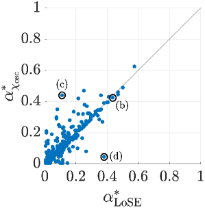
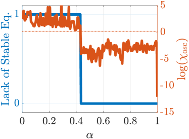
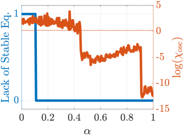
Figure 3: The consistency of LoSE (as a proxy for oscillations) and $\chi_{\rm osc}$ (as a “ground truth” measure of oscillations) when locally sweeping between network parameters that give rise to oscillations and those that do not. (a) The value of $\alpha$ at which LoSE switches vs. the value of $\alpha$ at which $\log(\chi_{\rm osc})$ crosses the threshold $\vartheta$. Note the gathering of the majority of the points around the $\alpha^{*}_{\chi_{\rm osc}}=\alpha^{*}_{\rm LoSE}$ line. (b-d) Sample plots of LoSE (left vertical axis) and $\log(\chi_{\rm osc})$ (right vertical axis) as a function of $\alpha$ for three sample cases denoted in panel (a). The red horizontal dotted line indicate the oscillation threshold $\vartheta$. Panel (b) illustrates a common mid-point scenario where $\alpha^{*}_{\chi_{\rm osc}}\simeq\alpha^{*}_{\rm LoSE}$ while (c) and (d) illustrate two extreme conditions.

A.3 Global Inspection in Networks of E-I Pairs

In Sections A.1 and A.2, we have inspected general excitatory-inhibitory networks with arbitrary connection patterns between the nodes. Here, we inspect the networks of E-I pairs studied in Section 4. These networks not only constitute an important special case from a computational neuroscience standpoint, but they also lend themselves to theoretical characterizations such as that in Theorem 4.1. Here, we inspect the quality of LoSE as a proxy for oscillations using the theoretical condition in (24). To this end, we construct random networks according to

$$d_{i}\sim\mathcal{U}(0,d_{\max}),\quad a_{i}\sim\mathcal{U}(a_{\min},a_{\max}),\ a_{\min}>d_{\max}+2,$$

$$b_{i}=c_{i}\sim\mathcal{U}(b_{\min},b_{\max}),\ b_{\min}>\sqrt{(a_{\max}-1)(d_{\max}+1)},$$

$$m_{j,i}\sim\mathcal{U}(m_{j,\min},m_{j,\max}),\ m_{2,\min}>\frac{a_{\max}-1}{b_{\min}}m_{1,\max},$$

$$\tau_{i}\sim\mathcal{U}(\tau_{\min},\tau_{\max}),\ \ {\rm i.i.d.}\ \forall j=1,2,i\in\{1,\dots,n\},$$ (28)

all satisfying (4a)-(4c). The values of $u_{i,1}$ and $u_{i,2}$ are chosen at the center of their respective ranges in (4d)-(4e) so that the E-I pairs oscillate at their maximum amplitude before interconnection. For $\mathbf{A}$, we first generate a random $\mathbf{G}\in\mathbb{R}_{\geq 0}^{n\times n}$ with zero diagonal and set $\mathbf{A}=\eta\bar{\mathbf{A}}$, $\bar{\mathbf{A}}={\rm diag}(\bar{\mathbf{u}}_{1}-\mathbf{u}_{1})\mathbf{G}[{\rm diag}(\mathbf{G}\mathbf{1}_{n}){\rm diag}(\mathbf{m}_{1})]^{-1}$. $\mathbf{A}$ then satisfies (24) for all $i\in\{1,\dots,n\}$ iff $\eta\in[0,1)$.

Figure 4 shows the distribution of $\log\chi_{\rm osc}$ for random networks of $n=10$ oscillators, $\epsilon=0.1$, and varying interconnection strength $\eta$. For disconnected oscillators $(\eta=0)$, each oscillator has a perfectly regular oscillation (by Theorem 3.1) and thus very large $\chi_{\rm osc}$ (though finite, due to the finiteness of $\chi_{\rm reg}$, which is in turn due to finite signal length and numerical error). These oscillations lose their regularity and/or strength as we increase the connection strength $\eta$ towards $1$, but still persist up to $\eta=0.99$, showing the almost sufficiency of (24). Moving beyond $\eta=1$, almost no oscillations persist even at $\eta=1.01$ (and less so at $\eta=1.1$) due to convergence to the stable equilibria ensured by Theorem 4.1. This shows that (24) is also almost necessary for existence of oscillations in the network dynamics (23).

Figure 4: Strength and regularity of oscillations as a function of inter-oscillator connection strength ($\eta$). The probability density function of $\log\chi_{\rm osc}$ is plotted for $n=10$ and varying $\eta$. Each distribution is based on $1000$ random networks (A.3) with $d_{\max}=1$, $a_{\min}=3.5$, $a_{\max}=5$, $b_{\min}=\sqrt{8}+0.5$, $b_{\max}=\sqrt{8}+2$, $m_{1,\min}=1$, $m_{1,\max}=2$, $m_{2,\min}=8/b_{\min}+0.5$, $m_{2,\max}=8/b_{\min}+2$, $\tau_{\min}\!=\!1$, $\tau_{\max}\!=\!10$.

References

- Angeli and Sontag [2003] David Angeli and Eduardo D Sontag. Monotone control systems. IEEE Transactions on Automatic Control, 48(10):1684–1698, 2003.
- Baird [1986] B. Baird. Nonlinear dynamics of pattern formation and pattern recognition in the rabbit olfactory bulb. Physica D: Nonlinear Phenomena, 22(1-3):150–175, 1986.
- Berger [1929] H. Berger. Über das elektrenkephalogramm des menschen. Archiv für Psychiatrie und Nervenkrankheiten, 87(1):527–570, Dec 1929.
- Borisyuk and Kirillov [1992] R. M. Borisyuk and A. B. Kirillov. Bifurcation analysis of a neural network model. Biological Cybernetics, 66(4):319–325, 1992.
- Breakspear et al. [2010] M. Breakspear, S. Heitmann, and A. Daffertshofer. Generative models of cortical oscillations: neurobiological implications of the Kuramoto model. Frontiers in Human Neuroscience, 4:190, 2010.
- Breakspear et al. [2006] Michael Breakspear, JA Roberts, John R Terry, Serafim Rodrigues, N Mahant, and PA Robinson. A unifying explanation of primary generalized seizures through nonlinear brain modeling and bifurcation analysis. Cerebral Cortex, 16(9):1296–1313, 2006.
- Brouwer [1911] L. E. J. Brouwer. Über abbildung von mannigfaltigkeiten. Mathematische Annalen, 71(1):97–115, 1911.
- Bullo et al. [2009] F. Bullo, J. Cortés, and S. Martinez. Distributed Control of Robotic Networks. Applied Mathematics Series. Princeton University Press, 2009. ISBN 978-0-691-14195-4.
- Buzsáki and Draguhn [2004] G. Buzsáki and A. Draguhn. Neuronal oscillations in cortical networks. Science, 304(5679):1926–1929, 2004.
- Buzsaki [2006] Gyorgy Buzsaki. Rhythms of the Brain. Oxford University Press, 2006.
- Campbell and Wang [1996] S. Campbell and D. Wang. Synchronization and desynchronization in a network of locally coupled Wilson-Cowan oscillators. IEEE Transactions on Neural Networks, 7(3):541–554, 1996.
- Celi et al. [2021] F. Celi, A. Allibhoy, F. Pasqualetti, and J. Cortés. Linear-threshold dynamics for the study of epileptic events. IEEE Control Systems Letters, 5(4):1405–1410, 2021.
- Cole and Voytek [2017] S. R. Cole and B. Voytek. Brain oscillations and the importance of waveform shape. Trends in cognitive sciences, 21(2):137–149, 2017.
- Cowan et al. [2016] J. D. Cowan, J. Neuman, and W. van Drongelen. Wilson-Cowan equations for neocortical dynamics. The Journal of Mathematical Neuroscience, 6(1):1, 2016.
- Dayan and Abbott [2001] P. Dayan and L. F. Abbott. Theoretical Neuroscience: Computational and Mathematical Modeling of Neural Systems. Computational Neuroscience. MIT Press, Cambridge, MA, 2001.
- Destexhe and Sejnowski [2009] A. Destexhe and T. J. Sejnowski. The Wilson-Cowan model, 36 years later. Biological Cybernetics, 101(1):1–2, 2009.
- Donoghue et al. [2020] Thomas Donoghue, Matar Haller, Erik J Peterson, Paroma Varma, Priyadarshini Sebastian, Richard Gao, Torben Noto, Antonio H Lara, Joni D Wallis, Robert T Knight, Avgusta Shestyuk, and Bradley Voytek. Parameterizing neural power spectra into periodic and aperiodic components. Nature Neuroscience, 23(12):1655–1665, 2020.
- Ermentrout and Kopell [1990] G. B. Ermentrout and N. Kopell. Oscillator death in systems of coupled neural oscillators. SIAM Journal on Applied Mathematics, 50(1):125–146, 1990.
- Ermentrout and Terman [2010] G Bard Ermentrout and David H Terman. Mathematical foundations of neuroscience, volume 35. Springer Science & Business Media, 2010.
- Fries [2015] P. Fries. Rhythms for cognition: Communication through coherence. Neuron, 88:220–235, 2015.
- Grasman [1977] W. Grasman. Periodic solutions of autonomous differential equations in higher-dimensional spaces. The Rocky Mountain Journal of Mathematics, 7(3):457–466, 1977.
- Harris and Ermentrout [2015] Jeremy Harris and Bard Ermentrout. Bifurcations in the Wilson-Cowan equations with nonsmooth firing rate. SIAM Journal on Applied Dynamical Systems, 14(1):43–72, 2015.
- Hirsch and Smith [2006] Morris W Hirsch and Hal Smith. Monotone dynamical systems. In Handbook of differential equations: ordinary differential equations, volume 2, pages 239–357. Elsevier, 2006.
- Hopfield [1982] J. J. Hopfield. Neural networks and physical systems with emergent collective computational abilities. Proceedings of the National Academy of Sciences, 79(8):2554–2558, 1982.
- Hoppensteadt and Izhikevich [2012] Frank C Hoppensteadt and Eugene M Izhikevich. Weakly connected neural networks, volume 126. Springer Science & Business Media, 2012.
- Hülsemann et al. [2019] M. J. Hülsemann, E. Naumann, and B. Rasch. Quantification of phase-amplitude coupling in neuronal oscillations: Comparison of phase-locking value, mean vector length, modulation index, and generalized linear modeling cross-frequency coupling. Frontiers in neuroscience, 13:573, 2019.
- Hurwitz [1895] A. Hurwitz. Ueber die bedingungen, unter welchen eine gleichung nur wurzeln mit negativen reellen theilen besitzt. Mathematische Annalen, 46(1):273–284, 1895.
- Inagaki et al. [2019] H. K. Inagaki, L. Fontolan, S. Romani, and K. Svoboda. Discrete attractor dynamics underlies persistent activity in the frontal cortex. Nature, 566(7743):212–217, 2019.
- Izhikevich [2007] E. M. Izhikevich. Dynamical Systems in Neuroscience. MIT press, 2007.
- Jadi and Sejnowski [2014] M. P. Jadi and T. J. Sejnowski. Regulating cortical oscillations in an inhibition-stabilized network. Proceedings of the IEEE, 102(5):830–842, 2014.
- Johansson [2003] M. K. J. Johansson. Piecewise Linear Control Systems: A Computational Approach. Lecture Notes in Control and Information Sciences. Springer Berlin Heidelberg, 2003.
- Jones [2016] S. R. Jones. When brain rhythms aren’t ‘rhythmic’: implication for their mechanisms and meaning. Current Opinion in Neurobiology, 40:72–80, 2016.
- Kalitzin et al. [2019] S. Kalitzin, G. Petkov, P. Suffczynski, V. Grigorovsky, B. L. Bardakjian, F. Lopes da Silva, and P. L. Carlen. Epilepsy as a manifestation of a multistate network of oscillatory systems. Neurobiology of Disease, 130:104488, 2019.
- Kissinger et al. [2018] S. T. Kissinger, A. Pak, Y. Tang, S. C. Masmanidis, and A. A. Chubykin. Oscillatory encoding of visual stimulus familiarity. Journal of Neuroscience, 38(27):6223–6240, 2018.
- Liberzon [2003] D. Liberzon. Switching in Systems and Control. Systems & Control: Foundations & Applications. Birkhäuser, 2003.
- Mattia et al. [2013] M. Mattia, P. Pani, G. Mirabella, S. Costa, P. Del Giudice, and S. Ferraina. Heterogeneous attractor cell assemblies for motor planning in premotor cortex. Journal of Neuroscience, 33(27):11155–11168, 2013.
- Menara et al. [2020] T. Menara, G. Baggio, D. S. Bassett, and F. Pasqualetti. Stability conditions for cluster synchronization in networks of heterogeneous Kuramoto oscillators. IEEE Transactions on Control of Network Systems, 7(1):302–314, 2020.
- Monteiro et al. [2002] L. H. A. Monteiro, M. A. Bussab, and J. G. C. Berlinck. Analytical results on a Wilson-Cowan neuronal network modified model. Journal of Theoretical Biology, 219(1):83–91, 2002.
- Morrison et al. [2016] K. Morrison, A. Degeratu, V. Itskov, and C. Curto. Diversity of emergent dynamics in competitive threshold-linear networks: a preliminary report. arXiv preprint arXiv:1605.04463, 2016.
- Muldoon et al. [2016] S. F. Muldoon, F. Pasqualetti, S. Gu, M. Cieslak, S. T. Grafton, J. M. Vettel, and D. S. Bassett. Stimulation-based control of dynamic brain networks. PLOS Computational Biology, 12(9):e1005076, 2016.
- Nozari and Cortés [2019] E. Nozari and J. Cortés. Oscillations and coupling in interconnections of two-dimensional brain networks. In American Control Conference, pages 193–198, Philadelphia, PA, July 2019.
- Nozari and Cortés [2021] E. Nozari and J. Cortés. Hierarchical selective recruitment in linear-threshold brain networks. Part I: Intra-layer dynamics and selective inhibition. IEEE Transactions on Automatic Control, 66(3):949–964, 2021.
- Onslow et al. [2014] A. C. E. Onslow, M. W. Jones, and R. Bogacz. A canonical circuit for generating phase-amplitude coupling. PLOS One, 9(8):e102591, 2014.
- Papadopoulos et al. [2020] L. Papadopoulos, C. W. Lynn, D. Battaglia, and D. S. Bassett. Relations between large-scale brain connectivity and effects of regional stimulation depend on collective dynamical state. PLOS Computational Biology, 16(9):1–43, 09 2020.
- Perko [2000] L. Perko. Differential Equations and Dynamical Systems, volume 7 of Texts in Applied Mathematics. Springer, New York, 3rd edition, 2000.
- Quentin et al. [2019] R. Quentin, J. King, E. Sallard, N. Fishman, R. Thompson, E. R. Buch, and L. G. Cohen. Differential brain mechanisms of selection and maintenance of information during working memory. Journal of Neuroscience, 39(19):3728–3740, 2019.
- Răsvan [2007] Vl Răsvan. A new dissipativity criterion—towards yakubovich oscillations. International Journal of Robust and Nonlinear Control: IFAC-Affiliated Journal, 17(5-6):483–495, 2007.
- Sanchez [2010] L. A. Sanchez. Existence of periodic orbits for high-dimensional autonomous systems. Journal of Mathematical Analysis and Applications, 363(2):409–418, 2010.
- Sase et al. [2017] Takumi Sase, Yuichi Katori, Motomasa Komuro, and Kazuyuki Aihara. Bifurcation analysis on phase-amplitude cross-frequency coupling in neural networks with dynamic synapses. Frontiers in computational neuroscience, 11:18, 2017.
- Schuster and Wagner [1990] H. G. Schuster and P. Wagner. A model for neuronal oscillations in the visual cortex. 1. mean-field theory and derivation of the phase equations. Biological Cybernetics, 64(1):77–82, 1990.
- Segneri et al. [2020] Marco Segneri, Hongjie Bi, Simona Olmi, and Alessandro Torcini. Theta-nested gamma oscillations in next generation neural mass models. Frontiers in computational neuroscience, 14:47, 2020.
- Simic et al. [2002] S. Simic, K. H. Johansson, J. Lygeros, and S. Sastry. Hybrid limit cycles and hybrid Poincaré-Bendixson. In IFAC World Congress, 2002.
- Steriade [2006] M. Steriade. Grouping of brain rhythms in corticothalamic systems. Neuroscience, 137(4):1087–1106, 2006.
- Tang et al. [2007] A. Kevin Tang, A. Simsek, A. Ozdaglar, and D. Acemoglu. On the stability of p-matrices. Linear Algebra and its Applications, 426(1):22–32, 2007.
- Tomberg and Yakubovich [1989] EA Tomberg and Vladimir Andreevich Yakubovich. Conditions for auto-oscillations in nonlinear systems. Siberian Mathematical Journal, 30(4):641–653, 1989.
- Tort-Colet et al. [2019] N. Tort-Colet, C. Capone, M. V. Sanchez-Vives, and M. Mattia. Attractor competition enriches cortical dynamics during awakening from anesthesia. bioRxiv, 2019. URL https://www.biorxiv.org/content/early/2019/01/10/517102.
- van Ede et al. [2018] F. van Ede, A. J. Quinn, M. W. Woolrich, and A. C. Nobre. Neural oscillations: sustained rhythms or transient burst-events? Trends in Neurosciences, 41(7):415–417, 2018.
- Wang [2010] X. Wang. Neurophysiological and computational principles of cortical rhythms in cognition. Physiological Reviews, 90(3):1195–1268, 2010.
- White et al. [1995] John A White, Thomas Budde, and Alan R Kay. A bifurcation analysis of neuronal subthreshold oscillations. Biophysical Journal, 69(4):1203–1217, 1995.
- Whittington et al. [2000] M. A. Whittington, R. D. Traub, N. Kopell, B. Ermentrout, and E. H. Buhl. Inhibition-based rhythms: experimental and mathematical observations on network dynamics. International Journal of Psychophysiology, 38(3):315–336, 2000.
- Wilson and Cowan [1972] H. R. Wilson and J. D. Cowan. Excitatory and inhibitory interactions in localized populations of model neurons. Biophysical Journal, 12(1):1–24, 1972.