Grad-Match: Gradient Matching based Data Subset Selection for Efficient Deep Model Training

Abstract

The great success of modern machine learning models on large datasets is contingent on extensive computational resources with high financial and environmental costs. One way to address this is by extracting subsets that generalize on par with the full data. In this work, we propose a general framework, Grad-Match, which finds subsets that closely match the gradient of the training or validation set. We find such subsets effectively using an orthogonal matching pursuit algorithm. We show rigorous theoretical and convergence guarantees of the proposed algorithm and, through our extensive experiments on real-world datasets, show the effectiveness of our proposed framework. We show that Grad-Match significantly and consistently outperforms several recent data-selection algorithms and achieves the best accuracy-efficiency trade-off. Grad-Match is available as a part of the CORDS toolkit: https://github.com/decile-team/cords.

1 Introduction

Modern machine learning systems, especially deep learning frameworks, have become very computationally expensive and data-hungry. Massive training datasets have significantly increased end-to-end training times, computational and resource costs (Sharir et al., 2020), energy requirements (Strubell et al., 2019), and carbon footprint (Schwartz et al., 2019). Moreover, most machine learning models require extensive hyper-parameter tuning, further increasing the cost and time, especially on massive datasets. In this paper, we study efficient machine learning through the paradigm of subset selection, which seeks to answer the following question: Can we train a machine learning model on much smaller subsets of a large dataset, with negligible loss in test accuracy?

Data subset selection enables efficient learning at multiple levels. First, by using a subset of a large dataset, we can enable learning on relatively low resource computational environments without requiring a large number of GPU and CPU servers. Second, since we are training on a subset of the training dataset, we can significantly improve the end-to-end turnaround time, which often requires multiple training runs for hyper-parameter tuning. Finally, this also enables significant reduction in the energy consumption and CO2 emissions of deep learning (Strubell et al., 2019), particularly since a large number of deep learning experiments need to be run in practice. Recently, there have been several efforts to make machine learning models more efficient via data subset selection (Wei et al., 2014a; Kaushal et al., 2019; Coleman et al., 2020; Har-Peled & Mazumdar, 2004; Clarkson, 2010; Mirzasoleiman et al., 2020a; Killamsetty et al., 2021). Existing approaches either use proxy functions to select data points, or are specific to particular machine learning models, or use approximations of quantities such as gradient error or generalization errors. In this work, we propose a data selection framework called Grad-Match, which exactly minimizes a residual error term obtained by analyzing adaptive data subset selection algorithms, therefore admitting theoretical guarantees on convergence.

1.1 Contributions of this work

Analyses of convergence bounds of adaptive data subset selection algorithms. A growing number of recent approaches (Mirzasoleiman et al., 2020a; Killamsetty et al., 2021) can be cast within the framework of adaptive data subset selection, where the data subset selection algorithm (which selects the data subset depending on specific criteria) is applied in conjunction with the model training. As the model training proceeds, the subset on which the model is being trained is improved via the current model’s snapshots. We analyze the convergence of this general framework and show that the convergence bound critically depends on an additive error term depending on how well the subset’s weighted gradients match either the full training gradients or the full validation gradients (c.f., Section 2).

Data selection framework with convergence guarantees. Inspired by the result above, we present Grad-Match, a gradient-matching algorithm (c.f., Section 3), which directly tries to minimize the gradient matching error. As a result, we are able to show convergence bounds for a large class of convex loss functions. We also argue that the resulting bounds we obtain are tighter than those of recent works (Mirzasoleiman et al., 2020a; Killamsetty et al., 2021), which either use upper bounds or their approximations. We then show that minimizing the gradient error can be cast as a weakly submodular maximization problem and propose an orthogonal matching pursuit based greedy algorithm. We then propose several implementation tricks (c.f., Section 4), which provide significant speedups for the data selection step.

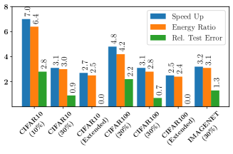
Figure 1: Efficiency of Grad-Match relative to full training on the CIFAR-10, CIFAR-100, and Imagenet datasets.

Best tradeoff between efficiency and accuracy. In our empirical results (c.f., Section 5), we show that Grad-Match achieves much a better accuracy and training-time trade-off than several state-of-the-art approaches such as Craig (Mirzasoleiman et al., 2020a), Glister (Killamsetty et al., 2021), random subsets, and even full training with early stopping. When training with ResNet-18 on Imagenet, CIFAR-10, and CIFAR-100, we observe around 3$\times$ efficiency improvement with an accuracy drop of close to 1% for 30% subset. With smaller subsets (e.g., 20% and 10%), we sacrifice a little more in terms of accuracy (e.g., 2% and 2.8%) for a larger speedup in training (4$\times$ and 7$\times$). Furthermore, we see that by extending the training beyond the specified number of epochs (300 in this case), we can match the accuracy on the full dataset using just 30% of the data while being overall 2.5$\times$ faster. In the case of MNIST, the speedup improvements are even more drastic, ranging from 27$\times$ to 12$\times$ with 0.35% to 0.05% accuracy degradation.

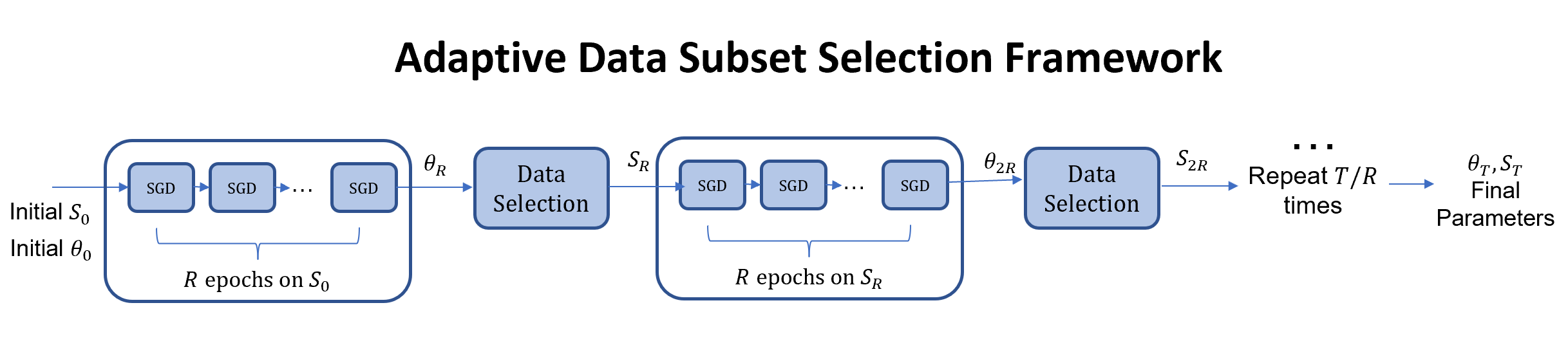
Figure 2: Block Diagram of any adaptive data selection algorithm, where data selection is performed every $R$ epochs of (stochastic) gradient descent, and the gradient descent updates are performed on the subsets obtained by the data selection.

1.2 Related work

A number of recent papers have used submodular functions as proxy functions (Wei et al., 2014a, c; Kirchhoff & Bilmes, 2014; Kaushal et al., 2019) (to actual loss). Let $n$ be the number of data points in the ground set. Then a set function $f:2^{[n]}\rightarrow\mathbf{R}$ is submodular  (Fujishige, 2005) if it satisfies the diminishing returns property: for subsets $S,T\subseteq[n],f(j|S)\triangleq f(S\cup j)-f(S)\geq f(j|T)$. Another commonly used approach is that of coresets. Coresets are weighted subsets of the data, which approximate certain desirable characteristics of the full data (, e.g., the loss function) (Feldman, 2020). Coreset algorithms have been used for several problems including $k$-means and $k$-median clustering (Har-Peled & Mazumdar, 2004), SVMs (Clarkson, 2010) and Bayesian inference (Campbell & Broderick, 2018). Coreset algorithms require algorithms that are often specialized and very specific to the model and problem at hand and have had limited success in deep learning.

A very recent coreset algorithm called Craig (Mirzasoleiman et al., 2020a) has shown promise for both deep learning and classical machine learning models such as logistic regression. Unlike other coreset techniques that largely focus on approximating loss functions, Craig selects representative subsets of the training data that closely approximate the full gradient. Another approach poses the data selection as a discrete bi-level optimization problem and shows that, for several choices of loss functions and models (Killamsetty et al., 2021; Wei et al., 2015), the resulting optimization problem is submodular. A few recent papers have studied data selection approaches for robust learning. Mirzasoleiman et al. (2020b) extend Craig to handle noise in the data, whereas Killamsetty et al. (2021) study class imbalance and noisy data settings by assuming access to a clean validation set. In this paper, we study data selection under class imbalance in a setting similar to (Killamsetty et al., 2021), where we assume access to a clean validation set. Our work is also related to highly distributed deep learning systems (Jia et al., 2018) which make deep learning significantly faster using a cluster of hundreds of GPUs. In this work, we instead focus on single GPU training runs, which are more practical for smaller companies and academic labs and potentially complementary to (Jia et al., 2018). Finally, our work is also complementary to that of (Wang et al., 2019), where the authors employ tricks such as selective layer updates, low-precision backpropagation, and random subsampling to achieve significant energy reductions. In this work, we demonstrate both energy and time savings solely based on a more principled subset selection approach.

2 Grad-Match through the lens of adaptive data subset selection

In this section, we will study the convergence of general adaptive subset selection algorithms and use the result (Theorem 1) to motivate Grad-Match.

Notation. Denote $\mathcal{U}=\{(x_{i},y_{i})\}_{i=1}^{N}$, as the set of training examples, and let $\mathcal{V}=\{(x_{j},y_{j})\}_{j=1}^{M}$ denote the validation set. Let $\theta$ be the classifier model parameters. Next, denote by $L_{T}^{i}(\theta)=L_{T}(x_{i},y_{i},\theta)$, the training loss at the $i^{th}$ epoch of training, and let $L_{T}(\mathcal{X},\theta)=\sum_{i\in\mathcal{X}}L_{T}(x_{i},y_{i},\theta)$ be the loss on a subset $\mathcal{X}\subseteq\mathcal{U}$ of the training examples. Let the validation loss be denoted by $L_{V}$. In Table 1 in Appendix A, we organize and tabulate the notations used throughout this paper.

Adaptive data subset selection: (Stochastic) gradient descent algorithms proceed by computing the gradients of all the training data points for $T$ epochs. We study the alternative approach of adaptive data selection, in which training is performed using a weighted sum of gradients of the training data subset instead of the full training data. In the adaptive data selection approach, the data selection is performed in conjunction with training such that subsets get incrementally refined as the learning algorithm proceeds. This incremental subset refinement allows the data selection to adapt to the learning and produces increasingly effective subsets with progress of the learning algorithm. Assume that an adaptive data selection algorithm produces weights $\mathbf{w}^{t}$ and subsets $\mathcal{X}^{t}$ for $t=1,2,\cdots,T$ through the course of the algorithm. In other words, at iteration $t$, the parameters $\theta_{t}$ are updated using the weighted loss of the model on subset $\mathcal{X}^{t}$ by weighing each example $i\in\mathcal{X}^{t}$ with its corresponding weight $w^{t}_{i}$. For example, if we use gradient descent, we can write the update step as: $\theta_{t+1}=\theta_{t}-\alpha\sum_{i\in\mathcal{X}^{t}}w^{t}_{i}\nabla_{\theta}L_{T}(x_{i},y_{i},\theta_{t})$. Note that though this framework uses a potentially different set $\mathcal{X}^{t}$ in each iteration $t$, we need not perform data selection every epoch. In fact, in practice, we run data selection only every $R$ epochs, in which case, the same subsets and weights will be used between epochs $t=R\tau$ and $t=R(\tau+1)$. In contrast, the non-adaptive data selection settings (Wei et al., 2014b, c; Kaushal et al., 2019) employ the same $\mathcal{X}^{t}=\mathcal{X}$ for gradient descent in every iteration. In Figure 2, we present the broad adaptive data selection scheme. In this work, we focus on a setting in which the subset size is fixed, i.e., $|\mathcal{X}^{t}|=k$ (typically a small fraction of the training dataset).

Convergence analysis: We now study the conditions for the convergence of either the full training loss or the validation loss achieved by any adaptive data selection strategy. Recall that we can characterize any data selection algorithm by a set of weights $\mathbf{w}^{t}$ and subsets $\mathcal{X}^{t}$ for $t=1,\cdots,T$. We provide a convergence result which holds for any adaptive data selection algorithm, and applies to Lipschitz continuous, Lipschitz smooth, and strongly convex loss functions. Before presenting the result, we define the term:

$$\small\mbox{Err}(\mathbf{w}^{t},\mathcal{X}^{t},L,L_{T},\theta_{t})={\left\|\sum_{i\in\mathcal{X}^{t}}w^{t}_{i}\nabla_{\theta}L_{T}^{i}(\theta_{t})-\nabla_{\theta}L(\theta_{t})\right\|}$$

The norm considered in the above equation is the l2 norm. Next, assume that the parameters satisfy $||\theta||^{2}\leq D^{2}$, and let $L$ denote either the training or validation loss. We next state the convergence result:

Theorem 1.

Any adaptive data selection algorithm. run with full gradient descent (GD), defined via weights $\mathbf{w}^{t}$ and subsets $\mathcal{X}^{t}$ for $t=1,\cdots,T$, enjoys the following guarantees:
(1). If $L_{T}$ is Lipschitz continuous with parameter $\sigma_{T}$, optimal model parameters are $\theta^{*}$, and $\alpha=\frac{D}{\sigma_{T}\sqrt{T}}$, then $\min_{t=1:T}L(\theta_{t})-L(\theta^{*})\leq\frac{D\sigma_{T}}{\sqrt{T}}+\frac{D}{T}\sum_{t=1}^{T-1}\mbox{Err}(\mathbf{w}^{t},\mathcal{X}^{t},L,L_{T},\theta_{t})$.
(2) If $L_{T}$ is Lipschitz smooth with parameter $\mathcal{L}_{T}$, optimal model parameters are $\theta^{*}$, and $L_{T}^{i}$ satisfies $0\leq L_{T}^{i}(\theta)\leq\beta_{T}$, $\forall i$, then setting $\alpha=1/{\mathcal{L}_{T}}$, we have $\min_{t=1:T}L(\theta_{t})-L(\theta^{*})\leq\frac{D^{2}\mathcal{L}_{T}+2\beta_{T}}{2T}+\frac{D}{T}\sum_{t=1}^{T-1}\mbox{Err}(\mathbf{w}^{t},\mathcal{X}^{t},L,L_{T},\theta_{t})$.
(3) If $L_{T}$ is Lipschitz continuous with parameter $\sigma_{T}$, optimal model parameters are $\theta^{*}$, and $L$ is strongly convex with parameter $\mu$, then setting a learning rate $\alpha_{t}=\frac{2}{\mu(1+t)}$, we have $\min_{t=1:T}L(\theta_{t})-L(\theta^{*})\leq\frac{2{\sigma_{T}}^{2}}{\mu(T+1)}+\sum_{t=1}^{t=T}\frac{2Dt}{T(T+1)}\mbox{Err}(\mathbf{w}^{t},\mathcal{X}^{t},L,L_{T},\theta_{t})$.

We present the proof in Appendix B.1. We can also extend this result to the case in which SGD is used instead of full GD to update the model. The main difference in the result is that the inequality holds with expectations over both sides. We defer the convergence result and proof to Appendix B.2. Theorem 1 suggests that an effective data selection algorithm should try to obtain subsets which have very small error $\mbox{Err}(\mathbf{w}^{t},\mathcal{X}^{t},L,L_{T},\theta_{t})$ for $t=1,\cdots,T$. If the goal of data selection is to select a subset $\mathcal{X}^{t}$ at every epoch which approximates the full training set, the data selection procedure should try to minimize $\mbox{Err}(\mathbf{w}^{t},\mathcal{X}^{t},L_{T},L_{T},\theta_{t})$. On the other hand, to select subset $\mathcal{X}^{t}$ at every epoch which approximates the validation set, the data selection procedure should try to minimize $\mbox{Err}(\mathbf{w}^{t},\mathcal{X}^{t},L_{V},L_{T},\theta_{t})$. In Appendix B.3, we provide conditions under which an adaptive data selection approach reduces the loss function $L$ (which can either be the training loss $L_{T}$ or the validation loss $L_{V}$). In particular, we show that any data selection approach which attempts to minimize the error term $\mbox{Err}(\mathbf{w}^{t},\mathcal{X}^{t},L,L_{T},\theta_{t})$ is also likely to reduce the loss value at every iteration. In the next section, we present Grad-Match, that directly minimizes this error function $\mbox{Err}(\mathbf{w}^{t},\mathcal{X}^{t},L,L_{T},\theta_{t})$.

3 The Grad-Match Algorithm

Following the result of Theorem 1, we now design an adaptive data selection algorithm that minimizes the gradient error term: $\mbox{Err}(\mathbf{w}^{t},\mathcal{X}^{t},L,L_{T},\theta_{t})$ (where $L$ is either the training loss or the validation loss) as the training proceeds. The complete algorithm is shown in Algorithm 1. In Algorithm 1, isValid is a boolean Validation flag indicator that indicates whether to match the subset loss gradient with validation set loss gradient like in the case of class imbalance (isValid=True) or training set loss gradient (isValid=False). As discussed in Section 2, we do the subset selection only every $R$ epochs, and during the rest of the epochs, we update the model parameters (using Batch SGD) on the previously chosen set $\mathcal{X}^{t}$ with associated weights $\mathbf{w}^{t}$. This ensures that the subset selection time in itself is negligible compared to the training time, thereby ensuring that the adaptive selection runs as fast as simple random selection. The full algorithm is shown in Algorithm 1. Line 9 of Algorithm 1 is the mini-batch SGD and takes as inputs the weights, subset of instances, learning rate, training loss, batch size, and the number of epochs. We randomly shuffle elements in the subset $\mathcal{X}^{t}$, divide them up into mini-batches of size $B$, and run mini-batch SGD with instance weights.

Lines 3 and 5 in Algorithm 1 are the data subset selection steps, run either with the full training gradients or validation gradients. We basically minimize the error term $\mbox{Err}(\mathbf{w}^{t},\mathcal{X}^{t},L,L_{T},\theta_{t})$ with minor difference. Define the regularized version of $\mbox{Err}(\mathbf{w}^{t},\mathcal{X}^{t},L,L_{T},\theta_{t})$ as:

$$\mbox{Err}_{\lambda}(\mathbf{w},\mathcal{X},L,L_{T},\theta_{t})= \mbox{Err}(\mathbf{w},\mathcal{X},L,L_{T},\theta_{t})+\lambda\|\mathbf{w}\|^{2}$$ (1)

The data selection optimization problem then is:

$$\mathbf{w}^{t},\mathcal{X}^{t}=\underset{\mathbf{w},\mathcal{X}:|\mathcal{X}|\leq k}{\mathop{\mathrm{argmin}}}\mbox{Err}_{\lambda}(\mathbf{w},\mathcal{X},L,L_{T},\theta_{t})$$ (2)

In $\mbox{Err}_{\lambda}(\mathbf{w},\mathcal{X},L,L_{T},\theta_{t})$, the first term is the additional error term that adaptive subset algorithms have from the convergence analysis discussed in Section 2, and the second term is a squared l2 loss regularizer over the weight vector $\mathbf{w}$ with a regularization coefficient $\lambda$ to prevent overfitting by discouraging the assignment of large weights to individual data instances or mini-batches. During data-selection, we select the weights $\mathbf{w}^{t}$ and subset $\mathcal{X}^{t}$ by optimizing equation (2). To this end, we define:

$$E_{\lambda}(\mathcal{X})=\min_{\mathbf{w}}\mbox{Err}_{\lambda}(\mathbf{w},\mathcal{X},L,L_{T},\theta_{t})$$ (3)

Note that the optimization problem in Eq. (2) is equivalent to solving the optimization problem $\min_{\mathcal{X}:|\mathcal{X}|\leq k}E_{\lambda}(\mathcal{X})$. The detailed optimization algorithm is presented in Section 3.1.

Grad-Match for mini-batch SGD: We now discuss an alternative formulation of Grad-Match, specifically for mini-batch SGD. Recall from Theorem 1 and optimization problem (2), that in the case of full gradient descent or SGD, we select a subset of data points for the data selection. However, mini-batch SGD is a combination of SGD and full gradient descent, where we randomly select a mini-batch and compute the full gradient on that mini-batch. To handle this, we consider a variant of Grad-Match, which we refer to as Grad-MatchPB. Here we select a subset of mini-batches by matching the weighted sum of mini-batch training gradients to the full training loss (or validation loss) gradients. Once we select a subset of mini-batches, we train the neural network on the mini-batches, weighing each mini-batch by its corresponding weight. Let $B$ be the batch size, $b_{n}=n/B$ as the total number of mini-batches, and $b_{k}=k/B$ as the number of batches to be selected. Let $\nabla_{\theta}L_{T}^{B_{1}}(\theta_{t}),\cdots,\nabla_{\theta}L_{T}^{B_{b_{n}}}(\theta_{t})$ denote the mini-batch gradients. The optimization problem is then to minimize $E^{B}_{\lambda}(\mathcal{X})$, which is defined as:

$$E^{B}_{\lambda}(\mathcal{X})=\min_{\mathbf{w}}\lVert\sum_{i\in\mathcal{X}}w^{i}_{t}\nabla_{\theta}L_{T}^{B_{i}}(\theta_{t})-\nabla_{\theta}L(\theta_{t})\rVert+\lambda\lVert\mathbf{w}\rVert^{2}$$

The constraint now is $|\mathcal{X}|\leq b_{k}$, where $\mathcal{X}$ is a subset of mini-batches instead of being a subset of data points. The use of mini-batches considerably reduces the number of selection rounds during the OMP algorithm by a factor of $B$, resulting in $B\times$ speed up. In our experiments, we compare the performance of Grad-Match and Grad-MatchPB  and show that Grad-MatchPB is considerably more efficient while being comparable in performance. Grad-MatchPB is a simple modification to lines 3 and 5 of Algorithm 1, where we send the mini-batch gradients instead of individual gradients to the orthogonal matching pursuit (OMP) algorithm (discussed in the next section). Further, we use the subset of mini-batches selected directly without any additional shuffling or sampling in our current experiments. We will consider augmenting the selected mini-batch subsets with additional shuffling or including new mini-batches with augmented images in our future work.

Algorithm 1 Grad-Match Algorithm

0:  Train set: ${\mathcal{U}}$; validation set: ${\mathcal{V}}$; initial subset: $\mathcal{X}^{(0)}$; subset size: $k$; TOL: $\epsilon$; initial params: $\theta_{0}$; learning rate: $\alpha$; total epochs: $T$, selection interval: $R$, Validation Flag: isValid, Batchsize: $B$

1:  for epochs $t$ in $1,\cdots,T$ do

2:    if $(t\mbox{ mod }R==0)$ and $(\mbox{isValid}==1)$ then

3:       $\mathcal{X}^{t},\mathbf{w}^{t}=\operatorname{OMP}(L_{T},L_{V},\theta_{t},k,\epsilon)$

4:    else if $(t\mbox{ mod }R==0)$ and $(\mbox{isValid}==0)$ then

5:       $\mathcal{X}^{t},\mathbf{w}^{t}=\operatorname{OMP}(L_{T},L_{T},\theta_{t},k,\epsilon)$

6:    else

7:       $\mathcal{X}^{t}=\mathcal{X}^{t-1}$

8:    end if

9:    $\theta_{t+1}=\mbox{BatchSGD}(\mathcal{X}^{t},\mathbf{w}^{t},\alpha,L_{T},B,\mbox{Epochs}=1)$

10:  end for

11:  Output final model parameters $\theta_{T}$

3.1 Orthogonal Matching Pursuit (OMP) algorithm

We next study the optimization algorithm for solving equation (2). Our objective is to minimize $E_{\lambda}(\mathcal{X})$ subject to the constraint $\mathcal{X}:|\mathcal{X}|\leq k$. We can also convert this into a maximization problem. For that, define: $F_{\lambda}(\mathcal{X})=L_{\max}-\min_{\mathbf{w}}\mbox{Err}_{\lambda}(\mathcal{X},\mathbf{w},L,L_{T},\theta_{t})$. Note that we minimize $E_{\lambda}(\mathcal{X})$ subject to the constraint $\mathcal{X}:|\mathcal{X}|\leq k$ until $E_{\lambda}(\mathcal{X})\leq\epsilon$, where $\epsilon$ is the tolerance level.

Algorithm 2 OMP

0:  Training loss $L_{T}$, target loss: $L$, current parameters: $\theta$, regularization coefficient: $\lambda$, subset size: $k$, tolerance: $\epsilon$

  $\mathcal{X}\leftarrow\emptyset$

  ${r}\leftarrow\nabla_{w}\mbox{Err}_{\lambda}(\mathcal{X},\mathbf{w},L,L_{T},\theta)|_{{\mathbf{w}}={0}}$

  while $|\mathcal{X}|\leq k$ and $E_{\lambda}(\mathcal{X})\geq\epsilon$ do

    $e=\text{argmax}_{j}|r_{j}|$

    $\mathcal{X}\leftarrow\mathcal{X}\cup\{e\}$

    ${\mathbf{w}}\leftarrow\text{argmin}_{{\mathbf{w}}}\mbox{Err}_{\lambda}(\mathcal{X},\mathbf{w},L,L_{T},\theta)$

    ${r}\leftarrow\nabla_{\mathbf{w}}\mbox{Err}_{\lambda}(\mathcal{X},\mathbf{w},L,L_{T},\theta)$

  end while

  return $\mathcal{X},\ {\mathbf{w}}$

Note that minimizing $E_{\lambda}$ is equivalent to maximizing $F_{\lambda}$. The following result shows that $F_{\lambda}$ is weakly submodular.

Theorem 2.

If $|\mathcal{X}|\leq k$ and $\max_{i}||\nabla_{\theta}L^{i}_{T}(\theta_{t})||_{2}<\nabla_{\max}$, then $F_{\lambda}(\mathcal{X})$ is $\gamma$-weakly submodular, with $\gamma\geq\frac{\lambda}{\lambda+k\nabla_{\max}^{2}}$

We present the proof in Appendix B.4. Recall that a set function $F:2^{[n]}\rightarrow\mathbb{R}$ is $\gamma$-weakly submodular (Gatmiry & Gomez-Rodriguez, 2018; Das & Kempe, 2011) if $F(j|S)\geq\gamma F(j|T),S\subseteq T\subseteq[n]$. Since $F_{\lambda}(\mathcal{X})$ is approximately submodular (Das & Kempe, 2011), a greedy algorithm (Nemhauser et al., 1978; Das & Kempe, 2011; Elenberg et al., 2018) admits a $(1-\exp(-\gamma))$ approximation guarantee. While the greedy algorithm is very appealing, it needs to compute the gain $F_{\lambda}(j|\mathcal{X})$, $O(nk)$ number of times. Since computation of each gain involves solving a least squares problem, this step will be computationally expensive, thereby defeating the purpose of data selection. To address this issue, we consider a slightly different algorithm, called the orthogonal matching pursuit (OMP) algorithm, studied in (Elenberg et al., 2018). We present OMP in Algorithm 2. In the corollary below, we provide the approximation guarantee for Algorithm 2.

Corollary 1.

Algorithm 2, when run with a cardinality constraint $|\mathcal{X}|\leq k$ returns a $1-\exp\left(\frac{-\lambda}{\lambda+k\nabla_{\max}^{2}}\right)$ approximation for maximizing $F_{\lambda}(\mathcal{X})$ with $\mathcal{X}:|\mathcal{X}|\leq k$.

We can also find the minimum sized subset such that the resulting error $E_{\lambda}(\mathcal{X})\leq\epsilon$. We note that this problem is essentially: $\min_{\mathcal{X}}|\mathcal{X}|$ such that $F_{\lambda}(\mathcal{X})\geq L_{\max}-\epsilon$. This is a weakly submodular set cover problem, and the following theorem shows that a greedy algorithm (Wolsey, 1982) as well as OMP (Algorithm 2) with a stopping criterion $E_{\lambda}(\mathcal{X})\leq\epsilon$ achieve the following approximation bound:

Theorem 3.

If the function $F_{\lambda}(\mathcal{X})$ is $\gamma$-weakly submodular, $\mathcal{X}^{*}$ is the optimal subset and $\max_{i}||\nabla_{\theta}L^{i}_{T}(\theta_{t})||_{2}<\nabla_{\max}$, (both) the greedy algorithm and OMP (Algorithm 2), run with stopping criteria $E_{\lambda}(\mathcal{X})\leq\epsilon$ result in sets $\mathcal{X}$ such that $|\mathcal{X}|\leq\frac{|\mathcal{X}^{*}|}{\gamma}\log\left(\frac{L_{\max}}{\epsilon}\right)$ where $L_{\max}$ is an upper bound of $F_{\lambda}$ .

The proof of this theorem is in Appendix B.5. Finally, we derive the convergence result for Grad-Match as a corollary of Theorem 1. In particular, assume that by running OMP, we can achieve sets $\mathcal{X}^{t}$ such that $E_{\lambda}(\mathcal{X}^{t})\leq\epsilon$, for all $t=1,\cdots,T$. If $L$ is Lipschitz continuous, we obtain a convergence bound of $\min_{t}L(\theta_{t})-L(\theta^{*})\leq\frac{D\sigma_{T}}{\sqrt{T}}+D\epsilon$. In the case of smooth or strongly convex functions, the result can be improved to $O(1/T)$. For example, with smooth functions, we have: $\min_{t}L(\theta_{t})-L(\theta^{*})\leq\frac{D^{2}\mathcal{L}_{T}+2\beta_{T}}{2T}+D\epsilon$. More details can be found in Appendix B.6.

3.2 Connections to existing work

Next, we discuss connections of Grad-Match to existing approaches such as Craig and Glister, and contrast the resulting theoretical bounds. Let $\mathcal{X}$ be a subset of $k$ data points from the training or validation set. Consider the expression for loss $L(\theta)=\sum_{i\in\mathcal{W}}L(x_{i},y_{i},\theta)$ so that $L=L_{T}$ when $\mathcal{W}=\mathcal{U}$ and $L=L_{V}$ when $\mathcal{W}=\mathcal{V}$. Define $\hat{E}(\mathcal{X})$ to be:

$$\hat{E}(\mathcal{X}) =\sum_{i\in\mathcal{W}}\min_{j\in\mathcal{X}}\|\nabla_{\theta}L^{i}(\theta_{t})-\nabla_{\theta}L_{T}^{j}(\theta_{t})\|$$ (4)

Note that $\hat{E}(\mathcal{X})$ is an upper bound for $E(\mathcal{X})$ (Mirzasoleiman et al., 2020a):

$$E(\mathcal{X}) =\min_{\mathbf{w}}\mbox{Err}({\mathbf{w}},\mathcal{X},L,L_{T},\theta_{t})\leq\hat{E}(\mathcal{X})$$ (5)

Given the set $\mathcal{X}^{t}$ obtained by optimizing $\hat{E}$, the weight $\mathbf{w}^{t}_{j}$ associated with the $j^{th}$ point in the subset $\mathcal{X}^{t}$ will be: $\mathbf{w}^{t}_{j}=\sum_{i\in\mathcal{W}}\mathbb{I}\big{[}j={\arg\min_{s\in\mathcal{X}^{t}}}\|\nabla_{\theta}L_{T}^{i}(\theta_{t})-\nabla_{\theta}L^{s}(\theta_{t})\|]$. Note that we can minimize both sides with respect to a cardinality constraint $\mathcal{X}:|\mathcal{X}|\leq k$; the right hand side of eqn. (5) is minimized when $\mathcal{X}$ is the set of $k$ medoids (Kaufman et al., 1987) for all the components in the gradient space. In Appendix B.7, we prove the inequality (5), and also discuss the maximization version of this problem and how it relates to facility location. Similar to Grad-Match, we also use the mini-Batch version for CRAIG (Mirzasoleiman et al., 2020a), which we refer to as CraigPB. Since CraigPB operates on a much smaller groundset (of mini-batches), it is much more efficient than the original version of Craig.

Next, we point out that a convergence bound, very similar to Grad-Match can be shown for Craig as well. This result is new and different from the one shown in (Mirzasoleiman et al., 2020a) since it is for full GD and SGD, and not for incremental gradient descent algorithms discussed in (Mirzasoleiman et al., 2020a). If the subsets $\mathcal{X}^{t}$ obtained by running Craig satisfy $\hat{E}(\mathcal{X}^{t})\leq\epsilon,\forall t=1,\cdots,T$, we can show $O(1/\sqrt{T})$ and $O(1/T)$ bounds (depending on the nature of the loss) with an additional $\epsilon$ term. However, the bounds obtained for Craig will be weaker than the one for Grad-Match since $\hat{E}$ is an upper bound of $E$. Hence, to achieve the same error, a potentially larger subset could be required for Craig in comparison to Grad-Match.

Finally, we also connect Grad-Match to Glister (Killamsetty et al., 2021). While the setup of Glister is different from Grad-Match since it directly tries to optimize the generalization error via a bi-level optimization, the authors use a Taylor-series approximation to make Glister efficient. The Taylor-series approximation can be viewed as being similar to maximizing the dot product between $\sum_{i\in\mathcal{X}}\nabla_{\theta}L_{T}^{i}(\theta_{t})$ and $\nabla_{\theta}L(\theta_{t})$. Furthermore, Glister does not consider a weighted sum the way we do, and is therefore slightly sub-optimal. In our experiments, we show that Grad-Match  outperforms Craig and Glister across a number of deep learning datasets.

4 Speeding up Grad-Match

In this section, we propose several implementational and practical tricks to make Grad-Match scalable and efficient (in addition to those discussed above). In particular, we will discuss various approximations to Grad-Match such as running OMP per class, using the last layer of the gradients, and warm-start to the data selection.

Last-layer gradients.

The number of parameters in modern deep models is very large, leading to very high dimensional gradients. The high dimensionality of gradients slows down OMP, thereby decreasing the efficiency of subset selection. To tackle this problem, we adopt a last-layer gradient approximation similar to (Ash et al., 2020; Mirzasoleiman et al., 2020a; Killamsetty et al., 2021) by only considering the last layer gradients for neural networks in Grad-Match. This simple trick significantly improves the speed of Grad-Match and other baselines.

Per-class and per-gradient approximations of Grad-Match: To solve the Grad-Match optimization problem, we need to store the gradients of all instances in memory, leading to high memory requirements for large datasets. In order to tackle this problem, we consider per-class and per-gradient approximation. We solve multiple gradient matching problems using per-class approximation - one for each class by only considering the data instances belonging to that class. The per-class approximation was also adopted in (Mirzasoleiman et al., 2020a). To further reduce the memory requirements, we additionally adopt the per-gradient approximation by considering only the corresponding last linear layer’s gradients for each class. The per-gradient and per-class approximations not only reduce the memory usage, but also significantly speed up (reduce running time of) the data selection itself. By default, we use the per-class and per-gradient approximation, with the last layer gradients and we will call this algorithm Grad-Match. We do not need these approximations for Grad-MatchPB since it is on a much smaller ground-set (mini-batches instead of individual items).

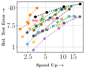
$\underbracket{\hskip 91.04872pt}_{\begin{subarray}{c}\vspace{-4.0mm}\\ \hbox{\pagecolor{white}(a) \scriptsize CIFAR100}\end{subarray}}$

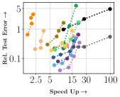
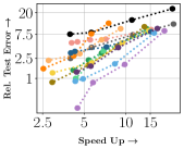
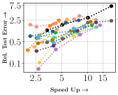
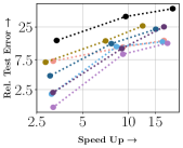
$\underbracket{\hskip 91.04872pt}_{\begin{subarray}{c}\vspace{-4.0mm}\\ \hbox{\pagecolor{white}(b) \scriptsize MNIST}\end{subarray}}$

$\underbracket{\hskip 91.04872pt}_{\begin{subarray}{c}\vspace{-4.0mm}\\ \hbox{\pagecolor{white}(c) \scriptsize CIFAR10}\end{subarray}}$

$\underbracket{\hskip 91.04872pt}_{\begin{subarray}{c}\vspace{-4.0mm}\\ \hbox{\pagecolor{white}(d) \scriptsize SVHN}\end{subarray}}$

$\underbracket{\hskip 91.04872pt}_{\begin{subarray}{c}\vspace{-4.0mm}\\ \hbox{\pagecolor{white}(e) \scriptsize ImageNet}\end{subarray}}$

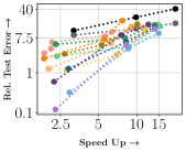
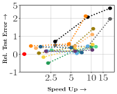
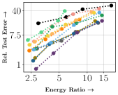
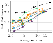
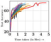
$\underbracket{\hskip 99.58464pt}_{\begin{subarray}{c}\vspace{-4.0mm}\\ \hbox{\pagecolor{white}(f) \scriptsize CIFAR10 Imbalance}\end{subarray}}$

$\underbracket{\hskip 99.58464pt}_{\begin{subarray}{c}\vspace{-4.0mm}\\ \hbox{\pagecolor{white}(g) \scriptsize MNIST Imbalance}\end{subarray}}$

$\underbracket{\hskip 99.58464pt}_{\begin{subarray}{c}\vspace{-4.0mm}\\ \hbox{\pagecolor{white}(h) \scriptsize CIFAR100 Energy}\end{subarray}}$

$\underbracket{\hskip 99.58464pt}_{\begin{subarray}{c}\vspace{-4.0mm}\\ \hbox{\pagecolor{white}(i) \scriptsize CIFAR10 Energy}\end{subarray}}$

$\underbracket{\hskip 99.58464pt}_{\begin{subarray}{c}\vspace{-4.0mm}\\ \hbox{\pagecolor{white}(j) \scriptsize CIFAR100 Convergence}\end{subarray}}$

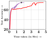
$\underbracket{\hskip 119.50148pt}_{\begin{subarray}{c}\vspace{-4.0mm}\\ \hbox{\pagecolor{white}(k) {\scriptsize CIFAR100 Ext. Convergence}}\end{subarray}}$

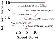
$\underbracket{\hskip 105.2751pt}_{\begin{subarray}{c}\vspace{-4.0mm}\\ \hbox{\pagecolor{white}(l) {\scriptsize CIFAR10 (MobileNet)}}\end{subarray}}$

Figure 3: Sub-figures (a-g) show speedup vs relative error in % tradeoff (both log-scale) of different algorithms. In each scatter plot, smaller subsets are on the left, and larger ones are on the right. Results are shown for (a) CIFAR-100, (b) MNIST, (c) CIFAR-10, (d) SVHN, (e) ImageNet, (f) CIFAR-10 imbalance, and (g) MNIST imbalance. Sub-figures (h, i) show energy gains vs. relative error for CIFAR-100 and CIFAR-10. Sub-figure (j) shows a convergence plot of different strategies at 30% subset of CIFAR-100. Sub-figure (k) shows an extended convergence plot of Grad-MatchPB-Warm at 30% subset of CIFAR-100 by running it for more epochs. Sub-figure (l) shows results of Grad-MatchPB-Warm using ResNet18 and Full training using MobileNet-V1 and MobileNet-V2 models on the CIFAR-10 dataset. In every case, the speedups & energy ratios are computed w.r.t full training. Variants of Grad-Match achieve best speedup-accuracy tradeoff (bottom-right in each scatter plot represents best speedup-accuracy tradeoff region) in almost all cases.

Warm-starting data selection: For each of the algorithms we consider in this paper (i.e., Grad-Match, Grad-MatchPB, Craig, CraigPB, and Glister), we also consider a warm-start variant, where we run $T_{f}$ epochs of full training. We set $T_{f}$ in a way such that the number of epochs $T_{s}$ with the subset of data is a fraction $\kappa$ of the total number of epochs, i.e., $T_{s}=\kappa T$ and $T_{f}=\frac{T_{s}k}{n}$, where $k$ is the subset size. We observe that doing full training for the first few epochs helps obtain good warm-start models, resulting in much better convergence. Setting $T_{f}$ to a large value yields results similar to the full training with early stopping (which we use as one of our baselines) since there is not enough data-selection.

Other speedups: We end this section by reiterating two implementation tricks already discussed in Section 3, namely, doing data selection every $R$ epochs (in our experiments, we set $R=20$, but also study the effect of the choice of $R$), and the per-batch (PB) versions of Craig and Grad-match.

5 Experiments

Our experiments aim to demonstrate the stability and efficiency of Grad-Match. While in most of our experiments, we study the tradeoffs between accuracy and efficiency (time/energy), we also study the robustness of data-selection under class imbalance. For most data selection experiments, we use the full loss gradients (i.e., $L=L_{T}$). As an exception, in the case of class imbalance, following (Killamsetty et al., 2021), we use $L=L_{V}$ (i.e., we assume access to a clean validation set).

Baselines in each setting. We compare the variants of our proposed algorithm (i.e., Grad-Match, Grad-MatchPB, Grad-Match-Warm, Grad-MatchPB-Warm) with variants of Craig (Mirzasoleiman et al., 2020a) (i.e., Craig, CraigPB, Craig-Warm, CraigPB-Warm), and variants of Glister (Killamsetty et al., 2021) (i.e., Glister, Glister-Warm). Additionally, we compare against Random (i.e., randomly select points equal to the budget), and Full-EarlyStop, where we do an early stop to full training to match the time taken (or energy used) by the subset selection.

Datasets, model architecture and experimental setup: To demonstrate the effectiveness of Grad-Match and its variants on real-world datasets, we performed experiments on CIFAR100 (60000 instances) (Krizhevsky, 2009), MNIST (70000 instances) (LeCun et al., 2010), CIFAR10 (60000 instances) (Krizhevsky, 2009), SVHN (99,289 instances) (Netzer et al., 2011), and ImageNet-2012 (1.4 Million instances) (Russakovsky et al., 2015) datasets. Wherever the datasets do not have a pre-specified validation set, we split the original training set into a new train (90%) and validation sets (10%). We ran experiments using an SGD optimizer with an initial learning rate of 0.01, a momentum of 0.9, and a weight decay of 5e-4. We decay the learning rate using cosine annealing (Loshchilov & Hutter, 2017) for each epoch. For MNIST, we use the LeNet model (LeCun et al., 1989) and train the model for 200 epochs. For all other datasets, we use the ResNet18 model (He et al., 2016) and train the model for 300 epochs (except for ImageNet, where we train the model for 350 epochs). In most of our experiments, we train the data selection algorithms (and full training) using the same number of epochs; the only difference is that each epoch is much smaller with smaller subsets, thereby enabling speedups/energy savings. We consider one additional experiment where we run Grad-MatchPB-Warm for $50$ more epochs to see how quickly it achieves comparable accuracy to full training. All experiments were run on V100 GPUs. Furthermore, the accuracies reported in the results are mean accuracies after five runs, and the standard deviations are given in Appendix C.5. More details are in Appendix C.

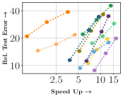
$\underbracket{\hskip 91.04872pt}_{\begin{subarray}{c}\vspace{-4.0mm}\\ \hbox{\pagecolor{white}(a) \scriptsize R analysis}\end{subarray}}$

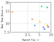
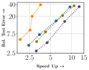
$\underbracket{\hskip 91.04872pt}_{\begin{subarray}{c}\vspace{-4.0mm}\\ \hbox{\pagecolor{white}(b) \scriptsize Optimal R}\end{subarray}}$

$\underbracket{\hskip 91.04872pt}_{\begin{subarray}{c}\vspace{-4.0mm}\\ \hbox{\pagecolor{white}(c) \scriptsize PB vs Non-PB}\end{subarray}}$

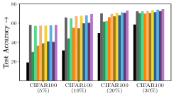
$\underbracket{\hskip 128.0374pt}_{\begin{subarray}{c}\vspace{-4.0mm}\\ \hbox{\pagecolor{white}(d) \scriptsize Warm vs Non-Warm}\end{subarray}}$

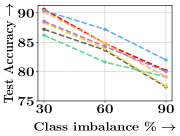
$\underbracket{\hskip 110.96556pt}_{\begin{subarray}{c}\vspace{-4.0mm}\\ \hbox{\pagecolor{white}(e) \scriptsize CIFAR10 Varying Imbalance}\end{subarray}}$

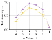
$\underbracket{\hskip 91.04872pt}_{\begin{subarray}{c}\vspace{-4.0mm}\\ \hbox{\pagecolor{white}(f) \scriptsize Kappa Analysis}\end{subarray}}$

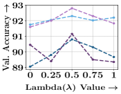
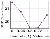
$\underbracket{\hskip 187.78836pt}_{\begin{subarray}{c}\vspace{-4.0mm}\\ \hbox{\pagecolor{white}\scriptsize(g) $\lambda$ Analysis(CIFAR10, 10\%)}\end{subarray}}$

Figure 4: Sub-figure (a) compares the effect of varying $R$ (5, 10 and 20) for different strategies (5% CIFAR-100). Sub-figure (b) compares $R=5$ with a 5% subset (circles) and $R=20$ with 10% subset (squares) showing that the latter is more efficient and accurate. Sub-figure (c) compares the per-batch (PB) versions with non-PB versions showing that the former has a better accuracy-efficiency trade-off. Sub-figure (d) compares the warm-start variants with the variants without warm-start for different subset sizes of CIFAR-100. Sub-figure (e) shows the performance of different selection strategies for 30% CIFAR-10 with varying percentages of imbalanced classes: 30%, 60%, and 90%. Grad-Match-Warm outperforms all baselines, including full training (which under-performs due to a high imbalance). Sub-figure (f) shows the effect of the warm-start parameter $\kappa$ for CIFAR-100. Sub-figure (g) shows the effect of the regularization parameter $\lambda$ on Grad-Match and its variants for 10% CIFAR-10.

Data selection setting: Since the goal of our experiments is efficiency, we use smaller subset sizes. For MNIST, we use sizes of [1%, 3%, 5%, 10%], for ImageNet-2012 we use [5%, 10%, 30%], while for the others, we use [5%, 10%, 20%, 30%]. For the warm versions, we set $\kappa=1/2$ (i.e. 50% warm-start and 50% data selection). Also, we set $R=20$ in all experiments. In our ablation study experiments, we study the effect of varying $R$ and $\kappa$.

Speedups and energy gains compared to full training: In Figures 3,3,3,3,3, we present scatter plots of relative error vs. speedups, both w.r.t full training. Figures 3,3 show scatter plots of relative error vs. energy efficiency, again w.r.t full training. In each case, we also include the cost of subset selection and subset training while computing the wall-clock time or energy consumed. For calculating the energy consumed by the GPU/CPU cores, we use pyJoules. As a first takeaway, we note that Grad-Match and its variants, achieve significant speedup (single GPU) and energy savings when compared to full training. In particular (c.f., Figure 1) for CIFAR-10, Grad-MatchPB-Warm achieves a 7x, 4.2x and 3x speedup and energy gains (with 10%, 20%, 30% subsets) with an accuracy drop of only 2.8%, 1.5% and 0.9% respectively. For CIFAR-100, Grad-MatchPB-Warm achieves a 4.8x and 3x speedup with an accuracy loss of 2.1% and 0.7% respectively, while for ImageNet, (30% subset), Grad-MatchPB-Warm achieves a 3x speedup with an accuracy loss of 1.3%. The gains are even more significant for MNIST.

Comparison to other baselines: Grad-MatchPB-Warm not only outperforms random selection and Full-EarlyStop consistently, but also outperforms variants of Craig, CraigPB, and Glister. Furthermore, Glister and Craig could not run on ImageNet due to large memory requirements and running time. Grad-Match, Grad-MatchPB, and CraigPB were the only variants which could scale to ImageNet. Furthermore, Glister and Craig also perform poorly on CIFAR-100. We see that Grad-MatchPB-Warm almost consistently achieves best speedup-accuracy tradeoff (i.e., the bottom right of the plots) on all datasets. We note that the performance gain provided by the variants of Grad-Match compared to other baselines like Glister, Craig and Full-EarlyStop is statistically significant (Wilcoxon signed-rank test (Wilcoxon, 1992) with a $p$ value $=0.01$). More details on the comparison (along with a detailed table of numbers) are in Appendix C.

Convergence and running time: Next, we compare the end-to-end training performance through a convergence plot. We plot test-accuracy versus training time in Figure 3. The plot shows that Grad-Match and specifically Grad-MatchPB-Warm is more efficient compared to other algorithms (including variants of Glister and Craig), and also converges faster than full training. Figure 3 shows the extended convergence of Grad-MatchPB-Warm on 30% CIFAR-100 subset, where the Grad-Match is allowed to train for as few more epochs to achieve comparable accuracy with Full training at the cost of losing some efficiency. The results show that Grad-MatchPB-Warm achieves similar performance to full training while being 2.5x faster, after running for just 30 to 50 additional epochs. Note that the points marked by * in Figure 3 denotes the standard training endpoint (i.e., 300 epochs) used for all experiments using CIFAR-100.

Comparison to smaller models: We compare the speedups achieved by Grad-Match to the speedups achieved using smaller models for training to understand the importance of data subset selection. We perform additional experiments (c.f., Figure. 3) on the CIFAR-10 dataset using MobileNet-V1 and MobileNet-V2 models as two proxies for small models. The results show that Grad-MatchPB-Warm outperforms the smaller models on both test accuracy and speedup (e.g., MobileNetV2 achieves less than 2x speedup with 1% accuracy drop).

Data selection with class imbalance: We check the robustness of Grad-Match and its variants for generalization by comparing the test accuracies achieved on a clean test dataset when class imbalance is present in the training dataset. Following (Killamsetty et al., 2021), we form a dataset by making 30% of the classes imbalanced by reducing the number of data points by 90%. We present results on CIFAR10 and MNIST in Figures 3,3 respectively. We use the (clean) validation loss for gradient matching in the class imbalance scenario since the training data is biased. The results show that Grad-Match and its variants outperform other baselines in all cases except for the 30% MNIST case (where Glister, which also uses a clean validation set, performs better). Furthermore, in the case of MNIST with imbalance, Grad-Match-warm even outperforms training on the entire dataset. Figure 4 shows the performance on 10% CIFAR-10 with varying percentages of imbalanced classes: 30% (as shown in Figure 3), 60% and 90%. Grad-Match-Warm outperforms all baselines, including full training (which under-performs due to a high imbalance). The trend is similar when we vary the degree of imbalance as well.

Ablation study results. Next, we study the effect of $R$, per-batch gradients, warm-start, $\lambda$, $\kappa$ and other hyper-parameters. We start with the effect of $R$ on the performance of Grad-Match and its variants. We study the result on CIFAR-100 dataset at 5% subset for varying values of $R$ (5,10,20) in the Figure 4 (with leftmost point corresponding to R=5 and the rightmost to R=20).The first takeaway is that, as expected, Grad-Match and its variants outperform other baselines for different R values. Secondly, this also helps us understand the accuracy-efficiency trade-off with different values of $R$. From Figure 4, we see that a 10% subset with $R=20$ yields accuracy similar to a 5% subset with $R=5$. However, across the different algorithms, we observe that $R=20$ is more efficient (from a time perspective) because of fewer subset selection runs. We then compare the PB variants of Craig and Grad-Match with their non-PB variants (c.f., Figure 4). We see that the PB versions are efficient and lie consistently to the bottom right (, i.e., lesser relative test accuracy and higher speedups) than non-PB counterparts. One of the main reasons for this is that the subset selection time for the PB variants is almost half that of the non-PB variant (c.f., Appendix C.4), with similar relative errors. Next, we study the effect of warm-start along with data selection. As shown in Figure 4, warm-start, in the beginning, helps the model come to a reasonable starting point for data selection, something which just random sets do not offer. We also observe that the effect of warm-start is more significant for smaller subset sizes (compared to larger sizes) in achieving large accuracy gains compared to the non-warm start versions. Figure 4 shows the effect of varying $\kappa$ (i.e., the warm-start fraction) for 10% of CIFAR-100. We observe that setting $\kappa=\frac{1}{2}$ generally performs the best. Setting a small value of $\kappa$ leads to sub-optimal performance because of not having a good starting point, while with larger values of $\kappa$ we do not have enough data selection and get results closer to the early stopping. The regularization parameter $\lambda$ prevents OMP from over-fitting (e.g., not assigning large weights to individual samples or mini-batches) since the subset selection is performed only every 20 epochs. Hence variants of Grad-Match performs poorly for small lambda values (e.g., $\lambda$=0) as shown in Figure. 4. Similarly, Grad-Match and its variants perform poorly for large $\lambda$ values as the OMP algorithm performs sub-optimally due to stronger restrictions on the possible sample weights. In our experiments, we found that $\lambda=0.5$ achieves the accuracy and efficiency (c.f., Figure. 4), and this holds consistently across subset sizes and datasets. Furthermore, we observed that $\epsilon$ does not significantly affect the performance of Grad-Match and its variants as long as $\epsilon$ is small (e.g., $\epsilon\leq 0.01$).

6 Conclusions

We introduce a Gradient Matching framework Grad-Match, which is inspired by the convergence analysis of adaptive data selection strategies. Grad-Match optimizes an error term, which measures how well the weighted subset matches either the full gradient or the validation set gradients. We study the algorithm’s theoretical properties (convergence rates and approximation bounds, connections to weak-submodularity) and finally demonstrate our algorithm’s efficacy by demonstrating that it achieves the best speedup-accuracy trade-off and is more energy-efficient through experiments on several datasets.

Appendix

Appendix A Summary of Notation

Topic	Notation	Explanation
	$U$	Set of $N$ instances in training set
Data (sub)Sets and indices	$V$	Set of $M$ instances in validation set
	$\mathcal{X}^{t}$	Subset of instances from $U$ at the $t^{th}$ epoch
	$W$	A generic reference to both $U$ and $V$
	$\pi_{t}^{i}\in\mathcal{X}$	Assignment of element $i\in W$ to an element of $\mathcal{X}$
	$\theta^{*}$	Optimal model parameter (vector)
Parameters	$\theta_{t}$	Updated parameter (vector) at the $t^{th}$ epoch
	$\mathbf{w}^{t}$	Vector weights associated with each data point in $\mathcal{X}^{t}$ (at the $t^{th}$ epoch)
Loss Functions	$L_{T}$	Training loss which when evaluated on $x_{i}\in U$ is referred to as $L_{T}^{i}$
	$L_{V}$	Validation loss which when evaluated on $x_{j}\in V$ is referred to as $L_{V}^{j}$
	$L$	Generic reference to the loss function which when evaluated on $x_{i}$ is referred to as $L^{i}$.
	$\mbox{Err}({\mathbf{w}}^{t},\mathcal{X}^{t},L,L_{T},\theta_{t})$	${\left\|\sum_{i\in\mathcal{X}^{t}}w^{t}_{i}\nabla_{\theta}L_{T}^{i}(\theta_{t})-\nabla_{\theta}L(\theta_{t})\right\|}$
	$E(\mathcal{X})$	$\min_{\mathbf{w}}\mbox{Err}(\mathbf{w},\mathcal{X},L,L_{T},\theta_{t})$
	$F(\mathcal{X})$	$L_{\max}-E(\mathcal{X})$ where $L_{\max}$ is an upperbound on $E(\mathcal{X})$
	$\hat{E}(\mathcal{X})$	The upper bound $\min_{\mathbf{w}}\mbox{Err}({\mathbf{w}},\mathcal{X},L,L_{T},\theta_{t})\leq\hat{E}(\mathcal{X})$ minimized in Section
	$\hat{F}(\mathcal{X})$	The facility location lower bound function $\sum_{i\in W}\max_{j\in\mathcal{X}}\big{(}L_{\max}-\|\nabla_{\theta}L^{i}(\theta_{t})-\nabla_{\theta}L_{T}^{j}(\theta_{t})\|\big{)}$ to be maximized
	$E_{\lambda}(\mathcal{X},\mathbf{w})$	Regularized version of $E(\mathcal{X})$ defined as $\big{\|}\sum_{i\in\mathcal{X}}{\mathbf{w}\nabla_{\theta}L_{T}^{i}(\theta)-\nabla_{\theta}L(\theta)\big{\|}^{2}+\lambda||{\mathbf{w}}||^{2}}$. See Section
	$E_{\lambda}(\mathcal{X})$	$\min_{{\mathbf{w}}}E_{\lambda}(\mathcal{X},\mathbf{w})$
	$F_{\lambda}(\mathcal{X})$	$L_{\max}-\min_{\mathbf{w}}E_{\lambda}(\mathcal{X},\mathbf{w})$ which we prove to be $\gamma$-weakly submodular in Section and subsequently maximize
	$\sigma_{T}$	Upperbound on the gradient of $L_{T}^{i}$
Hyperparameters	$\sigma_{V}$	Upperbound on the gradient of $L_{V}^{j}$
	$k$	Size of selected subset of points
	$R$	The number of training epochs after which data selection is periodically performed
	$\alpha_{t}$	The learning rate schedule at the $t^{th}$ epoch

Table 1: Organization of the notations used througout this paper

Appendix B Proofs of the Technical Results

B.1 Proof of Theorem 1

We begin by first stating and then proving Theorem 1.

Theorem.

Any adaptive data selection algorithm (run with full gradient descent), defined via weights $\mathbf{w}^{t}$ and subsets $\mathcal{X}^{t}$ for $t=1,\cdots,T$, enjoys the following guarantees:
(1). If $L_{T}$ is Lipschitz continuous with parameter $\sigma_{T}$, optimal model parameters $\theta^{*}$, and $\alpha=\frac{D}{\sigma_{T}\sqrt{T}}$, then $\min_{t=1:T}L(\theta_{t})-L(\theta^{*})\leq\frac{D\sigma_{T}}{\sqrt{T}}+\frac{D}{T}\sum_{t=1}^{T-1}\mbox{Err}(\mathbf{w}^{t},\mathcal{X}^{t},L,L_{T},\theta_{t})$.
(2) If $L_{T}$ is Lipschitz smooth with parameter $\mathcal{L}_{T}$, optimal model parameters $\theta^{*}$, and $L_{T}^{i}$ satisfies $0\leq L_{T}^{i}(\theta)\leq\beta_{T}$, $\forall i$, then setting $\alpha=\frac{1}{\mathcal{L}_{T}}$, we have $\min_{t=1:T}L(\theta_{t})-L(\theta^{*})\leq\frac{D^{2}\mathcal{L}_{T}+2\beta_{T}}{2T}+\frac{D}{T}\sum_{t=1}^{T-1}\mbox{Err}(\mathbf{w}^{t},\mathcal{X}^{t},L,L_{T},\theta_{t})$.
(3) If $L_{T}$ is Lipschitz continuous with parameter $\sigma_{T}$, optimal model parameters $\theta^{*}$, and $L$ is strongly convex with parameter $\mu$, then setting a learning rate $\alpha_{t}=\frac{2}{\mu(1+t)}$, we have $\min_{t=1:T}L(\theta_{t})-L(\theta^{*})\leq\frac{2{\sigma_{T}}^{2}}{\mu(T+1)}+\sum_{t=1}^{t=T}\frac{2Dt}{T(T+1)}\mbox{Err}(\mathbf{w}^{t},\mathcal{X}^{t},L,L_{T},\theta_{t})$.

Proof.

Suppose the gradients of validation loss and training loss are sigma bounded by $\sigma_{V}$ and $\sigma_{T}$ respectively. Let $\theta_{t}$ be the model parameters at epoch $t$ and $\theta^{*}$ be the optimal model parameters.

Let, $L_{w}(\theta_{t})=\underset{i\in\mathcal{X}^{t}}{\sum}w^{t}_{i}L_{T}^{i}(\theta_{t})$ be the weighted subset training loss parameterized by model parameters $\theta_{t}$ at time step t. Let $\alpha_{t}$ be the learning rate used at epoch $t$.

From the definition of Gradient Descent, we have:

$${\nabla_{\theta}L_{w}(\theta_{t})}^{T}(\theta_{t}-\theta^{*})=\frac{1}{\alpha_{t}}{(\theta_{t}-\theta_{t+1})}^{T}(\theta_{t}-\theta^{*})$$ (6)

$${\nabla_{\theta}L_{w}(\theta_{t})}^{T}(\theta_{t}-\theta^{*})=\frac{1}{2\alpha_{t}}\left({\left\|\theta_{t}-\theta_{t+1}\right\|}^{2}+{\left\|\theta_{t}-\theta^{*}\right\|}^{2}-{\left\|\theta_{t+1}-\theta^{*}\right\|}^{2}\right)$$ (7)

$${\nabla_{\theta}L_{w}(\theta_{t})}^{T}(\theta_{t}-\theta^{*})=\frac{1}{2\alpha_{t}}\left({\left\|\alpha_{t}\sum_{i\in\mathcal{X}^{t}}w^{t}_{i}\nabla_{\theta}L_{T}^{i}(\theta_{t})\right\|}^{2}+{\left\|\theta_{t}-\theta^{*}\right\|}^{2}-{\left\|\theta_{t+1}-\theta^{*}\right\|}^{2}\right)$$ (8)

We can rewrite the function ${\nabla_{\theta}L_{w}(\theta_{t})}^{T}(\theta_{t}-\theta^{*})$ as follows:

$${\nabla_{\theta}L_{w}(\theta_{t})}^{T}(\theta_{t}-\theta^{*})={\nabla_{\theta}L_{w}(\theta_{t})}^{T}(\theta_{t}-\theta^{*})-{\nabla_{\theta}L(\theta_{t})}^{T}(\theta_{t}-\theta^{*})+{\nabla_{\theta}L(\theta_{t})}^{T}(\theta_{t}-\theta^{*})$$ (9)

Combining the equations (8) and (9) we have,

$${\nabla_{\theta}L_{w}(\theta_{t})}^{T}(\theta_{t}-\theta^{*})-{\nabla_{\theta}L(\theta_{t})}^{T}(\theta_{t}-\theta^{*})+{\nabla_{\theta}L(\theta_{t})}^{T}(\theta_{t}-\theta^{*})=\frac{1}{2\alpha_{t}}\left({\left\|\alpha_{t}\sum_{i\in\mathcal{X}^{t}}w^{t}_{i}\nabla_{\theta}L_{T}^{i}(\theta_{t})\right\|}^{2}+{\left\|\theta_{t}-\theta^{*}\right\|}^{2}-{\left\|\theta_{t+1}-\theta^{*}\right\|}^{2}\right)$$ (10)

$${\nabla_{\theta}L(\theta_{t})}^{T}(\theta_{t}-\theta^{*})=\frac{1}{2\alpha_{t}}\left({\left\|\alpha_{t}\sum_{i\in\mathcal{X}^{t}}w^{t}_{i}\nabla_{\theta}L_{T}^{i}(\theta_{t})\right\|}^{2}+{\left\|\theta_{t}-\theta^{*}\right\|}^{2}-{\left\|\theta_{t+1}-\theta^{*}\right\|}^{2}\right)-{\left(\nabla_{\theta}L_{w}(\theta_{t})-\nabla_{\theta}L(\theta_{t})\right)}^{T}(\theta_{t}-\theta^{*})$$ (11)

Summing up equation (11) for different values of $t\in[0,T-1]$ and assuming a constant learning rate of $\alpha_{t}=\alpha$, we have:

$$\sum_{t=0}^{T-1}{\nabla_{\theta}L(\theta_{t})}^{T}(\theta_{t}-\theta^{*})= \frac{1}{2\alpha}{\left\|\theta_{0}-\theta^{*}\right\|}^{2}-{\left\|\theta_{T}-\theta^{*}\right\|}^{2}+\sum_{t=0}^{T-1}(\frac{1}{2\alpha}{\left\|\alpha\sum_{i\in\mathcal{X}^{t}}w^{t}_{i}\nabla_{\theta}L_{T}^{i}(\theta_{t})\right\|}^{2})$$

$$+\sum_{t=0}^{T-1}\left({\left(\nabla_{\theta}L_{w}(\theta_{t})-\nabla_{\theta}L(\theta_{t})\right)}^{T}(\theta_{t}-\theta^{*})\right)$$

Since ${\left\|\theta_{T}-\theta^{*}\right\|}^{2}\geq 0$, we have:

$$\sum_{t=0}^{T-1}{\nabla_{\theta}L(\theta_{t})}^{T}(\theta_{t}-\theta^{*})\leq\frac{1}{2\alpha}{\left\|\theta_{0}-\theta^{*}\right\|}^{2}+\sum_{t=0}^{T-1}(\frac{1}{2\alpha}{\left\|\alpha\sum_{i\in\mathcal{X}^{t}}w^{t}_{i}\nabla_{\theta}L_{T}^{i}(\theta_{t})\right\|}^{2})+\sum_{t=0}^{T-1}\left({\left(\nabla_{\theta}L_{w}(\theta_{t})-\nabla_{\theta}L(\theta_{t})\right)}^{T}(\theta_{t}-\theta^{*})\right)$$ (12)

Case 1.

$L_{T}$ is lipschitz continuous with parameter $\sigma_{T}$ and $L$ is a convex function

From convexity of function $L(\theta)$, we know $L(\theta_{t})-L(\theta^{*})\leq{\nabla_{\theta}L(\theta_{t})}^{T}(\theta_{t}-\theta^{*})$. Combining this with Equation 12 we have,

$$\sum_{t=0}^{T-1}L(\theta_{t})-L(\theta^{*})\leq\frac{1}{2\alpha}{\left\|\theta_{0}-\theta^{*}\right\|}^{2}+\sum_{t=0}^{T-1}(\frac{1}{2\alpha}{\left\|\alpha\sum_{i\in\mathcal{X}^{t}}w^{t}_{i}\nabla_{\theta}L_{T}^{i}(\theta_{t})\right\|}^{2})+\sum_{t=0}^{T-1}\left({\left(\nabla_{\theta}L_{w}(\theta_{t})-\nabla_{\theta}L(\theta_{t})\right)}^{T}(\theta_{t}-\theta^{*})\right)$$ (13)

Since, $\left\|L_{T}(\theta)\right\|\leq\sigma_{T}$, we have ${\left\|\alpha\sum_{i\in\mathcal{X}^{t}}w^{t}_{i}\nabla_{\theta}L_{T}^{i}(\theta_{t})\right\|}\leq\sum_{i=1}^{|\mathcal{X}^{t}|}w_{i}^{t}\sigma$. Assuming that the weights at every iteration are normalized such that $\underset{t\in[1,T]}{\forall}\sum_{i=1}^{|\mathcal{X}^{t}|}w_{i}^{t}=1$ and the training and validation loss gradients are normalized as well, we have ${\left\|\alpha\sum_{i\in\mathcal{X}^{t}}w^{t}_{i}\nabla_{\theta}L_{T}^{i}(\theta_{t})\right\|}\leq\sigma_{T}$. Also assuming that $\left\|\theta-\theta^{*}\right\|\leq D$, we have,

$$\sum_{t=0}^{T-1}L(\theta_{t})-L(\theta^{*})\leq\frac{D^{2}}{2\alpha}+\frac{T\alpha\sigma_{T}^{2}}{2}+\sum_{t=0}^{T-1}D\left({\left\|\nabla_{\theta}L_{w}(\theta_{t})-\nabla_{\theta}L(\theta_{t})\right\|}\right)$$ (14)

$$\frac{\sum_{t=0}^{T-1}L(\theta_{t})-L(\theta^{*})}{T}\leq\frac{D^{2}}{2\alpha T}+\frac{\alpha\sigma_{T}^{2}}{2}+\sum_{t=0}^{T-1}\frac{D}{T}\left({\left\|\nabla_{\theta}L_{w}(\theta_{t})-\nabla_{\theta}L(\theta_{t})\right\|}\right)$$ (15)

Since, $\min{(L(\theta_{t})-L(\theta^{*}))}\leq\frac{\sum_{t=0}^{T-1}L(\theta_{t})-L(\theta^{*})}{T}$, we have:

$$\min{(L(\theta_{t})-L(\theta^{*}))}\leq\frac{D^{2}}{2\alpha T}+\frac{\alpha\sigma_{T}^{2}}{2}+\sum_{t=0}^{T-1}\frac{D}{T}\left({\left\|\nabla_{\theta}L_{w}(\theta_{t})-\nabla_{\theta}L(\theta_{t})\right\|}\right)$$ (16)

Substituting $L_{w}(\theta_{t})=\underset{i\in\mathcal{X}^{t}}{\sum}w^{t}_{i}L_{T}^{i}(\theta_{t})$ in the above equation we have,

$$\min{(L(\theta_{t})-L(\theta^{*}))}\leq\frac{D^{2}}{2\alpha T}+\frac{\alpha\sigma_{T}^{2}}{2}+\sum_{t=0}^{T-1}\frac{D}{T}\left({\left\|\underset{i\in\mathcal{X}^{t}}{\sum}w^{t}_{i}\nabla_{\theta}L_{T}^{i}(\theta_{t})-\nabla_{\theta}L(\theta_{t})\right\|}\right)$$ (17)

Choosing $\alpha=\frac{D}{\sigma_{T}\sqrt{T}}$, we have:

$$\min{(L(\theta_{t})-L(\theta^{*}))}\leq\frac{D\sigma_{T}}{\sqrt{T}}+\sum_{t=0}^{T-1}\frac{D}{T}\left({\left\|\underset{i\in\mathcal{X}^{t}}{\sum}w^{t}_{i}\nabla_{\theta}L_{T}^{i}(\theta_{t})-\nabla_{\theta}L(\theta_{t})\right\|}\right)$$ (18)

Case 2.

$L_{T}$ is lipschitz smooth with parameter $\mathcal{L}_{T}$, and $\forall i$, $L_{T}^{i}$ satisfies $0\leq L_{T}^{i}(\theta)\leq\beta_{T}$

Since $L_{w}(\theta_{t})=\underset{i\in\mathcal{X}^{t}}{\sum}w^{t}_{i}L_{T}^{i}(\theta_{t})$, from the additive property of lipschitz smooth functions we can say that $L_{w}(\theta_{t})$ is also lipschitz smooth with constant $\underset{i\in\mathcal{X}^{t}}{\sum}w^{t}_{i}\mathcal{L}_{T}$. Assuming that the weights at every iteration are normalized such that $\underset{t\in[0,T]}{\forall}\sum_{i=1}^{|\mathcal{X}^{t}|}w_{i}^{t}=1$, we can say that $L_{w}(\theta_{t})$ is lipschitz smooth with constant $\mathcal{L}_{T}$.

From lipschitz smoothness of function $L_{w}(\theta)$, we have:

$$L_{w}(\theta_{t+1})\leq L_{w}(\theta_{t})+\nabla_{\theta}L_{w}(\theta_{t})^{T}(\theta_{t+1}-\theta_{t})+\frac{L}{2}{\left\|\theta_{t+1}-\theta_{t}\right\|}^{2}$$ (19)

Since $\theta_{t+1}-\theta_{t}=-\alpha\nabla_{\theta}L_{w}(\theta_{t})$, we have:

$$L_{w}(\theta_{t+1})\leq L_{w}(\theta_{t})-\alpha\nabla_{\theta}L_{w}(\theta_{t})^{T}\nabla_{\theta}L_{w}(\theta_{t})+\frac{\mathcal{L}_{T}}{2}{\left\|\alpha\nabla_{\theta}L_{w}(\theta_{t})\right\|}^{2}$$ (20)

$$L_{w}(\theta_{t+1})\leq L_{w}(\theta_{t})+\frac{\mathcal{L}_{T}\alpha^{2}-2\alpha}{2}{\left\|\nabla_{\theta}L_{w}(\theta_{t})\right\|}^{2}$$ (21)

Choosing $\alpha=\frac{1}{\mathcal{L}_{T}}$, we have:

$$L_{w}(\theta_{t+1})\leq L_{w}(\theta_{t})-\frac{1}{2\mathcal{L}_{T}}{\left\|\nabla_{\theta}L_{w}(\theta_{t})\right\|}^{2}$$ (22)

Since $\nabla_{\theta}L_{w}(\theta_{T})=\underset{i\in\mathcal{X}^{t}}{\sum}w^{t}_{i}\nabla_{\theta}L_{T}^{i}(\theta_{t})$, we have:

$$L_{w}(\theta_{t+1})\leq L_{w}(\theta_{t})-\frac{1}{2\mathcal{L}_{T}}{\left\|\underset{i\in\mathcal{X}^{t}}{\sum}w^{t}_{i}\nabla_{\theta}L_{T}^{i}(\theta_{t})\right\|}^{2}$$ (23)

$$\frac{1}{2\mathcal{L}_{T}}{\left\|\underset{i\in\mathcal{X}^{t}}{\sum}w^{t}_{i}\nabla_{\theta}L_{T}^{i}(\theta_{t})\right\|}^{2}\leq L_{w}(\theta_{t})-L_{w}(\theta_{t+1})$$ (24)

Summing the above equation for different values of $t$ in $[0,T-1]$, we have:

$$\sum_{t=0}^{t=T-1}\frac{1}{2\mathcal{L}_{T}}{\left\|\underset{i\in\mathcal{X}^{t}}{\sum}w^{t}_{i}\nabla_{\theta}L_{T}^{i}(\theta_{t})\right\|}^{2}\leq\sum_{t=0}^{t=T-1}(L_{w}(\theta_{t})-L_{w}(\theta_{t+1}))$$ (25)

$$\sum_{t=0}^{t=T-1}\frac{1}{2\mathcal{L}_{T}}{\left\|\underset{i\in\mathcal{X}^{t}}{\sum}w^{t}_{i}\nabla_{\theta}L_{T}^{i}(\theta_{t})\right\|}^{2}\leq L_{w}(\theta_{0})-L_{w}(\theta_{T})$$ (26)

Substituting $\alpha=\frac{1}{\mathcal{L}_{T}}$ in Equation 12, we have:

$$\sum_{t=0}^{T-1}{\nabla_{\theta}L(\theta_{t})}^{T}(\theta_{t}-\theta^{*})\leq\frac{\mathcal{L}_{T}}{2}{\left\|\theta_{0}-\theta^{*}\right\|}^{2}+\sum_{t=0}^{T-1}(\frac{1}{2\mathcal{L}_{T}}{\left\|\sum_{i\in\mathcal{X}^{t}}w^{t}_{i}\nabla_{\theta}L_{T}^{i}(\theta_{t})\right\|}^{2})+\sum_{t=0}^{T-1}\left({\left(\nabla_{\theta}L_{w}(\theta_{t})-\nabla_{\theta}L(\theta_{t})\right)}^{T}(\theta_{t}-\theta^{*})\right)$$ (27)

Substituting Equation 26, we have:

$$\sum_{t=0}^{T-1}{\nabla_{\theta}L(\theta_{t})}^{T}(\theta_{t}-\theta^{*})\leq\frac{\mathcal{L}_{T}}{2}{\left\|\theta_{0}-\theta^{*}\right\|}^{2}+L_{w}(\theta_{0})-L_{w}(\theta_{T})+\sum_{t=0}^{T-1}\left({\left(\nabla_{\theta}L_{w}(\theta_{t})-\nabla_{\theta}L(\theta_{t})\right)}^{T}(\theta_{t}-\theta^{*})\right)$$ (28)

$$\sum_{t=0}^{T-1}{\nabla_{\theta}L(\theta_{t})}^{T}(\theta_{t}-\theta^{*})\leq\frac{\mathcal{L}_{T}}{2}{\left\|\theta_{0}-\theta^{*}\right\|}^{2}+L_{w}(\theta_{0})+\sum_{t=0}^{T-1}\left({\left(\nabla_{\theta}L_{w}(\theta_{t})-\nabla_{\theta}L(\theta_{t})\right)}^{T}(\theta_{t}-\theta^{*})\right)$$ (29)

Since $L_{T}(\theta)$ is bounded by $\beta_{T}$, we have $L_{w}(\theta)=\underset{i\in\mathcal{X}^{t}}{\sum}w^{t}_{i}L_{T}^{i}(\theta)$ bounded by $\beta_{T}$ as the weights are normalized to $1$ every epoch (i.e., $\underset{t\in[0,T]}{\forall}\sum_{i=1}^{|\mathcal{X}^{t}|}w_{i}^{t}=1$).

$$\sum_{t=0}^{T-1}{\nabla_{\theta}L(\theta_{t})}^{T}(\theta_{t}-\theta^{*})\leq\frac{\mathcal{L}_{T}}{2}{\left\|\theta_{0}-\theta^{*}\right\|}^{2}+\beta_{T}+\sum_{t=0}^{T-1}\left({\left(\nabla_{\theta}L_{w}(\theta_{t})-\nabla_{\theta}L(\theta_{t})\right)}^{T}(\theta_{t}-\theta^{*})\right)$$ (30)

Dividing the above equation by T, we have:

$$\frac{\sum_{t=0}^{T-1}{\nabla_{\theta}L(\theta_{t})}^{T}(\theta_{t}-\theta^{*})}{T}\leq\frac{\mathcal{L}_{T}}{2T}{\left\|\theta_{0}-\theta^{*}\right\|}^{2}+\frac{\beta_{T}}{T}+\frac{\sum_{t=0}^{T-1}\left({\left(\nabla_{\theta}L_{w}(\theta_{t})-\nabla_{\theta}L(\theta_{t})\right)}^{T}(\theta_{t}-\theta^{*})\right)}{T}$$ (31)

Since $\left\|\theta-\theta^{*}\right\|\leq D$, we have,

$$\frac{\sum_{t=0}^{T-1}{\nabla_{\theta}L(\theta_{t})}^{T}(\theta_{t}-\theta^{*})}{T}\leq\frac{D^{2}\mathcal{L}_{T}}{2T}+\frac{\beta_{T}}{T}+\frac{D}{T}\sum_{t=0}^{T-1}\left({\left\|\nabla_{\theta}L_{w}(\theta_{t})-\nabla_{\theta}L(\theta_{t})\right\|}\right)$$ (32)

From convexity of function $L(\theta)$, we know $L(\theta_{t})-L(\theta^{*})\leq{\nabla_{\theta}L(\theta_{t})}^{T}(\theta_{t}-\theta^{*})$. Combining this with above equation we have,

$$\frac{\sum_{t=0}^{T-1}L(\theta_{t})-L(\theta^{*})}{T}\leq\frac{D^{2}\mathcal{L}_{T}}{2T}+\frac{\beta_{T}}{T}+\frac{D}{T}\sum_{t=0}^{T-1}\left({\left\|\nabla_{\theta}L_{w}(\theta_{t})-\nabla_{\theta}L(\theta_{t})\right\|}\right)$$ (33)

Since, $\min{(L(\theta_{t})-L(\theta^{*}))}\leq\frac{\sum_{t=0}^{T-1}L(\theta_{t})-L(\theta^{*})}{T}$, we have:

$$\min{(L(\theta_{t})-L(\theta^{*}))}\leq\frac{D^{2}\mathcal{L}_{T}}{2T}+\frac{\beta_{T}}{T}+\frac{D}{T}\sum_{t=0}^{T-1}\left({\left\|\nabla_{\theta}L_{w}(\theta_{t})-\nabla_{\theta}L(\theta_{t})\right\|}\right)$$ (34)

Substituting $L_{w}(\theta_{t})=\underset{i\in\mathcal{X}^{t}}{\sum}w^{t}_{i}L_{T}^{i}(\theta_{t})$ in the above equation we have,

$$\min{(L(\theta_{t})-L(\theta^{*}))}\leq\frac{D^{2}\mathcal{L}_{T}}{2T}+\frac{\beta_{T}}{T}+\frac{D}{T}\sum_{t=0}^{T-1}\left({\left\|\underset{i\in\mathcal{X}^{t}}{\sum}w^{t}_{i}\nabla_{\theta}L_{T}^{i}(\theta_{t})-\nabla_{\theta}L(\theta_{t})\right\|}\right)$$ (35)

Case 3.

$L_{T}$ is Lipschitz continuous (parameter $\sigma_{T}$) and $L$ is strongly convex with parameter $\mu$

Let the learning at time step $t$ be $\alpha_{t}$

From Equation 11, we have:

$${\nabla_{\theta}L(\theta_{t})}^{T}(\theta_{t}-\theta^{*})=\frac{1}{2\alpha_{t}}\left({\left\|\alpha_{t}\sum_{i\in\mathcal{X}^{t}}w^{t}_{i}\nabla_{\theta}L_{T}^{i}(\theta_{t})\right\|}^{2}+{\left\|\theta_{t}-\theta^{*}\right\|}^{2}-{\left\|\theta_{t+1}-\theta^{*}\right\|}^{2}\right)-{\left(\nabla_{\theta}L_{w}(\theta_{t})-\nabla_{\theta}L(\theta_{t})\right)}^{T}(\theta_{t}-\theta^{*})$$ (36)

From the strong convexity of loss function $L$, we have:

$$\nabla_{\theta}L(\theta_{t})^{T}(\theta_{t}-\theta^{*})\geq L(\theta_{t})-L(\theta^{*})+\frac{\mu}{2}{\left\|\theta_{t}-\theta^{*}\right\|}^{2}$$ (37)

Combining the above two equations, we have:

$$L(\theta_{t})-L(\theta^{*})=\frac{1}{2\alpha_{t}}\left({\left\|\alpha_{t}\sum_{i\in\mathcal{X}^{t}}w^{t}_{i}\nabla_{\theta}L_{T}^{i}(\theta_{t})\right\|}^{2}+{\left\|\theta_{t}-\theta^{*}\right\|}^{2}-{\left\|\theta_{t+1}-\theta^{*}\right\|}^{2}\right)-{\left(\nabla_{\theta}L_{w}(\theta_{t})-\nabla_{\theta}L(\theta_{t})\right)}^{T}(\theta_{t}-\theta^{*})-\frac{\mu}{2}{\left\|\theta_{t}-\theta^{*}\right\|}^{2}$$ (38)

$$L(\theta_{t})-L(\theta^{*})=\frac{\alpha_{t}}{2}{\left\|\sum_{i\in\mathcal{X}^{t}}w^{t}_{i}\nabla_{\theta}L_{T}^{i}(\theta_{t})\right\|}^{2}+\frac{\alpha_{t}^{-1}-\mu}{2}{\left\|\theta_{t}-\theta^{*}\right\|}^{2}-\frac{\alpha_{t}^{-1}}{2}{\left\|\theta_{t+1}-\theta^{*}\right\|}^{2}-{\left(\nabla_{\theta}L_{w}(\theta_{t})-\nabla_{\theta}L(\theta_{t})\right)}^{T}(\theta_{t}-\theta^{*})$$ (39)

Setting an learning rate of $\alpha_{t}=\frac{2}{\mu(t+1)}$ and multiplying by $t$ on both sides, we have:

$$t(L(\theta_{t})-L(\theta^{*})) =\frac{t}{\mu(t+1)}{\left\|\sum_{i\in\mathcal{X}^{t}}w^{t}_{i}\nabla_{\theta}L_{T}^{i}(\theta_{t})\right\|}^{2}+\frac{\mu t(t-1)}{4}{\left\|\theta_{t}-\theta^{*}\right\|}^{2}$$ (40)

$$-\frac{\mu t(t+1)}{4}{\left\|\theta_{t+1}-\theta^{*}\right\|}^{2}-t{\left(\nabla_{\theta}L_{w}(\theta_{t})-\nabla_{\theta}L(\theta_{t})\right)}^{T}(\theta_{t}-\theta^{*})$$

Since, $\left\|L_{T}(\theta)\right\|\leq\sigma_{T}$, we have ${\left\|\alpha\sum_{i\in\mathcal{X}^{t}}w^{t}_{i}\nabla_{\theta}L_{T}^{i}(\theta_{t})\right\|}\leq\sum_{i=1}^{|\mathcal{X}^{t}|}w_{i}^{t}\sigma_{T}$. Assuming that the weights at every iteration are normalized such that $\underset{t\in[1,T]}{\forall}\sum_{i=1}^{|\mathcal{X}^{t}|}w_{i}^{t}=1$ and the training and validation loss gradients are normalized as well, we have ${\left\|\alpha\sum_{i\in\mathcal{X}^{t}}w^{t}_{i}\nabla_{\theta}L_{T}^{i}(\theta_{t})\right\|}\leq\sigma_{T}$. Also assuming that $\left\|\theta-\theta^{*}\right\|\leq D$, we have,

$$t(L(\theta_{t})-L(\theta^{*})) =\frac{{\sigma_{T}}^{2}t}{\mu(t+1)}+\frac{\mu t(t-1)}{4}{\left\|\theta_{t}-\theta^{*}\right\|}^{2}$$ (41)

$$-\frac{\mu t(t+1)}{4}{\left\|\theta_{t+1}-\theta^{*}\right\|}^{2}+Dt\left\|\nabla_{\theta}L_{w}(\theta_{t})-\nabla_{\theta}L(\theta_{t})\right\|$$

Summing the above equation from $t=1,\cdots,T$, we have:

$$\sum_{t=1}^{t=T}t(L(\theta_{t})-L(\theta^{*})) =\sum_{t=1}^{t=T}\frac{{\sigma_{T}}^{2}t}{\mu(t+1)}+\sum_{t=1}^{t=T}\frac{\mu t(t-1)}{4}{\left\|\theta_{t}-\theta^{*}\right\|}^{2}$$ (42)

$$-\sum_{t=1}^{t=T}\frac{\mu t(t+1)}{4}{\left\|\theta_{t+1}-\theta^{*}\right\|}^{2}+\sum_{t=1}^{t=T}Dt\left\|\nabla_{\theta}L_{w}(\theta_{t})-\nabla_{\theta}L(\theta_{t})\right\|$$

$$\sum_{t=1}^{t=T}t(L(\theta_{t})-L(\theta^{*})) \leq\sum_{t=1}^{t=T}\frac{{\sigma_{T}}^{2}}{\mu}+\sum_{t=1}^{t=T}\frac{\mu t(t-1)}{4}{\left\|\theta_{t}-\theta^{*}\right\|}^{2}$$ (43)

$$-\sum_{t=1}^{t=T}\frac{\mu t(t+1)}{4}{\left\|\theta_{t+1}-\theta^{*}\right\|}^{2}+\sum_{t=1}^{t=T}Dt\left\|\nabla_{\theta}L_{w}(\theta_{t})-\nabla_{\theta}L(\theta_{t})\right\|$$

$$\sum_{t=1}^{t=T}t(L(\theta_{t})-L(\theta^{*})) \leq\frac{{\sigma_{T}}^{2}T}{\mu}+\frac{\mu}{4}(0-T(T+1){\left\|\theta_{T+1}-\theta^{*}\right\|}^{2})$$ (44)

$$+\sum_{t=1}^{t=T}Dt\left\|\nabla_{\theta}L_{w}(\theta_{t})-\nabla_{\theta}L(\theta_{t})\right\|$$

Since $\frac{\mu}{4}(0-T(T+1){\left\|\theta_{T+1}-\theta^{*}\right\|}^{2})\leq 0$, we have:

$$\sum_{t=1}^{t=T}t(L(\theta_{t})-L(\theta^{*})) \leq\frac{{\sigma_{T}}^{2}T}{\mu}+\sum_{t=1}^{t=T}Dt\left\|\nabla_{\theta}L_{w}(\theta_{t})-\nabla_{\theta}L(\theta_{t})\right\|$$ (45)

Since, $L(\theta_{t})-L(\theta^{*})\leq\min_{t=1:T}L(\theta_{t})-L(\theta^{*})$ and multiplying the above equation by $\frac{2}{T(T+1)}$, we have:

$$\frac{2}{T(T+1)}\sum_{t=1}^{t=T}t(\min_{t=1:T}L(\theta_{t})-L(\theta^{*}))\leq\frac{2}{T(T+1)}\frac{{\sigma_{T}}^{2}T}{\mu}+\frac{2}{T(T+1)}\sum_{t=1}^{t=T}Dt\left\|\nabla_{\theta}L_{w}(\theta_{t})-\nabla_{\theta}L(\theta_{t})\right\|$$ (46)

This in turn implies:

$$\min_{t=1:T}L(\theta_{t})-L(\theta^{*}) \leq\frac{{\sigma_{T}}^{2}2}{\mu(T+1)}+\sum_{t=1}^{t=T}\frac{2Dt}{T(T+1)}\left\|\nabla_{\theta}L_{w}(\theta_{t})-\nabla_{\theta}L(\theta_{t})\right\|$$ (47)

B.2 Convergence Analysis with Stochastic Gradient Descent

Theorem.

Denote $L_{V}$ as the validation loss, $L_{T}$ as the full training loss, and that the parameters satisfy $||\theta||^{2}\leq D^{2}$. Let $L$ denote either the training or validation loss (with gradient bounded by $\sigma$). Any adaptive data selection algorithm, defined via weights $\mathbf{w}^{t}$ and subsets $\mathcal{X}^{t}$ for $t=1,\cdots,T$, and run with a learning rate $\alpha$ using stochastic gradient descent enjoys the following convergence bounds:

• if $L_{T}$ is lipschitz continuous and $\alpha=\frac{D}{\sigma_{T}\sqrt{T}}$, then $\mathop{\mathbb{E}}\left(\min_{t=1:T}L(\theta_{t})\right)-L(\theta^{*})\leq\frac{D\sigma_{T}}{\sqrt{T}}+\frac{D}{T}\sum_{t=1}^{T-1}\mathop{\mathbb{E}}(\mbox{Err}(\mathbf{w}^{t},\mathcal{X}^{t},L,L_{T},\theta_{t}))$

• if $L_{T}$ is Lipschitz continuous, $L$ is strongly convex with a strong convexity parameter $\mu$, then setting a learning rate $\alpha_{t}=\frac{2}{\mu(1+t)}$, then $\mathop{\mathbb{E}}\left(\min_{t=1:T}L(\theta_{t})\right)-L(\theta^{*})\leq\frac{{\sigma_{T}}^{2}2}{\mu(T+1)}+\sum_{t=1}^{t=T}\frac{2D}{T(T+1)}\mathop{\mathbb{E}}\left(t\mbox{Err}(\mathbf{w}^{t},\mathcal{X}^{t},L,L_{T},\theta_{t})\right)$

where:
$\mbox{Err}(\mathbf{w}^{t},\mathcal{X}^{t},L,L_{T},\theta_{t})={\left\|\sum_{i\in\mathcal{X}^{t}}w^{t}_{i}\nabla_{\theta}L_{T}^{i}(\theta_{t})-\nabla_{\theta}L(\theta_{t})\right\|}$

Proof.

Suppose the gradients of validation loss and training loss are sigma bounded by $\sigma_{V}$ and $\sigma_{T}$ respectively. Let $\theta_{t}$ be the model parameters at epoch $t$ and $\theta^{*}$ be the optimal model parameters. Let $\alpha_{t}$ is the learning rate at epoch $t$.

Let $L_{w}(\theta_{t})=\underset{i\in\mathcal{X}^{t}}{\sum}w^{t}_{i}L_{T}^{i}(\theta_{t})$ be the weighted training loss where $L_{T}^{i}(\theta_{t})$ is the training loss of the $i^{th}$ instance in the subset $\mathcal{X}^{t}$.

Let $\nabla_{\theta}L_{w}^{i}(\theta_{t})$ be the weighted training loss gradient of the $i^{th}$ instance in the subset $\mathcal{X}^{t}$, we have:

$$\nabla_{\theta}L_{w}^{i}(\theta_{t})=w^{t}_{i}\nabla_{\theta}L_{T}^{i}(\theta_{t})$$

For a particular $\theta_{t}$, conditional expectation of $\nabla_{\theta}L_{w}^{i}(\theta_{t})$ given $\theta=\theta_{t}$ over the random choice of $i$ (i.e., randomly selecting $i^{th}$ sample from the subset $\mathcal{X}^{t}$) yields:

$$\mathop{\mathbb{E}}(\nabla_{\theta}L_{w}^{i}(\theta_{t})\mid\theta=\theta_{t}) =\underset{i\in\mathcal{X}^{t}}{\sum}\nabla_{\theta}w^{t}_{i}L_{T}^{i}(\theta_{t})$$ (48)

$$=\nabla_{\theta}L_{w}(\theta_{T})$$

In the above equation, $\mathbf{w}^{t}$ can be assumed as weighted probability distribution as $\underset{i\in\mathcal{X}^{t}}{\sum}w_{i}^{t}=1$.

Similarly conditional expectation of $\nabla_{\theta}L_{w}^{i}(\theta_{t})^{T}(\theta_{t}-\theta^{*})$ given $\theta=\theta_{t}$ is,

$$\mathop{\mathbb{E}}(\nabla_{\theta}L_{w}^{i}(\theta_{t})^{T}(\theta_{t}-\theta^{*})\mid\theta=\theta_{t})=\nabla_{\theta}L_{w}(\theta_{T})^{T}(\theta_{t}-\theta^{*})$$ (49)

Using the fact that $\theta=\theta_{t}$ can occur for $\theta$ in some finite set $\Theta$ (i.e., one element for every choice of samples through out all iterations), we have:

$$\mathop{\mathbb{E}}(\nabla_{\theta}L_{w}^{i}(\theta_{t})^{T}(\theta_{t}-\theta^{*})) =\sum_{\theta_{t}\in\Theta}\mathop{\mathbb{E}}\left(\nabla_{\theta}L_{w}^{i}(\theta_{t})^{T}(\theta_{t}-\theta^{*})\right)\operatorname{prob}(\theta=\theta_{t})$$ (50)

$$=\sum_{\theta_{t}\in\Theta}\nabla_{\theta}L_{w}(\theta_{T})^{T}(\theta_{t}-\theta^{*})\operatorname{prob}(\theta=\theta_{t})$$

$$=\mathop{\mathbb{E}}\left(\nabla_{\theta}L_{w}(\theta_{T})^{T}(\theta_{t}-\theta^{*})\right)$$

From the definition of stochastic gradient descent, we have:

$${\nabla_{\theta}L_{w}^{i}(\theta_{t})}^{T}(\theta_{t}-\theta^{*})=\frac{1}{\alpha_{t}}{(\theta_{t}-\theta_{t+1})}^{T}(\theta_{t}-\theta^{*})$$ (51)

$${\nabla_{\theta}L_{w}^{i}(\theta_{t})}^{T}(\theta_{t}-\theta^{*})=\frac{1}{2\alpha_{t}}\left({\left\|\theta_{t}-\theta_{t+1}\right\|}^{2}+{\left\|\theta_{t}-\theta^{*}\right\|}^{2}-{\left\|\theta_{t+1}-\theta^{*}\right\|}^{2}\right)$$ (52)

$${\nabla_{\theta}L_{w}^{i}(\theta_{t})}^{T}(\theta_{t}-\theta^{*})=\frac{1}{2\alpha_{t}}\left({\left\|\alpha_{t}\nabla_{\theta}L_{w}^{i}(\theta_{t})\right\|}^{2}+{\left\|\theta_{t}-\theta^{*}\right\|}^{2}-{\left\|\theta_{t+1}-\theta^{*}\right\|}^{2}\right)$$ (53)

We can rewrite the function ${\nabla_{\theta}L_{w}^{i}(\theta_{t})}^{T}(\theta_{t}-\theta^{*})$ as follows:

$${\nabla_{\theta}L_{w}^{i}(\theta_{t})}^{T}(\theta_{t}-\theta^{*})={\nabla_{\theta}L_{w}^{i}(\theta_{t})}^{T}(\theta_{t}-\theta^{*})-{\nabla_{\theta}L(\theta_{t})}^{T}(\theta_{t}-\theta^{*})+{\nabla_{\theta}L(\theta_{t})}^{T}(\theta_{t}-\theta^{*})$$ (54)

Combining the equations Equation 53 ,Equation 54 we have,

$${\nabla_{\theta}L_{w}^{i}(\theta_{t})}^{T}(\theta_{t}-\theta^{*})-{\nabla_{\theta}L(\theta_{t})}^{T}(\theta_{t}-\theta^{*})+{\nabla_{\theta}L(\theta_{t})}^{T}(\theta_{t}-\theta^{*})=\frac{1}{2\alpha_{t}}\left({\left\|\alpha_{t}\nabla_{\theta}L_{w}^{i}(\theta_{t})\right\|}^{2}+{\left\|\theta_{t}-\theta^{*}\right\|}^{2}-{\left\|\theta_{t+1}-\theta^{*}\right\|}^{2}\right)$$ (55)

$${\nabla_{\theta}L(\theta_{t})}^{T}(\theta_{t}-\theta^{*})=\frac{1}{2\alpha_{t}}\left({\left\|\alpha_{t}\nabla_{\theta}L_{w}^{i}(\theta_{t})\right\|}^{2}+{\left\|\theta_{t}-\theta^{*}\right\|}^{2}-{\left\|\theta_{t+1}-\theta^{*}\right\|}^{2}\right)-{(\nabla_{\theta}L_{w}^{i}(\theta_{t})-\nabla_{\theta}L(\theta_{t}))}^{T}(\theta_{t}-\theta^{*})$$ (56)

Taking expectation on both sides of the above equation, we have:

$$\mathop{\mathbb{E}}({\nabla_{\theta}L(\theta_{t})}^{T}(\theta_{t}-\theta^{*})) =\frac{1}{2\alpha_{t}}\mathop{\mathbb{E}}\left({\left\|\alpha_{t}\nabla_{\theta}L_{w}^{i}(\theta_{t})\right\|}^{2}\right)+\frac{1}{2\alpha_{t}}\mathop{\mathbb{E}}\left({\left\|\theta_{t}-\theta^{*}\right\|}^{2}\right)$$ (57)

$$-\frac{1}{2\alpha_{t}}\mathop{\mathbb{E}}\left({\left\|\theta_{t+1}-\theta^{*}\right\|}^{2}\right)-\mathop{\mathbb{E}}\left({(\nabla_{\theta}L_{w}^{i}(\theta_{t})-\nabla_{\theta}L(\theta_{t}))}^{T}(\theta_{t}-\theta^{*})\right)$$

From Equation 50, we know that $\mathop{\mathbb{E}}(\nabla_{\theta}L_{w}^{i}(\theta_{t})^{T}(\theta_{t}-\theta^{*}))=\mathop{\mathbb{E}}\left(\nabla_{\theta}L_{w}(\theta_{T})^{T}(\theta_{t}-\theta^{*})\right)$. Substituting it in the above equation, we have:

$$\mathop{\mathbb{E}}({\nabla_{\theta}L(\theta_{t})}^{T}(\theta_{t}-\theta^{*})) =\frac{1}{2\alpha_{t}}\mathop{\mathbb{E}}\left({\left\|\alpha_{t}\nabla_{\theta}L_{w}(\theta_{t})\right\|}^{2}\right)+\frac{1}{2\alpha_{t}}\mathop{\mathbb{E}}\left({\left\|\theta_{t}-\theta^{*}\right\|}^{2}\right)$$ (58)

$$-\frac{1}{2\alpha_{t}}\mathop{\mathbb{E}}\left({\left\|\theta_{t+1}-\theta^{*}\right\|}^{2}\right)-\mathop{\mathbb{E}}\left({(\nabla_{\theta}L_{w}(\theta_{t})-\nabla_{\theta}L(\theta_{t}))}^{T}(\theta_{t}-\theta^{*})\right)$$

Case 1.

$L_{T}$ is lipschitz continuous with parameter $\sigma_{T}$ (i.e., $\left\|\nabla_{\theta}L_{T}(\theta)\right\|\leq\sigma_{T}$ )

From convexity of function $L(\theta)$, we know $L(\theta_{t})-L(\theta^{*})\leq{\nabla_{\theta}L(\theta_{t})}^{T}(\theta_{t}-\theta^{*})$. Combining this with Equation 58 we have,

$$\mathop{\mathbb{E}}(L(\theta_{t})-L(\theta^{*})) \leq\frac{1}{2\alpha_{t}}\mathop{\mathbb{E}}\left({\left\|\alpha_{t}\nabla_{\theta}L_{w}(\theta_{t})\right\|}^{2}\right)+\frac{1}{2\alpha_{t}}\mathop{\mathbb{E}}\left({\left\|\theta_{t}-\theta^{*}\right\|}^{2}\right)$$ (59)

$$-\frac{1}{2\alpha_{t}}\mathop{\mathbb{E}}\left({\left\|\theta_{t+1}-\theta^{*}\right\|}^{2}\right)-\mathop{\mathbb{E}}\left({(\nabla_{\theta}L_{w}(\theta_{t})-\nabla_{\theta}L(\theta_{t}))}^{T}(\theta_{t}-\theta^{*})\right)$$

Summing up the above equation from $t=0\cdots T-1$, we have:

$$\sum_{t=0}^{T-1}\mathop{\mathbb{E}}(L(\theta_{t})-L(\theta^{*})) \leq\sum_{t=0}^{T-1}\frac{1}{2\alpha_{t}}\mathop{\mathbb{E}}\left({\left\|\alpha_{t}\nabla_{\theta}L_{w}(\theta_{t})\right\|}^{2}\right)+\frac{1}{2\alpha_{t}}\sum_{t=0}^{T-1}\mathop{\mathbb{E}}\left({\left\|\theta_{t}-\theta^{*}\right\|}^{2}\right)$$ (60)

$$-\frac{1}{2\alpha_{t}}\sum_{t=0}^{T-1}\mathop{\mathbb{E}}\left({\left\|\theta_{t+1}-\theta^{*}\right\|}^{2}\right)-\sum_{t=0}^{T-1}\mathop{\mathbb{E}}\left({(\nabla_{\theta}L_{w}(\theta_{t})-\nabla_{\theta}L(\theta_{t}))}^{T}(\theta_{t}-\theta^{*})\right)$$

Since $\mathop{\mathbb{E}}\left(\left\|\nabla_{\theta}L_{T}(\theta)\right\|\right)\leq\sigma_{T}$, we have $\mathop{\mathbb{E}}\left(\left\|\nabla_{\theta}L_{w}(\theta)\right\|\right)\leq\sigma_{T}$ as the weights are normalized to 1. Substituting it in the above equation, we have:

$$\sum_{t=0}^{T-1}\mathop{\mathbb{E}}(L(\theta_{t})-L(\theta^{*})) \leq\sum_{t=0}^{T-1}\frac{\alpha_{t}\sigma_{T}^{2}}{2}+\frac{1}{2\alpha_{t}}\sum_{t=0}^{T-1}\mathop{\mathbb{E}}\left({\left\|\theta_{t}-\theta^{*}\right\|}^{2}\right)$$ (61)

$$-\frac{1}{2\alpha_{t}}\sum_{t=0}^{T-1}\mathop{\mathbb{E}}\left({\left\|\theta_{t+1}-\theta^{*}\right\|}^{2}\right)-\sum_{t=0}^{T-1}\mathop{\mathbb{E}}\left({(\nabla_{\theta}L_{w}(\theta_{t})-\nabla_{\theta}L(\theta_{t}))}^{T}(\theta_{t}-\theta^{*})\right)$$

$$\sum_{t=0}^{T-1}\mathop{\mathbb{E}}(L(\theta_{t})-L(\theta^{*})) \leq\sum_{t=0}^{T-1}\frac{\alpha_{t}\sigma_{T}^{2}}{2}+\frac{1}{2\alpha_{t}}\mathop{\mathbb{E}}\left({\left\|\theta_{0}-\theta^{*}\right\|}^{2}\right)$$ (62)

$$-\frac{1}{2\alpha_{t}}\mathop{\mathbb{E}}\left({\left\|\theta_{T}-\theta^{*}\right\|}^{2}\right)-\sum_{t=0}^{T-1}\mathop{\mathbb{E}}\left({(\nabla_{\theta}L_{w}(\theta_{t})-\nabla_{\theta}L(\theta_{t}))}^{T}(\theta_{t}-\theta^{*})\right)$$

Since $\mathop{\mathbb{E}}\left({\left\|\theta_{T}-\theta^{*}\right\|}^{2}\right)\geq 0$, we have:

$$\sum_{t=0}^{T-1}\mathop{\mathbb{E}}(L(\theta_{t})-L(\theta^{*})) \leq\sum_{t=0}^{T-1}\frac{\alpha_{t}\sigma_{T}^{2}}{2}+\frac{1}{2\alpha_{t}}\mathop{\mathbb{E}}\left({\left\|\theta_{0}-\theta^{*}\right\|}^{2}\right)-\sum_{t=0}^{T-1}\mathop{\mathbb{E}}\left({(\nabla_{\theta}L_{w}(\theta_{t})-\nabla_{\theta}L(\theta_{t}))}^{T}(\theta_{t}-\theta^{*})\right)$$ (63)

Also assuming that $\left\|\theta-\theta^{*}\right\|\leq D$, we have,

$$\sum_{t=0}^{T-1}\mathop{\mathbb{E}}(L(\theta_{t})-L(\theta^{*})) \leq\frac{\alpha_{t}T\sigma_{T}^{2}}{2}+\frac{D^{2}}{2\alpha_{t}}-D\sum_{t=0}^{T-1}\mathop{\mathbb{E}}\left(\left\|\nabla_{\theta}L_{w}(\theta_{t})-\nabla_{\theta}L(\theta_{t})\right\|\right)$$ (64)

Choosing a constant learning rate of $\alpha_{t}=\frac{D}{\sigma_{T}\sqrt{T}}$, we have:

$$\sum_{t=0}^{T-1}\mathop{\mathbb{E}}(L(\theta_{t})-L(\theta^{*})) \leq\frac{D\sigma_{T}\sqrt{T}}{2}+\frac{D\sigma_{T}\sqrt{T}}{2}-D\sum_{t=0}^{T-1}\mathop{\mathbb{E}}\left(\left\|\nabla_{\theta}L_{w}(\theta_{t})-\nabla_{\theta}L(\theta_{t})\right\|\right)$$ (65)

Since, $L(\theta_{t})-L(\theta^{*})\leq\min_{t=1:T}L(\theta_{t})-L(\theta^{*})$, we have:

$$\sum_{t=0}^{T-1}\mathop{\mathbb{E}}(\min_{t=1:T}L(\theta_{t})-L(\theta^{*})) \leq\frac{D\sigma_{T}\sqrt{T}}{2}+\frac{D\sigma_{T}\sqrt{T}}{2}-D\sum_{t=0}^{T-1}\mathop{\mathbb{E}}\left(\left\|\nabla_{\theta}L_{w}(\theta_{t})-\nabla_{\theta}L(\theta_{t})\right\|\right)$$ (66)

Dividing the above equation by $T$ in the both sides, we have:

$$\frac{1}{T}\sum_{t=0}^{T-1}\mathop{\mathbb{E}}(\min_{t=1:T}L(\theta_{t})-L(\theta^{*})) \leq\sum_{t=0}^{T-1}\frac{D\sigma_{T}}{\sqrt{T}}-\frac{D}{T}\sum_{t=0}^{T-1}\mathop{\mathbb{E}}\left(\left\|\nabla_{\theta}L_{w}(\theta_{t})-\nabla_{\theta}L(\theta_{t})\right\|\right)$$ (67)

$$\mathop{\mathbb{E}}(\min_{t=1:T}L(\theta_{t})-L(\theta^{*})) \leq\sum_{t=0}^{T-1}\frac{D\sigma_{T}}{\sqrt{T}}-\frac{D}{T}\sum_{t=0}^{T-1}\mathop{\mathbb{E}}\left(\left\|\nabla_{\theta}L_{w}(\theta_{t})-\nabla_{\theta}L(\theta_{t})\right\|\right)$$ (68)

Substituting $\nabla_{\theta}L_{w}(\theta_{t})=\underset{i\in\mathcal{X}^{t}}{\sum}w^{t}_{i}\nabla_{\theta}L_{T}^{i}(\theta_{t})$, we have:

$$\mathop{\mathbb{E}}\left(\min_{t=1:T}L(\theta_{t})\right)-L(\theta^{*}) \leq\sum_{t=0}^{T-1}\frac{D\sigma_{T}}{\sqrt{T}}-\frac{D}{T}\sum_{t=0}^{T-1}\mathop{\mathbb{E}}\left(\left\|\underset{i\in\mathcal{X}^{t}}{\sum}w^{t}_{i}\nabla_{\theta}L_{T}^{i}(\theta_{t})-\nabla_{\theta}L(\theta_{t})\right\|\right)$$ (69)

Case 2.

$L_{T}$ is Lipschitz continuous, $L$ is strongly convex with a strong convexity parameter $\mu$

From strong convexity of function $L(\theta)$, we have:

$$\mathop{\mathbb{E}}\left({\nabla_{\theta}L(\theta_{t})}^{T}(\theta_{t}-\theta^{*})\right)\geq\mathop{\mathbb{E}}\left(L(\theta_{t})-L(\theta^{*})\right)+\frac{\mu}{2}\mathop{\mathbb{E}}\left(\left\|\theta_{t}-\theta^{*}\right\|\right)$$ (70)

Combining the above equation with Equation 58, we have:

$$\mathop{\mathbb{E}}\left(L(\theta_{t})-L(\theta^{*})\right)+\frac{\mu}{2}\mathop{\mathbb{E}}\left(\left\|\theta_{t}-\theta^{*}\right\|\right) \leq\frac{1}{2\alpha_{t}}\mathop{\mathbb{E}}\left({\left\|\alpha_{t}\nabla_{\theta}L_{w}(\theta_{t})\right\|}^{2}\right)+\frac{1}{2\alpha_{t}}\mathop{\mathbb{E}}\left({\left\|\theta_{t}-\theta^{*}\right\|}^{2}\right)$$ (71)

$$-\frac{1}{2\alpha_{t}}\mathop{\mathbb{E}}\left({\left\|\theta_{t+1}-\theta^{*}\right\|}^{2}\right)-\mathop{\mathbb{E}}\left({(\nabla_{\theta}L_{w}(\theta_{t})-\nabla_{\theta}L(\theta_{t}))}^{T}(\theta_{t}-\theta^{*})\right)$$

$$\mathop{\mathbb{E}}\left(L(\theta_{t})-L(\theta^{*})\right) \leq\frac{1}{2\alpha_{t}}\mathop{\mathbb{E}}\left({\left\|\alpha_{t}\nabla_{\theta}L_{w}(\theta_{t})\right\|}^{2}\right)+\frac{1}{2\alpha_{t}}\mathop{\mathbb{E}}\left({\left\|\theta_{t}-\theta^{*}\right\|}^{2}\right)$$ (72)

$$-\frac{1}{2\alpha_{t}}\mathop{\mathbb{E}}\left({\left\|\theta_{t+1}-\theta^{*}\right\|}^{2}\right)-\mathop{\mathbb{E}}\left({(\nabla_{\theta}L_{w}(\theta_{t})-\nabla_{\theta}L(\theta_{t}))}^{T}(\theta_{t}-\theta^{*})\right)-\frac{\mu}{2}\mathop{\mathbb{E}}\left(\left\|\theta_{t}-\theta^{*}\right\|\right)$$

$$\mathop{\mathbb{E}}\left(L(\theta_{t})-L(\theta^{*})\right) \leq\frac{1}{2\alpha_{t}}\mathop{\mathbb{E}}\left({\left\|\alpha_{t}\nabla_{\theta}L_{w}(\theta_{t})\right\|}^{2}\right)+\frac{\alpha_{t}^{-1}-\mu}{2}\mathop{\mathbb{E}}\left({\left\|\theta_{t}-\theta^{*}\right\|}^{2}\right)$$ (73)

$$-\frac{\alpha_{t}^{-1}}{2}\mathop{\mathbb{E}}\left({\left\|\theta_{t+1}-\theta^{*}\right\|}^{2}\right)-\mathop{\mathbb{E}}\left({(\nabla_{\theta}L_{w}(\theta_{t})-\nabla_{\theta}L(\theta_{t}))}^{T}(\theta_{t}-\theta^{*})\right)$$

Setting an learning rate of $\alpha_{t}=\frac{2}{\mu(t+1)}$, multiplying by $t$ on both sides and substituting $\nabla_{\theta}L_{w}(\theta_{t})=\sum_{i\in\mathcal{X}^{t}}w^{t}_{i}\nabla_{\theta}L_{T}^{i}(\theta_{t})$, we have:

$$\mathop{\mathbb{E}}\left(t(L(\theta_{t})-L(\theta^{*}))\right) =\mathop{\mathbb{E}}\left(\frac{t}{\mu(t+1)}{\left\|\sum_{i\in\mathcal{X}^{t}}w^{t}_{i}\nabla_{\theta}L_{T}^{i}(\theta_{t})\right\|}^{2}\right)+\mathop{\mathbb{E}}\left(\frac{\mu t(t-1)}{4}{\left\|\theta_{t}-\theta^{*}\right\|}^{2}\right)$$ (74)

$$-\mathop{\mathbb{E}}\left(\frac{\mu t(t+1)}{4}{\left\|\theta_{t+1}-\theta^{*}\right\|}^{2}\right)-\mathop{\mathbb{E}}\left(t{\left(\nabla_{\theta}L_{w}(\theta_{t})-\nabla_{\theta}L(\theta_{t})\right)}^{T}(\theta_{t}-\theta^{*})\right)$$

Since, $\left\|L_{T}(\theta)\right\|\leq\sigma_{T}$, we have ${\left\|\alpha\sum_{i\in\mathcal{X}^{t}}w^{t}_{i}\nabla_{\theta}L_{T}^{i}(\theta_{t})\right\|}\leq\sum_{i=1}^{|\mathcal{X}^{t}|}w_{i}^{t}\sigma_{T}$. Assuming that the weights at every iteration are normalized such that $\underset{t\in[1,T]}{\forall}\sum_{i=1}^{|\mathcal{X}^{t}|}w_{i}^{t}=1$ and the training and validation loss gradients are normalized as well, we have ${\left\|\alpha\sum_{i\in\mathcal{X}^{t}}w^{t}_{i}\nabla_{\theta}L_{T}^{i}(\theta_{t})\right\|}\leq\sigma_{T}$. Also assuming that $\left\|\theta-\theta^{*}\right\|\leq D$, we have,

$$\mathop{\mathbb{E}}\left(t(L(\theta_{t})-L(\theta^{*}))\right) =\frac{{\sigma_{T}}^{2}t}{\mu(t+1)}+\frac{\mu t(t-1)}{4}\mathop{\mathbb{E}}\left({\left\|\theta_{t}-\theta^{*}\right\|}^{2}\right)$$ (75)

$$-\frac{\mu t(t+1)}{4}\mathop{\mathbb{E}}\left({\left\|\theta_{t+1}-\theta^{*}\right\|}^{2}\right)+\mathop{\mathbb{E}}\left(Dt\left\|\nabla_{\theta}L_{w}(\theta_{t})-\nabla_{\theta}L(\theta_{t})\right\|\right)$$

Summing the above equation from $t=1,\cdots,T$, we have:

$$\sum_{t=1}^{t=T}\mathop{\mathbb{E}}\left(t(L(\theta_{t})-L(\theta^{*}))\right) =\sum_{t=1}^{t=T}\frac{{\sigma_{T}}^{2}t}{\mu(t+1)}+\sum_{t=1}^{t=T}\frac{\mu t(t-1)}{4}\mathop{\mathbb{E}}\left({\left\|\theta_{t}-\theta^{*}\right\|}^{2}\right)$$ (76)

$$-\sum_{t=1}^{t=T}\frac{\mu t(t+1)}{4}\mathop{\mathbb{E}}\left({\left\|\theta_{t+1}-\theta^{*}\right\|}^{2}\right)+\sum_{t=1}^{t=T}D\mathop{\mathbb{E}}\left(t\left\|\nabla_{\theta}L_{w}(\theta_{t})-\nabla_{\theta}L(\theta_{t})\right\|\right)$$

$$\sum_{t=1}^{t=T}\mathop{\mathbb{E}}\left(t(L(\theta_{t})-L(\theta^{*}))\right) \leq\sum_{t=1}^{t=T}\frac{{\sigma_{T}}^{2}}{\mu}+\sum_{t=1}^{t=T}\frac{\mu t(t-1)}{4}\mathop{\mathbb{E}}\left({\left\|\theta_{t}-\theta^{*}\right\|}^{2}\right)$$ (77)

$$-\sum_{t=1}^{t=T}\frac{\mu t(t+1)}{4}\mathop{\mathbb{E}}\left({\left\|\theta_{t+1}-\theta^{*}\right\|}^{2}\right)+\sum_{t=1}^{t=T}D\mathop{\mathbb{E}}\left(t\left\|\nabla_{\theta}L_{w}(\theta_{t})-\nabla_{\theta}L(\theta_{t})\right\|\right)$$

$$\sum_{t=1}^{t=T}\mathop{\mathbb{E}}\left(t(L(\theta_{t})-L(\theta^{*}))\right) \leq\frac{{\sigma_{T}}^{2}T}{\mu}+\frac{\mu}{4}(0-T(T+1)\mathop{\mathbb{E}}\left({\left\|\theta_{T+1}-\theta^{*}\right\|}^{2})\right)$$ (78)

$$+\sum_{t=1}^{t=T}D\mathop{\mathbb{E}}\left(t\left\|\nabla_{\theta}L_{w}(\theta_{t})-\nabla_{\theta}L(\theta_{t})\right\|\right)$$

Since $\frac{\mu}{4}(0-T(T+1)\mathop{\mathbb{E}}\left({\left\|\theta_{T+1}-\theta^{*}\right\|}^{2}\right))\leq 0$, we have:

$$\sum_{t=1}^{t=T}\mathop{\mathbb{E}}\left(t(L(\theta_{t})-L(\theta^{*}))\right) \leq\frac{{\sigma_{T}}^{2}T}{\mu}+\sum_{t=1}^{t=T}D\mathop{\mathbb{E}}\left(t\left\|\nabla_{\theta}L_{w}(\theta_{t})-\nabla_{\theta}L(\theta_{t})\right\|\right)$$ (79)

Since, $L(\theta_{t})-L(\theta^{*})\leq\min_{t=1:T}L(\theta_{t})-L(\theta^{*})$ and multiplying the above equation by $\frac{2}{T(T+1)}$, we have:

$$\frac{2}{T(T+1)}\mathop{\mathbb{E}}\left(\sum_{t=1}^{t=T}t(\min_{t=1:T}L(\theta_{t})-L(\theta^{*}))\right) \leq\frac{2}{T(T+1)}\frac{{\sigma_{T}}^{2}T}{\mu}+\frac{2}{T(T+1)}\sum_{t=1}^{t=T}\mathop{\mathbb{E}}\left(Dt\left\|\nabla_{\theta}L_{w}(\theta_{t})-\nabla_{\theta}L(\theta_{t})\right\|\right)$$ (80)

This in turn implies:

$$\mathop{\mathbb{E}}\left(\min_{t=1:T}L(\theta_{t})\right)-L(\theta^{*}) \leq\frac{{\sigma_{T}}^{2}2}{\mu(T+1)}+\sum_{t=1}^{t=T}\frac{2D}{T(T+1)}\mathop{\mathbb{E}}\left(t\left\|\nabla_{\theta}L_{w}(\theta_{t})-\nabla_{\theta}L(\theta_{t})\right\|\right)$$ (81)

B.3 Conditions for adaptive data selection algorithms to reduce the objective value at every iteration

We provide conditions under which the adaptive subset selection strategy reduces the objective value of $L$ (which can either be the training loss $L_{T}$ or the validation loss $L_{V}$):

Theorem 4.

If the Loss Function $L$ is Lipschitz smooth with parameter $\mathcal{L}$, and the gradient of the training loss is bounded by $\sigma_{T}$, the adaptive data selection algorithm will reduce the objective function at every iteration, i.e. $L(\theta_{t+1})\leq L(\theta_{t})$ as long as $(\sum_{i\in\mathcal{X}}w_{i}\nabla_{\theta}L_{T}^{i}(\theta))^{T}\nabla_{\theta}L(\theta)\geq 0$ and the learning rate schedule satisfies $\alpha_{t}\leq\min_{t}2\frac{\|\nabla_{\theta}L(\theta)\rVert\cos(\theta_{t})}{\mathcal{L}\sigma_{T}}$, where $\theta_{t}$ is the angle between $\sum_{i\in\mathcal{X}}w_{i}\nabla_{\theta}L_{T}^{i}(\theta)$ and $\nabla_{\theta}L(\theta)$.

Before proving this result, notice that any data selection approach that attempts to minimize the error term $\mbox{Err}(\mathbf{w}^{t},\mathcal{X}^{t},L,L_{T},\theta_{t})={\|\sum_{i\in\mathcal{X}^{t}}w^{t}_{i}\nabla_{\theta}L_{T}^{i}(\theta_{t})-\nabla_{\theta}L(\theta_{t})\|}$, will essentially also maximize $\left(\sum_{i\in\mathcal{X}^{t}}w^{t}_{i}\nabla_{\theta}L_{T}^{i}(\theta)\right)^{T}\nabla_{\theta}L(\theta)$. Hence we expect the condition above to be satisfied, as long as the learning rate can be selected appropriately.

Proof.

Suppose we have a validation set $\mathcal{V}$ and the loss on the validation set or training set is denoted as $L(\theta)$ depending on the usage. Suppose the subset selected by the Grad-Match is denoted by $S$ and the subset training loss is $L_{T}(\theta,\mathcal{X})$. Since validation or training loss $L$ is lipschitz smooth, we have,

$$L(\theta_{t+1})\leq L(\theta_{t})+\frac{\mathcal{L}{\left\|\Delta\theta\right\|}^{2}}{2}+\nabla_{\theta}{L(\theta_{t})}^{T}\Delta\theta,\text{\hskip 14.22636ptwhere,\hskip 5.69046pt}\Delta\theta=\theta_{t+1}-\theta_{t}\text{\hskip 85.35826pt}$$ (82)

Since, we are using SGD to optimize the subset training loss $L_{T}(\theta,S)$ model parameters our update equations will be as follows:

$$\theta_{t+1}=\theta_{t}-\alpha\sum_{i\in\mathcal{X}}w_{i}\nabla_{\theta}L_{T}^{i}(\theta_{t})$$ (83)

Plugging our updating rule (Equation 83) in (Equation82):

$$L(\theta_{t+1})\leq L(\theta_{t})-\alpha\nabla_{\theta}{L(\theta_{t})}^{T}\sum_{i\in\mathcal{X}}w_{i}\nabla_{\theta}L_{T}^{i}(\theta))+\frac{\mathcal{L}}{2}{\left\|-\alpha\sum_{i\in\mathcal{X}}w_{i}\nabla_{\theta}L_{T}^{i}(\theta)\right\|}^{2}$$ (84)

Which gives,

$$L(\theta_{t+1})-L(\theta_{t})\leq-\alpha\nabla_{\theta}{L(\theta_{t})}^{T}\sum_{i\in\mathcal{X}}w_{i}\nabla_{\theta}L_{T}^{i}(\theta)+\frac{\mathcal{L}\alpha^{2}}{2}{\left\|\sum_{i\in\mathcal{X}}w_{i}\nabla_{\theta}L_{T}^{i}(\theta)\right\|}^{2}$$ (85)

From (Equation 85), note that:

$$L(\theta_{t+1})\leq L(\theta_{l})\text{\hskip 5.69046ptif\hskip 5.69046pt}\alpha\left({\bigg{(}\sum_{i\in\mathcal{X}}w_{i}\nabla_{\theta}L_{T}^{i}(\theta)\bigg{)}}^{T}\nabla_{\theta}{L(\theta_{t})}-\frac{\mathcal{L}\alpha}{2}{\left\|\sum_{i\in\mathcal{X}}w_{i}\nabla_{\theta}L_{T}^{i}(\theta)\right\|}^{2}\right)\geq 0$$ (86)

Since we know that ${\left\|\sum_{i\in\mathcal{X}}w_{i}\nabla_{\theta}L_{T}^{i}(\theta)\right\|}^{2}\geq 0$, we will have the necessary condition:

$${\bigg{(}\sum_{i\in\mathcal{X}}w_{i}\nabla_{\theta}L_{T}^{i}(\theta)\bigg{)}}^{T}\nabla_{\theta}{L(\theta_{t})}\geq 0$$

We can also re-write the condition in (Equation86) as follows:

$${\bigg{(}\sum_{i\in\mathcal{X}}w_{i}\nabla_{\theta}L_{T}^{i}(\theta)\bigg{)}}^{T}\nabla_{\theta}{L(\theta_{t})}\geq\frac{\alpha\mathcal{L}}{2}{\bigg{(}\sum_{i\in\mathcal{X}}w_{i}\nabla_{\theta}L_{T}^{i}(\theta)\bigg{)}}^{T}{\bigg{(}\sum_{i\in\mathcal{X}}w_{i}\nabla_{\theta}L_{T}^{i}(\theta)\bigg{)}}$$ (87)

The Equation 87 gives the necessary condition for learning rate i.e.,

$$\alpha\leq\frac{2}{\mathcal{L}}\frac{{\bigg{(}\sum_{i\in\mathcal{X}}w_{i}\nabla_{\theta}L_{T}^{i}(\theta)\bigg{)}}^{T}\nabla_{\theta}{L(\theta_{t})}}{{\bigg{(}\sum_{i\in\mathcal{X}}w_{i}\nabla_{\theta}L_{T}^{i}(\theta)\bigg{)}}^{T}{\bigg{(}\sum_{i\in\mathcal{X}}w_{i}\nabla_{\theta}L_{T}^{i}(\theta)\bigg{)}}}$$ (88)

The above Equation 88 can be written as follows:

$$\alpha\leq\frac{2}{\mathcal{L}}\frac{\left\|\nabla_{\theta}L(\theta_{t})\right\|\cos(\Theta_{t})}{\left\|\sum_{i\in\mathcal{X}}w_{i}\nabla_{\theta}L_{T}^{i}(\theta)\right\|}$$ (89)

$$\text{where\hskip 5.69046pt}\cos{\Theta_{t}}=\frac{{\bigg{(}\sum_{i\in\mathcal{X}}w_{i}\nabla_{\theta}L_{T}^{i}(\theta)\bigg{)}}^{T}\nabla_{\theta}{L(\theta_{t})}}{\left\|\sum_{i\in\mathcal{X}}w_{i}\nabla_{\theta}L_{T}^{i}(\theta)\right\|\left\|\nabla_{\theta}L(\theta_{t})\right\|}$$

Assuming we normalize the subset weights at every iteration i.e., $\underset{t}{\forall}\sum_{i\in[1,|\mathcal{X}|}w_{i}^{t}=1$, we know that the gradient norm $\left\|\sum_{i\in\mathcal{X}}w_{i}\nabla_{\theta}L_{T}^{i}(\theta)\right\|\leq\sigma_{T}$, the condition for the learning rate can be written as follows,

$$\alpha\leq\frac{2\left\|\nabla_{\theta}L(\theta_{t})\right\|\cos(\Theta_{t})}{\mathcal{L}\sigma_{T}}\text{\hskip 5.69046ptwhere\hskip 5.69046pt}\cos{\Theta_{t}}=\frac{{\bigg{(}\sum_{i\in\mathcal{X}}w_{i}\nabla_{\theta}L_{T}^{i}(\theta)\bigg{)}}^{T}\nabla_{\theta}{L(\theta_{t})}}{\left\|\sum_{i\in\mathcal{X}}w_{i}\nabla_{\theta}L_{T}^{i}(\theta)\right\|\left\|\nabla_{\theta}L(\theta_{t})\right\|}$$ (90)

Since, the condition mentioned in Equation 90 needs to be true for all values of $l$, we have the condition for learning rate as follows:

$$\alpha\leq\min_{t}\frac{2\left\|\nabla_{\theta}L(\theta_{t})\right\|\cos(\Theta_{t})}{\mathcal{L}\sigma_{T}}$$ (91)

$$\text{\hskip 5.69046ptwhere\hskip 5.69046pt}\cos{\Theta_{t}}=\frac{{\bigg{(}\sum_{i\in\mathcal{X}}w_{i}\nabla_{\theta}L_{T}^{i}(\theta)\bigg{)}}^{T}\nabla_{\theta}{L(\theta_{t})}}{\left\|\sum_{i\in\mathcal{X}}w_{i}\nabla_{\theta}L_{T}^{i}(\theta)\right\|\left\|\nabla_{\theta}L(\theta_{t})\right\|}$$

B.4 Proof of Theorem 2

We first restate Theorem 2

Theorem.

If $|\mathcal{X}|\leq k,\ \max_{i}||\nabla_{\theta}L^{i}_{T}(\theta_{t})||_{2}<\nabla_{\max}$, then $F_{\lambda}(\mathcal{X})$ is $\gamma$-weakly submodular, with $\gamma\geq\frac{\lambda}{\lambda+k\nabla_{\max}^{2}}$

Proof.

We first note that the minimum eigenvalue of $F_{\lambda}(\mathcal{X})$ is atleast $\lambda$. Next, we note that the maximum eigenvalue of $F_{\lambda}(\mathcal{X})$ is atmost

$$\lambda+\text{Trace}(F(\mathcal{X}))$$ (92)

$$=\lambda+\text{Trace}\left(\left[\begin{array}[]{c}\nabla L^{1\top}_{T}(\theta_{t})\\ \nabla L^{2\top}_{T}(\theta_{t})\\ \ldots\\ \nabla L^{k\top}_{T}(\theta_{t})\end{array}\right]\left[\begin{array}[]{c}\nabla L^{1\top}_{T}(\theta_{t})\\ \nabla L^{2\top}_{T}(\theta_{t})\\ \ldots\\ \nabla L^{k\top}_{T}(\theta_{t})\end{array}\right]^{\top}\right)$$ (101)

$$=\lambda+\sum_{i\in[k]}||\nabla L^{i}_{T}(\theta_{t})||^{2}$$ (102)

which immediately proves the theorem following (Elenberg et al., 2018).

B.5 Proof of Theorem 3

We start this subsection by first restating Theorem 3.

Theorem.

If the function $F_{\lambda}(\mathcal{X})$ is $\gamma$-weakly submodular, $\mathcal{X}^{*}$ is the optimal subset and $\max_{i}||\nabla_{\theta}L^{i}_{T}(\theta_{t})||_{2}<\nabla_{\max}$, (both) the greedy algorithm and OMP (Algorithm 2), run with stopping criteria $E_{\lambda}(\mathcal{X})\leq\epsilon$ achieve sets $\mathcal{X}$ such that $|\mathcal{X}|\leq\frac{|\mathcal{X}^{*}|}{\gamma}\log(\frac{L_{\max}}{\epsilon})$ where $L_{\max}$ is an upper bound of $F_{\lambda}$ .

Proof.

From Theorem 3, we know that $F_{\lambda}(\mathcal{X})$ is weakly submodular with parameter $\gamma=\frac{\lambda}{\lambda+k\nabla_{\max}^{2}}$.

We first prove the result using the greedy algorithm, or in particular the submodular set cover algorithm (Wolsey, 1982). Note that an upper bound of $F_{\lambda}$ is $L_{\max}$, and consider the stopping criteria of the greedy algorithm to be achieving a subset $\mathcal{X}$ such that $F_{\lambda}(\mathcal{X})\geq L_{\max}-\epsilon$. The goal is then to bound the $|\mathcal{X}|$ of the subset $\mathcal{X}$ achieving it compared to the optimal subset $\mathcal{X}^{*}$.

Given a set $X_{i}$ which is obtained at step $i$ of the greedy algorithm, and denote $e_{i}$ to be the best gain at step $i$. Note that:

$$\gamma(F_{\lambda}(\mathcal{X}^{*}\cup X_{i})-F_{\lambda}(X_{i})) \leq\sum_{j\in\mathcal{X}^{*}}F_{\lambda}(j|X_{i})$$

$$\leq|\mathcal{X}^{*}|F_{\lambda}(e_{i}|X_{i})$$ (103)

where the last inequality holds because of the greedy algorithm. This then implies that:

$$F_{\lambda}(\mathcal{X}^{*})-F_{\lambda}(X_{i})\leq\frac{|\mathcal{X}^{*}|}{\gamma}(F_{\lambda}(X_{i+1})-F_{\lambda}(X_{i}))$$ (104)

We modify the second term to be $(F_{\lambda}(X_{i+1})-F_{\lambda}(X_{i}))=(F_{\lambda}(\mathcal{X}^{*})-F_{\lambda}(X_{i}))-(F_{\lambda}(\mathcal{X}^{*})-F_{\lambda}(X_{i+1}))$ and then obtain the following recursion:

$$F_{\lambda}(\mathcal{X}^{*})-F_{\lambda}(X_{i+1})\leq(1-\frac{\gamma}{|\mathcal{X}^{*}|})(F_{\lambda}(\mathcal{X}^{*})-F_{\lambda}(X_{i}))$$ (105)

We can then recursively multiply the right hand and the left hand sides, until we reach a set $\mathcal{X}$ such that $F_{\lambda}(\mathcal{X})\geq L_{\max}-\epsilon$ (which is the stopping criteria). We then achieve:

$$F_{\lambda}(\mathcal{X}^{*})-F_{\lambda}(\mathcal{X})\leq(1-\gamma/|\mathcal{X}^{*}|)^{|\mathcal{X}|}(F_{\lambda}(\mathcal{X}^{*})-F_{\lambda}(\emptyset))\leq(1-\gamma/|\mathcal{X}^{*}|)^{|\mathcal{X}|}F_{\lambda}(\mathcal{X}^{*})\leq(1-\gamma/|\mathcal{X}^{*}|)^{|\mathcal{X}|}L_{\max}$$ (106)

where the second-last inequality holds since $F_{\lambda}(\emptyset)\geq 0$, and the last inequality holds because $F_{\lambda}(\mathcal{X}^{*})\leq L_{\max}$.

This implies that we have the following inequality: $F_{\lambda}(\mathcal{X}^{*})-F_{\lambda}(\mathcal{X})\leq(1-\gamma/|\mathcal{X}^{*}|)^{|\mathcal{X}|}L_{\max}$. Next, notice that since $F_{\lambda}(\mathcal{X}^{*})\leq L_{\max}$, which in turn implies that $F_{\lambda}(\mathcal{X}^{*})-F_{\lambda}(\mathcal{X})\leq\epsilon$. Hence, we can pick a $\mathcal{X}$ such that $(1-\gamma/|\mathcal{X}^{*}|)^{|\mathcal{X}|}L_{\max}\leq\epsilon$, which will then automatically imply that $F_{\lambda}(\mathcal{X}^{*})-F_{\lambda}(\mathcal{X})\leq\epsilon$. The above condition requires $(1-\gamma/|\mathcal{X}^{*}|)^{|\mathcal{X}|}\geq\epsilon$, which in turn implies that $|\mathcal{X}|\leq|\mathcal{X}^{*}|/\gamma\log L_{\max}/\epsilon$. This shows the result for the standard greedy algorithm.

Finally, we prove it for the OMP case. In particular, from Lemma 4 and the proof of Theorem 5 in (Elenberg et al., 2018), we can obtain a recursion very similar to Equation 104, except that we have the ratio of the $m$ and $M$ corresponding to strong concavity and smoothness respectively. From the proof of Theorem 2, this is exactly the bound used for weak submodularity of $F_{\lambda}$, and hence the bound follows for OMP as well.

B.6 Convergence result for Grad-Match using the OMP algorithm

The following result shows the convergence bound of Grad-Match using OMP as the optimization algorithm.

Lemma 1.

Suppose the subsets $\mathcal{X}^{t}$ satisfy the condition that $E_{\lambda}(\mathcal{X}^{t})\leq\epsilon$, for all $t=1,\cdots,T$, then OMP based data selection achieves the following convergence result:

• if $L_{T}$ is lipschitz continuous with parameter $\sigma_{T}$ and $\alpha=\frac{D}{\sigma_{T}\sqrt{T}}$, then $\min_{t=1:T}L(\theta_{t})-L(\theta^{*})\leq\frac{D\sigma_{T}}{\sqrt{T}}+D\epsilon$,

• if $L_{T}$ is lipschitz smooth with parameter $\mathcal{L}_{T}$, and $L_{T}^{i}$ satisfies $0\leq L_{T}^{i}(\theta)\leq\beta_{T},\forall i$. Then setting $\alpha=\frac{1}{\mathcal{L}_{T}}$, we have $\min_{t=1:T}L(\theta_{t})-L(\theta^{*})\leq\frac{D^{2}\mathcal{L}_{T}+2\beta_{T}}{2T}+D\epsilon$,

• if $L_{T}$ is Lipschitz continuous (parameter $\sigma_{T}$) and $L$ is strongly convex with parameter $\mu$, then setting a learning rate $\alpha_{t}=\frac{2}{\mu(1+t)}$, achieves $\min_{t=1:T}L(\theta_{t})-L(\theta^{*})\leq\frac{2{\sigma_{T}}^{2}}{\mu(T+1)}+D\epsilon$

Proof.

We prove the first part and note that the other parts follow similarly. Notice that the stopping criteria of Algorithm 1 is $E_{\lambda}(\mathcal{X}^{t})\leq\epsilon$. Denote $w_{t}$ as the corresponding weight vector, and hence we have $E_{\lambda}(\mathcal{X}^{t})=E_{\lambda}(\mathcal{X}^{t},w_{t})=E(\mathcal{X}^{t},w_{t})+\lambda||w_{t}||^{2}\leq\epsilon$, where $E(\mathcal{X}^{t},w_{t})=\mbox{Err}(w_{t},\mathcal{X}^{t},L,L_{T},\theta_{t})$. Since $||w_{t}||^{2}\geq 0$, this implies that $\mbox{Err}(w_{t},\mathcal{X}^{t},L,L_{T},\theta_{t})\leq\epsilon$, which combining with Theorem 1, immediately provides the required convergence result for OMP. Finally, note that for the third part, $\sum_{t=1}^{t=T}\frac{2Dt}{T(T+1)}\epsilon=\epsilon$ and this proves all three parts.

B.7 More details on Craig

B.7.1 Connections between Grad-Match and Craig

Lemma 2.

The following inequality connects $\hat{E}(\mathcal{X})$ and $E(\mathcal{X})$

$$E(\mathcal{X}) =\min_{\mathbf{w}}\mbox{Err}({\mathbf{w}},\mathcal{X},L,L_{T},\theta_{t})\leq\hat{E}(\mathcal{X})$$ (107)

Furthermore, given the set $\mathcal{X}^{t}$ obtained by optimizing $\hat{E}$, the weights can be computed as: $\mathbf{w}^{t}=\sum_{i\in\mathcal{W}}\mathbb{I}\big{[}j={\arg\min_{s\in\mathcal{X}^{t}}}\|\nabla_{\theta}L_{T}^{i}(\theta_{t})-\nabla_{\theta}L^{s}(\theta_{t})\|]$.

Proof.

During iteration $t\in 1,\cdots,T$, we partition $W$ by assigning every element $i\in W$ to an element $\pi_{t}^{i}\in\mathcal{X}$ as follows:

$$\pi_{t}^{i}\in{\arg\min}_{j\in\mathcal{X}}\|\nabla_{\theta}L^{i}(\theta)-\nabla_{\theta}L_{T}^{j}(\theta)\|$$ (108)

In other words, $\pi_{t}^{i}$ denotes the representative for a specific $i\in W$ in set $\mathcal{X}$. Also recall that, $\hat{E}(\mathcal{X})$ is defined as follows:

$$\hat{E}(\mathcal{X}) =\sum_{i\in W}\min_{j\in\mathcal{X}}\|\nabla_{\theta}L^{i}(\theta_{t})-\nabla_{\theta}L_{T}^{j}(\theta_{t})\|$$

$$=\sum_{i\in W}\|\nabla_{\theta}L^{i}(\theta_{t})-\nabla_{\theta}L_{T}^{\pi_{t}^{i}}(\theta_{t})\|$$ (109)

Then, for any $\theta_{t}$ we can write

$$\nabla_{\theta}L(\theta_{t}) \!=\!\sum_{i\in W}\!\big{(}\nabla_{\theta}L^{i}_{T}(\theta_{t})\!-\!\nabla_{\theta}L^{\pi_{t}^{i}}(\theta_{t})\!+\!\nabla_{\theta}L^{\pi_{t}^{i}}(\theta_{t})\big{)}\!\!$$

$$=\sum_{i\in W}\big{(} \nabla_{\theta}L_{T}^{i}(\theta_{t})-\nabla_{\theta}L^{\pi_{t}^{i}}(\theta_{t})\big{)}+\sum_{j\in\mathcal{X}}w_{j}\nabla_{\theta}L^{j}(\theta_{t})$$

where $w_{j}$ denotes the count of number of $i\in W$ that were assigned to an element $j\in\mathcal{X}$. Subtracting the second term on the RHS, viz., $\sum_{j\in\mathcal{X}}w_{j}\nabla_{\theta}L^{j}(\theta_{t})$ from the LHS and then taking the norm of the both sides, we get the following upper bound on the error of estimating the full gradient $\mbox{Err}({\mathbf{w}},\mathcal{X},L,L_{T},\theta_{t})$:

$$\mbox{Err}({\mathbf{w}},\mathcal{X},L,L_{T}, \theta_{t})=\big{\|}\nabla L(\theta_{t})-\sum_{i\in\mathcal{X}}w_{i}\nabla L_{T}^{i}(\theta_{t})\big{\|}$$

$$=\bigg{\|}\sum_{i\in W}\big{(}\nabla_{\theta}L_{T}^{i}(\theta_{t})-\nabla_{\theta}L^{\pi_{t}^{i}}(\theta_{t})\big{)}\bigg{\|}$$

$$\leq\sum_{i\in W}\|\nabla_{\theta}L_{T}^{i}(\theta_{t})-\nabla_{\theta}L^{\pi_{t}^{i}}(\theta_{t})\|,$$

where the inequality follows from the triangle inequality.

With $\pi_{t}^{i}\in{\arg\min}_{j\in\mathcal{X}}\|\nabla_{\theta}L^{i}(\theta)-\nabla_{\theta}L_{T}^{j}(\theta)\|$, the upper bound exactly equals the function $\hat{E}(\mathcal{X})$ defined below:

$$\hat{E}(\mathcal{X}) =\sum_{i\in W}\min_{j\in\mathcal{X}}\|\nabla_{\theta}L^{i}(\theta_{t})-\nabla_{\theta}L_{T}^{j}(\theta_{t})\|$$

$$=\sum_{i\in W}\|\nabla_{\theta}L^{i}(\theta_{t})-\nabla_{\theta}L_{T}^{\pi_{t}^{i}}(\theta_{t})\|$$ (110)

Hence it follows that $\hat{E}(\mathcal{X})$ is an upper bound of $E(\mathcal{X})$.

B.7.2 Maximization Version of Craig

We can similarly formulate the maximization version of this problem. Define:

$$\hat{F}(\mathcal{X}) =\sum_{i\in\mathcal{W}}L_{\max}-\min_{j\in\mathcal{X}}\|\nabla_{\theta}L^{i}(\theta_{t})-\nabla_{\theta}L_{T}^{j}(\theta_{t})\|$$

$$=\sum_{i\in\mathcal{W}}\max_{j\in\mathcal{X}}\big{(}L_{\max}-\|\nabla_{\theta}L^{i}(\theta_{t})-\nabla_{\theta}L_{T}^{j}(\theta_{t})\|\big{)}$$

Note that this function is exactly the Facility Location function considered in Craig (Mirzasoleiman et al., 2020a), and $\hat{F}(\mathcal{X})$ is a lower bound of $F(\mathcal{X})$. Maximizing the above expression under the constraint $|\mathcal{X}|\leq k$ is an instance of cardinality constraint submodular maximization, and a simple greedy algorithm achieves a $1-1/e$ approximation (Nemhauser et al., 1978).

Next, we look at the dual problem, i.e., finding the minimum set size such that the error is bounded. Through the following minimization problem we obtain the smallest weighted subset $\mathcal{X}$ that approximates the full gradient by an error of at most $\epsilon$ for the current parameters $\theta_{t}$:

$$\mathcal{X}^{t}={\min}_{\mathcal{X}}|\mathcal{X}|,\text{ so that, }\hat{E}(\mathcal{X})\leq\epsilon.$$ (111)

We can rewrite Equation 111 as an instance of submodular set cover:

$$\mathcal{X}^{t}= {\min}_{\mathcal{X}}|\mathcal{X}|,\text{s.t. }\hat{F}(\mathcal{X})\geq|\mathcal{W}|L_{\max}-\epsilon.$$ (112)

This is an instance of submodular set cover, which can also be approximated up to a $\log$-factor (Wolsey, 1982; Mirzasoleiman et al., 2015). In particular, denote $Q=\hat{F}(\mathcal{X}^{*})$ as the optimal solution. Then the greedy algorithm is guaranteed to obtain a set $\hat{\mathcal{X}}$ such that $\hat{F}(\hat{\mathcal{X}})\geq|\mathcal{W}|L_{\max}-\epsilon$ and $|\hat{\mathcal{X}}|\leq|\mathcal{X}^{*}|\log(Q/\epsilon)$. Next, note that obtaining a set $\hat{\mathcal{X}}$ such that $\hat{F}(\hat{\mathcal{X}})\geq|\mathcal{W}|L_{\max}-\epsilon$ is equivalent to $\hat{E}(\mathcal{X})\leq\epsilon$. Using this fact, and the convergence result of Theorem 1, we can derive convergence bounds for Craig. In particular, assume that using the submodular set cover, we achieve sets $\mathcal{X}^{t}$ such that $\hat{E}(\mathcal{X}^{t})\leq\epsilon$. The following corollary provides a convergence result for the facility location based upper bound approach.

B.7.3 Convergence Bound for Craig

Next, we state and prove a convergence bound for Craig.

Lemma 3.

Suppose the subsets $\mathcal{X}^{t}$ satisfy $\hat{E}(\mathcal{X}^{t})\leq\epsilon,\forall t=1,\cdots,T$, then using the facility location upper bound for data selection achieves the following convergence result:

• if $L_{T}$ is lipschitz continuous with parameter $\sigma_{T}$ and $\alpha=\frac{D}{\sigma_{T}\sqrt{T}}$, then $\min_{t=1:T}L(\theta_{t})-L(\theta^{*})\leq\frac{D\sigma_{T}}{\sqrt{T}}+D\epsilon$,

• if $L_{T}$ is lipschitz smooth with parameter $\mathcal{L}_{T}$, and $L_{T}^{i}$ satisfies $0\leq L_{T}^{i}(\theta)\leq\beta_{T},\forall i$. Then setting $\alpha=\frac{1}{\mathcal{L}_{T}}$, we have $\min_{t=1:T}L(\theta_{t})-L(\theta^{*})\leq\frac{D^{2}\mathcal{L}_{T}+2\beta_{T}}{2T}+D\epsilon$,

• if $L_{T}$ is Lipschitz continuous (parameter $\sigma_{T}$) and $L$ is strongly convex with parameter $\mu$, then setting a learning rate $\alpha_{t}=\frac{2}{\mu(1+t)}$, achieves $\min_{t=1:T}L(\theta_{t})-L(\theta^{*})\leq\frac{2{\sigma_{T}}^{2}}{\mu(T+1)}+D\epsilon$

Proof.

We prove the first part and note that the other parts follow similarly. Notice that the CRAIG algorithm tries to minimze the term $\hat{E}(\mathcal{X}^{t})=\sum_{i\in W}\min_{j\in\mathcal{X}^{t}}\|\nabla_{\theta}L^{i}(\theta_{t})-\nabla_{\theta}L_{T}^{j}(\theta_{t})\|$ which is an upper bound of $E(\mathcal{X}^{t})=\underset{\mathbf{w}}{\min}\hskip 8.5359pt\mbox{Err}(\mathbf{w}^{t},\mathcal{X}^{t},L,L_{T},\theta_{t})$ from Lemma B.7 (i.e., $\mbox{Err}(\mathbf{w}^{t},\mathcal{X}^{t},L,L_{T},\theta_{t})\leq\hat{E}(\mathcal{X}^{t})$). From the assumption that $\hat{E}(\mathcal{X}^{t})\leq\epsilon$, we have $\mbox{Err}(\mathbf{w}^{t},\mathcal{X}^{t},L,L_{T},\theta_{t})\leq\epsilon$, which combining with Theorem 1, immediately proves the required convergence result for CRAIG. Finally, note that for the third part, $\sum_{t=1}^{t=T}\frac{2Dt}{T(T+1)}\epsilon=\epsilon$ and this proves all three parts.

Appendix C More Experimental Details and Additional Results

C.1 Datasets Description

We used various standard datasets, namely, MNIST, CIFAR10, SVHN, CIFAR100, ImageNet, to demonstrate the effectiveness and stability of Grad-Match.

Name No. of classes No. samples for No. samples for No. samples for No. of features training validation testing CIFAR10 10 50,000 - 10,000 32x32x3 MNIST 10 60,000 - 10,000 28x28 SVHN 10 73,257 - 26,032 32x32x3 CIFAR100 100 50,000 - 10,000 32x32x3 ImageNet 1000 1,281,167 50,000 100,000 224x224x3

Table 2: Description of the datasets

Table 2 gives a brief description about the datasets. Here not all datasets have an explicit validation and test set. For such datasets, 10% and 20% samples from the training set are used as validation and test set, respectively. The feature count given for the ImageNet dataset is after applying the RandomResizedCrop transformation function from PyTorch  (Paszke et al., 2017).

Data Selection Results
			Top-1 Test accuracy of the Model(%)				Model Training time(in hrs)
		Budget(%)	5%	10%	20%	30%	5%	10%	20%	30%
Dataset	Model	Selection Strategy
CIFAR10	ResNet18	Full (skyline for test accuracy)	95.09	95.09	95.09	95.09	4.34	4.34	4.34	4.34
		Random (skyline for training time)	71.2	80.8	86.98	87.6	0.22	0.46	0.92	1.38
		Random-Warm (skyline for training time)	83.2	87.8	90.9	92.6	0.21	0.42	0.915	1.376
		Glister	85.5	91.92	92.78	93.63	0.43	0.91	1.13	1.46
		Glister-Warm	86.57	91.56	92.98	94.09	0.42	0.88	1.08	1.40
		Craig	82.74	87.49	90.79	92.53	0.81	1.08	1.45	2.399
		Craig-Warm	84.48	89.28	92.01	92.82	0.6636	0.91	1.31	2.20
		CraigPB	83.56	88.77	92.24	93.58	0.4466	0.70	1.13	2.07
		CraigPB-Warm	86.28	90.07	93.06	93.8	0.4143	0.647	1.07	2.06
		GradMatch	86.7	90.9	91.67	91.89	0.40	0.84	1.42	1.52
		GradMatch-Warm	87.2	92.15	92.11	92.01	0.38	0.73	1.24	1.41
		GradMatchPB	85.4	90.01	93.34	93.75	0.36	0.69	1.09	1.38
		GradMatchPB-Warm	86.37	92.26	93.59	94.17	0.32	0.62	1.05	1.36
CIFAR100	ResNet18	Full (skyline for test accuracy)	75.37	75.37	75.37	75.37	4.871	4.871	4.871	4.871
		Random (skyline for training time)	19.02	31.56	49.6	58.56	0.2475	0.4699	0.92	1.453
		Random-Warm (skyline for training time)	58.2	65.95	70.3	72.4	0.242	0.468	0.921	1.43
		Glister	29.94	44.03	61.56	70.49	0.3536	0.6456	1.11	1.5255
		Glister-Warm	57.17	64.95	62.14	72.43	0.3185	0.6059	1.06	1.452
		Craig	36.61	55.19	66.24	70.01	1.354	1.785	1.91	2.654
		Craig-Warm	57.44	67.3	69.76	72.77	1.09	1.48	1.81	2.4112
		CraigPB	38.95	54.59	67.12	70.61	0.4489	0.6564	1.15	1.540
		CraigPB-Warm	57.66	67.8	70.84	73.79	0.394	0.6030	1.10	1.5567
		GradMatch	41.01	59.88	68.25	71.5	0.5143	0.8114	1.40	2.002
		GradMatch-Warm	57.72	68.23	71.34	74.06	0.3788	0.7165	1.30	1.985
		GradMatchPB	40.53	60.39	70.88	72.57	0.3797	0.6115	1.09	1.56
		GradMatchPB-Warm	58.26	69.58	73.2	74.62	0.300	0.5744	1.01	1.5683
SVHN	ResNet18	Full (skyline for test accuracy)	96.49	96.49	96.49	96.49	6.436	6.436,	6.436	6.436
		Random (skyline for training time)	89.33	93.477	94.7	95.31	0.342	0.6383	1.26	1.90
		Random-Warm (skyline for training time)	94.1	94.4	95.87	96.01	0.34	0.637	1.26	1.90
		Glister	94.78	95.37	95.5	95.82	0.5733	0.9141	1.62	2.514
		Glister-Warm	94.99	95.50	95.8	95.69	0.5098	0.8522	1.58	2.34
		Craig	94.003	94.86	95.83	96.223	1.3886	1.7566	2.39	3.177
		Craig-Warm	93.81	95.27	96.0	96.15	1.113	1.4599	2.15	2.6617
		CraigPB	94.26	95.367	95.92	96.043	0.5934	1.009	1.65	2.413
		CraigPB-Warm	94.339	95.724	96.06	96.385	0.5279	0.93406	1.58	2.332
		GradMatch	94.01	94.45	95.4	95.73	0.8153	1.1541	1.64	2.981
		GradMatch-Warm	94.94	95.13	96.03	95.79	0.695	0.9313	1.59	2.417
		GradMatchPB	94.37	95.36	96.12	96.24	0.5134	0.8438	1.6	2.52
		GradMatchPB-Warm	94.77	95.64	96.21	96.425	0.4618	0.7889	1.51	2.398

Table 3: Data Selection Results for CIFAR10, CIFAR100 and SVHN datasets

MNIST Data Selection Results
			Top-1 Test accuracy of the Model(%)				Model Training time(in hrs)
		Budget(%)	1%	3%	5%	10%	1%	3%	5%	10%
Dataset	Model	Selection Strategy
MNIST	LeNet	Full (skyline for test accuracy)	99.35	99.35	99.35	99.35	0.82	0.82	0.82	0.82
		Random (skyline for training time)	94.55	97.14	97.7	98.38	0.0084	0.03	0.04	0.084
		Random-Warm (skyline for training time)	98.8	99.1	99.1	99.13	0.0085	0.03	0.04	0.085
		Glister	93.11	98.062	99.02	99.134	0.045	0.0625	0.082	0.132
		Glister-Warm	97.63	98.9	99.1	99.15	0.04	0.058	0.078	0.127
		Craig	96.18	96.93	97.81	98.7	0.3758	0.4173	0.434	0.497
		Craig-Warm	98.48	98.96	99.12	99.14	0.2239	0.258	0.2582	0.3416
		CraigPB	97.72	98.47	98.79	99.05	0.08352	0.106	0.1175	0.185
		CraigPB-Warm	98.47	99.08	99.01	99.16	0.055	0.077	0.0902	0.1523
		GradMatch	98.954	99.174	99.214	99.24	0.05	0.0607	0.097	0.138
		GradMatch-Warm	98.86	99.22	99.28	99.29	0.046	0.057	0.089	0.132
		GradMatchPB	98.7	99.1	99.25	99.27	0.04	0.051	0.07	0.11
		GradMatchPB-Warm	99.0	99.23	99.3	99.31	0.038	0.05	0.065	0.10

Table 4: Data Selection Results for MNIST dataset

ImageNet Data Selection Results
			Top-1 Test accuracy(%)			Model Training time(in hrs)
		Budget(%)	5%	10%	30%	5%	10%	30%
Dataset	Model	Selection Strategy
ImageNet	ResNet18	Full (skyline for test accuracy)	70.36	70.36	70.36	276.28	276.28	276.28
		Random (skyline for training time)	21.124	33.512	55.12	14.12	28.712	81.7
		CraigPB	44.28	55.36	63.52	22.24	38.9512	96.624
		GradMatch	47.24	56.81	66.21	18.24	35.7042	90.25
		GradMatch-Warm	55.86	58.21	68.241	16.48	33.024	88.248
		GradMatchPB	45.15	59.04	68.12	16.12	30.472	86.32
		GradMatchPB-Warm	56.61	61.16	69.06	15.28	29.964	86.05

Table 5: Data Selection Results for ImageNet dataset

C.2 Experimental Settings

We ran experiments using an SGD optimizer with an initial learning rate of 0.01, the momentum of 0.9, and a weight decay of 5e-4. We decay the learning rate using cosine annealing  (Loshchilov & Hutter, 2017) for each epoch. For MNIST, we use the LeNet model  (LeCun et al., 1989) and train the model for 200 epochs. For all other datasets, we use ResNet18 model  (He et al., 2016) and train the model for 300 epochs (except for ImageNet, where we train the model for 350 epochs).

To demonstrate our method’s effectiveness in a robust learning setting, we artificially generate class-imbalance for the above datasets by removing almost 90% of the instances from 30% of total classes available. We ran all experiments on a single V100 GPU, except for ImageNet, where we used an RTX 2080 GPU. However, for a given dataset, all experiments were run on the same GPU so that the speedup and energy comparison across techniques is fair.

C.3 Other specific settings

Here we discuss various parameters’ required by Algorithm 2, their significance, and the values used in the experiments.

• k determines the subset size with which we train the model.

• $\epsilon$ determines the extent of gradient approximation we want. We use a value of 1e-10 in our experiments.

• $\lambda$ determines how much regularization we want. We set $\lambda=0.5$.

C.4 Data Selection Results:

This section shows the results of training neural networks on subsets selected by different data selection strategies for various datasets. Table 3 shows the test accuracy and the training time of the ResNet18 model on CIFAR10, CIFAR100, and SVHN datasets for 300 epochs. Table 5 shows the test accuracy and the training time of the LeNet model on the MNIST dataset for 200 epochs. Table 5 shows the test accuracy and the training time of the ResNet18 model on the ImageNet dataset for 350 epochs. From the results, it is evident that Grad-MatchPB-Warm not only outperforms other baselines in terms of accuracy but is also more efficient in model training times. Furthermore, Glister and Craig could not be run on ImageNet due to large memory requirements and running time. Grad-Match, Grad-MatchPB, and CraigPB were the only variants which could scale to ImageNet. Furthermore, Glister and Craig also perform poorly on CIFAR-100. Overall, we observe that Grad-Match and its variants consistently outperform all baselines by achieving higher test accuracy and lower training times.

Energy Consumption Results:

Table 6 shows the energy consumption (in KWH) for different subset sizes of CIFAR10, CIFAR100 datasets. The results show that Grad-MatchPB-Warm strategy is the most efficient in energy consumption out of all other selection strategies. Similarly, we could also observe that the PerBatch variants, i.e., CraigPB, Grad-MatchPB have better energy efficiency compared to Grad-Match and Craig.

Energy Consumption Results
			Energy consumption for training the Model(in KWH)
		Budget(%)	5%	10%	20%	30%
Dataset	Model	Selection Strategy
CIFAR10	ResNet18	Full	0.5032	0.5032	0.5032	0.5032
		Random (Skyline for Energy Consumption)	0.0592	0.0911	0.1281	0.18
		Random-Warm (Skyline for Energy Consumption)	0.0581	0.0901	0.128	0.176
		Glister	0.0693	0.1012	0.1392	0.1982
		Glister-Warm	0.0672	0.0990	0.1360	0.1932
		Craig	0.0832	0.1195	0.1499	0.2063
		Craig-Warm	0.0770	0.1118	0.1438	0.2043
		CraigPB	0.0709	0.1031	0.1384	0.2005
		CraigPB-Warm	0.0682	0.1023	0.1355	0.2016
		Grad-Match	0.0734	0.1173	0.1501	0.2026
		Grad-Match-Warm	0.0703	0.1083	0.1429	0.2004
		Grad-MatchPB	0.0670	0.1006	0.1378	0.1927
		Grad-MatchPB-Warm	0.0649	0.0978	0.1354	0.1912
CIFAR100	ResNet18	Full	0.5051	0.5051	0.5051	0.5051
		Random (Skyline for Energy Consumption)	0.0582	0.0851	0.1116	0.1910
		Random-Warm (Skyline for Energy Consumption)	0.0581	0.0850	0.1115	0.1910
		Glister	0.0674	0.0991	0.1454	0.2084
		Glister-Warm	0.0650	0.0940	0.1444	0.2018
		Craig	0.1146	0.1294	0.1795	0.2378
		Craig-Warm	0.0895	0.1209	0.1651	0.2306
		CraigPB	0.0747	0.0946	0.1443	0.2053
		CraigPB-Warm	0.0710	0.0916	0.1447	0.2039
		Grad-Match	0.0721	0.1129	0.1577	0.2297
		Grad-Match-Warm	0.0688	0.0980	0.1531	0.2125
		Grad-MatchPB	0.0672	0.0978	0.1477	0.2100
		Grad-MatchPB-Warm	0.0649	0.0928	0.1411	0.2001

Table 6: Energy consumptions results for training a ResNet18 model on CIFAR10, CIFAR100 datasets for 300 epochs

Standard Deviation Results
			Standard deviation of the Model(for 5 runs)
		Budget(%)	5%	10%	20%	30%
Dataset	Model	Selection Strategy
CIFAR10	ResNet18	Full	0.032	0.032	0.032	0.032
		Random	0.483	0.518	0.524	0.538
		Random-Warm	0.461	0.348	0.24	0.1538
		Glister	0.453	0.107	0.046	0.345
		Glister-Warm	0.325	0.086	0.135	0.129
		Craig	0.289	0.2657	0.1894	0.1647
		Craig-Warm	0.123	0.1185	0.1058	0.1051
		CraigPB	0.152	0.1021	0.086	0.064
		CraigPB-Warm	0.0681	0.061	0.0623	0.0676
		Grad-Match	0.192	0.123	0.112	0.1023
		Grad-Match-Warm	0.1013	0.1032	0.091	0.1034
		Grad-MatchPB	0.0581	0.0571	0.0542	0.0584
		Grad-MatchPB-Warm	0.0542	0.0512	0.0671	0.0581
CIFAR100	ResNet18	Full	0.051	0.051	0.051	0.051
		Random	0.659	0.584	0.671	0.635
		Random-Warm	0.359	0.242	0.187	0.175
		Glister	0.463	0.15	0.061	0.541
		Glister-Warm	0.375	0.083	0.121	0.294
		Craig	0.3214	0.214	0.195	0.187
		Craig-Warm	0.18	0.132	0.125	0.115
		CraigPB	0.12	0.134	0.123	0.115
		CraigPB-Warm	0.1176	0.1152	0.1128	0.111
		Grad-Match	0.285	0.176	0.165	0.156
		Grad-Match-Warm	0.140	0.134	0.142	0.156
		Grad-MatchPB	0.104	0.111	0.105	0.097
		Grad-MatchPB-Warm	0.093	0.101	0.100	0.098
			Standard deviation of the Model(for 5 runs)
		Budget(%)	1%	3%	5%	10%
MNIST	LeNet	Full	0.012	0.012	0.012	0.012
		Random	0.215	0.265	0.224	0.213
		Random-Warm	0.15	0.121	0.110	0.103
		Glister	0.256	0.218	0.145	0.128
		Glister-Warm	0.128	0.134	0.119	0.124
		Craig	0.186	0.178	0.162	0.125
		Craig-Warm	0.0213	0.0223	0.0196	0.0198
		CraigPB	0.021	0.0209	0.0216	0.0204
		CraigPB-Warm	0.023	0.0192	0.0212	0.0184
		Grad-Match	0.156	0.128	0.135	0.12
		Grad-Match-Warm	0.087	0.084	0.0896	0.0815
		Grad-MatchPB	0.0181	0.0163	0.0147	0.0129
		Grad-MatchPB-Warm	0.0098	0.012	0.0096	0.0092

Table 7: Standard deviation results for CIFAR10, CIFAR100 and MNIST datasets for 5 runs

Random
Glister	0.0006
Glister-Warm	0.0002	0.0017
Craig	0.0003	0.048	0.00866
Craig-Warm	0.0002	0.0375	0.0492	0.0004
CraigPB	0.0002	0.0334	0.0403	0.0010	0.0139
CraigPB-Warm	0.0002	0.003	0.017	0.0002	0.0005	0.0002
Grad-Match	0.0002	0.028	0.031918	0.0030	0.0107	0.0254	0.015
Grad-Match-Warm	0.0002	0.0008	0.0018	0.0008	0.0057	0.0065	0.0117	0.0005
Grad-MatchPB	0.0002	0.0048	0.0067	0.0002	0.0305	0.0002	0.0075	0.0248	0.0305
Grad-MatchPB-Warm	0.0002	0.00007	0.0028	0.0002	0.0002	0.0002	0.0011	0.0005	0.0091	0.0002
	Random	Glister	Glister-Warm	Craig	Craig-Warm	CraigPB	CraigPB-Warm	Grad-Match	Grad-Match-Warm	Grad-MatchPB	Grad-MatchPB-Warm

Table 8: Pairwise significance p-values using Wilcoxon signed rank test

C.5 Standard deviation and statistical significance results:

Table 7 shows the standard deviation results over five training runs on CIFAR10, CIFAR100, and MNIST datasets. The results show that the Grad-MatchPB-Warm has the least standard deviation compared to other subset selection strategies. Note that the standard deviation of subset selection strategies is large for smaller subsets across different selection strategies. Furthermore, Glister has higher standard deviation values than random for smaller subsets, which partly explains the fact that it does not work as well for very small subsets (e.g. 1% - 5%). We could also observe that the warm start variants of subset selection strategies have lower variance than non-warm-start ones from the standard deviation numbers, partly because of the better initialization they offer. Finally, the PerBatch variants Grad-MatchPB and CraigPB have lower standard deviation compared to Grad-Match and Craig which proves the effectiveness of Per-Batch approximation.

In Table 8, we show the p-values of one-tailed Wilcoxon signed-rank test (Wilcoxon, 1992) performed on every single possible pair of data selection strategies to determine whether there is a significant statistical difference between the strategies in each pair, across all datasets. Our null hypothesis is that there is no difference between the data selection strategies pair. From the results, it is evident that Grad-MatchPB-Warm variant significantly outperforms other baselines at $p<0.01$.

C.6 Other Results:

Gradient Errors:

Table 10 shows the average gradient error obtained by various subset selection algorithms for the MNIST dataset. We observe that the gradient error of Grad-MatchPB is the smallest, followed closely by CraigPB. From the results, it is also evident that the PerBatch variants i.e., Grad-MatchPB and CraigPB achieves lower gradient error compared to Grad-Match and Craig. Also note that Grad-Match has a lower gradient error compared to Craig and Grad-Match-PB has a lower gradient error compared to Craig-PB. This is expected since Grad-Match directly optimizes the gradient error while Craig minimizes an upper bound. Also note that Glister has a signifcantly larger gradient error at $1\%$ subset which partially explains the reason for bad performance of Glister for very small percentages.

Redundant Points:

Table 10 shows the redundant points, i.e., data points that were never used for training for various subset selection algorithms on the MNIST dataset. The results give us an idea of information redundancy in the MNIST dataset while simultaneously showing that we can achieve similar performances to full training using a much smaller informative subset of the MNIST dataset.

MNIST Gradient Error Results
			Avg.Gradient error norm
		Budget(%)	1%	3%	5%	10%	30%
Dataset	Model	Selection Strategy
MNIST	LeNet	Random	410.1258	18.135	10.515	9.5214	6.415
		Craig	68.3288	19.2665	10.9991	6.5159	0.3793
		CraigPB	17.6352	2.9641	1.3916	0.4417	0.0825
		Glister	545.2769	7.9193	1.8786	2.8121	0.3249
		Grad-Match	66.2003	17.6965	9.8202	2.1122	0.3797
		Grad-MatchPB	15.5273	2.202	1.1684	0.3793	0.0587

Table 9: Gradient approximation relative to full training gradient for various data selection strategies for different subset sizes of MNIST dataset

MNIST Redundant Points Results
			Percentage of Redundant Points in MNIST training data
		Budget(%)	1%	3%	5%	10%	30%
Dataset	Model	Selection Strategy
MNIST	LeNet	Craig	90.381481	74.057407	60.492593	36.788889	14.425926
		CraigPB	90.405556	73.653704	60.327778	35.301852	2.875926
		Glister	90.712963	77.540741	67.544444	45.940741	7.774074
		Grad-Match	91.124074	76.4	62.109259	36.114815	2.942593
		Grad-MatchPB	90.187037	73.468519	59.757407	36.164815	6.751852

Table 10: Redunant points(i.e., points never used for training) for various data selection strategies for different subset sizes of MNIST dataset

Comparison between variants of Grad-Match:

Table 11 shows the test accuracy and the training time for PerClass, PerClassPerGradient and PerBatch variants of Grad-Match using ResNet18 model on different subsets of CIFAR10 and CIFAR100 datasets. First, note that even though the PerClass variant achieves higher accuracy than the PerClassPerGradient variant, it is significantly slower, having a larger training time than full data training for the 30% subset of CIFAR10 and CIFAR100. Since the PerClass variant of Grad-Match is not scalable, we use the PerClassPerGradient variant, which achieves comparable accuracies while being much faster. Finally, note that the PerBatch variants performed better than the other variants in test accuracy and training efficiency.

Comparison between variants of Grad-Match
			Top-1 Test accuracy(%)				Model Training time(in hrs)
		Budget(%)	5%	10%	20%	30%	5%	10%	20%	30%
Dataset	Model	Grad-Match Variant
CIFAR100	ResNet18	PerClassPerGradient	41.01	59.88	68.25	71.5	0.5143	0.8114	1.40	2.002
		PerClass	41.57	59.95	70.87	72.45	0.5357	1.225	1.907	3.796
		PerBatch	40.53	60.39	70.88	72.57	0.3797	0.6115	1.09	1.56
CIFAR10	ResNet18	PerClassPerGradient	86.7	90.9	91.67	91.89	0.40	0.84	1.42	1.52
		PerClass	85.12	91.04	92.12	93.69	0.4225	1.042	1.92	3.48
		PerBatch	85.4	90.01	93.34	93.75	0.36	0.69	1.09	1.38

Table 11: Top-1 test accuracy(%) and training times for variants of Grad-Match for different subset sizes of CIFAR10, CIFAR100 datasets

Additional Data Selection Results
			Top-1 Test accuracy(%)
		Budget(%)	30%
Dataset	Model	Selection strategy
CIFAR100	ResNet164	Facility Location	91.1
		Forgetting Events	92.3
		Entropy	90.4
	ResNet18	Grad-MatchPB-Warm	94.17
CIFAR10	ResNet164	Facility Location	64.8
		Forgetting Events	63.4
		Entropy	60.4
	ResNet18	Grad-MatchPB-Warm	74.62

Table 12: Top-1 test accuracy(%) and training times for additional data selection strategies on 30% CIFAR10 and CIFAR100 subset

Comparison with additional subset selection methods:

In addition to the baselines we considered so far, we compare Grad-Match with additional existing subset selection strategies like Facility Location (Wolf, 2011), Entropy (Settles, 2012) and Forgetting Events (Toneva et al., 2019) on CIFAR10 and CIFAR100 datasets. The results are in Table 12. Note that we used the numbers reported in paper (Coleman et al., 2020) for comparison. The authors in (Coleman et al., 2020) used a ResNet-164 Model which is a higher complexity model compared to ResNet-18 which we use in our experiments. Even after using a lower complexity model (ResNet-18), we outperform these other baselines on both CIFAR-10 and CIFAR-100. Furthermore, we achieve this while being much faster (since we observed that the ResNet-164 model is roughly 4x slower compared to ResNet-18). Even though a much smaller model (ResNet-20) is used for data selection, the training is still done with the ResNet-164 model. Finally, note that the selection via proxy method is orthogonal to Grad-Match and can also be applied to Grad-Match to achieve further speedups. We expect that the accuracy of these baselines (Forgetting Events, Facility Location, and Entropy) to be even lower if they are used with a ResNet-18 model. The accuracy reported for these baselines (Table 12) are the best among the different proxy models used in (Coleman et al., 2020).

References

• Ash et al. (2020) Ash, J. T., Zhang, C., Krishnamurthy, A., Langford, J., and Agarwal, A. Deep batch active learning by diverse, uncertain gradient lower bounds. In ICLR, 2020.
• Campbell & Broderick (2018) Campbell, T. and Broderick, T. Bayesian coreset construction via greedy iterative geodesic ascent. In International Conference on Machine Learning, pp. 698–706, 2018.
• Clarkson (2010) Clarkson, K. L. Coresets, sparse greedy approximation, and the frank-wolfe algorithm. ACM Transactions on Algorithms (TALG), 6(4):1–30, 2010.
• Coleman et al. (2020) Coleman, C., Yeh, C., Mussmann, S., Mirzasoleiman, B., Bailis, P., Liang, P., Leskovec, J., and Zaharia, M. Selection via proxy: Efficient data selection for deep learning, 2020.
• Das & Kempe (2011) Das, A. and Kempe, D. Submodular meets spectral: Greedy algorithms for subset selection, sparse approximation and dictionary selection. arXiv preprint arXiv:1102.3975, 2011.
• Elenberg et al. (2018) Elenberg, E. R., Khanna, R., Dimakis, A. G., Negahban, S., et al. Restricted strong convexity implies weak submodularity. The Annals of Statistics, 46(6B):3539–3568, 2018.
• Feldman (2020) Feldman, D. Core-sets: Updated survey. In Sampling Techniques for Supervised or Unsupervised Tasks, pp.  23–44. Springer, 2020.
• Fujishige (2005) Fujishige, S. Submodular functions and optimization. Elsevier, 2005.
• Gatmiry & Gomez-Rodriguez (2018) Gatmiry, K. and Gomez-Rodriguez, M. Non-submodular function maximization subject to a matroid constraint, with applications. arXiv preprint arXiv:1811.07863, 2018.
• Har-Peled & Mazumdar (2004) Har-Peled, S. and Mazumdar, S. On coresets for k-means and k-median clustering. In Proceedings of the thirty-sixth annual ACM symposium on Theory of computing, pp.  291–300, 2004.
• He et al. (2016) He, K., Zhang, X., Ren, S., and Sun, J. Deep residual learning for image recognition. In Proceedings of the IEEE conference on computer vision and pattern recognition, pp.  770–778, 2016.
• Jia et al. (2018) Jia, X., Song, S., He, W., Wang, Y., Rong, H., Zhou, F., Xie, L., Guo, Z., Yang, Y., Yu, L., et al. Highly scalable deep learning training system with mixed-precision: Training imagenet in four minutes. arXiv preprint arXiv:1807.11205, 2018.
• Kaufman et al. (1987) Kaufman, L., Rousseeuw, P., and Dodge, Y. Clustering by means of medoids in statistical data analysis based on the, 1987.
• Kaushal et al. (2019) Kaushal, V., Iyer, R., Kothawade, S., Mahadev, R., Doctor, K., and Ramakrishnan, G. Learning from less data: A unified data subset selection and active learning framework for computer vision. In 2019 IEEE Winter Conference on Applications of Computer Vision (WACV), pp.  1289–1299. IEEE, 2019.
• Killamsetty et al. (2021) Killamsetty, K., Sivasubramanian, D., Ramakrishnan, G., and Iyer, R. Glister: Generalization based data subset selection for efficient and robust learning. In AAAI, 2021.
• Kirchhoff & Bilmes (2014) Kirchhoff, K. and Bilmes, J. Submodularity for data selection in machine translation. In Proceedings of the 2014 Conference on Empirical Methods in Natural Language Processing (EMNLP), pp.  131–141, 2014.
• Krizhevsky (2009) Krizhevsky, A. Learning multiple layers of features from tiny images. Technical report, 2009.
• LeCun et al. (1989) LeCun, Y., Boser, B., Denker, J. S., Henderson, D., Howard, R. E., Hubbard, W., and Jackel, L. D. Backpropagation applied to handwritten zip code recognition. Neural computation, 1(4):541–551, 1989.
• LeCun et al. (2010) LeCun, Y., Cortes, C., and Burges, C. Mnist handwritten digit database. ATT Labs [Online]. Available: http://yann.lecun.com/exdb/mnist, 2, 2010.
• Loshchilov & Hutter (2017) Loshchilov, I. and Hutter, F. Sgdr: Stochastic gradient descent with warm restarts, 2017.
• Mirzasoleiman et al. (2015) Mirzasoleiman, B., Karbasi, A., Badanidiyuru, A., and Krause, A. Distributed submodular cover: Succinctly summarizing massive data. In Advances in Neural Information Processing Systems, pp. 2881–2889, 2015.
• Mirzasoleiman et al. (2020a) Mirzasoleiman, B., Bilmes, J., and Leskovec, J. Coresets for data-efficient training of machine learning models, 2020a.
• Mirzasoleiman et al. (2020b) Mirzasoleiman, B., Cao, K., and Leskovec, J. Coresets for robust training of neural networks against noisy labels. arXiv preprint arXiv:2011.07451, 2020b.
• Nemhauser et al. (1978) Nemhauser, G. L., Wolsey, L. A., and Fisher, M. L. An analysis of approximations for maximizing submodular set functions—i. Mathematical programming, 14(1):265–294, 1978.
• Netzer et al. (2011) Netzer, Y., Wang, T., Coates, A., Bissacco, A., Wu, B., and Ng, A. Y. Reading digits in natural images with unsupervised feature learning. 2011.
• Paszke et al. (2017) Paszke, A., Gross, S., Chintala, S., Chanan, G., Yang, E., DeVito, Z., Lin, Z., Desmaison, A., Antiga, L., and Lerer, A. Automatic differentiation in pytorch. 2017.
• Russakovsky et al. (2015) Russakovsky, O., Deng, J., Su, H., Krause, J., Satheesh, S., Ma, S., Huang, Z., Karpathy, A., Khosla, A., Bernstein, M., Berg, A. C., and Fei-Fei, L. ImageNet Large Scale Visual Recognition Challenge. International Journal of Computer Vision (IJCV), 115(3):211–252, 2015. doi: 10.1007/s11263-015-0816-y.
• Schwartz et al. (2019) Schwartz, R., Dodge, J., Smith, N. A., and Etzioni, O. Green ai. arXiv preprint arXiv:1907.10597, 2019.
• Settles (2012) Settles, B. 2012. doi: 10.2200/S00429ED1V01Y201207AIM018.
• Sharir et al. (2020) Sharir, O., Peleg, B., and Shoham, Y. The cost of training nlp models: A concise overview. arXiv preprint arXiv:2004.08900, 2020.
• Strubell et al. (2019) Strubell, E., Ganesh, A., and McCallum, A. Energy and policy considerations for deep learning in nlp. arXiv preprint arXiv:1906.02243, 2019.
• Toneva et al. (2019) Toneva, M., Sordoni, A., des Combes, R. T., Trischler, A., Bengio, Y., and Gordon, G. J. An empirical study of example forgetting during deep neural network learning. In International Conference on Learning Representations, 2019. URL https://openreview.net/forum?id=BJlxm30cKm.
• Wang et al. (2019) Wang, Y., Jiang, Z., Chen, X., Xu, P., Zhao, Y., Lin, Y., and Wang, Z. E2-train: Training state-of-the-art cnns with over 80% energy savings. arXiv preprint arXiv:1910.13349, 2019.
• Wei et al. (2014a) Wei, K., Iyer, R., and Bilmes, J. Fast multi-stage submodular maximization. In International conference on machine learning, pp. 1494–1502. PMLR, 2014a.
• Wei et al. (2014b) Wei, K., Liu, Y., Kirchhoff, K., Bartels, C., and Bilmes, J. Submodular subset selection for large-scale speech training data. In 2014 IEEE International Conference on Acoustics, Speech and Signal Processing (ICASSP), pp.  3311–3315. IEEE, 2014b.
• Wei et al. (2014c) Wei, K., Liu, Y., Kirchhoff, K., and Bilmes, J. Unsupervised submodular subset selection for speech data. In 2014 IEEE International Conference on Acoustics, Speech and Signal Processing (ICASSP), pp.  4107–4111. IEEE, 2014c.
• Wei et al. (2015) Wei, K., Iyer, R., and Bilmes, J. Submodularity in data subset selection and active learning. In International Conference on Machine Learning, pp. 1954–1963, 2015.
• Wilcoxon (1992) Wilcoxon, F. Individual comparisons by ranking methods. In Breakthroughs in statistics, pp.  196–202. Springer, 1992.
• Wolf (2011) Wolf, G. W. Facility location: concepts, models, algorithms and case studies. series: Contributions to management science: edited by zanjirani farahani, reza and hekmatfar, masoud, heidelberg, germany, physica-verlag, 2009, 2011.
• Wolsey (1982) Wolsey, L. A. An analysis of the greedy algorithm for the submodular set covering problem. Combinatorica, 2(4):385–393, 1982.