Dynamic Oversampling Tecniques for 1-Bit ADCs in Large-Scale MIMO Systems

Abstract

In this work, we investigate dynamic oversampling techniques for large-scale multiple-antenna systems equipped with low-cost and low-power 1-bit analog-to-digital converters at the base stations. To compensate for the performance loss caused by the coarse quantization, oversampling is applied at the receiver. Unlike existing works that use uniform oversampling, which samples the signal at a constant rate, a novel dynamic oversampling scheme is proposed. The basic idea is to perform time-varying nonuniform oversampling, which selects samples with nonuniform patterns that vary over time. We consider two system design criteria: a design that maximizes the achievable sum rate and another design that minimizes the mean square error of detected symbols. Dynamic oversampling is carried out using a dimension reduction matrix $\mathbf{\Delta}$, which can be computed by the generalized eigenvalue decomposition or by novel submatrix-level feature selection algorithms. Moreover, the proposed scheme is analyzed in terms of convergence, computational complexity and power consumption at the receiver. Simulations show that systems with the proposed dynamic oversampling outperform those with uniform oversampling in terms of computational cost, achievable sum rate and symbol error rate performance.

I Introduction

In the uplink of large-scale multiple-antenna or MIMO (Multiple-Input Multiple-Output) systems, users are served by a large number of antenna chains at the base stations (BS) over the same time-frequency resource [1]. Compared to standard MIMO networks, large-scale MIMO can multiply the capacity of a wireless connection without requiring more spectrum, which increases the spectral efficiency [2]. This substantial improvement makes large-scale MIMO an essential component of fifth-generation (5G) communication systems [3, 4]. However, with a large number of antennas, it may not be possible to deploy expensive and power-hungry hardware at the BS (as in conventional multiple-antenna BS). Each receive antenna at the BS is connected to a radio-frequency (RF) chain, which mainly consists of two analog-to-digital converters (ADCs), low noise amplifier (LNA), mixers, automatic gain control (AGC) and filters. Among all these components, the power consumption of ADCs dominates the total power of the whole RF chain. The study in [5] has shown that two factors, namely, sampling rate and the number of quantization bits, influence the power consumption of ADCs, where the latter is the main factor. As illustrated in [5], the power consumption of ADCs grows exponentially with the number of quantization bits. The deployment of current commercial high-resolution (8-12 bits) ADCs is unaffordable for the practical use of large-scale MIMO. To alleviate this requirement, the use of ADCs with coarse quantization (1-4 bits) can largely reduce the power consumption at the BS and is more suitable for large-scale MIMO systems. In this work, an extreme 1-bit resolution case is considered, where the in-phase and quadrature components of the received samples are separately quantized to 1 bit. This solution is particularly attractive to large-scale MIMO systems, since each of the RF chains only contains simple analog comparators and there is no AGC [6]. This advantage can substantially decrease both the power consumption and the hardware cost at the BS.

I-A Previous Works

An inherent characteristic of the 1-bit ADCs is the non-linearity, which often results in a large distortion of the input signal. Numerous methods have been proposed in the literature to deal with such non-linearity. The authors in [7, 8, 9] have investigated the sum rate and given capacity upper and lower bounds of quantized MIMO systems. In addition to capacity characterization studies, channel estimation [10, 11, 12] and signal detection [13, 14, 15, 16, 17] have also been analyzed, where the work in [16] has been developed for frequency-selective channels. In a massive MIMO downlink system with 1-bit digital-to-analog converters (DACs), the severe distortions due to the coarse quantization can be partially recovered by using appropriate precoding designs [18, 19, 20, 21]. However, most of the previously reported works operate over frequency-flat fading channels, which are rarely encountered in modern broadband wireless communication systems. Extensions to frequency-selective channels were reported in [22, 23, 24].

Most works on 1-bit quantized systems operate at the Nyquist-sampling rate, where only one sample is obtained in a Nyquist interval. To increase the information rate, oversampling (or faster-than-Nyquist signaling) can be applied so that more samples are obtained in one Nyquist interval. The first work on 1-bit quantized signals with oversampling has been reported in [25], which shows a great advantage in terms of the achievable rate. For Gaussian noisy channels, the authors in [26] have demonstrated the advantage of oversampling from a capacity viewpoint. Furthermore, in [27] the authors have investigated the influence of different pulse shaping filters on the 1-bit quantized systems with oversampling. The results show that when using root-raised-cosine (RRC) filters, information rates can be increased.

Recently, several works have investigated 1-bit quantization with uniform oversampling in MIMO systems. The study in [28] has shown that oversampling can provide a gain in signal-to-noise ratio (SNR) of about 5dB for the same symbol error rate (SER) and achievable rate with a linear zero forcing (ZF) receiver. Analytical bounds on the SER and achievable rate were also derived. The works in [29, 30] have devised channel estimation algorithms for such systems. To reduce the computational cost caused by the extra samples resulting from oversampling, a sliding window technique was proposed in [31], where each transmission block is separated into several sub-blocks for further signal processing.

I-B Contributions

In this work, we propose dynamic oversampling techniques for large-scale multiple-antenna systems with 1-bit ADCs at the receiver whose preliminary results were reported in [32]. In contrast to previous works that consider uniform oversampling [28], a novel dynamic oversampling scheme is developed, which consists of time-varying nonuniform oversampling strategies. In the proposed dynamic oversampling scheme, two rates are introduced, namely, an initial sampling rate and a signal processing rate. The received signal is initially oversampled at a higher rate and then processed by dimension reduction matrices, which either combine or select samples prior to further signal processing. The proposed dynamic oversampling is highly innovative because it dynamically selects samples and extracts information from them in a more effective way, resulting in significant performance gains over existing uniform oversampling and Nyquist-rate sampling schemes. We consider design criteria to combine or select samples based on the maximization of the sum rate and the minimization of the mean square error (MSE) of the detected symbols. For signal detection, we employ the sliding window technique [31] in the MSE-based design along with a dynamic oversampling based low-resolution aware minimum mean square error (LRA-MMSE) detector. Following oversampling at a higher rate, dynamic oversampling is performed by a dimension reduction matrix $\mathbf{\Delta}$ computed by the generalized eigenvalue decomposition (GEVD) or by novel submatrix-level feature selection (SL-FS) algorithms. The proposed SL-FS algorithms are highly original as they perform dimension reduction using an efficient sub-matrix level sample selection strategy that reduces the computational cost by at least an order of magnitude, while their performance obtained through simulations is satisfactory. Moreover, we examine the proposed techniques in terms of convergence, computational complexity and power consumption at the receiver. The proposed dynamic oversampling and the existing uniform oversampling and Nyquist sampling schemes are compared using the proposed LRA-MMSE and existing receivers. Simulations show that systems with the proposed dynamic oversampling outperform those with uniform oversampling and Nyquist-rate sampling in terms of computational cost, achievable sum rate and symbol error rate performance.

The rest of this paper is organized as follows: in Section 2 the system model for 1-bit dynamic oversampled large-scale MIMO is described. In Section 3 we derive the sum rate and MSE based system designs and illustrate the design algorithms for obtaining the reduction matrix in Section 4. In Section 5, the convergence, computational cost and power consumption of the proposed scheme are examined. Simulations are presented and discussed in Section 6 and the paper is concluded in Section 7.

Notation: throughout the paper, bold letters indicate vectors and matrices, non-bold letters express scalars. The operators $(\cdot)^{T}$, $(\cdot)^{H}$, $E\{\cdot\}$, $(\cdot)^{-1}$ stand for the transposition, Hermitian transposition, expectation and inverse, respectively. $\mathbf{I}_{n}$ denotes $n\times n$ identity matrix and $\mathbf{0}_{n}$ is a $n\times 1$ all zeros column vector. Additionally, $\text{diag}(\mathbf{A})$ is a diagonal matrix only containing the diagonal elements of $\mathbf{A}$ and $\text{blkdiag}(\cdot)$ is a block matrix such that the main-diagonal blocks are matrices and all off-diagonal blocks are zero matrices. $\otimes$, $\text{det}(\cdot)$, $\text{Tr}(\cdot)$ is denoted by the operation of Kronecker product, determinant and trace, respectively. $\lfloor a\rfloor$ gets the largest integer smaller or equal to a and $\mod(a,b)$ returns the remainder after division of a by b. The notation and the main variables used in this paper are summarized in Table I.

TABLE I: Notation and main variables

II System Model and Statistical Properties of 1-bit Quantization

Figure 1: System model of multi-user multiple-antenna system with 1-bit ADCs and oversampling at the receiver.

The overall system model is illustrated with a block diagram in Fig. 1, where the received oversampled signal $\mathbf{y}\in\mathbb{C}^{MNN_{r}\times 1}$ for the single-cell uplink large-scale multiple-antenna system with $N_{t}$ single-antenna terminals and $N_{r}$ receive antennas ($N_{r}\gg N_{t}$) at the BS is written as

$$\mathbf{y}=\mathbf{H}\mathbf{x}+\mathbf{n}.$$ (1)

In the block processing scheme, the initial sampling rate is a factor $M$ times the Nyquist rate. After dimension reduction the system is downsampled to a factor $M^{\prime}$ times the Nyquist rate, named signal processing rate, where $M\geq M^{\prime}$. The vector $\mathbf{x}\in\mathbb{C}^{NN_{t}\times 1}$ contains all transmitted symbols within one block of $N$ data symbols, which is arranged as

$$\mathbf{x}=\left[x_{1,1}\quad\cdot\cdot\cdot\quad x_{N,1}\quad x_{1,2}\quad\cdot\cdot\cdot\quad x_{N,N_{t}}\right]^{T},$$ (2)

where $x_{i,j}$ corresponds to the transmitted symbol of terminal $j$ at time instant $i$ and is independently and identically distributed (IID) with unit power $E[|x_{i,j}|^{2}]=1$. Similar to (2), the received vector after oversampling $\mathbf{y}$ has the form

$$\mathbf{y}=\left[y_{1,1}\quad\cdot\cdot\cdot\quad y_{MN,1}\quad y_{1,2}\quad\cdot\cdot\cdot\quad y_{MN,N_{r}}\right]^{T},$$ (3)

where $y_{i,j}$ denotes the oversampled symbol of receiver $j$ at time instant $i$. The vector $\mathbf{n}\in\mathbb{C}^{MNN_{r}\times 1}$ is the filtered oversampled noise expressed by

$$\mathbf{n}=\left(\mathbf{I}_{N_{r}}\otimes\mathbf{G}\right)\mathbf{w},$$ (4)

where $\mathbf{w}\sim\mathcal{CN}\left(\mathbf{0}_{3MNN_{r}},\sigma^{2}_{n}\mathbf{I}_{3MNN_{r}}\right)$ contains IID complex Gaussian random variables with zero mean and variance $\sigma^{2}_{n}$. The matrix $\mathbf{G}\in\mathbb{R}^{MN\times 3MN}$ is a Toeplitz matrix described by (5), where $m(t)$ represents the impulse response of the matched filter at the time instant $t$.

$$\mathbf{G}=\begin{bmatrix}m(-NT)&m(-NT+\frac{1}{M}T)&\dots&m(NT)&0&\dots&0\\ 0&m(-NT)&\dots&m(NT-\frac{1}{M}T)&m(NT)&\dots&0\\ \vdots&\vdots&\ddots&\vdots&\vdots&\ddots&\vdots\\ 0&0&\dots&m(-NT)&m(-NT+\frac{1}{M}T)&\dots&m(NT)\\ \end{bmatrix}$$ (5)

$T$ denotes one symbol period. We introduce the equivalent channel matrix given by

$$\mathbf{H}=\left(\mathbf{H}^{\prime}\otimes\mathbf{I}_{MN}\right)\text{blkdiag}\left([\mathbf{Z}_{1},\dots,\mathbf{Z}_{N_{t}}]\right)(\mathbf{I}_{NN_{t}}\otimes\mathbf{u}),$$ (6)

where $\mathbf{H}^{\prime}\in\mathbb{C}^{N_{r}\times N_{t}}$ is the standard channel matrix prior to oversampling in which each coefficient models the propagation effects between a user and an antenna element. The vector $\mathbf{u}$ is employed as an oversampling operator defined as the vector $\mathbf{u}$ with the size of $M\times 1$

$$\mathbf{u}=\left[0\quad\cdots\quad 0\quad 1\right]^{T}.$$ (7)

Similar to $\mathbf{G}$, the Toeplitz matrix $\mathbf{Z}_{n_{t}}\in\mathbb{R}^{MN\times MN}$ contains the impulse response of $z(t)$ at different time instants, where $z(t)$ is the convolution of the transmit filter $p(t)$ and the receive filter $m(t)$, and is given by

In practical communication systems, the transmission delay is unavoidable due to the different transmission paths of the users to the BS. An asynchronous system is then considered by assuming the terminal $n_{t}$ sends its signal to the BS delayed by the time $n^{d}_{n_{t}}$. In this work, we adopt the Gaussian assumption to simplify several signal processing tasks even though they might not be accurate in practice. Moreover, the Bussgang theorem [33] has been extensively used to design and analyze signal processing techniques that deal with coarsely quantized signals thanks to the central limit theorem and the fact that we are dealing with the superposition of multiple user signals.

Let $\mathcal{Q}(\cdot)$ represent the 1-bit quantization at the receiver, the resulting quantized signal $\mathbf{y}_{\mathcal{Q}}\in\mathbb{C}^{MNN_{r}\times 1}$ is given by

$$\mathbf{y}_{\mathcal{Q}}=\mathcal{Q}\left(\mathbf{y}\right)=\mathcal{Q}\left(\mathfrak{R}\{\mathbf{y}\}\right)+j\mathcal{Q}\left(\mathfrak{I}\{\mathbf{y}\}\right),$$ (9)

where $\mathfrak{R}\{\cdot\}$ and $\mathfrak{I}\{\cdot\}$ get the real and imaginary part, respectively. They are quantized to $\{\pm 1\}$ and scaled to $\{\pm\frac{1}{\sqrt{2}}\}$ based on the sign.

The Bussgang theorem [33] implies that the output of the nonlinear quantizer can be decomposed into a desired signal component and an uncorrelated distortion noise $\mathbf{n}_{q}$:

$$\mathbf{y}_{\mathcal{Q}}=\mathbf{Ay}+\mathbf{n}_{q},$$ (10)

where $\mathbf{A}\in\mathbb{R}^{MNN_{r}\times MNN_{r}}$ is the linear operator chosen independently from $\mathbf{y}$, described by

$$\mathbf{A}=\mathbf{C}_{\mathbf{y}_{\mathcal{Q}}\mathbf{y}}\mathbf{C}_{\mathbf{y}}^{-1}$$ (11)

and the distortion $\mathbf{n}_{q}$ has the covariance matrix

$$\mathbf{C}_{\mathbf{n}_{q}}=\mathbf{C}_{\mathbf{y}_{\mathcal{Q}}}-\mathbf{A}\mathbf{C}_{\mathbf{y}}\mathbf{A}^{H}.$$ (12)

The matrix $\mathbf{C}_{\mathbf{y}_{\mathcal{Q}}\mathbf{y}}$ is the cross-correlation matrix between the received signal $\mathbf{y}$ and its quantized form $\mathbf{y}_{\mathcal{Q}}$ that is given by

$$\mathbf{C}_{\mathbf{y}_{\mathcal{Q}}\mathbf{y}}=\sqrt{\frac{2}{\pi}}\mathbf{K}\mathbf{C}_{\mathbf{y}},\quad\text{with}\quad\mathbf{K}=\text{diag}(\mathbf{C}_{\mathbf{y}})^{-\frac{1}{2}}$$ (13)

and the auto-correlation matrix $\mathbf{C}_{\mathbf{y}_{\mathcal{Q}}}$ is obtained through the arcsin law [34], which results in

$$\mathbf{C}_{\mathbf{y}_{\mathcal{Q}}}=\frac{2}{\pi}\left(\text{sin}^{-1}(\mathbf{K}\mathbf{C}_{\mathbf{y}}^{R}\mathbf{K})+j\text{sin}^{-1}(\mathbf{K}\mathbf{C}_{\mathbf{y}}^{I}\mathbf{K})\right),$$ (14)

where $\mathbf{C}_{\mathbf{y}}$ is calculated as

$$\mathbf{C}_{\mathbf{y}} =\mathbf{H}\mathbf{H}^{H}+\mathbf{C}_{\mathbf{n}}$$ (15)

$$=\mathbf{H}\mathbf{H}^{H}+\sigma_{n}^{2}(\mathbf{I}_{N_{r}}\otimes\mathbf{GG}^{H}).$$

Based on this decomposition, the signal after the 1-bit quantizer can be written in the following form

$$\mathbf{y}_{\mathcal{Q}} =\mathbf{Ay}+\mathbf{n}_{q}$$ (16)

$$=\mathbf{AHx}+\mathbf{An}+\mathbf{n}_{q}.$$

III System Design with Dynamic Oversampling

Unlike the existing uniform oversampling, we devise an advanced oversampling technique, named dynamic oversampling, where the system is initially oversampled at a higher rate, a factor $M$ times the Nyquist rate, and only a few samples are selected and further processed. The proposed dynamic oversampling technique performs time-varying nonuniform oversampling, which selects samples with nonuniform patterns that vary over time. Uniform oversampling can be interpreted as a special case of dynamic oversampling when $M=M^{\prime}$ and the selection of samples is carried out using a time-invariant uniform pattern. In this section, the proposed dynamic oversampling technique is detailed based on two different design strategies: an approach that maximizes the sum rate and another that minimizes the MSE of detected symbols.

III-A Sum Rate based System Design

Let us consider $\mathbf{n}^{\prime}=\mathbf{An}+\mathbf{n}_{q}$ in (16) and assume it is Gaussian distributed with the covariance matrix

$$\mathbf{C}_{\mathbf{n}^{\prime}}=\mathbf{A}\mathbf{C}_{\mathbf{n}}\mathbf{A}^{H}+\mathbf{C}_{\mathbf{n}_{q}}.$$ (17)

The uplink sum rate lower bound is then given by

$$\begin{aligned} C_{LB}=E\left\{\frac{1}{N}\log_{2}\det\left(\mathbf{I}_{MNN_{r}}+\mathbf{AH}\mathbf{H}^{H}\mathbf{A}^{H}\mathbf{C}_{\mathbf{n}^{\prime}}^{-1}\right)\right\}\end{aligned},$$ (18)

which can be simplified to

$$C_{LB}=E\left\{\frac{1}{N}\log_{2}\det\left(\mathbf{C}_{\mathbf{y}_{\mathcal{Q}}}\mathbf{C}_{\mathbf{n}^{\prime}}^{-1}\right)\right\}.$$ (19)

Assuming that the dimension reduction operation can be mathematically described as a linear transformation with the matrix $\mathbf{\Delta}$ [35], the received signal is then reduced to

$$\mathbf{y}^{\prime}_{\mathcal{Q}}=\mathbf{\Delta}\mathbf{y}_{\mathcal{Q}},$$ (20)

where $\mathbf{\Delta}$ has the size of $M^{\prime}NN_{r}\times MNN_{r}$. The sum rate lower bound for the dynamic oversampled system is

$$C_{LB}=E\{\frac{1}{N}\log_{2}\det\left(\mathbf{\Delta}\mathbf{C}_{\mathbf{y}_{\mathcal{Q}}}\mathbf{\Delta}^{H}(\mathbf{\Delta}\mathbf{C}_{\mathbf{n}^{\prime}}\mathbf{\Delta}^{H})^{-1}\right)\}.$$ (21)

The optimization problem that corresponds to the design of the optimal $\mathbf{\Delta}^{\text{opt}}$ that can obtain the highest achievable sum rate is described by

$$\mathbf{\Delta}^{\text{opt}}=\arg\max_{\mathbf{\Delta}}\enspace\log_{2}\det\left(\mathbf{\Delta}\mathbf{C}_{\mathbf{y}_{\mathcal{Q}}}\mathbf{\Delta}^{H}(\mathbf{\Delta}\mathbf{C}_{\mathbf{n}^{\prime}}\mathbf{\Delta}^{H})^{-1}\right).$$ (22)

Since the determinant is a log-concave function [36] and with the properties of the determinant, (22) is simplified to

$$\mathbf{\Delta}^{\text{opt}}=\arg\max_{\mathbf{\Delta}}\enspace\frac{\det(\mathbf{\Delta}\mathbf{C}_{\mathbf{y}_{\mathcal{Q}}}\mathbf{\Delta}^{H})}{\det(\mathbf{\Delta}\mathbf{C}_{\mathbf{n}^{\prime}}\mathbf{\Delta}^{H})}.$$ (23)

According to [37], the solution of (23) is equivalent to the solution of the following optimization problem

$$\mathbf{\Delta}^{\text{opt}}=\arg\max_{\mathbf{\Delta}}\enspace\text{Tr}\left(\mathbf{\Delta}\mathbf{C}_{\mathbf{y}_{\mathcal{Q}}}\mathbf{\Delta}^{H}(\mathbf{\Delta}\mathbf{C}_{\mathbf{n}^{\prime}}\mathbf{\Delta}^{H})^{-1}\right).$$ (24)

III-B Mean Square Error based System Design

In this system, the reduction matrix should be designed to obtain the smallest MSE of the detected symbols. In order to reduce the computational cost while performing detection, the sliding window technique as discussed in [31] is applied.

Similar to (20), the dimension reduction operation in each window can be mathematically described by

$$\mathbf{y}^{\prime}_{\mathcal{Q_{\text{win}}}}=\mathbf{\Delta}_{\text{win}}\mathbf{y}_{\mathcal{Q_{\text{win}}}},$$ (25)

where $\mathbf{\Delta}_{\text{win}}$ is the reduction matrix with the size of $M^{\prime}lN_{r}\times MlN_{r}$ for each window and $l$ denotes the window length. $\mathbf{y}_{\mathcal{Q_{\text{win}}}}\in\mathbb{C}^{MlN_{r}\times 1}$ represents the received signal in each window. The optimization problem that leads to the optimal linear detector is formulated as

$$\mathbf{W}_{\text{LRA-MMSE}}=\arg\min_{\mathbf{W}}\enspace E\left\{\left|\left|\mathbf{x}_{\text{win}}-\mathbf{W}^{H}\mathbf{y}^{\prime}_{\mathcal{Q}_{\text{win}}}\right|\right|^{2}_{2}\right\},$$ (26)

where $\mathbf{W}\in\mathbb{C}^{M^{\prime}lN_{r}\times lN_{t}}$. The solution of (26) is given by

$$\mathbf{W}_{\text{LRA-MMSE}} =\mathbf{C}_{\mathbf{y}^{\prime}_{\mathcal{Q}_{\text{win}}}}^{-1}\mathbf{C}_{\mathbf{y}^{\prime}_{\mathcal{Q}_{\text{win}}}\mathbf{x}_{\text{win}}}$$ (27)

$$=(\mathbf{\Delta}_{\text{win}}\mathbf{C}_{\mathbf{y}_{\mathcal{Q}_{\text{win}}}}\mathbf{\Delta}_{\text{win}}^{H})^{-1}\mathbf{\Delta}_{\text{win}}\mathbf{C}_{\mathbf{y}_{\mathcal{Q}_{\text{win}}}\mathbf{x}_{\text{win}}}.$$

According to (13) and (14), the covariance matrix $\mathbf{C}_{\mathbf{y}_{\mathcal{Q}_{\text{win}}}}$ and the cross-correlation matrix $\mathbf{C}_{\mathbf{y}_{\mathcal{Q}_{\text{win}}}\mathbf{x}_{\text{win}}}$ are calculated by

$$\mathbf{C}_{\mathbf{y}_{\mathcal{Q}_{\text{win}}}\mathbf{x}_{\text{win}}}=\sqrt{\frac{2}{\pi}}\mathbf{K}_{\text{win}}\mathbf{H}_{\text{win}},\text{with}\enskip\mathbf{K}_{\text{win}}=\text{diag}(\mathbf{C}_{\mathbf{y}_{\text{win}}})^{-\frac{1}{2}},$$ (29)

where $\mathbf{H}_{\text{win}}$ represents the equivalent channel matrix in the window ($N=l$ in (6)). The calculation of $\mathbf{\Delta}_{\text{win}}$ leads to the optimization problem

$$\mathbf{\Delta}_{\text{win}}^{\text{opt}}=\arg\min_{\mathbf{\Delta}_{\text{win}}}E\left\{\left|\left|\mathbf{x}_{\text{win}}-\mathbf{W}^{H}_{\text{LRA-MMSE}}\mathbf{y}^{\prime}_{\mathcal{Q}_{\text{win}}}\right|\right|^{2}_{2}\right\}.$$ (30)

Inserting (27) into (30) and expanding the terms, we obtain

$$\arg\min_{\mathbf{\Delta}_{\text{win}}}\text{Tr}\left(\mathbf{I}_{N_{t}}-(\mathbf{\Delta}_{\text{win}}\mathbf{C}_{\mathbf{y}_{\mathcal{Q}_{\text{win}}}\mathbf{x}_{\text{win}}})^{H}(\mathbf{\Delta}_{\text{win}}\mathbf{C}_{\mathbf{y}_{\mathcal{Q}_{\text{win}}}}\mathbf{\Delta}_{\text{win}}^{H})^{-1}\right.$$ (31)

$$\left.\qquad\qquad\qquad\qquad\qquad\qquad\qquad\qquad(\mathbf{\Delta}_{\text{win}}\mathbf{C}_{\mathbf{y}_{\mathcal{Q}}\mathbf{x}_{\text{win}}})\right),$$

which can be further simplified to

$$\mathbf{\Delta}_{\text{win}}^{\text{opt}}= \arg\max_{\mathbf{\Delta}_{\text{win}}}\text{Tr}\left(\mathbf{\Delta}_{\text{win}}\mathbf{C}_{\mathbf{y}_{\mathcal{Q}_{\text{win}}}\mathbf{x}_{\text{win}}}\mathbf{C}_{\mathbf{y}_{\mathcal{Q}_{\text{win}}}\mathbf{x}_{\text{win}}}^{H}\right.$$ (32)

$$\left.\qquad\qquad\qquad\mathbf{\Delta}_{\text{win}}^{H}(\mathbf{\Delta}_{\text{win}}\mathbf{C}_{\mathbf{y}_{\mathcal{Q}_{\text{win}}}}\mathbf{\Delta}_{\text{win}}^{H})^{-1}\right)$$

with

$$\mathbf{C}_{\mathbf{y}_{\mathcal{Q}_{\text{win}}}\mathbf{x}_{\text{win}}}\mathbf{C}_{\mathbf{y}_{\mathcal{Q}_{\text{win}}}\mathbf{x}_{\text{win}}}^{H}=\frac{2}{\pi}\mathbf{K}_{\text{win}}\mathbf{H}_{\text{win}}\mathbf{H}_{\text{win}}^{H}\mathbf{K}_{\text{win}},$$ (33)

which is also a discrete optimization problem as the search for the optimal sampling pattern using $\mathbf{\Delta}$ involves discrete variables as the sampling instants. Surprisingly, (33) has the same solution with $(\mathbf{C}_{\mathbf{y}_{\mathcal{Q}_{\text{win}}}}-\mathbf{C}_{\mathbf{n}^{\prime}_{\text{win}}})$, which is then inserted into (32) and yields

$$\mathbf{\Delta}_{\text{win}}^{\text{opt}}= \arg\max_{\mathbf{\Delta}_{\text{win}}}\text{Tr}\left(\mathbf{\Delta}_{\text{win}}(\mathbf{C}_{\mathbf{y}_{\mathcal{Q}_{\text{win}}}}-\mathbf{C}_{\mathbf{n}^{\prime}_{\text{win}}})\mathbf{\Delta}_{\text{win}}^{H}(\mathbf{\Delta}_{\text{win}}\mathbf{C}_{\mathbf{y}_{\mathcal{Q}_{\text{win}}}}\mathbf{\Delta}_{\text{win}}^{H})^{-1}\right)$$ (34)

$$= \arg\max_{\mathbf{\Delta}_{\text{win}}}\text{Tr}\left(\mathbf{I}_{M^{\prime}lN_{r}}-\mathbf{\Delta}_{\text{win}}\mathbf{C}_{\mathbf{n}^{\prime}_{\text{win}}}\mathbf{\Delta}_{\text{win}}^{H}(\mathbf{\Delta}_{\text{win}}\mathbf{C}_{\mathbf{y}_{\mathcal{Q}_{\text{win}}}}\mathbf{\Delta}_{\text{win}}^{H})^{-1}\right)$$

$$= \arg\min_{\mathbf{\Delta}_{\text{win}}}\text{Tr}\left(\mathbf{\Delta}_{\text{win}}\mathbf{C}_{\mathbf{n}^{\prime}_{\text{win}}}\mathbf{\Delta}_{\text{win}}^{H}(\mathbf{\Delta}_{\text{win}}\mathbf{C}_{\mathbf{y}_{\mathcal{Q}_{\text{win}}}}\mathbf{\Delta}_{\text{win}}^{H})^{-1}\right)$$

$$= \arg\max_{\mathbf{\Delta}_{\text{win}}}\text{Tr}\left(\mathbf{\Delta}_{\text{win}}\mathbf{C}_{\mathbf{y}_{\mathcal{Q}_{\text{win}}}}\mathbf{\Delta}_{\text{win}}^{H}(\mathbf{\Delta}_{\text{win}}\mathbf{C}_{\mathbf{n}^{\prime}_{\text{win}}}\mathbf{\Delta}_{\text{win}}^{H})^{-1}\right).$$

Note that the optimization problems in (24) and (34) have similar objective functions. Especially when $\mathbf{\Delta}^{\text{opt}}$ has the same matrix size with $\mathbf{\Delta}_{\text{win}}^{\text{opt}}$, the solutions are equal. In other words, the optimal solution $\mathbf{\Delta}^{\text{opt}}$ in (24) (or $\mathbf{\Delta}_{\text{win}}^{\text{opt}}$ in (34)) will both maximize the sum rate and minimize the MSE of detected symbols.

After obtaining the optimal reduction matrix $\mathbf{\Delta}_{\text{win}}^{\text{opt}}$, the sliding-window based LRA-MMSE detector for the dynamic oversampled systems is then given by

$$\mathbf{W}_{\text{LRA-MMSE}}^{\text{opt}}=(\mathbf{\Delta}_{\text{win}}^{\text{opt}}\mathbf{C}_{\mathbf{y}_{\mathcal{Q}_{\text{win}}}}{\mathbf{\Delta}_{\text{win}}^{\text{opt}}}^{H})^{-1}\mathbf{\Delta}_{\text{win}}^{\text{opt}}\mathbf{C}_{\mathbf{y}_{\mathcal{Q}_{\text{win}}}\mathbf{x}_{\text{win}}}$$ (35)

and the detected symbols in one window are obtained through

$$\tilde{\mathbf{x}}_{\text{win}}=\mathbf{W}_{\text{LRA-MMSE}}^{\text{opt}^{H}}\mathbf{\Delta}_{\text{win}}^{\text{opt}}\mathbf{y}_{\mathcal{Q_{\text{win}}}}.$$ (36)

IV Design of the Dimension Reduction Matrix

In this section, design algorithms are presented for the reduction matrix $\mathbf{\Delta}$ that operates on the oversampled signal and performs dynamic oversampling by combining or choosing the samples according to the sum rate or the MSE criteria. In particular, algorithms are presented to solve the optimization problems (24) and (32), both of which can be generalized as

$$\mathbf{\Delta}^{\text{opt}}=\arg\max_{\mathbf{\Delta}}\enspace\text{Tr}\left(\mathbf{\Delta}\mathbf{C}_{A}\mathbf{\Delta}^{H}(\mathbf{\Delta}\mathbf{C}_{B}\mathbf{\Delta}^{H})^{-1}\right),$$ (37)

where both $\mathbf{C}_{A}$ and $\mathbf{C}_{B}$ have the size of $MNN_{r}\times MNN_{r}$ and $\mathbf{\Delta}$ has the size of $M^{\prime}NN_{r}\times MNN_{r}$. The problem in (37) is known as the ratio trace problem [38]. The GEVD is first considered to obtain a full dimension reduction matrix with complex coefficients, which is shown to have a relatively high computational cost. Then, inspired by signal sampling principles, the design of sparse binary form of $\mathbf{\Delta}$ is proposed. It performs sampling using ones in the positions where the sample is chosen and zeros for the discarded samples. In addition, we devise strategies for designing sparse binary matrices based on a backward feature selection algorithm and a novel greedy approach that employs sequential search.

IV-A Generalized Eigenvalue Decomposition

From [38], the problem in (37) can be solved by the GEVD described by

$$\mathbf{C}_{A}\mathbf{\delta}_{c}=\lambda_{c}\mathbf{C}_{B}\mathbf{\delta}_{c},$$ (38)

where $\lambda_{c}$ is the $c$th largest generalized eigenvalue. The matrix ${\mathbf{\Delta}^{\text{opt}}}^{H}$ is then constituted by the corresponding eigenvectors $\mathbf{\delta}_{c}$, $c=1,\cdots,M^{\prime}NN_{r}$. A step-by-step GEVD solution [39] is summarized in Alg. 1. In step 5, $\mathbf{\Lambda}$ is a diagonal matrix containing all the eigenvalues and the corresponding eigenvectors are stored in $\mathbf{\Delta}$.

Algorithm 1 GEVD

1:Eigenvalue decomposition: $\mathbf{\Phi}_{\text{B}},\mathbf{\Lambda}_{\text{B}}\leftarrow\mathbf{C}_{\mathbf{B}}\mathbf{\Phi}_{\text{B}}=\mathbf{\Phi}_{\text{B}}\mathbf{\Lambda}_{\text{B}}$

2:$\tilde{\mathbf{\Phi}}_{\text{B}}\leftarrow\tilde{\mathbf{\Phi}}_{\text{B}}=\mathbf{\Phi}_{\text{B}}\mathbf{\Lambda}^{-\frac{1}{2}}_{\text{B}}$

3:$\mathbf{A}\leftarrow\mathbf{A}=\tilde{\mathbf{\Phi}}^{H}_{\text{B}}\mathbf{C}_{\mathbf{A}}\tilde{\mathbf{\Phi}}_{\text{B}}$

4:Eigenvalue decomposition: $\mathbf{\Phi}_{\text{A}},\mathbf{\Lambda}_{\text{A}}\leftarrow\mathbf{A}\mathbf{\Phi}_{\text{A}}=\mathbf{\Phi}_{\text{A}}\mathbf{\Lambda}_{\text{A}}$

5:$\mathbf{\Lambda}\leftarrow\mathbf{\Lambda}_{\text{A}}$

6:$\mathbf{\Delta}\leftarrow\mathbf{\Delta}=\tilde{\mathbf{\Phi}}_{\text{B}}\mathbf{\Phi}_{\text{A}}$

7:Extract the eigenvectors in $\mathbf{\Delta}$ related to the $M^{\prime}NN_{r}$ largest diagonal values in $\mathbf{\Lambda}$

8:Build ${\mathbf{\Delta}^{\text{opt}}}^{H}$ column by column

IV-B Submatrix-level Feature Selection

The main drawback of the GEVD algorithm is the high computational cost of the eigenvalue decompositions and matrix multiplications with full matrices involved in (20) and (25). Considering this, we devise an approach, in which the dimension reduction matrix is a sparse binary matrix that contains a single one in each row. The advantage of this sparse binary matrix $\mathbf{\Delta}_{B}$ is that when multiplying such matrix by a received vector only a few data samples are selected. In addition, the samples associated with zeros in $\mathbf{\Delta}_{B}$ are discarded without the need for arithmetic operations, which can largely reduce the computational cost. The optimization problem in (37) can be reformulated as

$$\mathbf{\Delta}^{\text{opt}}_{B}=\underset{\text{$\mathbf{\Delta}_{B}$ is sparse binary}}{\arg\max}\enspace\text{Tr}\left(\mathbf{\Delta}_{B}\mathbf{C}_{A}\mathbf{\Delta}_{B}^{H}(\mathbf{\Delta}_{B}\mathbf{C}_{B}\mathbf{\Delta}_{B}^{H})^{-1}\right),$$ (39)

which is a discrete optimization problem because the search for the optimal sampling pattern involves discrete variables as the sampling instants. Specifically, the dimension reduction matrix is constrained to have only ones and zeros and performs selection of the samples. This constraint on the reduction matrix turns its design into a discrete optimization problem in which we must determine the positions of the ones over a range of discrete values.

However, (39) is not easy to solve due to its combinatorial nature. The optimal but most costly way is to search for all possible patterns of $\mathbf{\Delta}_{B}$ and select the best one. In large-scale MIMO systems, $\mathbf{\Delta}_{B}$ has large dimensions, which result in a high computational cost while conducting the search. In order to alleviate this cost, by exploiting the sparse nature of $\mathbf{\Delta}_{B}$ the search is split over several low dimensional submatrices given by

$$\mathbf{\Delta}_{B}=\text{blkdiag}([{\mathbf{\Delta}_{B}}_{1},{\mathbf{\Delta}_{B}}_{2},\cdots,{\mathbf{\Delta}_{B}}_{K}])$$ (40)

and search for the best pattern for each submatrix ${\mathbf{\Delta}_{B}}_{k}$ $(k=1,\cdots,K)$ with the size of $\frac{M^{\prime}NN_{r}}{K}\times\frac{MNN_{r}}{K}$. The choice of $K$ depends on the value of $M^{\prime}NN_{r}$, so that $\frac{M^{\prime}NN_{r}}{K}$ cannot be very small nor large. Since a very low dimensional matrix ${\mathbf{\Delta}_{B}}_{k}$ cannot accurately represent the original matrix ${\mathbf{\Delta}_{B}}$ and a high dimensional matrix will turn the search costly, there is a trade-off. The optimization problem is then reduced to

$$\leavevmode\resizebox{420.61192pt}{}{$\displaystyle\mathbf{\Delta}_{B_{k}}^{\text{opt}}=\underset{\text{$\mathbf{\Delta}_{B_{k}}$ is sparse binary}}{\arg\max}\enspace\text{Tr}\left(\mathbf{\Delta}_{B_{k}}\mathbf{C}_{A_{k}}\mathbf{\Delta}_{B_{k}}^{H}(\mathbf{\Delta}_{B_{k}}\mathbf{C}_{B_{k}}\mathbf{\Delta}_{B_{k}}^{H})^{-1}\right)$},$$ (41)

where $\mathbf{C}_{A_{k}},\mathbf{C}_{B_{k}}\in\mathbb{C}^{\frac{MNN_{r}}{K}\times\frac{MNN_{r}}{K}}$ are block diagonal submatrices from $\mathbf{C}_{A}$ and $\mathbf{C}_{B}$, respectively. In the following, two algorithms are illustrated for searching the optimal pattern $\mathbf{\Delta}_{B_{k}}^{\text{opt}}$, submatrix-level backward feature selection (SL-BFS) and submatrix-level restricted greedy search (SL-RGS). A simplified SL-FS algorithm is then proposed to reduce the search cost.

IV-B1 Backward Feature Selection

Inspired by the feature selection algorithms used in machine learning and statistics [40], the idea of BFS is extended to search for $\mathbf{\Delta}_{B_{k}}^{\text{opt}}$ in the sub-matrix level, which is called the SL-BFS algorithm. The initialization is an identity matrix and the least significant row is removed at each iteration. The proposed SL-BFS algorithm attempts to obtain the most suitable positions for the one and the zeros in each row of the submatrix according to the criterion in (41). At the end of the iterations, the rows contributing to the smallest trace in (41) are eliminated. The details of the BFS algorithm are summarized in Alg. 2.

Algorithm 2 SL-BFS

1:Input: $\mathbf{C}_{A_{k}},\mathbf{C}_{B_{k}}$

2:Output: $\mathbf{\Delta}_{B_{k}}^{\text{opt}}$

3:Algorithm:

4:$\mathbf{\Delta}_{B_{k}}^{\text{opt}}=\mathbf{I}_{\frac{MNN_{r}}{K}}$

5:for $r=1:\frac{(M-M^{\prime})NN_{r}}{K}$ do

6:     $\mathbf{\Delta}_{B_{k}}^{\text{tmp1}}=\mathbf{\Delta}_{B_{k}}^{\text{opt}}$, $\mathbf{\Delta}_{B_{k}}^{\text{tmp2}}=\mathbf{\Delta}_{B_{k}}^{\text{opt}}$, $s_{k_{\max}}=0$

7:     for $rr=1:\frac{MNN_{r}}{K}-r+1$ do

8:         Delete the $rr$th row of $\mathbf{\Delta}_{B_{k}}^{\text{tmp1}}$

9:         $s_{k}=\text{Tr}\left({\mathbf{\Delta}_{B_{k}}^{\text{tmp1}}}\mathbf{C}_{A_{k}}{\mathbf{\Delta}_{B_{k}}^{\text{tmp1}}}^{H}(\mathbf{\Delta}_{B_{k}}^{\text{tmp1}}\mathbf{C}_{B_{k}}{\mathbf{\Delta}_{B_{k}}^{\text{tmp1}}}^{H})^{-1}\right)$

10:         if $s_{k}>s_{k_{\max}}$ then

11:              $s_{k_{\max}}=s_{k}$

12:              $\mathbf{\Delta}_{B_{k}}^{\text{opt}}=\mathbf{\Delta}_{B_{k}}^{\text{tmp1}}$

13:         end if

14:         $\mathbf{\Delta}_{B_{k}}^{\text{tmp1}}=\mathbf{\Delta}_{B_{k}}^{\text{tmp2}}$

15:     end for

16:end for

IV-B2 Restricted Greedy Search

The basic idea of the proposed SL-RGS algorithm is that based on the initialized pattern $\mathbf{\Delta}_{B_{k}}^{I}$ the best row patterns are sequentially searched from the first until the last row. While searching for the $r$th row pattern in the submatrix, the position of the one is shifted within a pre-defined small range and the one contributing to the larges trace in (41) is selected. In the computation of the trace, the remaining $\frac{M^{\prime}NN_{r}}{K}-1$ rows are fixed including the first $r-1$ optimized rows and the remaining $\frac{M^{\prime}NN_{r}}{K}-r$ non-optimized rows. The proposed SL-RGS algorithm is described in Alg. 3.

Algorithm 3 SL-RGS

1:Input: $\mathbf{C}_{A_{k}},\mathbf{C}_{B_{k}},\mathbf{\Delta}_{B_{k}}^{I}$

2:Output: $\mathbf{\Delta}_{B_{k}}^{\text{opt}}$

3:Algorithm:

4:$\mathbf{\Delta}_{B_{k}}^{\text{tmp}}=\mathbf{\Delta}_{B_{k}}^{I}$, $\mathbf{\Delta}_{B_{k}}^{\text{opt}}=\mathbf{\Delta}_{B_{k}}^{I}$

5:Find the position of the one in each row of $\mathbf{\Delta}_{B_{k}}^{I}$ and store them into vector $\mathbf{j}$

6:$s_{\max_{k}}=\text{Tr}\left({\mathbf{\Delta}_{B_{k}}^{I}}\mathbf{C}_{A_{k}}\mathbf{\Delta}_{B_{k}}^{I^{H}}(\mathbf{\Delta}_{B_{k}}^{I}\mathbf{C}_{B_{k}}\mathbf{\Delta}_{B_{k}}^{I^{H}})^{-1}\right)$

7:for $r=1:\frac{M^{\prime}NN_{r}}{K}$ do

8:     Set the position $(r,j_{r})$ in $\mathbf{\Delta}_{B_{k}}^{\text{tmp}}$ to zero

9:     for $c=j_{r}-\beta:j_{r}+\beta$ do

10:         if $c\notin\mathbf{j}$ then

11:              Set the position $(r,c)$ in $\mathbf{\Delta}_{B_{k}}^{\text{tmp}}$ to one

12:              $s=\text{Tr}\left({\mathbf{\Delta}_{B_{k}}^{\text{tmp}}}\mathbf{C}_{A_{k}}{\mathbf{\Delta}_{B_{k}}^{\text{tmp}}}^{H}(\mathbf{\Delta}_{B_{k}}^{\text{tmp}}\mathbf{C}_{B_{k}}{\mathbf{\Delta}_{B_{k}}^{\text{tmp}}}^{H})^{-1}\right)$

13:              if $s>s_{\max_{k}}$ then

14:                  $s_{\max_{k}}=s$

15:                  $\mathbf{\Delta}_{B_{k}}^{\text{opt}}=\mathbf{\Delta}_{B_{k}}^{\text{tmp}}$

16:              end if

17:              Set the position $(r,c)$ in $\mathbf{\Delta}_{B_{k}}^{\text{tmp}}$ to zero

18:         end if

19:     end for

20:     $\mathbf{\Delta}_{B_{k}}^{\text{tmp}}=\mathbf{\Delta}_{B_{k}}^{\text{opt}}$

21:     Update $\mathbf{j}$

22:end for

The initialized pattern $\mathbf{\Delta}_{B_{k}}^{I}$ is the $k$th block diagonal submatrix of $\mathbf{\Delta}_{B}^{I}$ (as in (40)). The matrix $\mathbf{\Delta}_{B}^{I}$ is the initialized pattern for $\mathbf{\Delta}_{B}$ and is selected as the pattern for uniform or quasi-uniform oversampling, i.e.,

$$\mathbf{\Delta}_{B}^{I}=\setcounter{MaxMatrixCols}{13}\begin{bmatrix}\makebox[0.0pt][l]{$\smash{\underbrace{\phantom{\begin{matrix}0&\cdots&0\end{matrix}}}_{\text{$r_{1}$}}}$}0&\cdots&0&1&0&0&0&0&\cdots&0&0&0&\\ \vdots&&\vdots&\vdots&\vdots&\vdots&\vdots&\vdots&\vdots&\vdots&\vdots&\vdots&\\ \makebox[0.0pt][l]{$\smash{\underbrace{\phantom{\begin{matrix}0&\cdots&0&0\end{matrix}}}_{\text{$r_{r}$}}}$}0&\cdots&0&0&1&0&0&0&\cdots&0&0&0&\\ \vdots&&&\vdots&\vdots&\vdots&\vdots&\vdots&\vdots&\vdots&\vdots&\vdots&\\ \makebox[0.0pt][l]{$\smash{\underbrace{\phantom{\begin{matrix}0&\cdots&0&0&0&0&0\end{matrix}}}_{\text{$r_{\text{end}}$}}}$}0&\cdots&0&0&0&0&0&1&\cdots&0&0&0&\\ \end{bmatrix},$$ (42)

where $r_{r}$ denotes the number of zeros before 1 in each row. In the following, several examples are taken to illustrate how $\mathbf{\Delta}_{B}^{I}$ is chosen. For a system with $M=4$ (or $M=6$) and $M^{\prime}=2$, $\mathbf{\Delta}_{B}^{I}$ can be easily found. Since the uniform sampling pattern in one Nyquist interval is [1,0,1,0] (or [1,0,0,1,0,0] for $M=6$), $r_{r}$ is set as $M\frac{r-1}{M^{\prime}}$, where $r$ is the index of the row. However, for the system with $M=3$ (or $M=5$) and $M^{\prime}=2$, the quasi-uniform sampling pattern in one Nyquist interval has more alternatives, which can be either [1,0,1] or [1,1,0] (either [1,0,1,0,0] or [1,0,0,1,0] for $M=5$). $r_{r}$ is then set as

$$r_{r}=\begin{cases}M\lfloor\frac{r-1}{M^{\prime}}\rfloor,&\text{if $\mod(r-1,M^{\prime})=0$}\\ M\lfloor\frac{r-1}{M^{\prime}}\rfloor+\alpha,&\text{otherwise},\end{cases}$$

where $\alpha$ denotes the position of the second one starting from position 0.

In step 8, $j_{r}$ denotes the position of the one at the $r$th row and is stored in the vector $\mathbf{j}\in\mathbb{R}^{1\times\frac{M^{\prime}NN_{r}}{K}}$. The parameter $\beta$ in step 9 is the pre-defined range number, which aims to reduce the cost of the search. The possible position of the one is only searched within the range of $2\beta$ around $j_{r}$.

IV-B3 Simplified SL-FS

Since the computation of $\mathbf{\Delta}_{B}^{\text{opt}}$ is costly, parts of the SL-FS in both SL-BFS and SL-RGS algorithms need to be repeated $K$ times in order to obtain all optimal submatrices $\mathbf{\Delta}_{B_{k}}^{\text{opt}}$ ($k=1,\cdots,K$). To further reduce the complexity of both SL-BFS and SL-RGS algorithms, we propose simplified versions of SL-FS in which all optimal submatrices $\mathbf{\Delta}_{B_{k}}^{\text{opt}}$ ($k=1,\cdots,K$) are assumed to share the same pattern so that only one submatrix $\mathbf{\Delta}_{B_{k}}$ will be optimized by the SL-FS recursions detailed in Alg. 4. The choice of which $\mathbf{\Delta}_{B_{k}}$ is optimized is influenced by the smallest trace calculated by its initial pattern, which is detailed from steps 1 to 4 in Alg. 4.

Algorithm 4 Simplified SL-FS

1:for $k=1:K$ do

2:     $s_{k}=\text{Tr}\left({\mathbf{\Delta}_{B_{k}}^{I}}\mathbf{C}_{A_{k}}\mathbf{\Delta}_{B_{k}}^{I^{H}}(\mathbf{\Delta}_{B_{k}}^{I}\mathbf{C}_{B_{k}}\mathbf{\Delta}_{B_{k}}^{I^{H}})^{-1}\right)$

3:end for

4:Choose the $\mathbf{\Delta}_{B_{k}}^{I}$ with the lowest $s_{k}$

5:Use the SL-BFS or SL-RGS algorithm to find $\mathbf{\Delta}_{B_{k}}^{\text{opt}}$

6:Let $\mathbf{\Delta}_{B_{1}}^{\text{opt}}=\cdots=\mathbf{\Delta}_{B_{k}}^{\text{opt}}=\cdots=\mathbf{\Delta}_{B_{K}}^{\text{opt}}$

7:Rebuild $\mathbf{\Delta}_{B}^{\text{opt}}$ as (40)

V Analysis of Proposed Scheme

In this section, we study the convergence of the proposed SL-RGS algorithm, compare the computational complexities of different reduction algorithms, analyze the performance impacts of various $K$ and $\beta$ and illustrate the power consumption of the proposed scheme at the receiver.

V-A Convergence of the SL-RGS Algorithm

We focus on the proposed SL-RGS algorithm because the GEVD is an established technique and the proposed SL-BFS is an extension of the existing BFS, which has been studied in [41]. We remark that the study carried out here is not a theoretically rigorous analysis of the convergence of the proposed SL-RGS algorithm. In fact, it is a study that provides some insights on how the proposed SL-RGS algorithm works and how it converges to a cost-effective dimension reduction matrix with the help of simulations.

Considering one sparse dimension reduction submatrix $\mathbf{\Delta}_{B_{k}}$ defined in (41), we would like to examine the convergence of the proposed SL-RGS algorithm to the unrestricted (or exhaustive search-based) GS algorithm under some reasonable assumptions. Note that the exhaustive search for $\mathbf{\Delta}_{B_{k}}^{\rm opt}$ results in $\left(\frac{(M-M^{\prime})NN_{r}}{K}\right)^{\frac{M^{\prime}NN_{r}}{K}}$ independent calculations of the trace (step 12 in Alg. 3), which is quite complex for practical use.

The proposed SL-RGS algorithm greatly reduces the cost of the search (maximum $\left(2\beta\right)^{\frac{M^{\prime}NN_{r}}{K}}$ independent calculations of trace) and under some conditions can approach the performance of the unrestricted GS obtained $\mathbf{\Delta}_{B_{k}}^{\rm opt}$. Assume that the SL-RGS examines a range of patterns characterized by

$$\leavevmode\resizebox{433.62pt}{}{$\displaystyle\mathbf{\Delta}_{B_{k}}=\setcounter{MaxMatrixCols}{13}\begin{bmatrix}\makebox[0.0pt][l]{$\smash{\underbrace{\phantom{\begin{matrix}0&\ldots&0&1&0&\ldots&0\end{matrix}}}_{\text{$\mathbf{c}_{1}$}}}$}0&\ldots&0&1&0&\ldots&0&0&0&0&\ldots&0\\ \\ 0&\ldots&0&\makebox[0.0pt][l]{$\smash{\underbrace{\phantom{\begin{matrix}0&\ldots&0&1&0&\ldots&0\end{matrix}}}_{\text{$\mathbf{c}_{2}$}}}$}0&\ldots&0&1&0&\ldots&0&0&\cdots&0\\ \\ \vdots&\vdots&\vdots&\vdots&\vdots&\vdots&\vdots&\vdots&\vdots&\vdots&\vdots&\vdots&\vdots\\ \\ 0&\ldots&0&0&0&0&\makebox[0.0pt][l]{$\smash{\underbrace{\phantom{\begin{matrix}0&\ldots&0&1&0&\ldots&0\end{matrix}}}_{\text{$\mathbf{c}_{\frac{M^{\prime}NN_{r}}{K}}$}}}$}0&\ldots&0&1&0&\ldots&0\\ \\ \end{bmatrix}$},$$ (43)

where $\mathbf{c}_{r}=[0\ldots 0~{}1~{}0\ldots 0]$ ($r=1,2,\ldots,\frac{M^{\prime}NN_{r}}{K}$) is a row vector that has length $2\beta+1$. The trace of the $r$th optimized $\mathbf{\Delta}_{B_{k}}^{r}$ is calculated as

$$s_{r}=\text{Tr}\left(\mathbf{\Delta}_{B_{k}}^{r}\mathbf{C}_{A_{k}}{\mathbf{\Delta}_{B_{k}}^{r}}^{H}(\mathbf{\Delta}_{B_{k}}^{r}\mathbf{C}_{B_{k}}{\mathbf{\Delta}_{B_{k}}^{r}}^{H})^{-1}\right).$$ (44)

In the following, examples will be taken to illustrate how the SL-RGS algorithm leads to

$$s_{r}\rightarrow s_{\rm optimum},$$ (45)

where $s_{\rm optimum}$ is the trace obtained by the unrestricted GS with the form as

$$\leavevmode\resizebox{433.62pt}{}{$\displaystyle\mathbf{\Delta}_{B_{k}}^{\rm optimum}=\setcounter{MaxMatrixCols}{13}\begin{bmatrix}0&1&0&0&0&0&0&0&0&0&0&\ldots&0\\ \\ 0&0&0&0&0&0&0&0&1&0&0&\ldots&0\\ \\ 0&\ldots&0&0&1&0&0&0&0&0&0&0&0\\ \\ \end{bmatrix}$}.$$ (46)

In the SL-RGS algorithm, the initialized pattern $\mathbf{\Delta}_{B_{k}}^{I}$ is

$$\mathbf{\Delta}_{B_{k}}^{I}=\setcounter{MaxMatrixCols}{13}\begin{bmatrix}1&0&0&0&0&0&0&0&0&0&0&\ldots&0\\ \\ 0&0&1&0&0&0&0&0&0&0&0&\ldots&0\\ \\ 0&\ldots&0&0&0&0&0&0&0&0&0&0&1\\ \\ \end{bmatrix}.$$ (47)

After the 1st iteration, $\mathbf{\Delta}_{B_{k}}^{I}$ is changed to

$$\mathbf{\Delta}_{B_{k}}^{1}=\setcounter{MaxMatrixCols}{13}\begin{bmatrix}0&0&0&1&0&0&0&0&0&0&0&\ldots&0\\ \\ 0&0&1&0&0&0&0&0&0&0&0&\ldots&0\\ \\ 0&\ldots&0&0&0&0&0&0&0&0&0&0&1\\ \\ \end{bmatrix}.$$ (48)

After the $\frac{M^{\prime}NN_{r}}{K}$th iteration, the optimized submatrix is

$$\leavevmode\resizebox{433.62pt}{}{$\displaystyle\mathbf{\Delta}_{B_{k}}^{\frac{M^{\prime}NN_{r}}{K}}=\setcounter{MaxMatrixCols}{13}\begin{bmatrix}0&0&0&1&0&0&0&0&0&0&0&\ldots&0\\ \\ 0&0&0&0&0&1&0&0&0&0&0&\ldots&0\\ \\ 0&\ldots&0&0&0&0&0&0&0&1&0&0&0\\ \\ \end{bmatrix}$}.$$ (49)

Fig. 2 shows the corresponding convergence performance, where $r=1,2,\cdots,\frac{M^{\prime}NN_{r}}{K}$. It can be seen that although $\mathbf{\Delta}_{B_{k}}^{\frac{M^{\prime}NN_{r}}{K}}$ and $\mathbf{\Delta}_{B_{k}}^{\rm optimum}$ do not have similar patterns the difference of trace $(s_{\text{optimum}}-s_{r})$ still decreases as the number of iterations increases until it approaches zero.

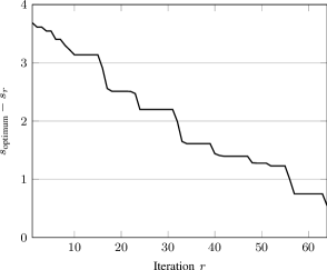
Figure 2: Convergence of the proposed SL-RGS to the unrestricted GS algorithm with $M^{\prime}=2$, $N=4$, $N_{r}=64$ and $K=8$.

This indicates that the proposed SL-RGS algorithm leads to a close to optimal result in terms of $s_{r}$, i.e. $s_{r}\rightarrow s_{\rm optimum}$ provided that the range $2\beta$ is sufficiently large. This discussion aims to give insight on how the proposed SL-RGS algorithm can obtain satisfactory results provided the range $2\beta$ is chosen sufficiently large.

V-B Computational Complexity

V-B1 GEVD vs SL-FS

In the GEVD algorithm, the operations that contribute the most to the computational complexity lie in the eigenvalue decomposition and matrix multiplications. While in the SL-FS algorithms, the operation of trace in each iteration consumes most of the calculations. The computational complexities of the illustrated design algorithms are shown in Table II, where $\mathcal{O}(\cdot)$ represents the big O notation.

TABLE II: Computational complexity of the illustrated matrix design algorithms

The solid lines in Fig. 3 represent the computational complexity of the three matrix design algorithms studied. It is noticed that the SL-RGS algorithm consumes roughly the same complexity as the GEVD and the SL-BFS algorithm has the highest complexity. The complexity of the simplified SL-BFS and SL-RGS are shown as the dashed lines in Fig. 3. Compared to the standard SL-BFS and SL-RGS algorithms, the simplified SL-FS recursions can provide savings of up to 87.5% of the computational costs.

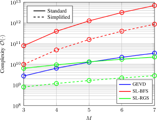
Figure 3: Computational complexity of analyzed matrix design algorithms as a function of initial sampling rate, which is $M$ times the Nyquist rate, where $N=4,N_{r}=64,M^{\prime}=2,\beta=5$ and $K=8$

V-B2 Uniform vs Dynamic Oversampling

The comparison of the computational complexity of different oversampling techniques using the MSE based design is examined here. We remark that the window technique is considered for both uniform and dynamic oversampling schemes. In systems with uniform oversampling, all received samples are used for signal processing, which means that there is no need for the pattern design and dimension reduction. The corresponding sliding window based LRA-MMSE detector is a modified version of (35), which is described by

$$\mathbf{W}_{\text{LRA-MMSE}}^{\text{uni}}=\mathbf{C}_{\mathbf{y}_{\mathcal{Q}_{\text{win}}}}^{-1}\mathbf{C}_{\mathbf{y}_{\mathcal{Q}_{\text{win}}}\mathbf{x}_{\text{win}}}.$$ (50)

Table III shows the computational complexity of different oversampling techniques for obtaining the detected symbols in each window with the known pattern design. Assuming that the whole transmission block including the operation of pattern design, which is obtained only once at the beginning of each transmission, and dimension reduction, which is applied in each window, in systems with dynamic oversampling the total complexity comparison between uniform and dynamic oversampling techniques are shown in Fig. 4. It can be noticed that both the standard and simplified SL-RGS based dynamic oversampling techniques require the lowest computational cost among the studied oversampling techniques. We remark that the complexity reduction for dynamic oversampling comes from the fact that a lower processing rate $M^{\prime}=2$ is used regardless of the sampling rate $M$, while the black curve from uniform sampling increases the processing rate together with the sampling rate $M^{\prime}=M$. Compared to the standard algorithm, the simplified SL-BFS and SL-RGS have saved up to 87.33% and 54.16% in terms of computational costs, respectively. When compared with uniform oversampling, dynamic oversampling with the GEVD and the simplified SL-RGS techniques can save up to 54.99% and 97.13% in terms of computational costs, respectively.

TABLE III: Computational complexity for obtaining the detected symbols in each window

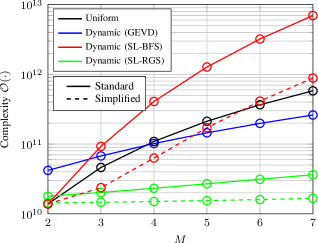
Figure 4: Detection complexity of uniform ($M=M^{\prime}$) and dynamic oversampling in one transmission block (containing 100 symbols) as a function of initial sampling rate, which is $M$ times the Nyquist rate, where $l=4,N_{r}=64,N_{t}=4,M^{\prime}=2,\beta=5$ and $K=8$.

V-C The choice of $K$ and $\beta$

The SL-FS algorithm has the large dimensional matrix $\mathbf{\Delta}_{B}$ partitioned into $K$ low dimensional submatrices $\mathbf{\Delta}_{B_{k}}$ for computational purposes. In this subsection, we discuss further the impact of $K$ on the system performance. Specifically, $K$ is chosen as the divisor of $M^{\prime}NN_{r}$, namely $\mod(M^{\prime}NN_{r},K)=0$. Fig. 5(a) shows the sum rate performance and the detection complexity by using the simplified SL-RGS dynamic oversampling technique as a function of $K$, where both decrease with the increase of $K$. These results indicate that the parameter $K$ should be chosen properly in order to obtain satisfactory sum rate performance and low detection complexity. Moreover, Fig. 5(b) shows the sum rate and the detection complexity as a function of $\beta$. In the SL-RGS algorithm, the pre-defined parameter $\beta$ controls the search range in each row. From the results, it is seen that beyond $\beta=5$ there are diminishing returns on the sum rate performance.

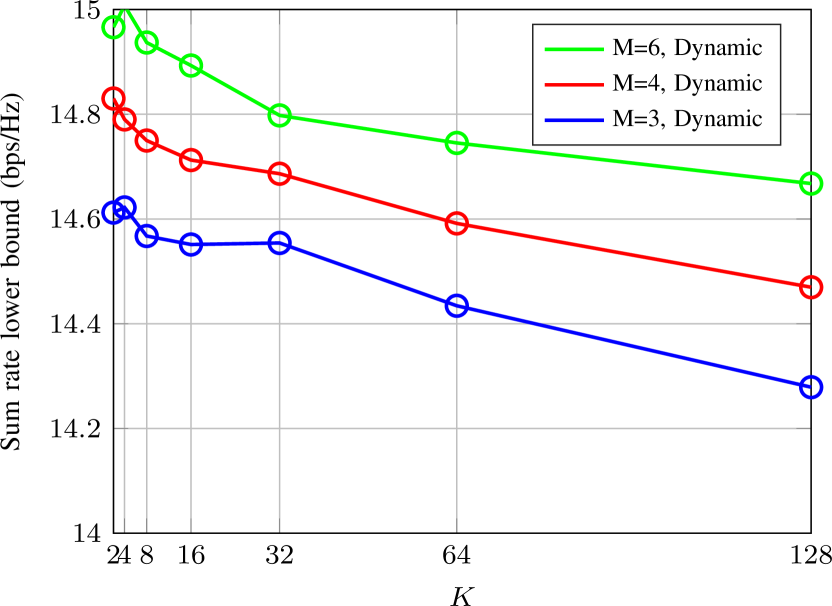
(a) $\beta=5$

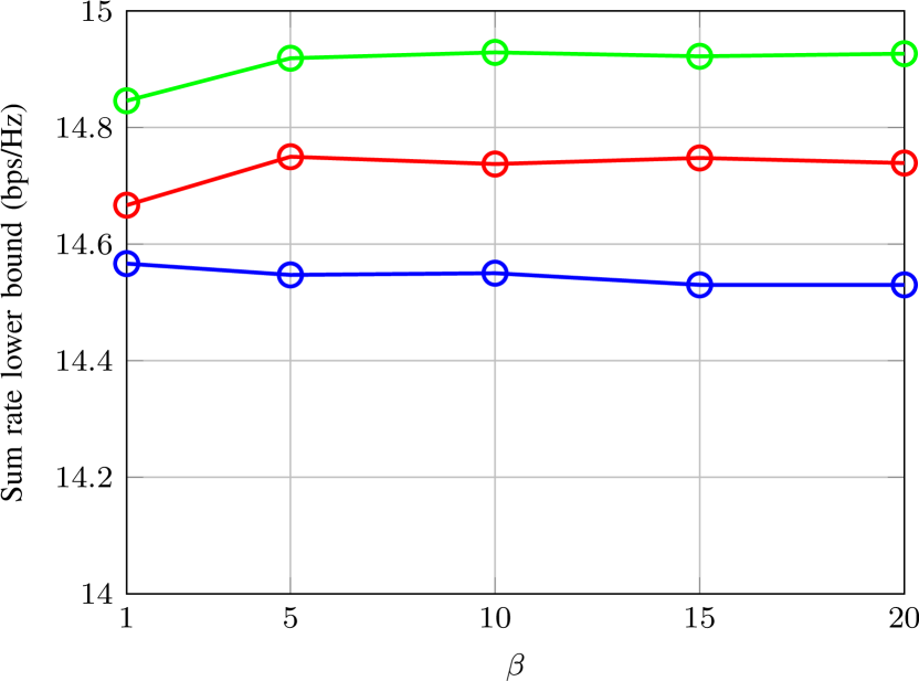
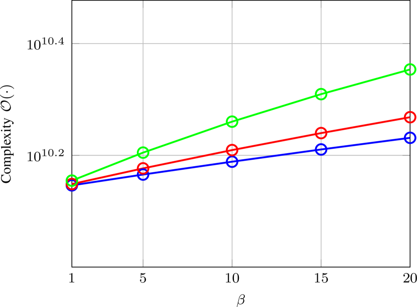
(b) $K=8$

Figure 5: The sum rate performance ($N=4$) and detection complexity in one transmission block (containing 100 symbols) as a function of $K$ and $\beta$ with $l=4,N_{r}=64,M^{\prime}=2$.

V-D Power Consumption

Here, we investigate the receiver power consumption of systems with uniform and dynamic oversampling versus the number of bits used by the ADCs. Fig. 6 shows the simplified power consumption $P$ at the receiver as a function of the quantization bits $b$, where only the power consumption of different components among different systems is considered. The simplified power consumption is calculated as

$$P=2N_{r}(cP_{\text{AGC}}+P_{\text{ADC}}),$$ (51)

where $P_{\text{AGC}}$ denotes the power consumption of AGC. $c$ is chosen as 0 for 1-bit system and 1 for systems with more-bits. The $P_{\text{ADC}}$ is given by

$$P_{\text{ADC}}=\text{FOM}_{w}\times Mf_{\text{Nyquist}}\times 2^{b},\quad b=1,2,\cdots$$ (52)

where $f_{\text{Nyquist}}$ is the Nyquist-sampling rate. Numerical parameters are based on [42], where $P_{\text{AGC}}=2$mW, $\text{FOM}_{w}$ is 200 fJ/conversion-step at 50 MHz bandwidth and $f_{\text{Nyquist}}$ is 100 MHz. Fig. 6 shows the simplified power consumption as a function of the sampling rate, where the 1-bit system consumes the least power.

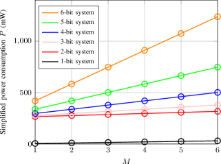
Figure 6: Simplified power consumption at the receiver with $N_{r}=64$.

VI Numerical Results

In this section, the uplink of a large-scale MIMO system [43, wence] with $N_{r}=64$ and $N_{t}=4$ users is considered. The $m(t)$ and $p(t)$ are normalized root-raised-cosine (RRC) filters with a roll-off factor of 0.8 and the time delay $n^{d}_{n_{t}}$ of each terminal is uniformly distributed between $-T$ and $T$. The channel is assumed to experience Rayleigh block fading. The simulation results presented here are obtained by averaging over 1000 independent realizations of the channel matrix $\mathbf{H^{\prime}}$, noise and symbol vectors. The SNR is defined as $10\log(\frac{N_{t}}{\sigma_{n}^{2}})$. In systems with dynamic oversampling [44], the performance of different initial sampling rates are compared under the condition that the signal processing rates $M^{\prime}$ are equal to 2. In the SL-BFS and SL-RGS algorithms $\beta=5$ and $K=8$.

VI-A Design based on the sum rate criterion

We first consider the system design based on the sum rate criterion, where each transmission block contains 4 symbols and Gaussian signaling is assumed. Fig. 7(a) shows the sum rate performance of systems with uniform and GEVD based dynamic oversampling, where the latter outperforms the former. Fig. 7(b) compares the performance of SL-RGS based dynamic oversampling technique with standard and simplified version. As depicted in Fig. 7(b), the performance of the simplified and the standard SL-RGS algorithms are comparable, and dynamic oversampling with both versions outperforms uniform oversampling. In terms of complexity, the proposed simplified SL-FS algorithms have a much lower computational cost than the standard SL-FS algorithms, while their performance are comparable. Fig. 7(b) also compares the performance of the simplified SL-FS algorithms, where both SL-BFS and SL-RGS achieve similar sum rates . Figs. 7(a) and 7(b) show that among the compared dimension reduction algorithms the GEVD outperforms the SL-FS algorithms, since more information is exploited and the samples are combined, but the simplified SL-FS algorithms require lower computational costs. The green lines (Dynamic, $M=6$, $M^{\prime}=2$) in the figures indicate that a sum-rate performance gain of up to 10% over that of uniform oversampling with $M=2$ can be achieved.

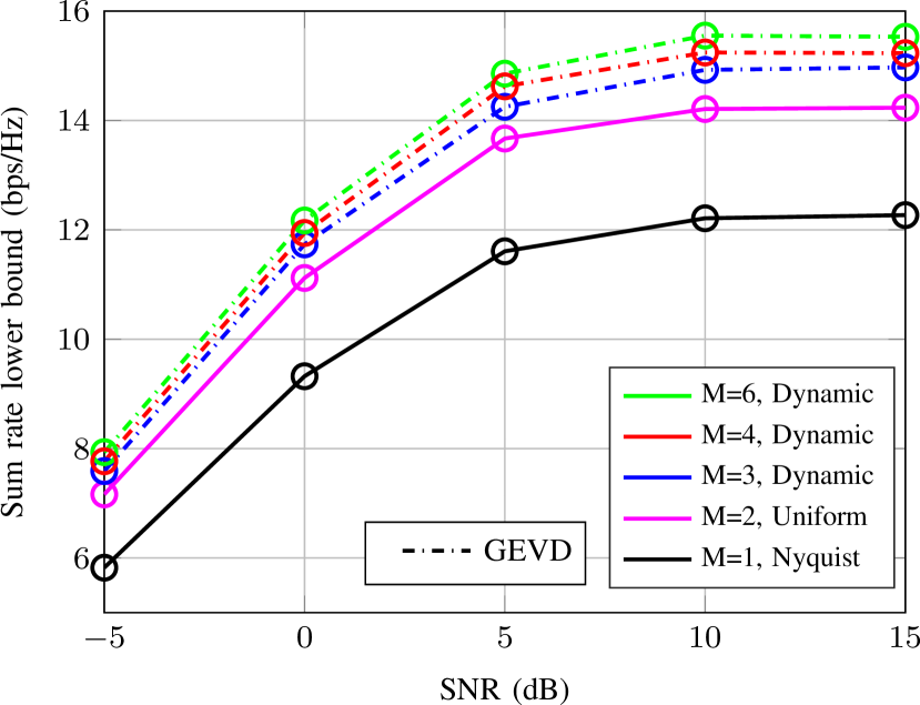
(a) GEVD

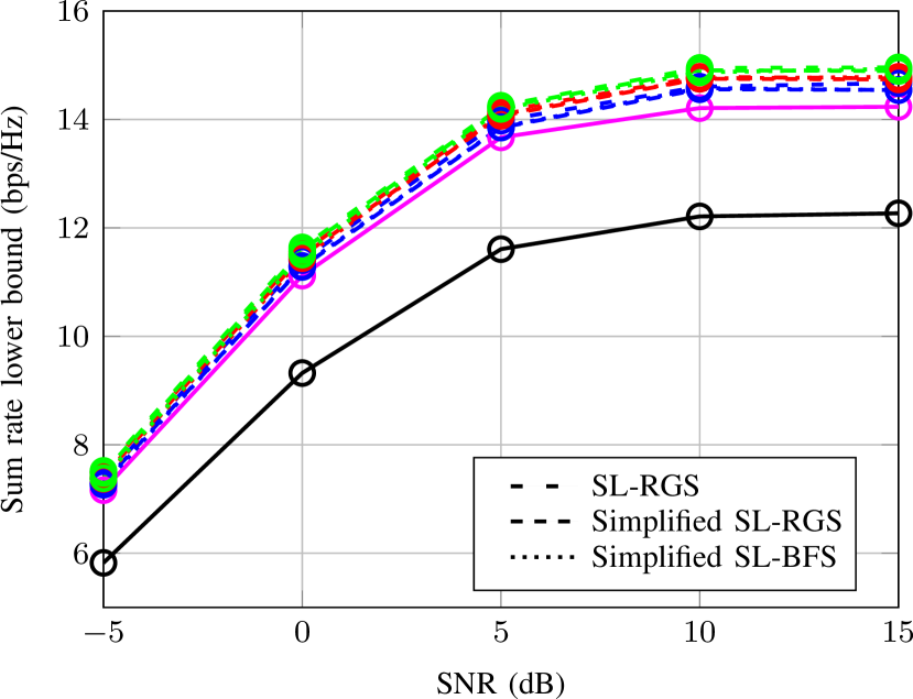
(b) SL-FS

Figure 7: Comparison among Nyquist sampling, uniform oversampling and GEVD and SL-FS based dynamic oversampling with $M^{\prime}=2$.

VI-B Design based on the MSE criterion

In this subsection, we examine the proposed dynamic oversampling techniques in terms of the normalized MSE and SER. The modulation scheme is quadrature phase-shift keying (QPSK). Each transmission block contains 100 symbols. The window length $l$ is chosen as 4 Nyquist-sampled symbols.

Figs. 8(a) and 8(b) show the normalized MSE performance as a function of SNR with GEVD based dynamic oversampling, respectively. The results show that dynamic oversampling outperforms uniform oversampling with $M=2$ while making the signal detection. In terms of complexity, Fig. 4 shows the GEVD based dynamic oversampling has higher complexity than uniform oversampling with $M=2$. This reveals the complexity disadvantages of the GEVD based dynamic oversampling technique.

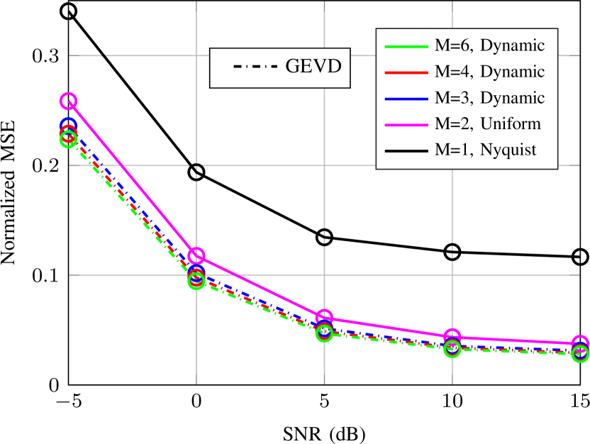
(a) GEVD

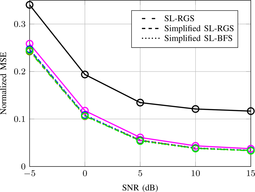
(b) SL-FS

Figure 8: Comparison among Nyquist sampling, uniform oversampling and GEVD and SL-FS based dynamic oversampling with $M^{\prime}=2$.

Furthermore, Figs. 9 and 10 show the SER performance of the GEVD and SL-FS based dynamic oversampling technique, respectively. It can be seen that the SL-RGS based dynamic oversampling outperforms uniform oversampling with $M=2$ without increasing the computational cost. This reveals the performance advantages of the proposed SL-RGS based dynamic oversampling techniques. Moreover, in Fig. 10 the SER performance of the simplified SL-BFS and the simplified SL-RGS algorithms is also compared. The simplified SL-BFS and the simplified SL-RGS with $M^{\prime}=2$ have similar performance, whereas they significantly outperform uniform oversampling. Figs. 9 and 10 have also compared the SER performance of the proposed LRA-MMSE detector and dynamic oversampling scheme with other existing 1-bit detectors with sampling at the Nyquist rate [13] and uniform oversampling [45], where the former achieves the best performance.

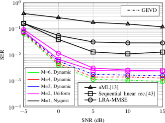
Figure 9: Comparison among Nyquist sampling, uniform oversampling and GEVD based dynamic oversampling with $M^{\prime}=2$.

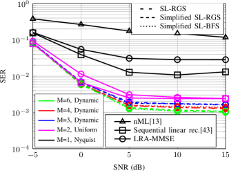
Figure 10: Comparison among Nyquist sampling, uniform oversampling and SL-FS based dynamic oversampling technique with $M^{\prime}=2$.

In order to further investigate the practical benefits of the proposed dynamic oversampling technique, we have compared the analyzed systems using $N_{t}=12$, $N_{r}=32$ and Low-Density Parity-Check (LDPC) codes with block length $n=512$ and rate $R=1/2$ [46] using an iterative detection and decoding scheme [14]. Other iterative detection and decoding schemes [47, 48, 49, 50, 51, 52, 53, 54] are also possible. Fig. 11 shows the bit error rate (BER) performance of the coded systems, where Eb/No is defined as $10\log(\frac{N_{t}R}{\sigma_{n}^{2}})$. The results show that the proposed dynamic oversampling outperforms the existing uniform oversampling and Nyquist-rate techniques.

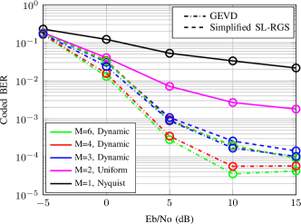
Figure 11: Comparison between GEVD and simplified SL-RGS based dynamic oversampling with $M^{\prime}=2$.

VII Conclusions

This work has proposed dynamic oversampling techniques for large-scale multiple-antenna systems with 1-bit quantization at the receiver. We have developed designs based on the sum rate and the MSE criteria. Dimension reduction algorithms have also been devised based the GEVD and sparse binary matrices in order to perform dynamic oversampling. Furthermore, the proposed techniques have been analyzed in terms of convergence, computational complexity and power consumption at the receiver. Simulation results have shown that the proposed dynamic oversampling can outperform uniform oversampling in terms of sum rate, MSE or SER performance but with much lower computational costs.

References

- [1] E. G. Larsson, O. Edfors, F. Tufvesson, and T. L. Marzetta, “Massive MIMO for next generation wireless systems,” IEEE Commun. Mag., vol. 52, no. 2, pp. 186–195, Feb. 2014.
- [2] H. Q. Ngo, E. G. Larsson, and T. L. Marzetta, “Energy and Spectral Efficiency of Very Large Multiuser MIMO Systems,” IEEE Trans. Commun., vol. 61, no. 4, pp. 1436–1449, Apr. 2013.
- [3] F. Boccardi, R. W. Heath, A. Lozano, T. L. Marzetta, and P. Popovski, “Five disruptive technology directions for 5G,” IEEE Commun. Mag., vol. 52, no. 2, pp. 74–80, Feb. 2014.
- [4] J. G. Andrews, S. Buzzi, W. Choi, S. V. Hanly, A. Lozano, A. C. K. Soong, and J. C. Zhang, “What Will 5G be?” IEEE J. Sel. Areas Commun., vol. 32, no. 6, pp. 1065–1082, Jun. 2014.
- [5] R. H. Walden, “Analog-to-digital converter survey and analysis,” IEEE J. Sel. Areas Commun., vol. 17, no. 4, pp. 539–550, Apr. 1999.
- [6] J. Singh, S. Ponnuru, and U. Madhow, “Multi-Gigabit communication: the ADC bottleneck1,” in IEEE International Conference on Ultra-Wideband, Sep. 2009, pp. 22–27.
- [7] S. Jacobsson, G. Durisi, M. Coldrey, U. Gustavsson, and C. Studer, “Throughput analysis of massive MIMO uplink with low-resolution ADCs,” IEEE Trans. Wireless Commun., vol. 16, no. 6, pp. 4038–4051, Jun. 2017.
- [8] J. Mo and R. W. Heath, “Capacity Analysis of One-Bit Quantized MIMO Systems With Transmitter Channel State Information,” IEEE Trans. Signal Process., vol. 63, no. 20, pp. 5498–5512, Oct. 2015.
- [9] A. Mezghani and J. A. Nossek, “Capacity lower bound of MIMO channels with output quantization and correlated noise,” in Proc. IEEE Int. Symp. Inform. Theory (ISIT), Boston, USA, Jul. 2012.
- [10] Y. Li, C. Tao, G. Seco-Granados, A. Mezghani, A. L. Swindlehurst, and L. Liu, “Channel estimation and performance analysis of one-bit massive MIMO systems,” IEEE Trans. Signal Process., vol. 65, no. 15, pp. 4075–4089, Aug. 2017.
- [11] C. Stöckle, J. Munir, A. Mezghani, and J. A. Nossek, “Channel estimation in massive MIMO systems using 1-bit quantization,” in IEEE 17th Int. Workshop on Signal Process. Advances in Wireless Comm. (SPAWC), Jul. 2016.
- [12] Z. Shao, R. C. de Lamare, and L. T. N. Landau, “Adaptive Channel Estimation and Interference Mitigation for Large-Scale MIMO Systems with 1-Bit ADCs,” in 15th International Symposium on Wireless Communication Systems (ISWCS), Aug. 2018, pp. 1–5.
- [13] J. Choi, J. Mo, and R. W. Heath, “Near Maximum-Likelihood Detector and Channel Estimator for Uplink Multiuser Massive MIMO Systems With One-Bit ADCs,” IEEE Trans. Commun., vol. 64, no. 5, pp. 2005–2018, May 2016.
- [14] Z. Shao, R. C. Lamare, and L. T. N. Landau, “Iterative detection and decoding for large-scale multiple-antenna systems with 1-bit ADCs,” IEEE Wireless Commun. Lett., vol. 7, no. 3, pp. 476–479, Jun. 2018.
- [15] Y. Jeon, N. Lee, S. Hong, and R. W. Heath, “One-bit sphere decoding for uplink massive MIMO systems with one-bit ADCs,” IEEE Trans. Wireless Commun., vol. 17, no. 7, pp. 4509–4521, Jul. 2018.
- [16] Y. Jeon, H. Do, S. Hong, and N. Lee, “Soft-Output Detection Methods for Sparse Millimeter-Wave MIMO Systems With Low-Precision ADCs,” IEEE Trans. Commun., vol. 67, no. 4, pp. 2822–2836, 2019.
- [17] S. Hong, S. Kim, and N. Lee, “A Weighted Minimum Distance Decoding for Uplink Multiuser MIMO Systems With Low-Resolution ADCs,” IEEE Trans. Commun., vol. 66, no. 5, pp. 1912–1924, 2018.
- [18] A. K. Saxena, I. Fijalkow, and A. L. Swindlehurst, “Analysis of one-bit quantized precoding for the multiuser massive MIMO downlink,” IEEE Trans. Signal Process., vol. 65, no. 17, pp. 4624–4634, Sep. 2017.
- [19] L. T. N. Landau and R. C. de Lamare, “Branch-and-bound precoding for multiuser MIMO systems with 1-bit quantization,” IEEE Wireless Commun. Lett., vol. 6, no. 6, pp. 770–773, Dec. 2017.
- [20] H. Jedda, A. Mezghani, J. A. Nossek, and A. L. Swindlehurst, “Massive MIMO downlink 1-bit precoding with linear programming for PSK signaling,” in IEEE 18th International Workshop on Signal Processing Advances in Wireless Communications (SPAWC), Jul. 2017.
- [21] G. Park and S. Hong, “Construction of 1-Bit Transmit-Signal Vectors for Downlink MU-MISO Systems With PSK Signaling,” IEEE Trans. Veh. Commun., vol. 68, no. 8, pp. 8270–8274, 2019.
- [22] C. Studer and G. Durisi, “Quantized massive MU-MIMO-OFDM uplink,” IEEE Trans. Commun., vol. 64, no. 6, pp. 2387–2399, Jun. 2016.
- [23] C. Mollén, J. Choi, E. G. Larsson, and R. W. Heath, “Uplink performance of wideband massive MIMO with one-bit ADCs,” IEEE Trans. Wireless Commun., vol. 16, no. 1, pp. 87–100, Jan. 2017.
- [24] J. Zhang, L. Dai, X. Li, Y. Liu, and L. Hanzo, “On low-resolution ADCs in practical 5G millimeter-wave massive MIMO systems,” IEEE Commun. Mag., vol. 56, no. 7, pp. 205–211, Jul. 2018.
- [25] E. N. Gilbert, “Increased information rate by oversampling,” IEEE Trans. Inf. Theory, vol. 39, no. 6, pp. 1973–1976, Nov. 1993.
- [26] T. Koch and A. Lapidoth, “Increased capacity per unit-cost by oversampling,” in 2010 IEEE 26-th Convention of Electrical and Electronics Engineers in Israel, Nov. 2010, pp. 684–688.
- [27] T. Halsig, L. Landau, and G. Fettweis, “Information Rates for Faster-Than-Nyquist Signaling with 1-Bit Quantization and Oversampling at the Receiver,” in IEEE 79th Vehicular Technology Conference (VTC Spring), May 2014.
- [28] A. B. Üçüncü and A. O. Yılmaz, “Oversampling in One-Bit Quantized Massive MIMO Systems and Performance Analysis,” IEEE Trans. Wireless Commun., vol. 17, no. 12, pp. 7952–7964, Dec. 2018.
- [29] Z. Shao, L. T. N. Landau, and R. C. de Lamare, “Channel Estimation Using 1-Bit Quantization and Oversampling for Large-scale Multiple-antenna Systems,” in Proc. IEEE Int. Conf. Acoust., Speech, Signal Process., May 2019, pp. 4669–4673.
- [30] Z. Shao, L. T. N. Landau, and R. C. De Lamare, “Channel Estimation for Large-Scale Multiple-Antenna Systems Using 1-Bit ADCs and Oversampling,” IEEE Access, vol. 8, pp. 85 243–85 256, 2020.
- [31] Z. Shao, L. T. N. Landau, and R. C. de Lamare, “Sliding Window Based Linear Signal Detection Using 1-Bit Quantization and Oversampling for Large-Scale Multiple-Antenna Systems,” in IEEE Statistical Signal Processing Workshop (SSP), Jun. 2018, pp. 183–187.
- [32] ——, “Dynamic oversampling in 1-bit quantized asynchronous large-scale multiple-antenna systems for sustainable IoT networks,” in Proc. IEEE Int. Conf. Acoust., Speech, Signal Process., May 2020.
- [33] J. J. Bussgang, “Crosscorrelation functions of amplitude-distorted Gaussian signals,” Res. Lab. Elec., MIT, vol. Tech. Rep. 216, Mar. 1952.
- [34] G. Jacovitti and A. Neri, “Estimation of the autocorrelation function of complex Gaussian stationary processes by amplitude clipped signals,” IEEE Trans. Inf. Theory, vol. 40, no. 1, pp. 239–245, Jan. 1994.
- [35] R. C. de Lamare and R. Sampaio-Neto, “Adaptive Reduced-Rank Processing Based on Joint and Iterative Interpolation, Decimation, and Filtering,” IEEE Trans. Signal Process., vol. 57, no. 7, pp. 2503–2514, Jul. 2009.
- [36] S. Boyd and L. Vandenberghe, Convex optimization. Cambridge university press, 2004.
- [37] H. Wang, S. Yan, D. Xu, X. Tang, and T. Huang, “Trace Ratio vs. Ratio Trace for Dimensionality Reduction,” in IEEE Conference on Computer Vision and Pattern Recognition, Jun. 2007.
- [38] Y. Jia, F. Nie, and C. Zhang, “Trace Ratio Problem Revisited,” IEEE Trans. Neural Netw., vol. 20, no. 4, pp. 729–735, Apr. 2009.
- [39] B. Ghojogh, F. Karray, and M. Crowley, “Eigenvalue and Generalized Eigenvalue Problems: Tutorial,” 2019.
- [40] P. Devijver and J. Kittler, Pattern Recognition: A Statistical Approach. Prentice-Hall, 1982.
- [41] J. Kittler, “Feature set search algorithms,” Pattern recognition and signal processing, 1978.
- [42] Y. Xiong, Z. Zhang, N. Wei, B. Li, and Y. Chen, “Performance analysis of uplink massive MIMO systems with variable-resolution ADCs using MMSE and MRC detection,” Transactions on Emerging Telecommunications Technologies, vol. 30, no. 5, p. 3549, 2019.
- [43] R. C. de Lamare, “Massive mimo systems: Signal processing challenges and future trends,” URSI Radio Science Bulletin, vol. 2013, no. 347, pp. 8–20, 2013.
- [44] Z. Shao, L. T. N. Landau, and R. C. de Lamare, “Dynamic oversampling for 1-bit adcs in large-scale multiple-antenna systems,” IEEE Transactions on Communications, pp. 1–1, 2021.
- [45] A. B. Üçüncü and A. O. Yılmaz, “Sequential Linear Detection in One-Bit Quantized Uplink Massive MIMO with Oversampling,” in 2018 IEEE 88th Vehicular Technology Conference (VTC-Fall), 2018, pp. 1–5.
- [46] C. T. Healy and R. C. de Lamare, “Design of ldpc codes based on multipath emd strategies for progressive edge growth,” IEEE Transactions on Communications, vol. 64, no. 8, pp. 3208–3219, 2016.
- [47] R. C. De Lamare and R. Sampaio-Neto, “Minimum mean-squared error iterative successive parallel arbitrated decision feedback detectors for ds-cdma systems,” IEEE Transactions on Communications, vol. 56, no. 5, pp. 778–789, 2008.
- [48] P. Li, R. C. de Lamare, and R. Fa, “Multiple feedback successive interference cancellation detection for multiuser mimo systems,” IEEE Transactions on Wireless Communications, vol. 10, no. 8, pp. 2434–2439, 2011.
- [49] P. Li and R. C. De Lamare, “Adaptive decision-feedback detection with constellation constraints for mimo systems,” IEEE Transactions on Vehicular Technology, vol. 61, no. 2, pp. 853–859, 2012.
- [50] R. C. de Lamare, “Adaptive and iterative multi-branch mmse decision feedback detection algorithms for multi-antenna systems,” IEEE Transactions on Wireless Communications, vol. 12, no. 10, pp. 5294–5308, 2013.
- [51] P. Li and R. C. de Lamare, “Distributed iterative detection with reduced message passing for networked mimo cellular systems,” IEEE Transactions on Vehicular Technology, vol. 63, no. 6, pp. 2947–2954, 2014.
- [52] A. G. D. Uchoa, C. T. Healy, and R. C. de Lamare, “Iterative detection and decoding algorithms for mimo systems in block-fading channels using ldpc codes,” IEEE Transactions on Vehicular Technology, vol. 65, no. 4, pp. 2735–2741, 2016.
- [53] Y. Cai, R. C. de Lamare, B. Champagne, B. Qin, and M. Zhao, “Adaptive reduced-rank receive processing based on minimum symbol-error-rate criterion for large-scale multiple-antenna systems,” IEEE Transactions on Communications, vol. 63, no. 11, pp. 4185–4201, 2015.
- [54] R. B. Di Renna and R. C. de Lamare, “Iterative list detection and decoding for massive machine-type communications,” IEEE Transactions on Communications, vol. 68, no. 10, pp. 6276–6288, 2020.