Flexible Model Aggregation for Quantile Regression

Abstract

Quantile regression is a fundamental problem in statistical learning motivated by a need to quantify uncertainty in predictions, or to model a diverse population without being overly reductive. For instance, epidemiological forecasts, cost estimates, and revenue predictions all benefit from being able to quantify the range of possible values accurately. As such, many models have been developed for this problem over many years of research in statistics, machine learning, and related fields. Rather than proposing yet another (new) algorithm for quantile regression we adopt a meta viewpoint: we investigate methods for aggregating any number of conditional quantile models, in order to improve accuracy and robustness. We consider weighted ensembles where weights may vary over not only individual models, but also over quantile levels, and feature values. All of the models we consider in this paper can be fit using modern deep learning toolkits, and hence are widely accessible (from an implementation point of view) and scalable. To improve the accuracy of the predicted quantiles (or equivalently, prediction intervals), we develop tools for ensuring that quantiles remain monotonically ordered, and apply conformal calibration methods. These can be used without any modification of the original library of base models. We also review some basic theory surrounding quantile aggregation and related scoring rules, and contribute a few new results to this literature (for example, the fact that post sorting or post isotonic regression can only improve the weighted interval score). Finally, we provide an extensive suite of empirical comparisons across 34 data sets from two different benchmark repositories.

Keywords: quantile regression, model aggregation, neural networks

1 Introduction

Consider the problem of assessing the height of a child. Common practice is to consult a growth chart, such as the ones provided by the CDC (Kuczmarski, 2000) and to review the distribution of heights, as relevant to the age and sex of the child. In doing so, the medical practitioner performs quantile regression, conditioning their estimates on covariates (age, sex) to obtain a conditional height distribution. While it would be possible to employ more standard regression methods for this problem, which would deliver an estimate of the mean height as a function of the covariates, quantile regression provides something more: it gives us a sense of what to expect in the spread of the response variable (height) as a function of the covariates.

The development of tools for conditional quantile estimation has a rich history in both econometrics and statistics. These tools are widely-used for quantifying uncertainty, and also for characterizing heterogeneous outcomes across diverse populations. As this is an important problem, many methods to arrive at quantile estimates abound. It stands to reason that a combination of different techniques can improve on the accuracy offered by individual base estimates. Precisely in this vein, the current paper considers the problem of model aggregation, i.e., the task of combining any number of quantile regression models into a unified estimator.

To fix notation, let $Y\in\mathbb{R}$ be a response variable of interest, and $X\in\mathcal{X}$ be an input feature vector used to predict $Y$. A generic way to approach uncertainty quantification is to estimate the conditional distribution of $Y|X=x$. However, this can be a formidable challenge, especially in high dimensions ($\mathcal{X}=\mathbb{R}^{d}$, where $d$ is large). A simpler alternative is to estimate conditional quantiles of $Y|X=x$ across a discrete set of quantile levels $\mathcal{T}\subseteq[0,1]$, that is, to estimate $g^{*}(x;\tau)=F^{-1}_{Y|X=x}(\tau)$ for $\tau\in\mathcal{T}$. Here, for a random variable $Z$ with a cumulative distribution function (CDF) $F_{Z}$, we denote its level $\tau$ quantile by

$$F^{-1}_{Z}(\tau)=\inf\{z:F_{Z}(z)\geq\tau\}.$$

For example, we might choose $\mathcal{T}=\{0.01,0.02,\ldots,0.99\}$ to finely characterize the spread of $Y|X=x$.

The aggregation problem can be motivated as follows. Suppose we have a number of conditional quantile estimates, for instance, through a set of different quantile regression methods, or various teams submitting their estimates to a consensus board or as entries in a prediction competition. In all of these cases, we need an automated strategy to determine which estimate(s) of which quantile level(s) should be combined into a consensus model.

More formally, suppose we have a collection $\{\hat{g}_{j}\}_{j=1}^{p}$ of conditional quantile models, parametrized by a set of common quantile levels $\mathcal{T}$. Each model $\hat{g}_{j}$, which we refer to as a base model, provides an estimate of the true conditional quantile function $g^{*}$. It is convenient to view $g^{*}$, and each $\hat{g}_{j}$, as functions from $\mathcal{X}$ to $\mathbb{R}^{m}$, so that $g^{*}(x)$ outputs a vector of dimension $m=|\mathcal{T}|$, the number of quantile levels. We denote the components of this vector by $g^{*}(x;\tau)$ for $\tau\in\mathcal{T}$, and similarly for each $\hat{g}_{j}(x)$. Given $p\times m$ estimates of $m$ quantile levels by $p$ base models, each one a function of $x\in\mathcal{X}$, we will study ensemble estimates, of the generic form:

$$\hat{g}=H(\hat{g}_{1},\ldots,\hat{g}_{p})\,:\,\mathcal{X}\to\mathbb{R}^{m}.$$

In this paper, we focus on linear aggregation procedures $H$, though we allow the aggregation weights in these linear combinations to be themselves functions of input feature values $x$, as in:

$$\hat{g}_{w}(x)=\sum_{j=1}^{p}w_{j}(x)\cdot\hat{g}_{j}(x),\quad x\in\mathcal{X}.$$ (1)

This form may seem overly restrictive. That said, each term $\hat{g}_{j}$ on its own can be quite powerful. Moreover, as we show later, a sufficiently flexible parametrization for the weight functions can provide all the modeling power that we need. In particular, we will consider various aggregation strategies in which each weight $w_{j}(x)$ is a scalar, vector, or matrix. The product “$\cdot$” between $w_{j}(x)$ and $\hat{g}_{j}(x)$ in (1) is to be interpreted accordingly (more below).

Our main purpose in what follows is to provide a guided tour of how one might go about fitting quantile aggregation models of the form (1), of varying degrees of flexibility, and to walk through some of the major practical considerations that accompany fitting and evaluating such models. The aggregation strategies that we consider can be laid out over the following two dimensions.

1. Coarse versus medium versus fine: this dimension determines the resolution for the parametrization of the weights in (1).

   • A coarse aggregator uses one weight $w_{j}$ per base model $\hat{g}_{j}$, and we accordingly interpret “$\cdot$” in (1) as a scalar-vector product.

   • A medium aggregator uses one weight $w^{\tau}_{j}$ per base model $\hat{g}_{j}$ and quantile level $\tau$, and we interpret “$\cdot$” in (1) as a Hadamard (elementwise) product between vectors. This allows us to place a higher amount of weight for a given model in the tails versus the center the distribution.

   • A fine aggregator uses one weight $w^{\tau,\nu}_{j}$ per base model $\hat{g}_{j}$, output quantile level $\tau$ (for the output quantile), and input quantile level $\nu$ (from a base model), and we interpret “$\cdot$” in (1) as a matrix-vector product. This allows us to use all of the quantiles from all base models in order to form an estimate at a single quantile level for the aggregate model (e.g., the aggregate median is informed by all quantiles from all base models, not just their medians).

2. Global versus local: this dimension determines whether or not the weights in (1) depend on $x$. A global aggregator uses constant weights, $w_{j}(x)=w_{j}$ for all $x\in\mathcal{X}$, whereas a local aggregator allows these to vary locally (and typically smoothly) in $x$.

Apart from model frameworks, the considerations we give the most attention to revolve around ensuring quantile noncrossing: $\hat{g}(x;\tau)\leq\hat{g}(x;\tau^{\prime})$ for any $x$ and $\tau<\tau^{\prime}$; and calibration: $\hat{g}(x;\tau^{\prime})-\hat{g}(x;\tau)$ contains the response variable with probability $\approx\tau^{\prime}-\tau$, at least in some average sense over $x\in\mathcal{X}$. Finally, we approach all of this work through the lens of the deep learning, designing methodology to be compatible with standard deep learning optimization toolkits so as to leverage their convenience of implementation and scalability.

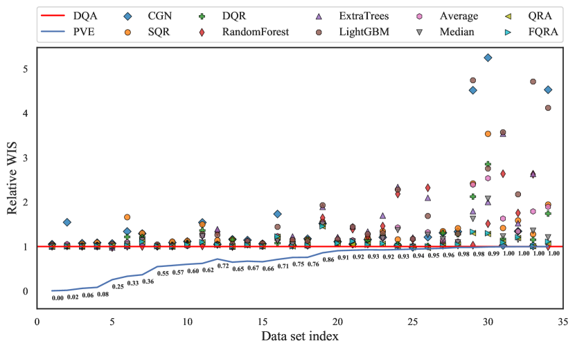
Figure 1: Weighted interval score (WIS), averaged over out-of-sample predictions, for deep quantile aggregation (DQA) and various quantile regression methods. DQA is the most flexible aggregation model of the form (1) that we consider in this paper. The comparison is made over 34 data sets, ordered along the x-axis by proportion of variance explained (PVE), as in (2). The y-axis displays the WIS of each method relative to DQA, so that 1 indicates equal performance to DQA, and a number greater than 1 indicates worse performance than DQA. We can see that DQA performs very well overall, especially for larger PVE values (problems with higher signal-to-noise ratios).

Before delving into any further details, we present some of our main empirical results in Figure 1. Here and henceforth we use the term deep quantile aggregation (DQA) to refer to the aggregation model in our framework with the greatest degree of flexibility, a local fine aggregator where the local weights are fit using a deep neural network, and we use an adaptive noncrossing penalty, along with gradient propogation of the min-max sweep isotonization operator, to ensure quantile noncrossing (Section 4 provides more details). The figure compares DQA and various other quantile regression methods across 34 data sets (Section 6 gives more details). The error metric we use is weighted interval score (WIS), averaged over out-of-sample predictions (lower WIS is better; more details are given in the next section).

Shown on the y-axis is the relative WIS of each quantile regression method to DQA, where 1 indicates equal WIS performance to DQA, and a number greater than 1 indicates worse performance than DQA. Each point on the x-axis represents a data set, and we order them by increasing proportion of variance explained (PVE), measured with respect to DQA $\hat{g}$ (as a proxy for $g^{*}$) and test samples $(X^{*}_{i},Y^{*}_{i})$, $i=1,\ldots,m$ by:

$$\mathrm{PVE}(\hat{g})=1-\frac{\sum_{i=1}^{m}(Y^{*}_{i}-\hat{g}(X^{*}_{i};0.5))^{2}}{\sum_{i=1}^{m}(Y^{*}_{i}-\bar{Y}^{*})^{2}},$$ (2)

where $\hat{g}(x;0.5)$ denotes the estimate of the conditional median of $Y|X=x$ from DQA, and $\bar{Y}^{*}=\frac{1}{m}\sum_{i=1}^{m}Y^{*}_{i}$ is the sample mean of the test responses. The PVE curve itself is drawn in blue on the figure. The bottom four methods, according to the legend ordering, represent different aggregators, and the rest are individual base models (some are highly nonlinear and flexible themselves) that are fed into each aggregation procedure. As we can see, DQA performs very well across the board, and particularly for higher PVE values (which we can think of as problems that have higher signal-to-noise ratios, presenting a greater promise for the flexibility embodied by DQA), it can provide huge improvements on the base models and other aggregators. We should be clear that DQA is not uniformly better than all methods on all data sets—some points in the figure lie below 1. We provide an alternate visualization in in Appendix B.3 in which this is more clearly visible.

1.1 Related work

In this section, we briefly discuss previous work in quantile regression and model aggregation.

1.1.1 Quantile regression

Statistical modeling of quantiles dates back to Galton in the 1890s, however, many facts about quantiles were known long before (Hald, 1998). The modern view on conditional quantile models was pioneered by Koenker’s work on quantile regression in the 1970s (Koenker and Bassett, 1978); e.g., see Koenker and Hallock (2001); Koenker (2005) for nice overviews. This has remained a topic of great interest, with developments in areas such as kernel machines (Takeuchi et al., 2006), additive models (Koenker, 2011), high-dimensional regression (Belloni and Chernozhukov, 2011), and graphical models (Ali et al., 2016), just to name a few. Important developments in distribution-free calibration using quantile regression were given in Romano et al. (2019); Kivaranovic et al. (2020) (which we will return to later). The rise of deep learning has spurred on new progress in quantile regression with neural networks, e.g., Hatalis et al. (2017); Dabney et al. (2018); Xie and Wen (2019); Tagasovska and Lopez-Paz (2019); Benidis et al. (2022).

1.1.2 Model aggregation

Ensemble methods occupy a central place in machine learning (both in theory and in practice). Seminal work on this topic arose in the 1990s on Bayesian model averaging, bagging, boosting, and stacking; e.g., see Dietterich (2000) for a review. While the machine learning literature has mostly focused on ensembling point predictions, distributional ensembles have a long tradition in statistics, with a classic reference being Stone (1961). Combining distributional estimates is also of great interest in the forecasting community, see Raftery et al. (2005); Timmermann (2006); Ranjan and Gneiting (2010); Gneiting and Ranjan (2013); Gneiting and Katzfuss (2014); Kapetanios et al. (2015); Rasp and Lerch (2018); Cumings-Menon and Shin (2020) and references therein.

To the best of our knowledge, the majority of work here has focused on combining probability densities, and there has been less systematic practical exploration of how to best combine quantile functions, especially from a flexible (nonparametric) perspective. Nowotarski and Weron (2015) proposed an aggregation method they call quantile regression averaging (QRA), which simply performs quantile linear regression on the output of individual quantile-parametrized base models. Variants of QRA have since been developed, for example, factor QRA (FQRA) (Maciejowska et al., 2016) which applies PCA to reduce dimensionality in the space of base model outputs before fitting the QRA aggregator. As perhaps evidence for the dearth of sophisticated aggregation models, simple quantile-averaging-type approaches have won various distributional forecasting competitions (Gaillard et al., 2016; Smyl and Hua, 2019; Browell et al., 2020). Lastly, we note that the study of quantile averaging actually dates back work by to Vincent (1912), and hence some literature refers to this method as Vincentization. See also Ratcliff (1979) for relevant historical discussion.

1.2 Outline

An outline for the remainder of this paper is as follows.

• Section 2 presents background material on quantile regression, error metrics, and quantile aggregation. This is primarily a review of relevant facts from the literature, but we do contribute a few small new results, in Propositions 2 and 5.

• Section 3 gives the framework for aggregation methods that we consider in this paper (parametrized by coarse/medium/fine weights on one axis, and global/local weights on the other, as explained earlier in the introduction).

• Section 4 investigates methods for ensuring quantile noncrossing while fitting aggregation models, both through explicit penalization, and use of differentiable isotonization operators.

• Section 5 discusses the use of conformal prediction (specifically, conformal quantile regression and CV+) to improve calibration post-aggregation.

• Section 6 provides a broad empirical evaluation of the proposed aggregation methods alongside various other aggregators and base models. Code to reproduce our all of experimental results is available at: https://github.com/amazon-research/quantile-aggregation.

2 Background

We cover important background material that will help to understand our contributions presented later.

2.1 Quantile regression and scoring rules

We review quantile regression and related scoring rules (error metrics) from the forecasting literature.

2.1.1 Quantile regression

We begin by recalling the definition of the pinball loss, also called the tilted-$\ell_{1}$ loss, at a given quantile level $\tau\in[0,1]$. To measure the error of a level $\tau$ quantile estimate $q$ against an observation $Z$, the pinball loss is defined by (Koenker and Bassett, 1978):

$$\psi_{\tau}(Z-q)=\begin{cases}\tau|Z-q|&Z-q\geq 0\\ (1-\tau)|Z-q|&Z-q<0.\end{cases}$$ (3)

For a continuously-distributed random variable $Z$, the expected pinball loss $\mathbb{E}[\psi_{\tau}(Z-q)]$ is minimized over $q$ at the population-level quantile $q^{*}_{\tau}=F_{Z}^{-1}(\tau)$. This motivates estimation of $q^{*}_{\tau}$ given samples $Z_{i}$, $i=1,\ldots,n$ by minimizing the sample average of the pinball loss:

$$\mathop{\mathrm{minimize}}_{q}\;\frac{1}{n}\sum_{i=1}^{n}\psi_{\tau}(Z_{i}-q).$$

Quantile regression does just this, but applied to the conditional distribution of $Y|X$. Given samples $(X_{i},Y_{i})$, $i=1,\ldots,n$, it estimates the true quantile function $g^{*}(x;\tau)=F^{-1}_{Y|X=x}(\tau)$ by solving:

$$\mathop{\mathrm{minimize}}_{g\in\mathcal{G}}\;\frac{1}{n}\sum_{i=1}^{n}\psi_{\tau}(Y_{i}-g(X_{i})),$$

over some class of functions $\mathcal{G}$ (possibly with additional regularization in the above criterion). For example, quantile linear regression takes $\mathcal{G}$ to be the class of all linear functions of the form $g(x)=x^{\mathsf{T}}\beta$.

As we can see, quantile linear regression is quite a natural extension of ordinary linear regression—and quantile regression a natural extension of nonparametric regression more generally—where the focus moves from the conditional mean to the conditional quantile, but otherwise remains the same. The pinball loss (3) is convex in $q$ but not differentiable at zero (unlike the squared loss, associated with mean estimation), which makes optimization slightly harder.

To model multiple quantile levels simultaneously, we can simply use multiple quantile regression, where we solve

$$\mathop{\mathrm{minimize}}_{g\in\mathcal{G}}\;\frac{1}{n}\sum_{i=1}^{n}\sum_{\tau\in\mathcal{T}}\psi_{\tau}(Y_{i}-g(X_{i};\tau))$$ (4)

over a discrete set $\mathcal{T}\subseteq[0,1]$ of quantile levels. We will generally drop the qualifier “multiple”, and refer to (4) as quantile regression.

2.1.2 Scoring rules

Another appeal of the pinball loss and the quantile regression framework is its connection to proper scoring rules from the forecasting literature, which we detail in what follows.

With $Y$ as our response variable of interest, let $P$ be a predicted distribution (forecast distribution) and $S$ be a score function, which applied to $P$ and $Y$, produces $S(P,Y)$. Adopting the notation of Gneiting and Raftery (2007), we write $S(P,Q)=\mathbb{E}_{Q}S(P,y)$, where $\mathbb{E}_{Q}$ denotes the expectation under $Y\sim Q$. Assuming that $S$ is negatively oriented (lower values are better), recall that $S$ is said to be proper if $S(P,Q)\geq S(Q,Q)$ for all $P$ and $Q$. As Gneiting and Raftery put it: “In prediction problems, proper scoring rules encourage the forecaster to make careful assessments and to be honest.”

For $Y\in\mathbb{R}$, denote by $F$ the cumulative distribution function (CDF) associated with $P$. The continuous ranked probability score (CRPS) is defined by (Matheson and Winkler, 1976):

$$\mathrm{CRPS}(F,Y)=\int_{-\infty}^{\infty}(F(y)-1\{Y\leq y\})^{2}\,\mathsf{d}{y}.$$ (5)

This is a well-known proper score, and is popular in various forecasting communities (e.g., in the atmospheric sciences), in part because it is considered more robust than the traditional log score. We also remark that CRPS is equivalent to the Cramér-von Mises divergence between $F$ and the empirical CDF $1\{Y\leq\cdot\}$ based on just a single observation $Y$. As such, it is intimately connected to kernel scores, and more generally, to integral probability metrics (IPMs) for two-sample testing. For more, see Section 5 of Gneiting and Raftery (2007).

The following reveals an interesting relationship between CRPS (5) and the pinball loss function (3):

$$\int_{-\infty}^{\infty}(F(y)-1\{Y\leq y\})^{2}\,\mathsf{d}{y}=2\int_{0}^{1}\psi_{\tau}(Y-F^{-1}(\tau))\,\mathsf{d}\tau.$$ (6)

This appears to have been first noted by Laio and Tamea (2007). Their argument uses integration by parts, but it ignores a few subtleties, so we provide a self-contained proof of (6) in Appendix A.1. We can see from (6) that CRPS is equivalent (up to the constant factor of 2) to an integrated pinball loss, over all quantile levels $\tau\in[0,1]$. This is quite interesting because these two error metrics are motivated from very different perspectives, not to mention different parametrizations (CDF space versus quantile space).

A natural approximation to the integrated the pinball loss is given by discretizing, as in:

$$\sum_{\tau\in\mathcal{T}}\psi_{\tau}(Y-F^{-1}(\tau)),$$

for a discrete set of quantile levels $\mathcal{T}\subseteq[0,1]$. The interesting connections now continue, in that the above is equivalent to what is known as the weighted interval score (WIS), a proper scoring rule for forecasts parametrized by a discrete set of quantiles. We assume the underlying quantile levels are symmetric around 0.5. The collection of predicted quantiles $F^{-1}(\tau)$, $\tau\in\mathcal{T}$ can then be reparametrized as a collection of central prediction intervals $(\ell_{\alpha},u_{\alpha})=(F^{-1}(\alpha/2),F^{-1}(1-\alpha/2))$, $\alpha\in\mathcal{A}$ (each interval here is parametrized by its exclusion probability), and WIS is defined by:

$$\mathrm{WIS}(F^{-1},Y)=\sum_{\alpha\in\mathcal{A}}\Big{\{}\alpha(u_{\alpha}-\ell_{\alpha})+2\cdot\mathrm{dist}(Y,[\ell_{\alpha},u_{\alpha}])\Big{\}},$$ (7)

where $\mathrm{dist}(a,S)$ is the distance between a point $a$ and set $S$ (the smallest distance between $a$ and an element of $S$). This scoring metric appears to have been first proposed in Bracher et al. (2021), though the interval score (an individual summand in (7)) dates back to Winkler (1972). WIS measures an intuitive combination of sharpness (first term in each summand) and calibration (second term in each summand). The equivalence between WIS and pinball loss is now as follows:

$$\sum_{\alpha\in\mathcal{A}}\Big{\{}\alpha(u_{\alpha}-\ell_{\alpha})+2\cdot\mathrm{dist}(Y,[\ell_{\alpha},u_{\alpha}])\Big{\}}=2\sum_{\tau\in\mathcal{T}}\psi_{\tau}(Y-F^{-1}(\tau)),$$ (8)

where $\mathcal{T}=\cup_{\alpha\in\mathcal{A}}\{\alpha/2,1-\alpha/2\}$. This is the result of simple algebra and is verified in Appendix A.2.

In summary, we have shown that in training a quantile regression model by optimizing pinball loss as in (4), we are already equivalently optimizing for WIS (7), and approximately optimizing for CRPS (5), where the quality of this approximation improves as the number of discrete quantile levels increases.

2.2 Noncrossing constraints and post hoc adjustment

An important consideration in fitting conditional quantile models is ensuring quantile noncrossing, that is, ensuring that the fitted estimate $\hat{g}$ satisfies:

$$\hat{g}(x;\tau)\leq\hat{g}(x;\tau^{\prime})\quad\text{for all $x$ and $\tau<\tau^{\prime}$}.$$ (9)

Two of the most common ways to approach quantile noncrossing are to use noncrossing constraints during estimation, or to use some kind of post hoc adjustment rule. In the former approach, we first specify a set $\mathcal{X}_{0}$ at which we want to enforce noncrossing, and then solve a modified version of problem (4):

$$\mathop{\mathrm{minimize}}_{g\in\mathcal{G}} \frac{1}{n}\sum_{i=1}^{n}\sum_{\tau\in\mathcal{T}}\psi_{\tau}(Y_{i}-g(X_{i};\tau))$$ (10)

$$\mathop{\mathrm{subject\,\,to}}\quad g(x;\tau)\leq g(x;\tau^{\prime})\quad\text{for all $x\in\mathcal{X}_{0}$ and $\tau<\tau^{\prime}$},$$

as considered in Takeuchi et al. (2006); Dette and Volgushev (2008); Bondell et al. (2010), among others (and even earlier in Fung et al. 2002 in a different context). The simplest choice is to take $\mathcal{X}_{0}=\{X_{i}\}_{i=1}^{n}$, so as to enforce noncrossing at the training feature values; but in a transductive setting where we have unlabeled test feature values at training time, these could naturally be included in $\mathcal{X}_{0}$ as well.

The latter strategy, post hoc adjustment, has been studied in Chernozhukov et al. (2010); Kuleshov et al. (2018); Song et al. (2019) (and even earlier in Le et al. 2006 in a different context). In this approach, we solve the original multiple quantile regression problem (4), but then at test time, at any input feature value $x\in\mathcal{X}$, we output

$$\tilde{g}(x)=\mathcal{S}(\hat{g}(x)),$$ (11)

where $\mathcal{S}:\mathbb{R}^{m}\to\mathbb{K}^{m}$ is a user-chosen isotonization operator. Here, recall $m=|\mathcal{T}|$ is the number of discrete quantile levels, and $\mathbb{K}^{m}=\{v\in\mathbb{R}^{m}:v_{i}\leq v_{i+1},\,i=1,\ldots,m-1\}$ denotes the isotonic cone in $m$ dimensions. Two widely-used isotonization operators are sorting:

$$\mathtt{Sort}(v)=(v_{(1)},\ldots,v_{(m)}),$$ (12)

where we use the classic order statistic notation (here $v_{(i)}$ denotes the $i^{\text{th}}$ largest element of $v$), and isotonic projection:

$$\mathtt{IsoProj}(v)=\mathop{\mathrm{argmin}}_{u\in\mathbb{K}^{m}}\;\|v-u\|_{2}.$$ (13)

The set $\mathbb{K}^{m}$ is a closed convex cone, which means the $\ell_{2}$ projection operator onto $\mathbb{K}^{m}$ is well-defined (the minimization in (13) has a unique solution), and well-behaved (it is nonexpansive, i.e., Lipschitz continuous with Lipschitz constant $L=1$, and therefore almost everywhere differentiable). Furthermore, there are fast linear-time algorithms for isotonic projection, such as the famous pooled adjacent violators algorithm (PAVA) of Barlow et al. (1972). Note that while $\mathtt{Sort}(v)\in\mathbb{K}^{m}$, this does not mean that $\|\mathtt{Sort}(v)-v\|_{2}$ is the shortest distance between $v$ and $\mathbb{K}^{m}$. As such, the solutions to (12) and (13) differ in general.

The constrained approach (10) has the advantage that the constraints offer a form of regularization and for this reason, may help improve accuracy over post hoc techniques. It has the disadvantage of increasing the computational burden (depending on the nature of the model class $\mathcal{G}$, these constraints can actually be highly nontrivial to incorporate), and of only ensuring noncrossing over some prespecified finite set $\mathcal{X}_{0}$. By comparison, the post hoc approach (11) is computationally trivial (in the case of sorting (12) and isotonic projection (13)), and by construction, ensures noncrossing at each $x\in\mathcal{X}$.

Moreover, the post hoc approach is simple enough that it is possible to prove some general guarantees about its effect. The following is a transcription of some important results along these lines from the literature, for sorting and isotonic projection.

Proposition 1 (Chernozhukov et al. 2010; Robertson et al. 1998)

Let $\mathcal{T}\subseteq[0,1]$ be an arbitrary finite set, and denote by

$$g^{*}(x)=\big{\{}g^{*}(x;\tau)\big{\}}_{\tau\in\mathcal{T}}\quad\text{and}\quad\hat{g}(x)=\big{\{}\hat{g}(x;\tau)\big{\}}_{\tau\in\mathcal{T}}$$

an arbitrary true and estimated conditional quantile function at a point $x$ (that is, $g^{*}(x)$ and $\hat{g}(x)$ are arbitary vectors in $\mathbb{K}^{m}$ and $\mathbb{R}^{m}$, respectively, where $m=|\mathcal{T}|$). Then the following holds for the post-adjusted estimate $\tilde{g}(x)$ in (11).

• If $\mathcal{S}=\mathtt{Sort}$, the sorting operator (12), then the $\ell_{p}$ norm error between the estimate and $g^{*}(x)$ can only improve for any $p\geq 1$, that is, $\|\tilde{g}(x)-g^{*}(x)\|_{p}\leq\|\hat{g}(x)-g^{*}(x)\|_{p}$ for any $p\geq 1$. Moreover, if sorting is nontrivial: $\tilde{g}(x)\not=\hat{g}(x)$, and $p>1$, then the $\ell_{p}$ error inequality is strict.

• If $\mathcal{S}=\mathtt{IsoProj}$, the isotonic projection operator (13), then the same result holds as in part (i).

Part (i) of this proposition is due to Chernozhukov et al. (2010) and is an application of the classical rearrangement inequality (Hardy et al., 1934). Part (ii) is due to Robertson et al. (1998).

In our ensemble setting, metrics on predictive accuracy are more relevant. Towards this end, the next proposition contributes a new but small result on post hoc adjustment and WIS.

Proposition 2

As in the last proposition, let $\mathcal{T}\subseteq[0,1]$ be an arbitrary finite set, and $\hat{g}(x)=\{\hat{g}(x;\tau)\}_{\tau\in\mathcal{T}}$ be an estimate of the conditional quantile function at a point $x$. Then the following holds for the post-adjusted estimate $\tilde{g}(x)$ in (11), and for any $y\in\mathbb{R}$.

• If $\mathcal{S}=\mathtt{Sort}$, the sorting operator (12), then the pinball loss can only improve:

  $$\sum_{\tau\in\mathcal{T}}\psi_{\tau}(y-\tilde{g}(x;\tau))\leq\sum_{\tau\in\mathcal{T}}\psi_{\tau}(y-\hat{g}(x;\tau)).$$

  When $\mathcal{T}$ is symmetric around 0.5, this means $\mathrm{WIS}(\tilde{g}(x),y)\leq\mathrm{WIS}(\hat{g}(x),y)$ as well (by the equivalence between pinball loss and WIS in (8)). Moreover, if sorting is nontrivial: $\tilde{g}(x)\not=\hat{g}(x)$, then the pinball or WIS improvement is strict.

• If $\mathcal{S}=\mathtt{IsoProj}$, the isotonic projection operator (13), then the same result holds as in part (i).

The proof of Proposition 2 elementary and given in Appendix A.3. Interestingly, the proof makes use of particular algorithms for sorting and isotonic projection (bubble sort and PAVA, respectively).

Note that, as the inequalities in Propositions 1 and 2 hold pointwise for each $x\in\mathcal{X}$, they also hold in an average (integrated) sense, with respect to an arbitrary distribution on $\mathcal{X}$. Later in Section 4, we compare and combine these and other noncrossing strategies, through extensive empirical evaluations. Analogous to noncrossing constraints in (10), we consider a crossing penalty (which is similar, but more computationally efficient); and as for rules like sorting and isotonic projection, we evaluate them not only post hoc, but also as layers in training.

2.3 Quantile versus probability aggregation

When it comes to combining uncertainty quantification models, we have a number of options: we can either average over probabilities or over quantiles. These strategies are quite different, and often lead to markedly different outcomes. This subsection provides some theoretical background comparing the two strategies. We see it as important to review this material because it is a useful guide to thinking about quantile aggregation, which is likely less familiar to most readers (than probability aggregation).

In this subsection only, the term average refers to a weighted linear combination where the weights are nonnegative and sum to 1. For each $j=1,\ldots,p$, let $F_{j}$ be a cumulative distribution function (CDF); $f_{j}=F_{j}^{\prime}$ be its probability density function; let $Q_{j}=F^{-1}_{j}$ denote the corresponding quantile function; and $q_{j}=Q_{j}^{\prime}$ the quantile density function. A standard fact that relates these objects:

$$q_{j}(u)=\frac{1}{f_{j}(Q_{j}(u))}\quad\text{and}\quad f_{j}(v)=\frac{1}{q_{j}(F_{j}(v))}.$$ (14)

The first fact can be checked by differentiating $Q_{j}(F_{j}(v))=v$, applying the chain rule, and reparametrizing via $u=F_{j}(v)$. The second follows similarly via $F_{j}(Q_{j}(u))=u$.

We compare and contrast two ways of averaging distributions. The first way is in probability space, where we define for weights $w_{j}\geq 0$, $j=1,\ldots,p$ such that $\sum_{j=1}^{p}w_{j}=1$,

$$F=\sum_{j=1}^{p}w_{j}F_{j}.$$

The associated density is simply $f=\sum_{j=1}^{p}w_{j}f_{j}$ since differentiation is a linear operator. The second way to average is in quantile space, defining

$$\bar{Q}=\sum_{j=1}^{p}w_{j}Q_{j},$$

where now $\bar{q}=\sum_{j=1}^{p}w_{j}q_{j}$ is the associated quantile density, again by linearity of differentiation. Denote the CDF and probability density associated with the quantile average by $\bar{F}=\bar{Q}^{-1}$, and $\bar{f}=\bar{F}^{\prime}$. Note that from (14), we can reason that $\bar{f}$ is a highly nonlinear function of $f_{j}$, $j=1,\ldots,p$.

A simple example can go a long way to illustrate the differences between the distributions resulting from probability and quantile averaging. In Figure 2, we compare these two ways of averaging on a pair of normal distributions with different means and variances. Here we see that probability averaging produces the familiar mixture of normals, which is bimodal. The result of quantile averaging is very different: it is always unimodal, and instead of interpolating between the tail behaviors of $f_{1}$ and $f_{2}$ (as $f$ does), it appears that both tails of $\bar{f}$ are generally thinner than those of $f_{1}$ and $f_{2}$.

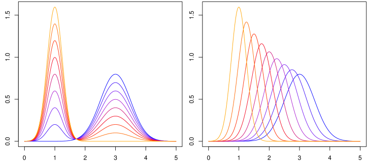
Figure 2: Densities that result from a probability average (left) or quantile average (right) of two normal distributions $N(1,0.25^{2})$ and $N(3,0.5^{2})$, as the weight on the first density varies from 1 (orange) to 0 (blue).

It seems that quantile averaging is doing something that is both like translation and scaling in probability density space. Next we explain this phenomenon precisely by recalling a classic result.

2.3.1 Shape preservation

An aggregation procedure $H$ is said to be shape-preserving if, for any location-scale family $\mathcal{P}$ (such as Normal, t, Laplace, or Cauchy) whose elements differ only by scale and location parameters, we have

$$F_{j}\in\mathcal{P},\,j=1,\ldots,p\implies F=H(F_{1},\ldots,F_{p})\in\mathcal{P}.$$

Probability averaging is clearly not shape-preserving, however, interestingly, quantile averaging is: if each $F_{j}$ a member of the same location-scale family with a base CDF $L$, then we can write $F_{j}(v)=L((v-\theta_{j})/\sigma_{j})$, thus $Q_{j}(u)=\theta_{j}+\sigma_{j}L^{-1}(u)$, so $\bar{Q}$ is still of the form $\theta+\sigma L^{-1}$ and $\bar{F}$ is also in the location-scale family. The next proposition collects this and related results from the literature.

Proposition 3 (Thomas and Ross 1980; Genest 1992)

• Quantile averaging is shape-preserving.

• Location-scale families $\mathcal{P}$ are the only ones with respect to which quantile averaging is a closed operation (meaning $F_{j}\in\mathcal{P}$, $j=1,\ldots,p$ implies $\bar{F}\in\mathcal{P}$).

• Quantile averaging is the only aggregation procedure $H$, of those satisfying (for $h$ not depending on $y$):

  $$H(F_{1},\ldots,F_{p})^{-1}(u)=h(Q_{1}(u),\ldots,Q_{p}(u)),$$

  that is shape-preserving.

Part (ii) is due to Thomas and Ross (1980). Part (iii) is due to Genest (1992), following from an elegant application of Pexider’s equation.

The parts of Proposition 3, taken together, suggest that quantile averaging is somehow “tailor-made” for shape preservation in a location-scale family—which can be seen as either a pro or a con, depending on the application one has in mind. To elaborate, suppose that in a quantile regression ensembling application, each base model outputs a normal distribution for its predicted distribution at each $x$ (with different means and variances). If the normal assumption is warranted (i.e., it actually describes the data generating distribution) then we would want our ensemble to retain normality, and quantile averaging would do exactly this. But if the normal assumption is used only as a working model, and we are looking to combine base predictions as a way to construct some flexible and robust model, then the shape-preserving property of quantile averaging would be problematic. In general, to model arbitrary distributions without imposing strong assumptions, we are therefore driven to use linear combinations of quantiles that allow different aggregation weights to be used for different quantile levels, of the form $\bar{Q}(u)=\sum_{j=1}^{p}w_{j}(u)Q_{j}(u)$.

2.3.2 Moments and sharpness

We recall an important result about moments of the distributions returned by probability and quantile averages. For a distribution $G$, we denote its uncentered moment of order $k\geq 1$ by $m_{k}(G)=\mathbb{E}_{G}[X^{k}]$, where the expectation is under $X\sim G$.

Proposition 4 (Lichtendahl et al. 2013)

• A probability and quantile average always have equal means: $m_{1}(F)=m_{1}(\bar{F})$.

• A quantile average is always sharper than a probability average: $m_{k}(\bar{F})\leq m_{k}(F)$ for any even $k\geq 2$.

Note that sharpness is only a desirable property if it does not come at the expense of calibration. With this in mind, the above result cannot be understood as a pro or con of quantile averaging without any context on calibration. That said, the relative sharpness of quantile averages to probability averages is an important general phenomenon to be aware of.

2.3.3 Tail behavior

Lastly, we study the action of quantile averaging on the tails of the subsequent probability density. Simply starting from $\bar{q}=\sum_{j=1}^{p}w_{j}q_{j}$, differentiating, and using (14), we get

$$\frac{1}{\bar{f}(\bar{Q}(u))}=\sum_{j=1}^{p}\frac{w_{j}}{f_{j}(Q_{j}(u))}.$$

That is, the probability density $\bar{f}$ at the level $u$ quantile is a (weighted) harmonic mean of the densities $f_{j}$ at their respective level $u$ quantiles. Since harmonic means are generally (much) smaller than arithmetic means, we would thus expect $\bar{f}$ to have thinner tails than $f$. The next result formalizes this. We use $g(v)=o(h(v))$ to mean $g(v)/h(v)\to 0$ as $v\to\infty$, and $g(v)\asymp h(v)$ to mean $g(v)/h(v)\to c\in(0,\infty)$ as $v\to\infty$.

Proposition 5

Assume that $p=2$, $f_{2}(v)=o(f_{1}(v))$, and the weights $w_{1},w_{2}$ are nontrivial (they lie strictly between 0 and 1). Then the density from probability averaging satisfies $f(v)\asymp f_{1}(v)$. Assuming further that $f_{1}$ is log-concave, the density from quantile averaging satisfies $\bar{f}(v)=o(f_{1}(v))$.

The proof is based on (14), and is deferred to Appendix A.4. The assumption that $f_{1}$ is log-concave for the quantile averaging result is stronger than it needs to be (as is the restriction to $p=2$), but is used to simplify exposition. Proposition 5 reiterates the importance of allowing for level-dependent weights in a linear combination of quantiles. For applications in which there is considerable uncertainty about extreme events (especially ones in which there is disagreement in the degree of uncertainty between individual base models), we would not want an ensemble to de facto inherit a particular tail behavior—whether thin or thick—but want to endow the aggregation procedure with the ability to adapt its tail behavior as needed.

3 Aggregation methods

In what follows, we describe various aggregation strategies for combining multiple conditional quantile base models into a single model. Properly trained, the ensemble should be able to account for the strengths and weaknesses of the base models and hence achieve superior accuracy to any one of them. This of course will only be possible if there is enough data to statistically identify such weaknesses and enough flexibility in the aggregation model to adjust for them.

3.1 Out-of-sample base predictions

To avoid overfitting, a standard model ensembling scheme uses out-of-fold predictions from all base models when learning ensemble weights; see, e.g., Van der Laan et al. (2007); Erickson et al. (2020). As in cross-validation, here we randomly partition the training data $\{(X_{i},Y_{i})\}_{i=1}^{n}$ into $K$ disjoint and equally-sized folds (all of our experiments use $K=5$), where the folds $\{\mathcal{I}_{k}\}_{k=1}^{K}$ form a partition of the index set $\{1,\ldots,n\}$. For each fold $\mathcal{I}_{k}$, we retrain each base model on the other folds $\{\mathcal{I}_{1},\ldots,\mathcal{I}_{K}\}\setminus\{\mathcal{I}_{k}\}$ to obtain an out-of-sample prediction at each $X_{i}$, $i\in\mathcal{I}_{k}$, denoted $\hat{g}_{j}^{-k(i)}(X_{i})$ (where we use $k(i)$ for the index of the fold containing the $i^{\text{th}}$ data point, and the superscript $-k(i)$ on the base model estimate indicates that the model is trained on folds excluding the $i^{\text{th}}$ data point). When fitting the ensemble weights, we only consider quantile predictions from each model that are out-of-sample:

$$\hat{g}_{w}(X_{i})=\sum_{j=1}^{p}w_{j}(X_{i})\cdot\hat{g}_{j}^{-k(i)}(X_{i}),\quad i=1,\ldots,n.$$ (15)

Once the ensemble weights have been learned, we make predictions at any new test point $x\in\mathcal{X}$ via (1), where the base models $\{\hat{g}_{j}\}_{j=1}^{p}$ have been fit to the full training set $\{(X_{i},Y_{i})\}_{i=1}^{n}$.

3.2 Global aggregation weighting schemes

For now, we assume that each weight is constant with respect to $x\in\mathcal{X}$, i.e., $w_{j}(x)=w_{j}$ for all $j=1,\ldots,p$. This puts us in the category of global aggregation procedures; we will turn to local aggregation procedures in the next subsection. All strategies described below can be cast in the following general form. We fit the global aggregation weights $w$ by solving the optimization problem:

$$\mathop{\mathrm{minimize}}_{w} \frac{1}{n}\sum_{i=1}^{n}\sum_{\tau\in\mathcal{T}}\psi_{\tau}\bigg{(}Y_{i}-\sum_{j=1}^{p}w_{j}\cdot\hat{g}_{j}^{-k(i)}(X_{i};\tau)\bigg{)}$$ (16)

$$\mathop{\mathrm{subject\,\,to}}\quad Aw=1,\quad w\geq 0,$$

Note that each base model prediction used in (16) is an out-of-fold prediction, as in (15). Moreover, $A$ is a linear operator that encodes the unit-sum constraint on the weights (further details on the parametrization for each case is described below):

$$Aw=\begin{cases}\sum_{j=1}^{p}w_{j}\vphantom{\big{\{}\sum_{j=1}^{p}}&\text{coarse case}\\ \big{\{}\sum_{j=1}^{p}w^{\tau}_{j}\big{\}}_{\tau\in\mathcal{T}}&\text{medium case}\\ \big{\{}\sum_{j=1}^{p}\sum_{\nu\in\mathcal{T}}w^{\tau,\nu}_{j}\big{\}}_{\tau\in\mathcal{T}}&\text{fine case}.\end{cases}$$

Lastly, in the second line of (16), we use 1 to denote the vector of all 1s (of appropriate dimension), and the constraint $w\geq 0$ is to be interpreted elementwise.

Within this framework, we can consider various weighted ensembling strategies of increasing flexibility (akin to coffee grind sizes). These were covered briefly in the introduction, and we expand on them below.

• Coarse. To each base model $\hat{g}_{j}$, we allocate a weight $w_{j}$, shared over all quantile levels. With $p$ base models, a coarse aggregator learns $p$ weights, satisfying $\sum_{j=1}^{p}w_{j}=1$. The product “$\cdot$” in (16) is just a scalar-vector product, so that ensemble prediction for level $\tau$ is

  $$\sum_{j=1}^{p}\big{(}w_{j}\cdot\hat{g}_{j}(x)\big{)}_{\tau}=\sum_{j=1}^{p}w_{j}\,\hat{g}_{j}(x;\tau).$$

  This appears to be the standard way to build weighted ensembles, including quantile ensembles, see, e.g., Nowotarski and Weron (2018); Browell et al. (2020); Zhang et al. (2020); Uniejewski and Weron (2021). However, it has clear limitations in the quantile setting, as outlined in Section 2.3. To recap, coarsely-aggregated distributions will generally have thinner tails than the thickest of the base model tails (Proposition 5), and if all base models produce quantiles according to some common location-scale family, then the coarsely-aggregated distribution will remain in this family (Proposition 3). Medium and fine strategies, described next, are free of such restrictions.

• Medium. To each base model $\hat{g}_{j}$ and quantile level $\tau$, we allocate a weight $w^{\tau}_{j}$. With $p$ base models and $m$ quantile levels, a medium aggregator learns $p\times m$ weights, satisfying $\sum_{j=1}^{p}w^{\tau}_{j}=1$ for each quantile level $\tau$. The weight assigned to each base model is a vector $w_{j}\in\mathbb{R}^{p}$, and the product “$\cdot$” in (16) is the Hadamard (elementwise) product between vectors, so that ensemble prediction for level $\tau$ is

  $$\sum_{j=1}^{p}\big{(}w_{j}\cdot\hat{g}_{j}(x)\big{)}_{\tau}=\sum_{j=1}^{p}w^{\tau}_{j}\,\hat{g}_{j}(x;\tau).$$

  This approach enables the ensemble to account for the fact that different base models may be better or worse at predicting certain quantile levels. It has been considered in quantile aggregation by, e.g., Nowotarski and Weron (2015); Maciejowska et al. (2016); Lima and Meng (2017); Tibshirani (2020).

• Fine. To each base model $\hat{g}_{j}$, output (ensemble) quantile level $\tau$, and input (base model) quantile level $\nu$, we allocate a weight $w^{\tau,\nu}_{j}$. Thus with $p$ base models and $m$ quantile levels, a fine aggregator learns $p\times m\times m$ weights, satisfying $\sum_{j=1}^{p}\sum_{\nu\in\mathcal{T}}w^{\tau,\nu}_{j}=1$ for each quantile level $\tau$. The weight assigned to each base model is a matrix $w_{j}\in\mathbb{R}^{m\times m}$, and “$\cdot$” in (16) is a matrix-vector product, so the ensemble prediction for level $\tau$ is

  $$\sum_{j=1}^{p}\big{(}w_{j}\cdot\hat{g}_{j}(x)\big{)}_{\tau}=\sum_{j=1}^{p}\sum_{\nu\in\mathcal{T}}w^{\tau,\nu}_{j}\,\hat{g}_{j}(x;\nu).$$

  This strategy presumes that for a given quantile level $\tau$, base model estimates for other quantile levels $\nu\not=\tau$ could also be useful for aggregation purposes. Note that this is particularly pertinent to a setting which some base models are poorly calibrated or produce unstable estimates for one particular quantile level. To the best of our knowledge, this type of aggregation is not common and has not been thoroughly studied in the literature.

As a way of comparing the flexibility offered by the three strategies, denote the ensemble prediction at $x$ by $\hat{g}_{w}(x)=\sum_{j=1}^{p}\big{(}w_{j}\cdot\hat{g}_{j}(x)\big{)}_{\tau}$, and note that (where we abbreviate $\operatorname*{\mathrm{range}}_{s\in S}a_{s}=[\min_{s\in S}a_{s},\,\max_{s\in S}b_{s}]$):

$$\hat{g}_{w}(x;\tau)\in\begin{cases}\operatorname*{\mathrm{range}}_{j=1,\ldots,p}\,\hat{g}_{j}(x;\tau)&\text{coarse and medium cases}\\ \operatorname*{\mathrm{range}}_{j=1,\ldots,p,\,\nu\in\mathcal{T}}\,\hat{g}_{j}(x;\nu)&\text{fine case}.\end{cases}$$

In the medium and fine cases, and any element in the respective ranges above is achieveable (by varying the weights appropriately). In the coarse case, this is not true, and $\hat{g}_{w}$ is restricted by the shape of the individual quantile functions (recall Section 2.3).

Furthermore, it is not hard to see that problem (16) is equivalent to a linear program (LP), and can be solved with any standard convex optimization toolkit. While conceptually tidy, solving this LP formulation can be overly computationally intensive at scale. In this paper, rather than relying on LP formulations, we fit global aggregation weights by optimizing (16) via stochastic gradient descent (SGD) methods, which are much more scalable to large data sets through their use of subsampled mini-batches and backpropagation in deep learning toolkits that can leverage hardware accelerators (GPUs). Outside of computational efficiency, the use of SGD also provides implicit regularization to avoid overfitting (which we can further control using early stopping). To circumvent the simplex constraints in (16), we reparametrize the weights $\{w_{j}\}_{j=1}^{p}$ using a softmax layer applied to (unconstrained) parameters $\{\phi_{j}\}_{j=1}^{p}$, which for the coarse case we can write as:

$$w=\mathtt{SoftMax}(\phi)=\bigg{\{}\frac{e^{\phi_{j}}}{\sum_{\ell=1}^{p}e^{\phi_{\ell}}}\bigg{\}}_{j=1}^{p}.$$

The other cases (medium and fine) follow similarly.

Yet another advantage of using SGD and deep learning toolkits to solve (16) is that this extends more fluidly to the setting of local aggregation weights, which we described next.

3.3 Local aggregation via neural networks

To fit local aggregation weights that vary with $x\in\mathcal{X}$, we use a neural network approach. For concreteness, we describe the procedure in the context of fine aggregation weights, and the same idea applies to the other cases (coarse and medium) as well. We will refer to the local-fine approach, described below, as deep quantile aggregation or DQA.

To fit weight functions $w^{\tau,\nu}_{j}:\mathcal{X}\to\mathbb{R}$, we model these jointly over all base models $j\in\{1,2,\ldots,p\}$ and all pairs of quantile levels $(\tau,\nu)\in\mathcal{T}\times\mathcal{T}$ using a single neural network $G$. All but the last layer of $G$ forms a feature extractor $f_{\theta}:\mathcal{X}\rightarrow\mathbb{R}^{d}$ that maps input feature values $x\in\mathcal{X}$ to a hidden representation $h\in\mathbb{R}^{d}$. In our experiments, we take $f_{\theta}$ to be a standard feed-forward network parametrized by $\theta$. The last layer of $G$ is defined, for each output quantile level $\tau\in\mathcal{T}$, by a matrix $W^{\tau}\in\mathbb{R}^{pm\times d}$ that maps the hidden representation $h$, followed by a softmax operation (to ensure the simplex constraints are met), to fine aggregation weights $w^{\tau}(x)\in\mathbb{R}^{pm}$, as in:

$$w^{\tau}(x)=G(x;\theta,W^{\tau})=\mathtt{SoftMax}\big{(}W^{\tau}f_{\theta}(x)\big{)},\quad\tau\in\mathcal{T}.$$ (17)

The parameters $\theta$ and $\{W^{\tau}\}_{\tau\in\mathcal{T}}$ can be jointly optimized via SGD, applied to the optimization problem:

$$\mathop{\mathrm{minimize}}_{\theta,\,\{W^{\tau}\}_{\tau\in\mathcal{T}}}\;\frac{1}{n}\sum_{i=1}^{n}\sum_{\tau\in\mathcal{T}}\psi_{\tau}\bigg{(}Y_{i}-\sum_{j=1}^{p}\sum_{\nu\in\mathcal{T}}G(x;\theta,W^{\tau})_{j,\nu}\,\hat{g}^{-k(i)}_{j}(X_{i};\nu)\bigg{)}.$$ (18)

Note that there are no explicit constraints because the softmax parametrization in (17) implicitly fulfills the appropriate constraints.

Why would we want to move from using global aggregation weights (16), which do not depend on the feature values $x$, to using local aggregation weights (17), (18), which do? Aside from the general perspective of increasing model flexibility, local weights can be motivated by the observation that, in any given problem setting, it may well be the case that that certain constituent models perform better (output more accurate quantile estimates) in some parts of the feature space, while others perform better in other parts. In such cases, a local aggregation scheme will be able to adapt its weights accordingly, whereas a global scheme will not, and will be stuck with attributing some global level of preference between the models.

3.4 Interpreting the local aggregation scheme

We can interpret our proposal in (17), (18) as a mixture of experts ensemble (Jacobs et al., 1991) where the gating network $G$ emits predictions about which “experts” will be most accurate for any particular $x$. In the local-fine setting (DQA), the “experts” correspond to estimates of individual quantiles from individual base models, and we define a separate gating scheme for each target quantile level $\tau$.

We can also view our local-fine aggregator through the lens of an attention mechanism (Bahdanau et al., 2015), which adaptively attends to the different quantile estimates from each base model, and uses a different attention map for each $\tau$ and each $x$. In terms of the architecture design, we use a representation of the tuple $(\tau,x)$ both as a key and as a query. The individual quantiles $\hat{g}_{j}(x;\tau)$ are then used as values in the (query, key, value) mechanism commonly used.

Visualizing these attention maps—see Figures 4 and 4—can help address natural questions, e.g., for any particular $x$ and $\tau$, which base estimates are most useful? Or, how do estimates at different quantile levels interact with each other to achieve accuracy in the ensemble? While this conveys only qualitative information, we note that interpretations such as these would be far more difficult to obtain for nonlinear aggregators like stacked ensembles (Wolpert, 1992).

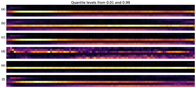
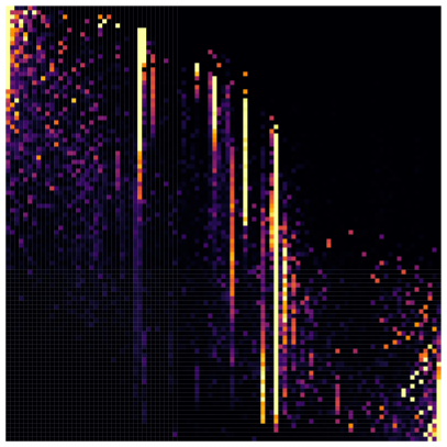
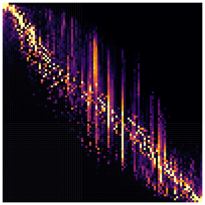
Figure 3: Heatmaps of aggregation weights fit by the local-medium aggregator to the concrete data set, at 6 different input feature values. Each heatmap in (a)–(f) corresponds to a particular input feature value $x$. Its rows correspond to the $p=6$ base models, and columns to the $m=99$ quantile levels. A black color means that a given base prediction is essentially ignored by the aggregator. We can see that for different $x_{i}$ the algorithm chooses different base models but also that it then mostly uses the estimates of these base models in a consistent fashion across quantile levels.

Figure 4: Heatmaps of aggregation weights fit by the local-fine (DQA) aggregator to the concrete data set (left) and the power data set (right). In the current fine setting, we have one $m\times m=99\times 99$ weight matrix per base model; the heatmaps have therefore been averaged over the $p=6$ base models. Their rows correspond to the output quantiles (for the aggregator), and the columns to the input quantiles (from the base model). The right heatmap displays clear concentration around the diagonal: here each input quantile is on average the most reliable estimate used to define its corresponding output quantile. This is much less true on the left, which also has more pronounced vertical “streaks”: output quantiles use input quantiles from many neighboring quantile levels. The left heatmap also has notably more dispersion in the tails.

3.5 New base model: deep quantile regression

Finally, we remark that the optimization in (18) can be used to itself define a standalone neural network quantile regressor, which we refer to as deep quantile regression or DQR. This is given by taking $p=1$ in (18) with a trivial base model that outputs $\hat{g}_{1}(x;\tau)=1$, for any $x$ and $\tau$. DQR can be useful as a base model (to feed into an aggregation method like DQA), and will be used as a point of comparison and/or illustration at various points in what follows. For example, Figure 5 illustrates DQR on a real data set.

4 Quantile noncrossing

Here we discuss methods for enforcing quantile noncrossing in the predictions produced by the aggregation methods from the last section. We combine and extend the ideas introduced in Section 2.2.

4.1 Crossing penalty and quantile buffering

As an alternative to enforcing hard noncrossing constraints during training, as in (10), we consider a crossing penalty of the form:

$$\rho(g)=\sum_{x\in\mathcal{X}_{0}}\sum_{\tau<\tau^{\prime}}\big{(}g(x;\tau)-g(x;\tau^{\prime})+\delta_{\tau,\tau^{\prime}}\big{)}_{+},$$ (19)

where $a_{+}=\max\{a,0\}$, and $\delta_{\tau,\tau^{\prime}}\geq 0$, for $\tau<\tau^{\prime}$ are constants (not depending on $x$) that encourage a buffer between pairs of quantiles at different quantile levels. In the simplest case, we can reduce this to just a single margin $\delta_{\tau,\tau^{\prime}}=\delta$ across all quantile levels, that we can tune as a hyperparameter (e.g., using a validation set). We will cover a slightly more advanced strategy shortly, for fitting adaptive margins which vary with quantile levels (as well as the training data at hand).

The advantage of using a penalty (19) over constraints is primarily computational: we can add it to the criterion defining the aggregation model, and we can still use SGD for optimization. Note that the penalty is applied at the ensemble level, to $g=\hat{g}_{w}=\sum_{j=1}^{p}w_{j}\cdot\hat{g}_{j}$; to be precise, the global optimization (16) becomes

$$\mathop{\mathrm{minimize}}_{w} \frac{1}{n}\sum_{i=1}^{n}\sum_{\tau\in\mathcal{T}}\psi_{\tau}\bigg{(}Y_{i}-\sum_{j=1}^{p}w_{j}\cdot\hat{g}_{j}^{-k(i)}(X_{i};\tau)\bigg{)}+\lambda\,\rho\bigg{(}\sum_{j=1}^{p}w_{j}\cdot\hat{g}_{j}\bigg{)}$$ (20)

$$\mathop{\mathrm{subject\,\,to}}\quad Aw=1,\quad w\geq 0,$$

where $\lambda\geq 0$ is a hyperparameter to be tuned. The modification of the local optimization (18) to include the penalty term is similar. Figure 5 gives an illustration of the crossing penalty in action.

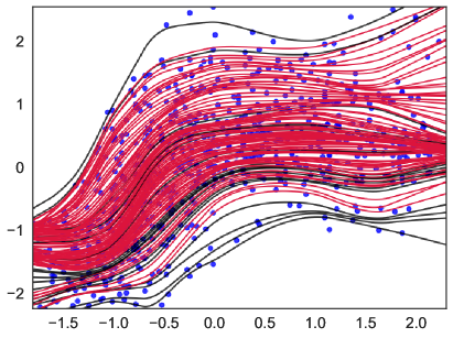
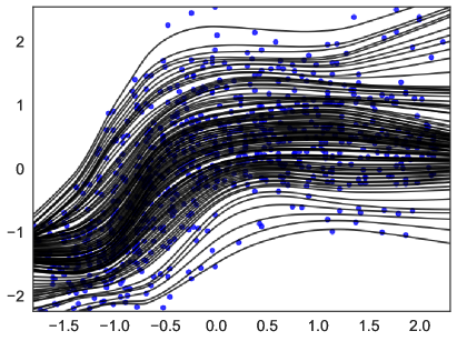
Figure 5: Conditional quantile estimates fit by a neural network quantile regressor (DQR) to the bone mineral data set, used in Takeuchi et al. (2006), where $X$ is univariate. The left panel displays estimates that were fit without any crossing penalty or isotonization operator, and the right panel displays estimates fit using the crossing penalty (19) and post sorting. (This is the simplest combination among all the methods that we consider to address quantile crossing.) Crossing quantile curves are highlighted in red.

4.1.1 Adaptive margins

One of the problems with choosing a fixed margin $\delta$ (of using the reduction $\delta_{\tau,\tau^{\prime}}=\delta$ for all $\tau,\tau^{\prime}$) is that it may not accurately reflect the scale or shape of the quantile gaps in the data at hand. We propose the following heuristic for tuning margin parameters $\delta_{\tau,\tau^{\prime}}$, over all pairs of distinct levels $\tau<\tau^{\prime}$. We begin with any pilot estimator of the conditional mean or median of $Y|X$, call it $\hat{g}_{0}$, and form residuals $R_{i}=Y_{i}-\hat{g}_{0}(X_{i})$, $i=1,\ldots,n$. The closer these residuals are to the true error distribution, of $Y-\mathbb{E}(Y|X)$ (or similar for the median), the better. Thus we typically want to use cross-validation residuals for this pilot step. We then take, for each $\tau<\tau^{\prime}$, the margin to be

$$\delta_{\tau,\tau^{\prime}}=\delta_{0}\big{(}Q_{\tau^{\prime}}(\{R_{i}\}_{i=1}^{n})-Q_{\tau}(\{R_{i}\}_{i=1}^{n})\big{)}_{+}.$$ (21)

where $Q_{\tau}$ gives the empirical level $\tau$ quantile of its argument. The motivation behind the proposal in (21) is that $Q_{\tau^{\prime}}(\{R_{i}\}_{i=1}^{n})-Q_{\tau}(\{R_{i}\}_{i=1}^{n})$ is itself the gap between quantile estimates from a basic but properly (monotonically) ordered quantile regressor, namely, that defined by:

$$\hat{g}_{0}(x;\tau)=\hat{g}_{0}(x)+Q_{\tau}(\{R_{i}\}_{i=1}^{n}),\quad x\in\mathcal{X},\,\tau\in\mathcal{T}.$$

We note that $\delta_{0}\geq 0$ in (21) is a single hyperparameter to be tuned. In our experiments, we take the pilot estimator to be the simple average of base model predictions at the median, $\hat{g}_{0}(x)=\frac{1}{p}\sum_{j=1}^{p}\hat{g}_{j}(x;0.5)$, and we use the same cross-validation scheme for the base models as in Section 3.1 to produce out-of-fold residuals $R_{i}$, $i=1,\ldots,n$ around $\hat{g}_{0}$, that are used in (21).

4.2 Isotonization: post hoc and end-to-end

Next we consider different isotonization operators that can be used in conjunction with the crossing penalty in (19). This is important because it will guarantee quantile noncrossing for the ensemble predictions at all points $x\in\mathcal{X}$, as in (9), whereas the crossing penalty alone is not sufficient to ensure this. The added benefit of this approach is that we are able to satisfy the constraint at out-of-sample points without having to invest unreasonable amounts of function complexity into the model, simply by applying isotonization as a form of prior knowledge (see Le et al. 2006 for a detailed general discussion of this aspect).

Generally, an isotonization operator $\mathcal{S}$ can be used in one of two ways. The first is post hoc, as explained in Section 2.2, where we simply apply it to quantile predictions after the ensemble $\hat{g}=\sum_{j=1}^{p}\hat{w}_{j}\cdot\hat{g}_{j}$ has been trained, as in (11). The second way is end-to-end, where $\mathcal{S}$ gets used a layer in training, and we now solve, instead of (20),

$$\mathop{\mathrm{minimize}}_{w} \frac{1}{n}\sum_{i=1}^{n}\sum_{\tau\in\mathcal{T}}\psi_{\tau}\Bigg{(}Y_{i}-\bigg{[}\mathcal{S}\bigg{(}\sum_{j=1}^{p}w_{j}\cdot\hat{g}_{j}^{-k(i)}(X_{i})\bigg{)}\bigg{]}_{\tau}\Bigg{)}+\lambda\,\rho\bigg{(}\sum_{j=1}^{p}w_{j}\cdot\hat{g}_{j}\bigg{)}$$ (22)

$$\mathop{\mathrm{subject\,\,to}}\quad Aw=1,\quad w\geq 0,$$

where we denote by $[\mathcal{S}(v)]_{\tau}$ the element of $\mathcal{S}(v)$ corresponding to a quantile level $\tau$. The modification for the local aggregation problem is similar. For predictions, we still post-apply $\mathcal{S}$, as in (11).

One might imagine that the end-to-end approach can help predictive accuracy, since in training we are leveraging the knowledge of what we will be doing at prediction time (applying $\mathcal{S}$). Furthermore, by treating $\mathcal{S}$ as a differentiable layer, we can still seamlessly apply SGD for optimization (end-to-end training). Note that sorting (12) and isotonic projection (13) are almost everywhere differentiable (they are in fact almost everywhere linear maps). We will propose an additional isotonization operator shortly that is also almost everywhere differentiable, and particularly convenient to implement in modern deep learning toolkits.

To be clear, the end-to-end approach is not free of downsides; while sorting and isotonic projection are guaranteed to improve WIS when applied post hoc (Proposition 2), the same cannot be said when they are used end-to-end. Thus we give up on a formal guarantee, to potentially gain accuracy in practice.

4.2.1 Min-max sweep

In addition to sorting (12) and isotonic projection (13), we propose and investigate a simple isotonization operator that we call the min-max sweep. It works as follows: starting at the median, it makes two outward sweeps: one upward and one downward, where it replaces each value with a cumulative max (upward sweep) or cumulative min (downward sweep). To be more precise, if we have sorted quantile levels $\tau_{1}<\cdots<\tau_{m}$ with $\tau_{m_{0}}=0.5$, and corresponding values $v_{1},\ldots,v_{m}$, then we define the min-max sweep operator according to:

$$\mathtt{MinMaxSweep}(v)_{k}=\begin{cases}v_{k}&k=m_{0}\\ \max\{v_{k},\,\mathtt{MinMaxSweep}(v)_{k-1}\}&k=m_{0}+1,\ldots,m\\ \min\{v_{k},\,\mathtt{MinMaxSweep}(v)_{k+1}\}&k=m_{0}-1,\ldots,1.\end{cases}$$ (23)

Like sorting and isotonic projection, the min-max sweep is almost everywhere a linear map, and thus almost everywhere differentiable. The primary motivation for it is that it can be implemented highly efficiently in modern deep learning frameworks via cumulative max and cumulative min functions—these are vectorized operations that can be efficiently applied in parallel over a mini-batch, in each iteration of SGD (when it is used in an end-to-end manner). Unlike sorting and isotonic projection, however, it is not guaranteed to improve WIS (Proposition 2) when applied in post.

5 Conformal calibration

Informally, a conditional quantile estimator is said to be calibrated provided that its quantile estimates have the appropriated nominal one-sided coverage, for example, an estimated 90% quantile covers the target from above 90% of the time, and the same for the other quantile levels being estimated. Equivalently, we can view this in terms of central prediction intervals: the interval whose endpoints are given by the estimated 5% and 95% quantiles covers the target 90% of the time. Formally, let $\hat{g}$ be an estimator trained on samples $(X_{i},Y_{i})$, $i=1,\ldots,n$, with $\hat{g}(x;\tau)$ denoting the estimated level $\tau$ quantile of $Y|X=x$. Assume that the set of quantile levels $\mathcal{T}$ being estimated is symmetric around 0.5, so we can write it as $\mathcal{T}=\cup_{\alpha\in\mathcal{A}}\{\alpha/2,1-\alpha/2\}$. Then $\hat{g}$ is said to be calibrated, provided that for every $\alpha\in\mathcal{A}$, we have

$$\mathbb{P}\Big{(}Y_{n+1}\in\Big{[}\hat{g}(X_{n+1};{\alpha}/{2}),\,\hat{g}(X_{n+1};1-{\alpha}/{2})\Big{]}\Big{)}=1-\alpha,$$ (24)

where $(X_{n+1},Y_{n+1})$ is a test sample, assumed to be i.i.d. with the training samples $(X_{i},Y_{i})$, $i=1,\ldots,n$. To be precise, the notion of calibration that we consider in (24) is marginal over everything: the training set and the test sample. We remark that a stronger notion of calibration, which may often be desirable in practice, is calibration conditional on the test feature value:

$$\mathbb{P}\Big{(}Y_{n+1}\in\Big{[}\hat{g}(X_{n+1};{\alpha}/{2}),\,\hat{g}(X_{n+1};1-{\alpha}/{2})\Big{]}\,\Big{|}\,X_{n+1}=x\Big{)}=1-\alpha,\quad x\in\mathcal{X}.$$ (25)

Conditional calibration, as in (25), is actually impossible to achieve in a distribution-free sense; see Lei and Wasserman (2014); Vovk (2012); Barber et al. (2021a) for precise statements and developments. Meanwhile, marginal calibration (24) is possible to achieve using conformal prediction methodology, without assuming anything about the joint distribution of $(X,Y)$. The definitive reference on conformal prediction is the book by Vovk et al. (2005); see also Lei et al. (2018), which helped popularize conformal methods in the statistics and machine learning communities. The conformal literature is by now somewhat vast, but we will only need to discuss a few parts of it that are most relevant to calibration of conditional quantile estimators.

In particular, we very briefly review conformalized quantile regression or CQR by Romano et al. (2019) and CV+ by Barber et al. (2021b). We then discuss how these can be efficiently applied in combination to any of the quantile aggregators studied in this paper.

5.1 CQR

We first describe CQR in a split-sample setting. Suppose that we have reserved a subset indexed by $\mathcal{I}_{1}\subseteq\{1,\ldots,n\}$ as the proper training set, and $\mathcal{I}_{2}=\{1,\ldots,n\}\setminus\mathcal{I}_{1}$ as the calibration set. (Extending this to a cross-validation setting, via the CV+ method, is discussed next.) In this split-sample setting, CQR from Romano et al. (2019) can be explained as follows.

1. First, fit the quantile estimator $\hat{g}^{\mathcal{I}_{1}}$ on the proper training set $\{(X_{i},Y_{i}):i\in\mathcal{I}_{1}\}$.

2. Then, for each $\alpha\in\mathcal{A}$, compute lower and upper residuals on the calibration set,

   $$R^{-}_{i,\alpha}=\hat{g}^{\mathcal{I}_{1}}(X_{i};\alpha/2)-Y_{i}\quad\text{and}\quad R^{+}_{i,\alpha}=Y_{i}-\hat{g}^{\mathcal{I}_{1}}(X_{i};1-\alpha/2),\quad i\in\mathcal{I}_{2}.$$

3. Finally, adjust (or conformalize) the original estimates based on residual quantiles, yielding for $\alpha\in\mathcal{A}$ and $x\in\mathcal{X}$,

   $$\tilde{g}(x;\alpha/2) =\hat{g}^{\mathcal{I}_{1}}(x;\alpha/2)-\tilde{Q}_{1-\alpha/2}\big{(}\{R^{-}_{i,\alpha}:i\in\mathcal{I}_{2}\}\big{)},$$ (26)

   $$\tilde{g}(x;1-\alpha/2) =\hat{g}^{\mathcal{I}_{1}}(x;1-\alpha/2)+\tilde{Q}_{1-\alpha/2}\big{(}\{R^{+}_{i,\alpha}:i\in\mathcal{I}_{2}\}\big{)},$$

   where $\tilde{Q}_{\tau}$ is a slightly modified empirical quantile function, giving the empirical level $\lceil\tau(n_{2}+1)\rceil/n_{2}$ quantile of its argument, with $n_{2}=|\mathcal{I}_{2}|$.

A cornerstone result in conformal prediction theory (see Theorems 1 and 2 in Romano et al. (2019) for the application of this result to CQR) says that for any estimator, its conformalized version in (26) has the finite-sample marginal coverage guarantee

$$\mathbb{P}\Big{(}Y_{n+1}\in\Big{[}\tilde{g}(X_{n+1};{\alpha}/{2}),\,\tilde{g}(X_{n+1};1-{\alpha}/{2})\Big{]}\Big{)}\geq 1-\alpha.$$ (27)

In fact, the coverage of the level $1-\alpha$ central prediction interval is also upper bounded by $1-\alpha+1/(n_{2}+1)$, provided that the residuals are continuously distributed (i.e., there are almost surely no ties).

5.2 CV+

Now we describe how to extend CQR to a cross-validation setting. Let $\{I_{k}\}_{k=1}^{K}$ denote a partition of $\{1,\ldots,n\}$ into disjoint folds. We can map steps 1–3 used to produce the CQR correction in (26) onto the CV+ framework of Barber et al. (2021b), as follows.

1. First, for each fold $k=1,\ldots,K$, fit the quantile estimator $\hat{g}^{-k}$ on all data points but those in the $k^{\text{th}}$ fold, $\{(X_{i},Y_{i}):i\notin\mathcal{I}_{k}\}$.

2. Then, for each $i=1,\ldots,n$ and each $\alpha\in\mathcal{A}$, compute lower and upper residuals on the calibration fold $k(i)$ (where $k(i)$ denotes the index of the fold containing the $i^{\text{th}}$ data point),

   $$R^{-}_{i,\alpha}=\hat{g}^{-k(i)}(X_{i};\alpha/2)-Y_{i}\quad\text{and}\quad R^{+}_{i,\alpha}=Y_{i}-\hat{g}^{-k(i)}(X_{i};1-\alpha/2),\quad i\in\mathcal{I}_{k(i)}.$$

3. Finally, adjust (or conformalize) the original estimates based on residual quantiles, yielding for $\alpha\in\mathcal{A}$ and $x\in\mathcal{X}$,

   $$\tilde{g}(x;\alpha/2) =\tilde{Q}^{-}_{1-\alpha/2}\Big{(}\big{\{}\hat{g}^{-k(i)}(x;\alpha/2)-R^{-}_{i,\alpha}:i\in k(i)\big{\}}\Big{)},$$ (28)

   $$\tilde{g}(x;1-\alpha/2) =\tilde{Q}^{+}_{1-\alpha/2}\Big{(}\big{\{}\hat{g}^{-k(i)}(x;1-\alpha/2)+R^{+}_{i,\alpha}:i\in k(i)\big{\}}\Big{)},$$

   where now $\tilde{Q}^{-}_{\tau},\tilde{Q}^{+}_{\tau}$ are modified lower and upper level $\tau$ empirical quantiles: for any set $Z$, we define $\tilde{Q}^{+}_{\tau}(Z)$ to be the level $\lceil\tau(|Z|+1)\rceil/|Z|$ empirical quantile of $Z$, and $\tilde{Q}^{-}_{\tau}(Z)=-\tilde{Q}^{+}(-Z)$.

According to results from Barber et al. (2021b) and Vovk et al. (2018) (see Theorem 4 in Barber et al. (2021b) for a summary), for any estimator, its conformalized version in (28) has the finite-sample marginal coverage guarantee

$$\mathbb{P}\Big{(}Y_{n+1}\in\Big{[}\tilde{g}(X_{n+1};{\alpha}/{2}),\,\tilde{g}(X_{n+1};1-{\alpha}/{2})\Big{]}\Big{)} \geq 1-2\alpha-\min\bigg{\{}\frac{2(1-1/K)}{n/K+1},\,\frac{1-K/n}{K+1}\bigg{\}}$$ (29)

$$\geq 1-2\alpha-\sqrt{2/n}.$$

We can see that the guarantee from CV+ in (29) is weaker than that in (27) from sample-splitting, though CV+ has the advantage that it utilizes each data point for both training and calibration purposes, and can often deliver shorter conformalized prediction intervals as a result. Moreover, Barber et al. (2021b) argue that for stable estimation procedures, the empirical coverage from CV+ is closer to $1-\alpha$ (and provide some theory to support this as well).

5.3 Nested implementation for quantile aggregators

We discuss the application of CQR and CV+ to calibrate the quantile aggregation models developed in Section 3 and 4. An additional level of complexity in this application arises because the quantile aggregation model is itself built using cross-validation: recall, as discussed in Section 3.1, that the aggregation weights are trained using out-of-sample (out-of-fold) predictions from the base models. Thus, application of CV+ here requires a nested cross-validation scheme, where in the inner loop, the aggregator is trained using cross-validation (for the base model predictions), and in the outer loop, the calibration residuals are computed for the ultimate conformalization step.

In order to make this as computationally efficient as possible, we introduce a particular nesting scheme that reduces the number of times base models are trained by roughly a factor of 2. We first pick a number of folds $K$ for the outer loop, and define folds $\mathcal{I}_{k}$, $k=1,\ldots,K$. Then for each $k=1,\ldots,K$, we fit the quantile aggregation model $\hat{g}_{w}^{-k}$ on $\{(X_{i},Y_{i}):i\notin\mathcal{I}_{k}\}$ (using any one of the approaches described in Sections 3 and 4), with the key idea being how we implement the inner cross-validation loop to train the base models: we use folds $\mathcal{I}_{\ell}$, $\ell\not=k$ for this inner loop, so that we can later avoid having to refit the base models when the roles of $k$ and $\ell$ are reversed. To see more clearly why this is the case, we describe the procedure in more detail below.

1. For $k=1,\ldots,K$:

   1. For $\ell\not=k$, train each base model $\hat{g}_{j}^{-k,\ell}$ on $\{(X_{i},Y_{i}):i\notin\mathcal{I}_{k}\cup\mathcal{I}_{\ell}\}$.

   2. Train the aggregation weights $w$ on $\{(X_{i},Y_{i}):i\notin\mathcal{I}_{k}\}$ (using the base model predictions $\hat{g}_{j}^{-k,\ell}(X_{i})$ from Step a), to produce the aggregator $\hat{g}_{w}^{-k}$.

   3. Compute lower and upper calibration residuals of $\hat{g}_{w}^{-k}$ on $\{(X_{i},Y_{i}):i\in\mathcal{I}_{k}\}$, as in Step 2 of CV+.

2. Conformalize original estimates using residual quantiles, as in Step 3 of CV+.

The computational savings comes from observing that $\hat{g}_{j}^{-k,\ell}=\hat{g}_{j}^{-\ell,k}$: the base model we train when $k$ is the calibration fold and $\ell$ is the validation fold is the same as that we would train when the roles of $k$ and $\ell$ are reversed. Therefore we only need to train each base model in Step 1a, across all iterations of the outer and inner loops, a total of $K(K-1)/2$ times, as opposed to $K(K-1)$ times if we were ignorant to this fact (or $K^{2}$ times, the result of a more typical nested $K$-fold cross-validation scheme).

6 Empirical comparisons

We provide a broad empirical comparison of our proposed quantile aggregation procedures as well as many different established regression and aggregation methods. We examine 34 data sets in total: 8 from the UCI Machine Learning Repository (Dua and Graff, 2017) and 26 from the AutoML Benchmark for Regression from the Open ML Repository (Vanschoren et al., 2013). These have served as popular benchmark repositories in probabilistic deep learning and uncertainty estimation, see, e.g., Lakshminarayanan et al. (2017); Mukhoti et al. (2018); Jain et al. (2020); Fakoor et al. (2020). To the best of our knowledge, what follows is the most comprehensive evaluation of quantile regression/aggregation methods published to date.

6.1 Training, validation, and testing setup

For each of the 34 data sets studied, we average all results over 5 random train-validation-test splits, of relative size 72% (train), 18% (validation), and 10% (test). We adopt the following workflow for each data set.

1. Standardize the feature variables and response variable on the combined training and validation sets, to have zero mean and unit standard deviation.

2. Fit the base models on the training set.

3. Find the best hyperparameter configuration for each base model by minimizing weighted interval score (WIS) on the validation set. Fix these henceforth.

4. Divide the training set into 5 random folds. Record out-of-fold (OOF) predictions for each base model; that is, for fold $k$, we fit each base model $\hat{g}_{j}^{-k}$ by training on data from all folds except $k$, and use it to produce $\hat{g}_{j}^{-k}(X_{i})$ for each $i$ such that $k(i)=k$.

5. Fit the aggregation models on the training set, using the OOF base predictions from the last step.

6. Find the best hyperparameter configuration for each aggregation model by again minimizing validation WIS. Fix these henceforth.

7. Report the test WIS for each aggregation model (making sure to account for the initial standardization step, in the test set predictions).

All base and aggregation models are fit using $m=99$ levels, $\mathcal{T}=\{0.01,0.02,\ldots,0.99\}$; the specific base and aggregation models we consider are described below. The initial standardization step is convenient for hyperparameter tuning. For more details on hyperparameter tuning, see Appendix B.1 and B.2.

6.2 Base models

We consider $p=6$ quantile regression models as base models for the aggregators, described below, along with the abbreviated names we give them henceforth. The first three are neural network models with different architectures and objectives. More details are given in Appendix B.1.

1. Conditional Gaussian network (CGN, Lakshminarayanan et al., 2017).

2. Simultaneous quantile regression (SQR, Tagasovska and Lopez-Paz, 2019);

3. Deep quantile regression (DQR), which falls naturally out of our framework, as explained in Section 3.3.

4. Quantile random forest (RandomForest, Meinshausen, 2006).

5. Extremely randomized trees (ExtraTrees, Geurts et al., 2006).

6. Quantile gradient boosting (LightGBM, Ke et al., 2017).

6.3 Aggregation models

We study 4 aggregation models outside of the ones defined in our paper, described below, along with their abbreviated names. More details are given in Appendix B.2.

1. Average: a straight per-quantile average of base model predictions.

2. Median: a straight per-quantile median of base model predictions.

3. Quantile regression averaging (QRA, Nowotarski and Weron, 2015).

4. Factor QRA (FQRA, Maciejowska et al., 2016).

The rest of this section proceeds as follows. We first discuss the performance of the local-fine aggregator from our framework in Section 3, called DQA, to other methods (all base models, and the other aggregators defined outside of this paper). In the subsections that follow, we move on to a finer analysis, comparing the different weighted ensembling strategies to each other, comparing the different isotonization approaches to each other, and evaluating the gains in calibration made possible by conformal prediction methodology.

6.4 Continuation of Figure 1

Recall that in Figure 1, we already described some results from our empirical study, comparing DQA to all other methods. To be precise, for DQA—in Figure 1, here, and henceforth—we use the simplest strategy to ensure quantile noncrossing among the options discussed in Section 4: the crossing penalty along with post sorting (CrossPenalty + PostSort in the notation that we will introduce shortly). To give an aggregate view of the same results, Figure 7 shows the average relative WIS over all data sets. Relative WIS is the ratio of the WIS of given method to that of DQA, hence 1 indicates equal performance to DQA, and larger numbers indicate worse performance. (Standard error bars are also drawn.) These results clearly show the favorable average-case performance of DQA, to complement the per-data-set view in Figure 1. We can also see that QRA and FQRA are runners up in terms of average performance; while they are fairly simple aggregators, based on quantile linear regression, they use inputs here the predictions from flexible base models. Going back to the results in Figure 1, it is worth noting that there are data sets for which QRA and FQRA perform clearly worse than DQA (up to 50% worse, a relative factor of 1.5), but none where they perform better. In Appendix B.3, we provide an alternative visualization of these same results (differences in WIS rather than ratios of WIS).

6.5 Comparing ensembling strategies

Now we compare different ensembling strategies of varying flexibility, as discussed in Section 3. Recall that we have two axes: global or local weighting; and coarse, medium, or fine parameterization. This gives a total of 6 approaches, which we denote by global-coarse, global-medium, and so on. Figure 7 displays the relative WIS of each method to global-fine per data set (left panel), and the average relative WIS over all data sets (right panel). The data sets here and henceforth are indexed by increasing PVE, as in Figure 1. We note that global-fine is like a “middle man” in terms of its flexibility, among the 6 strategies considered. The overall trend in Figure 7 is that greater flexibility leads to better performance, especially for larger PVE values.

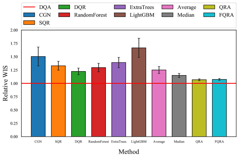
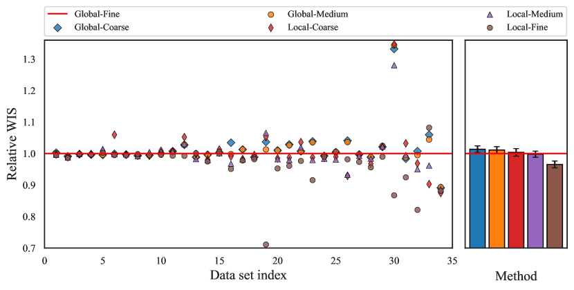
Figure 6: Average relative WIS over all data sets for deep quantile aggregation (DQA) and various quantile regression methods. The per-data-set results are given in Figure 1. Numbers larger than 1 indicate a worse average performance than DQA. We see that DQA performs the best overall, and QRA and FQRA are somewhat close runners up.

Figure 7: Comparing the relative WIS of various ensembling strategies to global-fine. The left panel shows the relative WIS per data set (ordered by increasing PVE), and the right panel shows the average relative WIS over all data sets. In general, the more flexible aggregation strategies tend to perform better, and local-fine (DQA) performs the best overall.

6.6 Comparing isotonization approaches

We compare the various isotonization approaches discussed in Section 4, applied to DQA. In Figure 8, the legend label “none” refers to DQA without any penalty and any isotonization operator; all WIS scores are computed relative to this method. CrossPenalty and AdaptCrossPenalty, respectively, denote the crossing penalty and adaptive cross penalty from Section 4.1. PostSort and GradSort, respectively, denote the sorting operator applied in post-processing and in training (see (22) for how this works in the global models), as described in Section 4.2. We similarly use PostPAVA, GradPAVA, and so on. Lastly, we use “+” to denote the combination of a penalty and isotonization operator, as in CrossPenalty + PostSort. The main takeaway from Figure 8 is that all of the considered methods improve upon “None”. However, it should be noted that these are second-order improvements in relative WIS compare to the much larger first-order improvements in Figures 1 and 7, of DQA over base models and other aggregators—compare the y-axis range in Figure 8 to that in Figures 1 and 7.

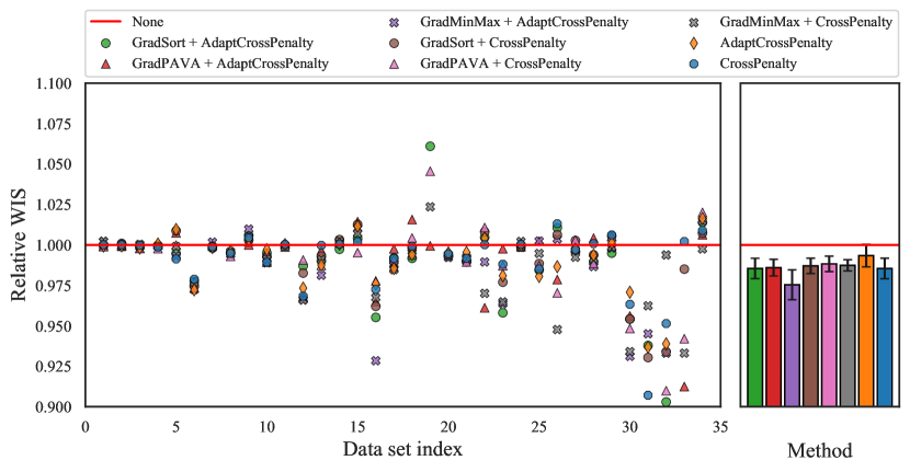
Figure 8: Comparing the relative WIS of various isotonization strategies on top of pure DQA, with no penalty and no isotonization operator (“none”). The display is as in Figure 7 (individual results per data set on left panel, averaged results on right panel). We can see that all isotonization methods offer consistent but small improvements on “none”, with AdaptCrossPenalty + GradMinMax achieving the best average-case performance.

A second takeaway from Figure 8 might be to generally recommend AdaptCrossPenalty + GradMinMax for future aggregation problems, which had the best average performance across our empirical suite. That said, given the small relative improvement this offers, we generally stick to using the simpler CrossPenalty + PostSort in the current paper.

Finally, Figure 9 gives an empirical verification of Proposition 2, which recall, showed that sorting and PAVA applied in post-processing can never make WIS worse. We can see that for each of the 34 data sets, combining PostSort or PostPAVA with CrossPenalty (left panel) or AdaptCrossPenalty (right panel) never hurts WIS, and occasionally improves it. This is not true for PostMinMax, as we can see that PostMinMax hurts WIS in a few data sets across the panels, the most noticeable instance being data set 19 on the left.

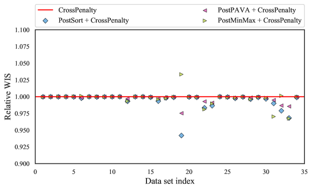
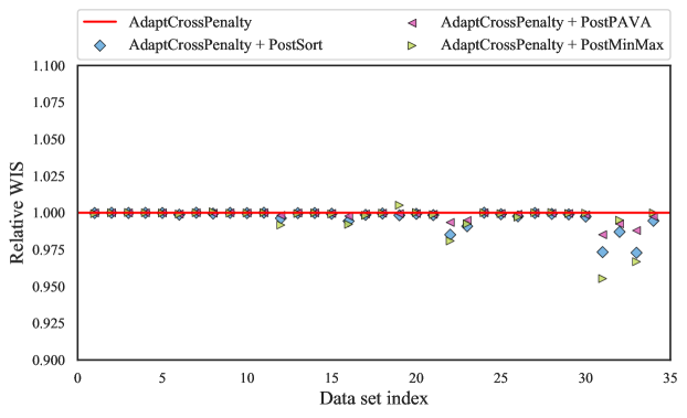
Figure 9: Comparing post isotonization strategies applied on top of CrossPenalty (shown in the top figure), and AdaptCrossPenalty (shown in the bottom figure). As we can see in either figure, PostSort and PostPAVA can only improve WIS; verifying Proposition 2. This is not true of PostMinMax, the most noticeable example being data set 19 in the top figure.

6.7 Evaluating conformal calibration

We examine the CQR-CV+ method from Section 5 applied to DQA, to adjust its central prediction intervals to have proper coverage. Figures 11 and 11 summarize empirical coverage and interval length at the nominal 0.8 coverage level, respectively. Note that the results for other nominal levels are similar. Here, the coverage and length of a quantile regressor $\hat{g}$ at level $1-\alpha$ are defined as

$$\frac{1}{m}\sum_{i=1}^{m}1\Big{\{}\hat{g}(X^{*}_{i};\alpha/2)\leq Y^{*}_{i}\leq\hat{g}(x_{i};1-\alpha/2)\Big{\}},$$

$$\frac{1}{m}\sum_{i}^{m}\Big{[}\hat{g}(X^{*}_{i};1-\alpha/2)-\hat{g}(X^{*}_{i};\alpha/2)\Big{]},$$

respectively, where $(X^{*}_{i},Y^{*}_{i})$, $i=1,\ldots,m$ denotes the test set. The figures show DQA (denoted CrossPenalty + PostSort), its conformalized version based on (28) (denoted CrossPenalty + PostSort + Conformalization), and the Average, Median, QRA, and FQRA aggregators.

We can see in Figure 11 that DQA achieves fairly close to the desired 0.8 coverage when this is averaged over all data sets, but it fails to achieve this per data set. Crucially, its conformalized version achieves at least 0.8 coverage on every individual data set. Generally, the Average and Median aggregators tend to overcover, but there are still data sets where they undercover. QRA and FQRA have fairly accurate average coverage over all data sets, but also fail to cover on several individual data sets.

As for length, we can see in Figure 11 that conformalizing DQA often inflates the intervals, but never by more than 75% (a relative factor of 1.75), and typically only in the 0-30% range. The Average and Median aggregators, particularly the former, tend to have longer intervals by comparison. QRA and FQRA tend to output slightly longer intervals than DQA, and slightly shorter intervals than conformalized DQA.

It is worth emphasizing that conformalized DQA is the only method among those discussed here that is completely robust to the calibration properties of the constituent quantile regression models (as is true of conformal methods in general). The coverage exhibited by the other aggregators will generally be a function of that of the base models, to varying degrees (e.g., the Median aggregator is more robust than the Average aggregator).

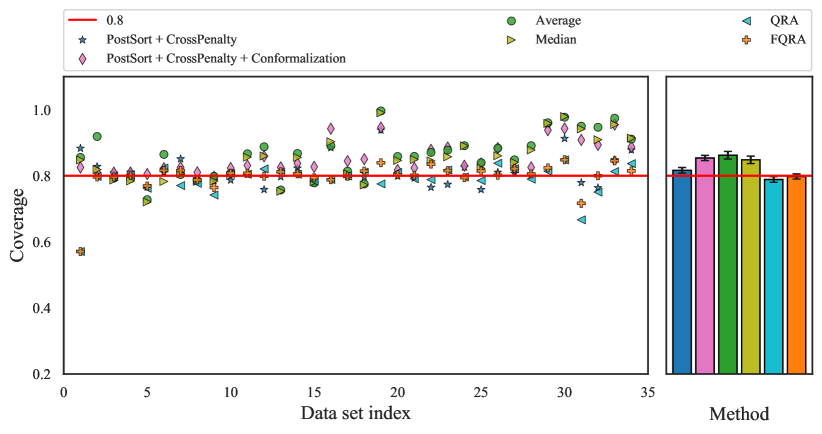
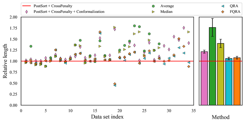
Figure 10: Comparing coverage of DQA, conformalized DQA, and other aggregators at the nominal 0.8 level. The display is as in Figure 7 (individual results per data set on left panel, averaged results on right panel). The key point is that conformalized DQA manages to achieve valid coverage on each individual data set.

Figure 11: Comparing prediction interval lengths from DQA, conformalized DQA, and others at the nominal 0.8 level. The display is again as in Figure 7 (individual results on the left, averaged results on the right). Conformalized DQA inflates interval lengths compared to DQA (in order to achieve valid coverage), but not by a huge amount, making it still clearly favorable to the Average and Median aggregators, and comparable to QRA.

7 Discussion

We studied methods for aggregating any number of conditional quantile models with multiple quantile levels, introducing weighted ensemble schemes with varying degrees of flexibility, and allowing for weight functions that vary over the input feature space. Being based on neural network architectures, our quantile aggregators are easy and efficient to implement in deep learning toolkits. To impose proper noncrossing of estimated quantiles, we examined penalties and isotonization operators that can be used either post hoc or during training. To guarantee proper coverage of central prediction intervals, we gave an efficient nested application of the conformal prediction method CQR-CV+ within our aggregation framework.

Finally, we carried out a large empirical comparison of all of our proposals and others from the literature across 34 data sets from two popular benchmark repositories, the most comprehensive evaluation quantile regression/aggregation methods that we know of. The conclusion is roughly that the most flexible model in our aggregation family, which we call DQA (deep quantile aggregation), combined with the simplest penalty and simplest post processor (just post sorting the quantile predictions), and conformalized using CQR-CV+, is often among the most accurate and well-calibrated aggregation methods available, and should be a useful method in the modern data scientist’s toolbox.

Appendix A Proofs

A.1 Proof of equivalence (6)

At the outset, we assume two conditions on $F$: it has a derivative $f$, and it yields an expectation. Starting with the right-hand side in (6), we can use substitute $Y=F^{-1}(\tau)$ to rewrite the integral as

$$2\int_{0}^{1}(1\{Y\leq F^{-1}(\tau)\}-\tau)(F^{-1}(\tau)-Y)\,\mathsf{d}\tau=2\int_{-\infty}^{\infty}(1\{Y\leq y\}-F(y))(y-Y)f(y)\,\mathsf{d}{y}.$$

Let $u^{\prime}(y)=2(1\{Y\leq y\}-F(y))f(y)$ and $v(y)=y-Y$. The idea is now to use integration by parts, but there are two subtleties. First, one has to be careful about framing the antiderivative $u$ of $u^{\prime}$, since $y\mapsto 1\{Y\leq y\}$ is not classically differentiable. Note that we can actually redefine $u^{\prime}$ to be

$$u^{\prime}(y)=2(1\{Y\leq y\}-F(y))(f(y)-\delta_{Y}(y)),$$

where $\delta_{Y}$ is the Dirac delta function centered at $Y$, because the “extra” piece integrates to zero:

$$\int_{-\infty}^{\infty}2(1\{Y\leq y\}-F(y))(y-Y)\delta_{Y}(y)\,\mathsf{d}{y}=2(1\{Y\leq y\}-F(y))(y-Y)\Big{|}_{y=Y}=0.$$

With this new definition of $u^{\prime}$, its antiderivative is rigorously

$$u(y)=-(1\{Y\leq y\}-F(y))^{2},$$

because, in the distributional sense, the derivative of the heavyside function $y\mapsto 1\{Y\leq y\}$ is indeed the delta function $\delta_{Y}$. Thus we have

$$\int_{-\infty}^{\infty}u^{\prime}(y)v(y)\,\mathsf{d}{y} =u(y)v(y)\Big{|}_{-\infty}^{\infty}-\int_{-\infty}^{\infty}u(y)v^{\prime}(y)\,\mathsf{d}{y}$$

$$=-(1\{Y\leq y\}-F(y))^{2}(y-Y)\Big{|}_{-\infty}^{\infty}+\int_{-\infty}^{\infty}(1\{Y\leq y\}-F(y))^{2}\,\mathsf{d}{y}.$$

The second subtlety is to show that the first term above is indeed zero. This is really a question of how fast the tails of $F$ decay. As $F$ yields an expectation, note that we must have $1-F(y)\lesssim y^{-p}$ for $p>1$ (since $1/y$ is not integrable on any one-sided interval $[q,\infty)$ for $q>0$). Hence

$$(1-F(y))y\lesssim y^{-p+1}\to 1\quad\text{as $y\to\infty$},$$

and the other limit, as $y\to-\infty$, is similar.

A.2 Proof of equivalence (8)

Starting with the right-hand side in (8), consider the two summands corresponding to $\tau\in\{\alpha/2,1-\alpha/2\}$:

$$2\psi_{\alpha/2}(Y-\ell_{\alpha})+2\psi_{\alpha/2}(Y-u_{\alpha}),$$ (30)

where we have used $\ell_{\alpha}=F^{-1}(\alpha/2)$ and $u_{\alpha}=F^{-1}(1-\alpha/2)$. If $Y>u_{\alpha}$, then (30) is

$$\alpha(Y-\ell_{\alpha})+2(1-\alpha/2)(Y-u_{\alpha})=\alpha(u_{\alpha}-\ell_{\alpha})+2(Y-u_{\alpha}).$$

Meanwhile, if $Y<\ell_{\alpha}$, then (30) is

$$2(1-\alpha/2)(\ell_{\alpha}-Y)+\alpha(u_{\alpha}-Y)=\alpha(u_{\alpha}-\ell_{\alpha})+2(\ell_{\alpha}-Y).$$

Lastly, if $Y\in[\ell_{\alpha},u_{\alpha}]$, then (30) is

$$\alpha(Y-\ell_{\alpha})+\alpha(u_{\alpha}-Y)=\alpha(u_{\alpha}-\ell_{\alpha}).$$

In each case, it matches the summand in the left-hand side of (8) corresponding to exclusion probability $\alpha$, which completes this proof.

A.3 Proof of Proposition 2

In this proof we denote the pinball loss, for a vector of quantiles $q\in\mathbb{R}^{m}$ across quantiles levels $\tau_{1},\ldots,\tau_{m}$, by

$$L(q,y)=\sum_{i=1}^{m}\psi_{\tau_{i}}(y-q_{i}).$$

A.3.1 Proof of part (i)

Suppose that there are only two quantile levels $\tau_{1}<\tau_{2}$, and abbreviate $q_{i}=\hat{g}(x;\tau_{i})$ for $i=1,2$. We will prove in this special case that sorting can only improve the pinball loss. Importantly, this suffices to prove the result in the general case as well, since sorting can always be achieved by a sequence of pairwise swaps (via bubble sort).

Assume $q_{1}>q_{2}$, otherwise there is nothing to prove. Denote the pinball loss by

$$L(q,y)=\psi_{\tau_{1}}(y-q_{1})+\psi_{\tau_{2}}(y-q_{2}).$$

We now break the argument down into three cases. In each case, when we speak of the loss difference, we mean the pre-sort minus the post-sort pinball loss (first line minus second line in each display that follows).

Case 1: $y>q_{1}$. Denoting $a=y-q_{1}$ and $b=y-q_{2}$ (and noting $b\geq a$), we have

$$L((q_{1},q_{2}),y) =\tau_{1}a+\tau_{2}b,$$

$$L((q_{2},q_{1}),y) =\tau_{1}b+\tau_{2}a,$$

so the loss difference is $(\tau_{2}-\tau_{1})(b-a)\geq 0$. I

Case 2: $y\in[q_{2},q_{1}]$. Denoting $a=q_{1}-y$ and $b=y-q_{2}$, we have

$$L((q_{1},q_{2}),y) =(1-\tau_{1})a+\tau_{2}b,$$

$$L((q_{2},q_{1}),y) =\tau_{1}b+(1-\tau_{2})a,$$

so the loss difference is $(\tau_{2}-\tau_{1})(a+b)\geq 0$.

Case 3: $y<q_{2}$. Denoting $a=q_{1}-y$ and $b=q_{2}-y$ (and noting $a\geq b$), we have

$$L((q_{1},q_{2}),y) =(1-\tau_{1})a+(1-\tau_{2})b,$$

$$L((q_{2},q_{1}),y) =(1-\tau_{1})b+(1-\tau_{2})a,$$

so the loss difference is $(\tau_{2}-\tau_{1})(a-b)\geq 0$. This completes the proof.

A.3.2 Proof of part (ii)

As in the proof of part (i), we will prove the result in a special case, and argue that it suffices to prove the result in general. Given $k+\ell$ quantile levels $\tau_{1}<\cdots<\tau_{k+\ell}$, we abbreviate $q_{i}=\hat{g}(x;\tau_{i})$ for $i=1,\ldots,k+\ell$. We suppose, in what follows, that $q_{1}=\cdots=q_{k}$ and $q_{k+1}=\cdots=q_{k+\ell}$. We then show that averaging can only improve the pinball loss, where by averaging, we mean replacing the original vector $(q_{1},\ldots,q_{k+\ell})$ by $(\bar{q},\ldots,\bar{q})$, with $\bar{q}=\frac{1}{k+\ell}\sum_{i=1}^{k+\ell}q_{i}$. This suffices to prove the desired result, because isotonic projection can be solved using PAVA, which carries out a sequence of steps (whenever there is a violation of the monotonicity condition) that are precisely of the form we study here.

Assume $q_{k}>q_{k+1}$, otherwise there is nothing to prove. We break the argument down into four cases. In each case, as in the proof of part (i), when we speak of the loss difference below, we mean the pre-sort loss minus the post-sort loss.

Case 1: $y\geq q_{k}$. We have

$$L((q_{1},\ldots,q_{k+\ell}),y) =\sum_{i=1}^{k}\tau_{i}(y-q_{k})+\sum_{i=k+1}^{k+\ell}\tau_{i}(y-q_{k+1}),$$

$$L((\bar{q},\ldots,\bar{q}),y) =\sum_{i=1}^{k+\ell}\tau_{i}(y-\bar{q}),$$

so the loss difference is

$$\sum_{i=1}^{k}\tau_{i}(\bar{q}-q_{k})+\sum_{i=k+1}^{k+\ell}\tau_{i}(\bar{q}-q_{k+1})=\frac{k\ell}{k+\ell}\bigg{(}\frac{1}{\ell}\sum_{i=k+1}^{k+\ell}\tau_{i}-\frac{1}{k}\sum_{i=1}^{k}\tau_{i}\bigg{)}(q_{k}-q_{k+1})\geq 0.$$

Case 2: $y\in[q_{k+1},q_{k}]$ and $y>\bar{q}$. We have

$$L((q_{1},\ldots,q_{k+\ell}),y) =\sum_{i=1}^{k}(1-\tau_{i})(q_{k}-y)+\sum_{i=k+1}^{k+\ell}\tau_{i}(y-q_{k+1}),$$

$$L((\bar{q},\ldots,\bar{q}),y) =\sum_{i=1}^{k+\ell}\tau_{i}(y-\bar{q}),$$

so the loss difference is

$$k(q_{k}-y)+\sum_{i=1}^{k}\tau_{i}(\bar{q}-q_{k})+\sum_{i=k+1}^{k+\ell}\tau_{i}(\bar{q}-q_{k+1})=k(q_{k}-y)+\frac{k\ell}{k+\ell}\bigg{(}\frac{1}{\ell}\sum_{i=k+1}^{k+\ell}\tau_{i}-\frac{1}{k}\sum_{i=1}^{k}\tau_{i}\bigg{)}(q_{k}-q_{k+1})\geq 0.$$

Case 3: $y\in[q_{k+1},q_{k}]$ and $y\leq\bar{q}$. We have

$$L((q_{1},\ldots,q_{k+\ell}),y) =\sum_{i=1}^{k}(1-\tau_{i})(q_{k}-y)+\sum_{i=k+1}^{k+\ell}\tau_{i}(y-q_{k+1}),$$

$$L((\bar{q},\ldots,\bar{q}),y) =\sum_{i=1}^{k+\ell}(1-\tau_{i})(\bar{q}-y),$$

so the loss difference is

$$\ell(y-q_{k+1})+\sum_{i=1}^{k}(1-\tau_{i})(q_{k}-\bar{q})+\sum_{i=k}^{k+\ell}(1-\tau_{i})(q_{k+1}-\bar{q})\\ =\ell(y-q_{k+1})+\frac{k\ell}{k+\ell}\bigg{(}\frac{1}{k}\sum_{i=1}^{k}(1-\tau_{i})-\frac{1}{\ell}\sum_{i={k+1}}^{k+\ell}(1-\tau_{i})\bigg{)}(q_{k}-q_{k+1})\geq 0.$$

Case 4: $y<q_{k}$. Then

$$L((q_{1},\ldots,q_{k+\ell}),y) =\sum_{i=1}^{k}(1-\tau_{i})(q_{k}-y)+\sum_{i=k+1}^{k+\ell}(1-\tau_{i})(q_{k+1}-y),$$

$$L((\bar{q},\ldots,\bar{q}),y) =\sum_{i=1}^{k+\ell}(1-\tau_{i})(\bar{q}-y),$$

so the loss difference is

$$\sum_{i=1}^{k}(1-\tau_{i})(q_{k}-\bar{q})+\sum_{i=k}^{k+\ell}(1-\tau_{i})(q_{k+1}-\bar{q})=\frac{k\ell}{k+\ell}\bigg{(}\frac{1}{k}\sum_{i=1}^{k}(1-\tau_{i})-\frac{1}{\ell}\sum_{i={k+1}}^{k+\ell}(1-\tau_{i})\bigg{)}(q_{k}-q_{k+1})\geq 0.$$

This completes the proof.

A.4 Proof of Proposition 5

A.4.1 Proof of part (i)

This is immediate from the fact that $f(v)=w_{1}f_{1}(v)+w_{2}f_{2}(v)$ and $f_{2}(v)/f_{1}(v)\to 0$.

A.4.2 Proof of part (ii)

This part is more subtle. Using (14), note that we may write

$$\frac{1}{\bar{f}(\bar{Q}(u))}=\frac{w_{1}}{f_{1}(Q_{1}(u))}+\frac{w_{2}}{f_{2}(Q_{2}(u))}.$$

For $v=\bar{Q}(u)$, consider

$$\frac{f_{1}(v)}{\bar{f}(v)}=\frac{w_{1}f_{1}(\bar{Q}(u))}{f_{1}(Q_{1}(u))}+\frac{w_{2}f_{1}(\bar{Q}(u))}{f_{2}(Q_{2}(u))}.$$

It will be convenient to work on the log scale. Introduce $p_{1}=\log f_{1}$ and $p_{2}=\log f_{2}$. Then it suffices to show that as $u\to 1$,

$$p_{1}(\bar{Q}(u))-p_{1}(Q_{1}(u))\to\infty,\quad\text{and}$$

$$p_{1}(\bar{Q}(u))-p_{2}(Q_{2}(u))\;\text{remains bounded away from $-\infty$},$$

or

$$p_{1}(\bar{Q}(u))-p_{2}(Q_{2}(u))\to\infty,\quad\text{and}$$

$$p_{1}(\bar{Q}(u))-p_{1}(Q_{1}(u))\;\text{remains bounded away from $-\infty$}.$$

We now divide the argument into two cases. Without a loss of generality, we set $w_{1}=w_{2}=1/2$.

Case 1: $p_{1}(Q_{1}(u))-p_{2}(Q_{2}(u))$ remains bounded away from $-\infty$. Denoting $v=\bar{Q}(u)$, $v_{1}=Q_{1}(u)$, $v_{2}=Q_{2}(u)$, we have, using log-concavity of $p_{1}$,

$$p_{1}(v)-p_{2}(v_{2}) =p_{1}(v_{1}/2+v_{2}/2)-p_{2}(v_{2})$$

$$\geq p_{1}(v_{1})/2+p_{1}(v_{2})/2-p_{2}(v_{2})$$

$$=\big{(}p_{1}(v_{1})-p_{2}(v_{2})\big{)}/2+\big{(}p_{1}(v_{2})-p_{2}(v_{2})\big{)}/2.$$

The first term above is bounded below by assumption; the second term diverges to $\infty$ (under our hypothesis that $f_{2}(v)/f_{1}(v)\to 0$).

Case 2: $p_{1}(Q_{1}(u))-p_{2}(Q_{2}(u))\to-\infty$. We have, just as in the first case,

$$p_{1}(v)-p_{1}(v_{1}) =p_{1}(v_{1}/2+v_{2}/2)-p_{1}(v_{1})$$

$$\geq p_{1}(v_{1})/2+p_{1}(v_{2})/2-p_{2}(v_{2})+p_{2}(v_{2})-p_{1}(v_{1})$$

$$=-\big{(}p_{1}(v_{1})-p_{2}(v_{2})\big{)}/2+\big{(}p_{1}(v_{2})-p_{2}(v_{2})\big{)}/2.$$

Now both terms above diverge to $\infty$, and this completes the proof.

Appendix B More experimental details and results

In the following, we provide further details about models: the hyperparameter space, optimization details, etc. In our experiments, for each method described below, we perform hyperparameter tuning over a randomly chosen subset of 20 values from the full Cartesian product of possibilities.

B.1 Base models

We consider $p=6$ base models in total. The first 3 are neural network models, that each compute quantile estimates differently. Each use a standard feed-forward (multilayer perceptron) architecture.

• Conditional Gaussian network (CGN, Lakshminarayanan et al., 2017): this model assumes that the conditional distribution of $Y|X=x$ is Gaussian. It therefore outputs estimates of sufficient statistics, namely the conditional mean $\mu(x)$ and variance $\sigma^{2}(x)$. It is optimized by minimizing the negative log-likelihood, and subsequent quantile estimation is done based on the normal distribution.

• Simultaneous quantile regression (SQR, Tagasovska and Lopez-Paz, 2019): this model takes as input a target quantile level $\tau$ concatenated with a feature vector $x$, and outputs a corresponding quantile estimate. It is trained by minimizing a pinball loss for many different randomly sampled quantile levels $\tau$. To estimate multiple quantile levels with SQR, we must thus feed in the same $x$ numerous times, each paired with a different quantile level $\tau$.

• Deep quantile regression (DQR): this model falls naturally out of our neural aggregation framework, as explained in Section 3.3. It is the only neural network based model considered in this paper that can easily utilize different isotonization approaches discussed in Section 4. For DQR as a base model in all experiments, we use the simplest method for ensuring noncrossing among the all options: the crossing penalty along with post sorting.

We optimize each of these neural network models using Adam (Kingma and Ba, 2015), and using ELU activation function (Clevert et al., 2016). We adaptively vary the mini-batch size depending on the data set size. They also share the same architecture/optimization hyperparameter search space: # of fully connected layers: {2, 3}, # of hidden units: {64, 128}, dropout ratio: {0.0, 0.05, 0.1}, learning rate: {1e-3, 3e-4}, weight decay: {1e-5, 1e-7}. In all settings, we use early stopping where the validation loss is evaluated every epoch and if it has not decreased for the last 500 updates, the optimization is stopped by returning the epoch with the lowest validation loss.

The next 3 base models are not neural networks.

• Quantile random forest (RandomForest, Meinshausen, 2006) and extremely randomized trees (ExtraTrees, Geurts et al., 2006): both models are based on random forests trained as regular (conditional mean) regressors. After training, quantile estimates are computed via empirical quantiles of the data in relevant leaf nodes of the trees.

• Quantile gradient boosting (LightGBM, Ke et al., 2017): this model is a gradient boosting framework that uses tree-based base learners. As a boosting framework, it can optimize the pinball loss, and thus be directly used for quantile regression. It handles multiple quantile levels by simply using a separate model for each level.

For the random forests models, we use the scikit-garden (https://scikit-garden.github.io/) implementation for both, and both have the same hyperparameter search space: minimum # of samples for splitting nodes: {8, 16, 64}, minimum # of sample for leaf nodes: {8, 16, 64} .

For the gradient boosting model, the hyperparameter space is: # of leaves: {10, 50, 100}, minimum child samples: {3, 9, 15}, minimum child weight: {1e-2, 1e-1, 1}, subsample ratio: {0.4, 0.6, 0.8}, subsample ratio of columns: {0.4, 0.6}, $\ell_{1}$ regularization weight: {1e-1, 1, 5}, $\ell_{2}$ regularization weight: {1e-1, 1, 5}.

B.2 Aggregation models

We consider 4 aggregation models from outside framework: Average, Median, quantile regression averaging (QRA, Nowotarski and Weron, 2015), and factor QRA (FQRA, Maciejowska et al., 2016). The first 3 do not require tuning. For FQRA, we tune over the number of factors, between 1-6 (the number of base models).

We also study a total of 6 aggregation models within our framework: three global aggregators and three local ones (each having coarse, medium, or fine weight parameterizations). For the global aggregators, the hyperparameter search space we use is: crossing penalty weight $\lambda$: {0.5, 1.0, 2.0, 5.0, 10.0}, crossing penalty margin scaling $\delta_{0}$: {1e-1, 5e-2, 1e-2, 1e-3, 1e-4}. For the local aggregators, the hyperparameter search space additionally includes: # of layers: {2, 3}, # of hidden units: {64, 128}, dropout ratio: {0.0, 0.05, 0.1}. All are optimized using the Adam optimizer (Kingma and Ba, 2015), ELU activation function (Clevert et al., 2016), and adaptively-varied mini-batch size. We also employ the same early stopping strategy as described above.

B.3 Revisiting Figure 1

Figure 12 plots the same results in Figure 1 but it displays a difference in WIS values, rather than a ratio of WIS values (which is how we define relative WIS). That is, shown on the y-axis is the difference of the WIS of each quantile regression minus that of DQA, where now 0 indicates equal WIS performance to DQA, and a number greater than 0 indicates worse performance than DQA. In general, WIS will be on the scale of the response variable, but recall that we have standardized the response variable in each data set, thus the comparison in Figure 12 makes sense across data sets. The story in this figure is very much similar to that in Figure 1, except that we can more clearly see that for some data sets with low PVE values (e.g., at index 5), there are a handful of models that perform a little better than DQA.

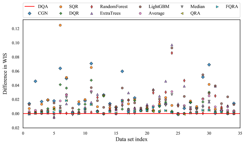
Figure 12: As in Figure 1, but with WIS differences (of each method to DQA) on the y-axis rather than WIS ratios.

References

- Ali et al. (2016) Alnur Ali, J Zico Kolter, and Ryan J Tibshirani. The multiple quantile graphical model. In Advances in Neural Information Processing Systems, 2016.
- Bahdanau et al. (2015) Dzmitry Bahdanau, Kyung Hyun Cho, and Yoshua Bengio. Neural machine translation by jointly learning to align and translate. In Proceedings of the International Conference on Learning Representations, 2015.
- Barber et al. (2021a) Rina Foygel Barber, Emmanuel J Candès, Aaditya Ramdas, and Ryan J Tibshirani. The limits of distribution-free conditional predictive inference. Information and Inference, 10(2):455–482, 2021a.
- Barber et al. (2021b) Rina Foygel Barber, Emmanuel J Candès, Aaditya Ramdas, and Ryan J Tibshirani. Predictive inference with the jackknife+. Annals of Statistics, 49(1):486–507, 2021b.
- Barlow et al. (1972) Richard E Barlow, D J Bartholomew, J M Bremner, and H D Brunk. Statistical Inference Under Order Restrictions: The Theory and Application of Isotonic Regression. Wiley, 1972.
- Belloni and Chernozhukov (2011) Alexandre Belloni and Victor Chernozhukov. -penalized quantile regression in high-dimensional sparse models. Annals of Statistics, 39(1):82–130, 2011.
- Benidis et al. (2022) Konstantinos Benidis, Syama Sundar Rangapuram, Valentin Flunkert, Yuyang Wang, Danielle Maddix, Caner Turkmen, Jan Gasthaus, Michael Bohlke-Schneider, David Salinas, Lorenzo Stella, François-Xavier Aubet, Laurent Callot, and Tim Januschowski. Deep learning for time series forecasting: Tutorial and literature survey. ACM Comput. Surv., 55(6), 2022.
- Bondell et al. (2010) Howard D Bondell, Brian J Reich, and Huixia Wang. Noncrossing quantile regression curve estimation. Biometrika, 97(4):825–838, 2010.
- Bracher et al. (2021) Johannes Bracher, Evan L Ray, Tilmann Gneiting, and Nicholas G Reich. Evaluating epidemic forecasts in an interval format. PLOS Computational Biology, 17(2):1–15, 2021.
- Browell et al. (2020) Jethro Browell, Ciaran Gilbert, Rosemary Tawn, and Leo May. Quantile combination for the eem20 wind power forecasting competition. In Proceedings of the International Conference on the European Energy Market, 2020.
- Chernozhukov et al. (2010) Victor Chernozhukov, Iván Fernández-Val, and Alfred Galichon. Quantile and probability curves without crossing. Econometrica, 78(3):1093–1125, 2010.
- Clevert et al. (2016) Djork-Arné Clevert, Thomas Unterthiner, and Sepp Hochreiter. Fast and accurate deep network learning by exponential linear units (ELUs). In International Conference on Learning Representations, 2016.
- Cumings-Menon and Shin (2020) Ryan Cumings-Menon and Minchul Shin. Probability forecast combination via entropy regularized Wasserstein distance. Entropy, 22(9), 2020.
- Dabney et al. (2018) Will Dabney, Mark Rowland, Marc Bellemare, and Rémi Munos. Distributional reinforcement learning with quantile regression. In Proceedings of the AAAI Conference on Artificial Intelligence, 2018.
- Dette and Volgushev (2008) Holger Dette and Stanislav Volgushev. Non-crossing non-parametric estimates of quantile curves. Journal of the Royal Statistical Society: Series B, 70(3):609–627, 2008.
- Dietterich (2000) Thomas G Dietterich. Ensemble methods in machine learning. In International Workshop on Multiple Classifier Systems, 2000.
- Dua and Graff (2017) Dheeru Dua and Casey Graff. UCI machine learning repository, 2017. URL http://archive.ics.uci.edu/ml.
- Erickson et al. (2020) Nick Erickson, Jonas Mueller, Alexander Shirkov, Hang Zhang, Pedro Larroy, Mu Li, and Alexander J Smola. AutoGluon-Tabular: Robust and accurate AutoML for structured data. arXiv: 2003.06505, 2020.
- Fakoor et al. (2020) Rasool Fakoor, Jonas Mueller, Nick Erickson, Pratik Chaudhari, and Alexander J Smola. Fast, accurate, and simple models for tabular data via augmented distillation. In Advances in Neural Information Processing Systems, 2020.
- Fung et al. (2002) Glenn Fung, Olvi Mangasarian, and Jude Shavlik. Knowledge-based support vector machine classifiers. In Advances in Neural Information Processing Systems, 2002.
- Gaillard et al. (2016) Pierre Gaillard, Yannig Goude, and Raphaël Nedellec. Additive models and robust aggregation for GEFCom2014 probabilistic electric load and electricity price forecasting. International Journal of forecasting, 32(3):1038–1050, 2016.
- Genest (1992) Christian Genest. Vincentization revisited. Annals of Statistics, 20(2):1137–1142, 1992.
- Geurts et al. (2006) Pierre Geurts, Damien Ernst, and Louis Wehenkel. Extremely randomized trees. Machine Learning, 6:3–42, 2006.
- Gneiting and Katzfuss (2014) Tilmann Gneiting and Matthias Katzfuss. Probabilistic forecasting. Annual Review of Statistics and Its Application, 1:125–151, 2014.
- Gneiting and Raftery (2007) Tilmann Gneiting and Adrian E Raftery. Strictly proper scoring rules, prediction, and estimation. Journal of the American Statistical Association, 102(477):359–378, 2007.
- Gneiting and Ranjan (2013) Tilmann Gneiting and Roopesh Ranjan. Combining predictive distributions. Electronic Journal of Statistics, 7:1747–1782, 2013.
- Hald (1998) Anders Hald. A History of Mathematical Statistics from 1750 to 1930. Wiley, 1998.
- Hardy et al. (1934) Godfrey H Hardy, John E Littlewood, and George Pólya. Inequalities. Camrbridge, 1934.
- Hatalis et al. (2017) Kostas Hatalis, Alberto J Lamadrid, Katya Scheinberg, and Shalinee Kishore. Smooth pinball neural network for probabilistic forecasting of wind power. arXiv: 1710.01720, 2017.
- Jacobs et al. (1991) Robert A Jacobs, Michael I Jordan, Steven J Nowlan, and Geoffrey E Hinton. Adaptive mixtures of local experts. Neural Computation, 3(1):79–87, 1991.
- Jain et al. (2020) Siddhartha Jain, Ge Liu, Jonas Mueller, and David Gifford. Maximizing overall diversity for improved uncertainty estimates in deep ensembles. In Proceedings of the AAAI Conference on Artificial Intelligence, 2020.
- Kapetanios et al. (2015) George Kapetanios, James Mitchell, Simon Price, and Nicholas Fawcett. Generalised density forecast combinations. Journal of Econometrics, 188(1):150–165, 2015.
- Ke et al. (2017) Guolin Ke, Qi Meng, Thomas Finley, Taifeng Wang, Wei Chen, Weidong Ma, Qiwei Ye, and Tie-Yan Liu. LightGBM: A highly efficient gradient boosting decision tree. In Advances in Neural Information Processing Systems, 2017.
- Kingma and Ba (2015) Diederik P Kingma and Jimmy Ba. Adam: A method for stochastic optimization. In International Conference on Learning Representations, 2015.
- Kivaranovic et al. (2020) Danijel Kivaranovic, Kory D Johnson, and Hannes Leeb. Adaptive, distribution-free prediction intervals for deep networks. In Proceedings of the International Conference on Artificial Intelligence and Statistics, 2020.
- Koenker (2005) Roger Koenker. Quantile Regression. Cambridge University Press, 2005.
- Koenker (2011) Roger Koenker. Additive models for quantile regression: Model selection and confidence bandaids. Brazilian Journal of Probability and Statistics, 25(3):239–262, 2011.
- Koenker and Bassett (1978) Roger Koenker and Gilbert Bassett. Regression quantiles. Econometrica, 46(1):33–50, 1978.
- Koenker and Hallock (2001) Roger Koenker and Kevin F Hallock. Quantile regression. Journal of economic perspectives, 15(4):143–156, 2001.
- Kuczmarski (2000) Robert J Kuczmarski. CDC growth charts: United States. US Department of Health and Human Services, Centers for Disease Control and Prevention, 2000.
- Kuleshov et al. (2018) Volodymyr Kuleshov, Nathan Fenner, and Stefano Ermon. Accurate uncertainties for deep learning using calibrated regression. In International Conference on Machine Learning, 2018.
- Laio and Tamea (2007) Francesco Laio and Stefania Tamea. Verification tools for probabilistic forecasts of continuous hydrological variables. Hydrology and Earth System Sciences, 11:1267–1277, 2007.
- Lakshminarayanan et al. (2017) Balaji Lakshminarayanan, Alexander Pritzel, and Charles Blundell. Simple and scalable predictive uncertainty estimation using deep ensembles. In Advances in Neural Information Processing Systems, 2017.
- Le et al. (2006) Quoc V Le, Alex J Smola, and Thomas Gärtner. Simpler knowledge-based support vector machines. In Proceedings of the International Conference on Machine Learning, 2006.
- Lei and Wasserman (2014) Jing Lei and Larry Wasserman. Distribution-free prediction bands for non-parametric regression. Journal of the Royal Statistical Society: Series B, 76(1):71–96, 2014.
- Lei et al. (2018) Jing Lei, Max G’Sell, Alessandro Rinaldo, Ryan J Tibshirani, and Larry Wasserman. Distribution-free predictive inference for regression. Journal of the American Statistical Association, 113(523):1094–1111, 2018.
- Lichtendahl et al. (2013) Kenneth C Lichtendahl, Yael Grushka-Cockayne, and Robert L Winkler. Is it better to average probabilities or quantiles? Management Science, 59(7):1594–1611, 2013.
- Lima and Meng (2017) Luiz Renato Lima and Fanning Meng. Out-of-sample return predictability: A quantile combination approach. Journal of Applied Econometrics, 32(4):877–895, 2017.
- Maciejowska et al. (2016) Katarzyna Maciejowska, Jakub Nowotarski, and Rafał Weron. Probabilistic forecasting of electricity spot prices using factor quantile regression averaging. International Journal of Forecasting, 32(3):957–965, 2016.
- Matheson and Winkler (1976) James E Matheson and Robert L Winkler. Scoring rules for continuous probability distributions. Management Science, 22(10):1087–1096, 1976.
- Meinshausen (2006) Nicolai Meinshausen. Quantile regression forests. Journal of Machine Learning Research, 7(35):983–999, 2006.
- Mukhoti et al. (2018) Jishnu Mukhoti, Pontus Stenetorp, and Yarin Gal. On the importance of strong baselines in Bayesian deep learning. In Advances in Neural Information Processing Systems, 2018.
- Nowotarski and Weron (2015) Jakub Nowotarski and Rafał Weron. Computing electricity spot price prediction intervals using quantile regression and forecast averaging. Computational Statistics, 30(3):791–803, 2015.
- Nowotarski and Weron (2018) Jakub Nowotarski and Rafał Weron. Recent advances in electricity price forecasting: A review of probabilistic forecasting. Renewable and Sustainable Energy Reviews, 81:1548–1568, 2018.
- Raftery et al. (2005) Adrian E Raftery, Tilmann Gneiting, Fadoua Balabdaoui, and Michael Polakowski. Using bayesian model averaging to calibrate forecast ensembles. Monthly Weather Review, 133(5):1155–1174, 2005.
- Ranjan and Gneiting (2010) Roopesh Ranjan and Tilmann Gneiting. Combining probability forecasts. Journal of the Royal Statistical Society: Series B, 72(1):71–91, 2010.
- Rasp and Lerch (2018) Stephan Rasp and Sebastian Lerch. Neural networks for postprocessing ensemble weather forecasts. Monthly Weather Review, 146(11):3885–3900, 2018.
- Ratcliff (1979) Roger Ratcliff. Group reaction time distributions and an analysis of distribution statistics. Psychological Bulletin, 86(3):446–461, 1979.
- Robertson et al. (1998) Tim Robertson, F T Wright, and Richard L Dykstra. Order Restricted Statistical Inference. Wiley, 1998.
- Romano et al. (2019) Yaniv Romano, Evan Patterson, and Emmanuel J Candès. Conformalized quantile regression. In Advances in Neural Information Processing Systems, 2019.
- Smyl and Hua (2019) Slawek Smyl and N Grace Hua. Machine learning methods for GEFCom2017 probabilistic load forecasting. International Journal of Forecasting, 35(4):1424–1431, 2019.
- Song et al. (2019) Hao Song, Tom Diethe, Meelis Kull, and Peter Flach. Distribution calibration for regression. In International Conference on Machine Learning, 2019.
- Stone (1961) Mervyn Stone. The opinion pool. Annals of Mathematical Statistics, 32(4):1339–1342, 1961.
- Tagasovska and Lopez-Paz (2019) Natasa Tagasovska and David Lopez-Paz. Single-model uncertainties for deep learning. In Advances in Neural Information Processing Systems, 2019.
- Takeuchi et al. (2006) Ichiro Takeuchi, Quoc V Le, Timothy D Sears, and Alexander J Smola. Nonparametric quantile estimation. Journal of Machine Learning Research, 7:1231–1264, 2006.
- Thomas and Ross (1980) Ewart A Thomas and Brian H Ross. On appropriate procedures for combining probability within the same family. Journal of Mathematical Psychology, 21:136–152, 1980.
- Tibshirani (2020) Ryan J Tibshirani. quantgen: Tools for generalized quantile modeling, 2020. URL https://github.com/ryantibs/quantgen.
- Timmermann (2006) Allan Timmermann. Forecast combinations. Handbook of Economic Forecasting, 1:135–196, 2006.
- Uniejewski and Weron (2021) Bartosz Uniejewski and Rafał Weron. Regularized quantile regression averaging for probabilistic electricity price forecasting. Energy Economics, 95(C):S0140988321000268, 2021.
- Van der Laan et al. (2007) Mark J Van der Laan, Eric C Polley, and Alan E Hubbard. Super learner. Statistical Applications in Genetics and Molecular Biology, 6(1), 2007.
- Vanschoren et al. (2013) Joaquin Vanschoren, Jan N van Rijn, Bernd Bischl, and Luis Torgo. OpenML: Networked science in machine learning. SIGKDD Explorations, 15(2):49–60, 2013.
- Vincent (1912) Stella Burnham Vincent. The function of the vibrissae in the behavior of the white rat. Behavior Monographs, 1(5), 1912.
- Vovk (2012) Vladimir Vovk. Conditional validity of inductive conformal predictors. Asian Conference on Machine Learning, 2012.
- Vovk et al. (2005) Vladimir Vovk, Alex Gammerman, and Glenn Shafer. Algorithmic Learning in a Random World. Springer, 2005.
- Vovk et al. (2018) Vladimir Vovk, Ilia Nouretdinov, Valery Manokhin, and Alex Gammerman. Cross-conformal predictive distributions. In Conformal and Probabilistic Prediction and Applications, 2018.
- Winkler (1972) Robert L Winkler. A decision-theoretic approach to interval estimation. Journal of the American Statistical Association, 67(337):187–191, 1972.
- Wolpert (1992) David Wolpert. Stacked generalization. Neural Networks, 5(2):241–259, 1992.
- Xie and Wen (2019) Zongxia Xie and Hao Wen. Composite quantile regression long short-term memory network. In International Conference on Artificial Neural Networks, 2019.
- Zhang et al. (2020) Shu Zhang, Yi Wang, Yutian Zhang, Dan Wang, and Ning Zhang. Load probability density forecasting by transforming and combining quantile forecasts. Applied Energy, 277:115600, 2020.