Topological Uhlmann phase transitions for a spin-$j$ particle in a magnetic field

Abstract

The generalization of the geometric phase to the realm of mixed states is known as Uhlmann phase. Recently, applications of this concept to the field of topological insulators have been made and an experimental observation of a characteristic critical temperature at which the topological Uhlmann phase disappears has also been reported. Surprisingly, to our knowledge, the Uhlmann phase of such a paradigmatic system as the spin-$j$ particle in presence of a slowly rotating magnetic field has not been reported to date. Here we study the case of such a system in a thermal ensemble. We find that the Uhlmann phase is given by the argument of a complex valued second kind Chebyshev polynomial of order $2j$. Correspondingly, the Uhlmann phase displays $2j$ singularities, occurying at the roots of such polynomials which define critical temperatures at which the system undergoes topological order transitions. Appealing to the argument principle of complex analysis each topological order is characterized by a winding number, which happen to be $2j$ for the ground state and decrease by unity each time increasing temperature passes through a critical value. We hope this study encourages experimental verification of this phenomenon of thermal control of topological properties, as has already been done for the spin-$1/2$ particle.

UhlmannJ dmorachisgalindo February 2021

I Introduction

The emergence of the geometric phase in quantum physics has been a groundbreaking eventBerry (1984). It has served as a tool to comprehend its fundamentals, as the spin statistics theoremBerry and Robbins (1997) or the Aharanov-Bohm effectBerry (1984). In the field of condensed matter physics the geometric phase is a quantity that comes out in the theoretical description of the quantum Hall effectNiu et al. (1985); Niu and Thouless (1984), the correct expression for the velocity of Bloch electronsBohm et al. (2003), ferromagnetismKing-Smith and Vanderbilt (1993); Xiao et al. (2010), topological insulatorsHasan and Kane (2010), among other phenomena. It is also a central concept in holonomic quantum computationSjöqvist, E. (2015).

Firstly proposed for adiabatic cyclic evolutionBerry (1984), the geometric phase concept has already been broadened to arbitrary evolution of a quantum stateAharonov and Anandan (1987); Mukunda and Simon (1993a, b) and is thus ubiquitous in quantum systems. Nevertheless, this approach to the geometric phase considers pure states only, while a more realistic description of quantum phenomena requires making use of the density matrix formalism.

The appropriate extension of the geometric phase to mixed states was developed by UhlmannUhlmann (1986, 1989) and is thus called the Uhlmann phase. It has been theoretically studied in the context of $1D$ and $2D$ topological insulatorsViyuela et al. (2014a); Rivas et al. (2013); Viyuela et al. (2015); He et al. (2018), for example the 1D SSH modelSu et al. (1979) and the Qi-Wu-Zhang 2D Chern insulator Qi et al. (2006). A key feature of these systems is the appearance of a critical temperatures above which the Uhlmann phase vanishes regardless of the topological character of the system in the ground state. This temperature sets a regime of stability of the topological properties in such systems, and has already been experimentally observed in a superconducting qubitRivas et al. (2018), which gives the Uhlmann phase a higher ontological status. Recently, a connection between a topological invariant (the Uhlmann number) and measurable physical quantities, like the dynamical conductivity was established through the linear response theoryLeonforte et al. (2019).

For pure quantum systems, a paradigmatic example to illustrate the abstract notions of quantum holonomies is the spin-$j$ particle interacting with a slowly rotating magnetic field. In its original paper, BerryBerry (1984) obtained the beautiful solid angle formula for the eigenstates of this system . More recently, a generalization of the solid angle formula for arbitrary spin-$j$ states has been found in terms of the state’s Majorana constellationLiu and Fu (2014); Majorana (1932) which also gives insight on their entanglement propertiesLiu and Fu (2016). From a more practical standpoint, the study of the geometric phase for a spin-$1/2$ is the workhorse to build 1-qubit holonomic quantum gatesSjöqvist, E. (2015); Sjöqvist et al. (2016), with a possible extension to $SU(2)$ qudit gates for higher spinsRandall et al. (2018). This makes the study of the geometric phase for spin-$j$ particles of vital importance.

Surprisingly, the problem of the Uhlmann phase of a spin-$j$ particle, even the $1/2$ case whose Hamiltonian models any two-level quantum system, has not been addressed yet, to our knowledge. Here, we calculated the Uhlmann phase of a spin-$j$ particle subjected to a slowly rotating magnetic field. We derived a compact analytical expression in terms of the argument of the complex valued second kind Chebyshev polynomialsArfken and Weber (2005); Gradshteyn and Rhyzik (2007) $U_{2j}(z)$ multiplied by the Pauli sign $(-1)^{2j}$. When the field describe a circle instead of a cone, the Uhlmann phase becomes topological with respect to temperature: the change from zero to $\pi$ (or viceversa) at certain critical temperatures related to the roots of $U_{2j}(z)$. Based on a theorem of complex analysis,Wegert, E. (2012); Needham (1998) we define the Chern-like Uhlmann numbersViyuela et al. (2014b) as winding numbers. For arbitrary direction of the external field, and as a function of temperature, the colored plot of the phase allows to identify visually the number of critical temperatures and the Uhlmann topological numbers for a given spin number $j$.

The paper is organized as follows. In section 2 we derive the Uhlmann phase for the spin-$j$ particle. In section 3 we show the emergence of multiple thermal topological transitions and obtain their corresponding Chern-like numbers numbers. In section 4 we analyse the Uhlmann phase with respect to temperature and magnetic field’s polar angle. Section 5 contains the conclusions.

II Uhlmann phase for an arbitrary spin $\boldsymbol{J}$ in an external magnetic field

The Uhlmann phase of a mixed quantum state is given by the expressionViyuela et al. (2015); He et al. (2018)

$$\Phi_{U} =\arg\left(\operatorname{Tr}\left[\hat{\rho}\,\mathcal{P}e^{\oint\hat{A}_{U}}\right]\right),$$ (1)

where $\hat{\rho}$ is the system’s density matrix with a spectral decomposition $\sum_{k}p_{k}\ket{k}\bra{k}$ and $\mathcal{P}$ is the path-ordering operatorBohm et al. (2003). The Uhlmann connection $\hat{A}_{U}$ is given by He et al. (2018)

$$\hat{A}_{U} =\sum\limits_{l,k}\frac{(\sqrt{p_{l}}-\sqrt{p_{k}})^{2}}{p_{l}+p_{k}}\bra{l}(d\ket{k})\ket{l}\bra{k},$$ (2)

where $d$ is the exterior derivative operatorBohm et al. (2003). This equation is written in the density matrix eigenbasis, thus a parameter dependence on the eigenkets is to be understood.

The Hamiltonian of a spin-$j$ particle interacting with a magnetic field is expressed

$$\hat{H} =B\mathbf{\hat{n}}\cdot\boldsymbol{{\hat{J}}},$$ (3)

where all physical constants which give raise to the interaction are taken into account in $B$. The vector operator $\boldsymbol{\hat{J}}$ has the components $(\hat{J}_{x},\hat{J}_{y},\hat{J}_{z})$, where $\hat{J}_{i}$ are the usual angular momentum matrices of spin $j$Sakurai and Napolitano (1994). We will consider the familiar fixed magnitude magnetic field that rotates along the $\mathbf{\hat{z}}$ axis at constant frequency. The unit vector $\mathbf{\hat{n}}=(\sin\theta\cos\phi,\sin\theta\sin\phi,\cos\theta)$ is taken with fixed $\theta$, while $\phi$ changes during the evolution from $0$ to $2\pi$. For a thermal ensemble, the corresponding density matrix is written as

$$\hat{\rho} =\frac{e^{-\beta B\mathbf{\hat{n}}\cdot\boldsymbol{\hat{J}}}}{Z}$$ (4)

where $\beta=1/k_{B}T$. The partition function $Z$ can be ignored in the calculation of the Uhlmann phase (1), since it is real and represents just a scaling factor of the complex number $\operatorname{Tr}[\hat{M}]$, where $\hat{M}=\hat{\rho}\,\mathcal{P}\operatorname{e}^{\oint\hat{A}_{U}}$. The thermal basis in this case is given by a rotated $\ket{j,m}$ basis, which, in Euler angle representation is given by

$$\ket{j,m;\mathbf{\hat{n}}} =e^{-i\phi\hat{J}_{z}}e^{-i\theta\hat{J}_{y}}e^{i\phi\hat{J}_{z}}\ket{j,m}\ .$$ (5)

The thermal occupation probabilities $p_{m}$ are readily seen to be $e^{-\beta Bm}/Z$.

We now proceed to calculate the the Uhlmann connection for the problem at hand. The factor involving the thermal occupation probabilities in (2) can be expressed as

$$\frac{(\sqrt{p_{m}}-\sqrt{p_{m^{\prime}}})^{2}}{p_{m}+p_{m^{\prime}}} =1-\operatorname{sech}[\beta B(m-m^{\prime})/2],$$ (6)

while the factor involving the exterior derivative $d$ becomes

$$\bra{m^{\prime}}d\ket{m}=ie^{-i(m^{\prime}-m)\phi}\sin\theta\bra{m^{\prime}}\hat{J}_{x}\ket{m},$$ (7)

plus a negligible diagonal term. Inserting equation (6) and (7) into (2) straightforwardly yields

$$\hat{A}_{U} =-i\eta\left(\hat{J}_{z}\sin\theta-e^{-i\phi\hat{J}_{z}}\hat{J}_{x}e^{i\phi\hat{J}_{z}}\cos\theta\right)d\phi,$$ (8)

where $\eta=\sin\theta[1-\operatorname{sech}(\beta B/2)]$. Calculation of the time ordered integral $\mathcal{P}\operatorname{e}^{\oint\hat{A}_{U}}$ is equivalent to solve a Schrödinger equation

$$i\frac{d}{d\phi}\hat{U} =\hat{V}(\phi)\hat{U},$$ (9)

where the solution $\hat{U}$ is the is just the time ordered exponential and $\hat{V}(\phi)$ is $i\hat{A}_{U}$. Solving eq.(9) for a closed loop followed by the direction of the external field results inBohm et al. (2003)

$$\mathcal{P}\operatorname{e}^{\oint\hat{A}_{U}} =(-1)^{2j}e^{-i2\pi[(\eta\sin\theta-1)\hat{J}_{z}-\eta\cos\theta\hat{J}_{x}]}.$$ (10)

In order to obtain the Uhlmann phase, we need to take the trace of $\hat{M}$. Except for the lowest total angular momentum representations, its exact closed form of is very cumbersome. Also we would need to find the specific matrix $\hat{M}$ for every $j$, which is not very practical for our purposes. A way out of this pothole is noticing that the object we need to trace out belongs to the Lie group $SL(2,\mathbb{C})$ in the $(j,0)$ representation. Basic representation theory of this groupN. Jeevanjee (2015) tells us that once the eigenvalues $(\lambda_{+},\lambda_{-})$ of the $(1/2,0)$ representation are known, the eigenvalues for higher $j$ are given by

$$\lambda^{2j}, \lambda^{2j-2},\dots,\lambda^{-2j+2},\lambda^{-2j}$$ (11)

with $\lambda=\lambda_{+}=\lambda^{-1}_{-}$, where $\lambda_{\pm}$ are the eingenvalues obtained from $j=1/2$. The equality above follows from the property that the group has unit determinant. Having noted this, the trace of $\hat{M}$ is readily seen to be

$$\operatorname{Tr}\left[\hat{\rho}\,\mathcal{P}e^{\oint\hat{A}_{U}}\right] =\frac{\lambda^{2j+1}-\lambda^{-2j-1}}{\lambda-\lambda^{-1}}.$$ (12)

The calculation that remains is to obtain the exact form of the eigenvalue $\lambda$. Diagonalization of $\hat{M}$ in the $(1/2,0)$ representation yields

$$\lambda= z+\sqrt{z^{2}-1},$$ (13)

with $z(\theta)$ being the complex variable

$$z =\cosh(\beta B/2)\cos(\pi C)-i\sinh(\beta B/2)\sin(\pi C)\frac{\cos\theta}{C}$$ (14)

where $C(\theta)=\sqrt{1-\sin^{2}\theta\tanh^{2}(\beta B/2)}$. The function $z(\theta)$ defines a simple closed curve in the complex plane, this property being of fundamental importance in what follows. With all these ingredients the Uhlmann phase is readily obtained:

$$\Phi_{U}^{(j)} =\arg\left[(-1)^{2j}\frac{(z+\sqrt{z^{2}-1})^{2j+1}-(z-\sqrt{z^{2}-1})^{2j+1}}{2\sqrt{z^{2}-1}}\right]$$

$$=\arg[(-1)^{2j}U_{2j}(z)],$$ (15)

where $U_{2j}(z)$ are the second kind Chebyshev polynomialsGradshteyn and Rhyzik (2007); we will refer to them just as Chebyshev polynomials to simplify matters. Equation (II) is valid under cyclic adiabatic evolution and is exact in this regime. The upper index $(j)$ tells us that the Uhlmann phase is that of a spin-$j$ particle. Also, in the low temperature limit this equation reduces to the corresponding Berry phaseBerry (1984); Bohm et al. (2003); Viyuela et al. (2015). We note that the nice compact form of result (II) is not simply a phase portrait of the Chebyshev polinomials in the whole complex plane, because the point $z(\theta)$ lies in a curve, with its shape depending on the parameter $\beta B$. It is interesting, however, the relation between the phase of polynomials $U_{2j}(z)$ and an observable phase of a quantum system. Appearance of Chebyshev polynomials in the Uhlmann phase can be traced back to $\hat{H}$ pertaining to $\mathfrak{su}(2)$ algebra and the particle being in thermal equilibrium. This generates an element of $SL(2,\mathbb{C})$ via $\hat{\rho}\operatorname{e}^{\oint\hat{A}_{U}}$, whose eigenvalues can always be written as $v\pm\sqrt{v^{2}-1}$, $v\in\mathbb{C}$. It would be interesting to explore what kind of mathematical object the Uhlmann phase would be when considering a Hamiltonian that belongs to $\mathfrak{su}(n)$ for $n>2$.

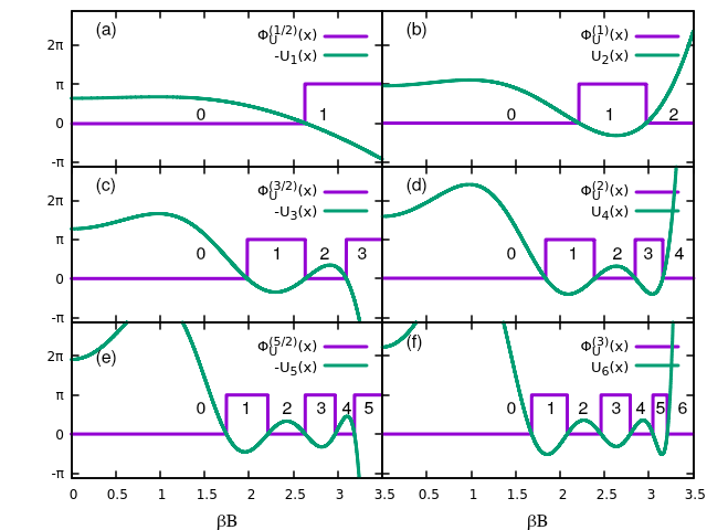
Figure 1: Uhlmann topological phases $\Phi^{(j)}_{U}$ and Chebyschev polynomials $(-1)^{2j}U_{2j}$ as functions of $\beta B$, for $\theta=\pi/2$. The left column presents the phase for the half integer values $j=1/2,3/2,5/2$ ((a),(c), and (e), respectively). The right column displays the phase for the integer values $j=1,2,3$ ((b), (d), and (f)). The integers between the zeros of the polynomials indicate associated winding numbers, corresponding to Uhlmann numbers $n_{U}^{(j)}$ (see text in Sec. IIIB).

III Topological Uhlmann phase transitions

III.1 Critical temperatures

The Uhlmann phase just obtained is determined by the argument of the complex Chebyshev polynomials $U_{2j}(z)$. The function $U_{2j}$ have real roots only, $2j$ in number, lying in the open interval $(-1,1)$Gradshteyn and Rhyzik (2007). The zeros of any polynomial $P_{n}(z)$ define points in the complex plane where its magnitude becomes zero, implying that its argument becomes undefinedWegert, E. (2012). These points are referred to as phase singularities and are a general phenomenon of wave physics. In the field of optics,Dennis et al. (2009) for example, they allow to define optical vortices which have found a number of applications.

The Uhlmann phase displays $2j$ phase singularities. The restriction on the variable $z(\theta)$ to acquire real values implies that $\theta=\pi/2$, that is, the magnetic field should lie on the equator of the sphere of directions. As a consequence, there are as many as $2j$ critical temperatures $T^{(j)}_{c,k}$ ($k=1,\ldots,2j$) determined by

$$\cosh(\beta_{k}B/2)\cos[\pi\operatorname{sech}(\beta_{k}B/2)]=\cos\left(\frac{k\pi}{2j+1}\right),$$ (16)

where on the right hand side is the $k$-th root of the Chebyshev polynomial $U_{2j}(x)$, with $x=z(\theta=\pi/2)$.

Figure 1 shows the Uhlmann phase as a function of $\beta B$ for $\theta=\pi/2$ and several values of $j$. Note that for half integer $j$ there is a negative sign multiplying $U_{2j}(x)$. It can be seen that $\Phi_{U}^{(j)}(\beta B)=\text{arg}[(-1)^{2j}U_{2j}(x)]$ is $0$ or $\pi$, and in this manner topological. The topological transitions, between trivial and nontrivial phases, occur at temperatures (or field magnitudes) such that the Chebyshev polynomials vanish, and the precise value, $0$ or $\pi$, of the phase $\Phi_{U}^{(j)}$ is determined by the sign of the polynomials times the Pauli sign $(-1)^{2j}$. Note that for very high temperatures ($\beta B\ll 1$) the Uhlmann phase vanishes, as expected for a system under thermal noiseViyuela et al. (2015). For very low temperatures ($\beta B\gg 1$), the phase $\Phi_{U}^{(j)}$ is either $\pi$ or zero for half integer and integer values of $j$, respectively. That is the expected behaviour because the Uhlmann phase of a thermal ensemble approaches the geometric phase of a pure system in its ground state as we approach zero temperatureViyuela et al. (2015). For example, a ground state spin-$j$ particle in a slowly rotating planar ($\theta=\pi/2$) magnetic field acquires a Berry phaseBerry (1984) $\gamma_{-j}=2\pi j$, consistent with the aforementioned. What is remarkable about this result is the emergence of many critical temperatures, distributed in a nonuniform way as $j$ varies. There are $2j$ critical temperatures, some of which are at higher or lower values from that of the $j=1/2$ case. Thus, additional nontrivial topological phases appear at higher temperatures in comparison to the simplest spin one-half particle, and are in this sense more robust against thermal noise. On the other hand, the critical temperatures cannot reach arbitrary large values for high $j$, given the constraint imposed by eq.(16), or equivalently, due to the fact that all the roots of $U_{2j}(z)$ lie in the interval $(-1,1)$.Gradshteyn and Rhyzik (2007)

Viyuela et al. predictViyuela et al. (2014b) the existence of two critical temperatures in a 2D topological insulator with high Chern numbers, suggesting the possibility of purely thermal topological transitions. Furthermore, the thermal topological phase transition for $j=1/2$ has already been confirmed experimentallyRivas et al. (2018) in a superconducting qubit. We regard this as a strong suggestion of the physical existence of multiple Uhlmann topological transitions for a spin-$j$ particle, and thus hope our results encourage experimental verification of this phenomenon.

III.2 Topological Uhlmann numbers

The case $j=1/2$ is illustrative. There is only one topological transition, occurring at $\beta B=2\ln(2+\sqrt{3})$ (Fig. 1(a)). Viyuela et al.Viyuela et al. (2014a)report this single critical temperature for three representative 1D models of topological insulators and superconductors. At zero temperature, $T=0$, the ground state of the system acquires a Berry phase of $\pi$ and a Chern number of $+1$. At finite temperature, for $T<T^{(1/2)}_{c,1}$ the same phase is preserved, but above the critical temperature the Uhlmann topological phase becomes trivial. This is in sharp contrast to the zero temperature behavior. A question that naturally arises at this point is about the invariants associated with the topological phases that occur for higher $j$. A look at Fig. 2 will give insight about writing the proper definition of them. The figure depicts the $z(\theta)$ curve (14) for four temperatures, where the dots mark the roots of $U_{3}(z(\theta))$. The smallest curve (purple) corresponds to the higher temperature while the largest (red) is for the lowest temperature. As the temperature decreases, the curve expands and progressively encloses the roots of $U_{3}$, whenever the temperature crosses a critical value $T^{(j)}_{c,k}$. The number of enclosed roots is zero at high temperatures, and ends up being $2j$ for low enough temperatures. This relates a topological property of $z(\theta)$, the number of roots enclosed, and the critical temperatures.

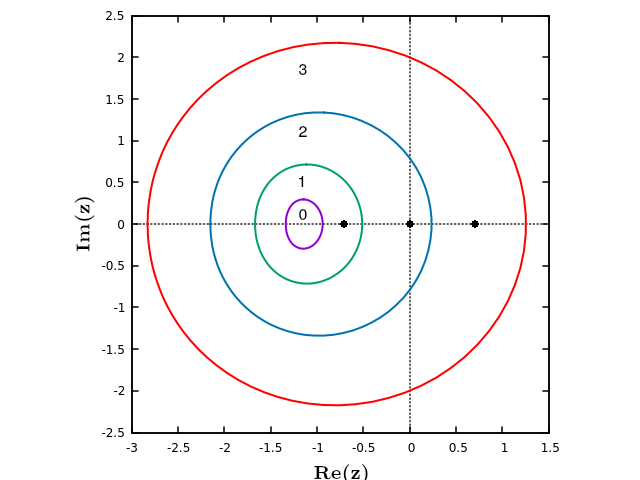
Figure 2: Argand diagram of $z(\theta)$ for several values of $\beta B$. Considering the case $j=3/2$, the points marked on the real axis are the roots of polynomial $U_{3}(z)$. At high enough temperatures the curve $z(\theta)$ (purple) does not enclose a single root. As temperature reduces the curve expands and encloses progressively the roots. The Uhlmann numbers are given by the number of roots inside $z(\theta)$.

According to the argument principle of complex analysisNeedham (1998); Wegert, E. (2012), if $z(\theta)$ encloses $k$ roots of $U_{2j}$, then the curve $U_{2j}(z(\theta))$ winds around the origin $k$ times, so the number of closed roots equals the winding number. The winding number of the curve $(-1)^{2j}U_{2j}(z(\theta))$ tells us how many times its phase changes from $0$ to $2\pi$,do Carmo (2016) but this phase is just $\Phi^{(j)}_{U}(\theta)$. This suggests the definition of Uhlmann numbers

$$n^{(j)}_{U}(T) =\frac{1}{2\pi}\int^{\pi}_{0}\frac{d\Phi^{(j)}_{U}(z(\theta))}{d\theta}d\theta,$$ (17)

to be the winding numbers of the $(-1)^{2j}U_{2j}(z(\theta))$ curve, for a temperature between two succesive critical values. These integer numbers are the equivalent of the Chern numbers of pure states.Xiao et al. (2010) In fact, expression (17) is consistent to that proposed as definition of Uhlmann numbers for two-dimensional topological insulatorsViyuela et al. (2015). Here, we have followed a more ad hoc path, motivated by the specific form of the Uhlmann phase (II), given in terms of polynomials.

Figure 3 shows the Uhlmann numbers for different values of $j$. The steps at which $n_{U}$ change by unity are located at the critical temperatures $T^{(j)}_{c,k}$. Note that the maximum value that $n_{U}$ takes on is $2j$, which equals the Chern number of a spin-$j$ particle in its ground stateBohm et al. (2003). The figure illustrates how the appearance of multiple critical temperatures makes possible transitions between nontrivial topological orders of the type $2j\to 2j-1\to 2j-2\to\ldots\to 0$ for increasing temperature.

In the model of a 2D topological insulator which presents two critical temperaturesViyuela et al. (2014b), there are three topological phases, one trivial with $n_{U}=0$ and two nontrivial with $n_{U}=1$ and 2, which can be accessed by varying the temperature. The appearance of $2j+1$ distinct Uhlmann numbers in the spin-$j$ particle is a more dramatic example of a system with more than one nontrivial order.

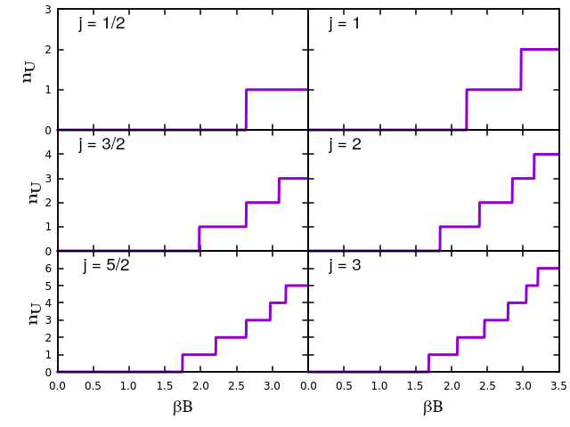
Figure 3: Uhlmann numbers $n_{U}$ as a function of temperature, for some values of the spin number $j$. The steps are located at a set of values of $\beta_{k}B$ which define critical temperatures $T^{(j)}_{c,k}$, with $k=1,\ldots,2j$.

IV Uhlmann geometric phases for arbitrary field direction

In Fig. 1 we show the temperature dependence of the Uhlmann phase for $\theta=\pi/2$. We now turn to analyse this dependence for directions in the whole interval $0\leq\theta\leq\pi$. Fig. 4 shows a color map of $\Phi^{(j)}_{U}(\theta,\beta B)$ for distinct spin number $j$. In each panel, $2j$ vortices can be distinguished along the line $\theta=\pi/2$, which correspond to the zeros of $U_{2j}(z)$, or equivalently, the critical temperatures. Note that for all cases the phase $\Phi^{(j)}_{U}(\theta,\beta B)\to 0$ for high temperatures $\beta B\ll 1$, as expected. On the other hand, for very low temperatures $\beta B\gg 1$, the Uhlmann phase must converge to the Berry phase,Berry (1984); Bohm et al. (2003) $\Phi^{(j)}_{U}(\theta,\beta B)\to 2j\pi(1-\cos\theta)$. For example, in the $j=1/2$ panel at low temperatures the sequence of colors as $\theta$ goes from zero to $\pi$ is that of the colorboxes on the right: the Uhlmann phase is $0$ for $\theta=0$ and increases up to $2\pi$ for $\theta=\pi$. Let us call that sequence of colors a phase cycle. For panels with higher $j$ at low temperatures we see that the phase cycles appear $2j$ times. Lowering temperature, the number of phase cycles decrease by unity when crossing a critical temperature. A look to the $j=1$ panel illustrates this point. For low temperatures, there are two phase cycles as $\theta$ goes from $0$ to $\pi$. When increasing temperature above the first critical value $T^{(1)}_{c,1}$ the Uhlmann phase only traverses one phase cycle, and none of them above the second critical temperature.

This behavior can also be illustrated in a similar way to that used to see the argument principle in action through the colored phase portrait of a complex function.Wegert, E. (2012) To take a concrete example, consider a simple closed path encircling the three singularities of the phase in Fig. 4 for $j=3/2$, and follow the number of phase cycles occurring when it is traversed. It can be seen that this number is exactly $2j$, the number of zeros enclosed, which is also the number of critical temperatures. The isochromatic lines (for instance the green ones) appear just $2j$ times. The number of cycles diminish by one each time the path shrinks to leave out a zero, where shrinks means to increase the temperature, in line with the geometrical interpretation of the Uhlmann numbers suggested by Fig. 2. Thus, in our problem the Uhlmann numbers can also be obtained from the number of cycles displayed by the function $\Phi^{(2j)}_{U}(\theta,\beta B)$ in the vicinity of singularities.

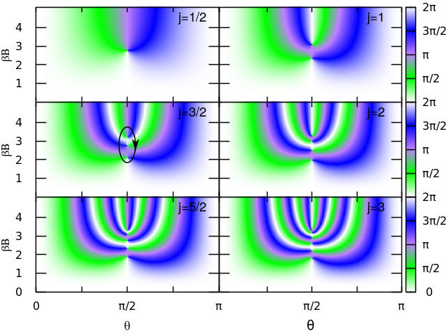
Figure 4: Uhlmann phases $\Phi^{(j)}_{U}(\theta,\beta B)$ for $j=1/2,1,\ldots,3$. There are $2j$ singularities along the $\theta=\pi/2$ line. The Uhlmann number characterizing a topological order can be obtained visually by encircling one or more singularities with a simple closed curve and counting the number of times an isochromatic line is repeated (see text).

V Conclusions

In this paper we have studied the Uhlmann phase of a spin-$j$ particle interacting with a slowly varying magnetic field. We obtained a simple expression for that phase given by the argument of complex valued second kind Chebyshev polynomials $U_{2j}(z)$ multiplied by the Pauli sign $(-1)^{2j}$, the complex variable $z$ being a function of the direction of the external field and temperature. As a consequence, $2j$ phase singularities appear which imply the possibility of topological phase transitions at $2j$ distinct critical temperatures. This is remarkably in contrast to the temperature dependence of the Uhlmann phase reported for topological insulators and superconductors. Based on the principle argument of complex analysis, we derived a proper topological invariant, the Uhlmann number, as a winding number associated to a topological order of the system, existing between two successive critical values of the temperature. The Uhlmann number lie between $0$ and $2j$.

Our study suggests a purely thermal manipulation of topological transitions of a spin-$j$ particle. This nontrivial effect has already been observed for the $j=1/2$ case and thus we hope this study encourages experimental verification of this phenomenon.

VI Acknowledgements

D.M.G. acknowledges support from Consejo Nacional de Ciencia y Tecnología (México). The authors thank Ernesto Cota and Jorge Villavicencio for fruitful discussions.

References

- Berry (1984) M. V. Berry, Proc. R. Soc. Lond. A 392 (1984), https://doi.org/10.1098/rspa.1984.0023.
- Berry and Robbins (1997) M. V. Berry and J. M. Robbins, Proc. R. Soc. Lond. A 453 (1997), 10.1098/rspa.1997.0096.
- Niu et al. (1985) Q. Niu, D. J. Thouless, and Y.-S. Wu, Phys. Rev. B 31, 3372 (1985).
- Niu and Thouless (1984) Q. Niu and D. J. Thouless, Journal of Physics A: Mathematical and General 17, 2453 (1984).
- Bohm et al. (2003) A. Bohm, Mostafazadeh, K. A., Q. H., Niu, and Zwanziger, The Geometric Phase in Quantum Systems (Springer-Verlag, 2003).
- King-Smith and Vanderbilt (1993) R. D. King-Smith and D. Vanderbilt, Phys. Rev. B 47, 1651 (1993).
- Xiao et al. (2010) D. Xiao, M.-C. Chang, and Q. Niu, Rev. Mod. Phys. 82, 1959 (2010).
- Hasan and Kane (2010) M. Z. Hasan and C. L. Kane, Rev. Mod. Phys. 82, 3045 (2010).
- Sjöqvist, E. (2015) Sjöqvist, E., Int. J. Quantum Chem. 115, 1311 (2015).
- Aharonov and Anandan (1987) Y. Aharonov and J. Anandan, Phys. Rev. Lett. 58, 1593 (1987).
- Mukunda and Simon (1993a) N. Mukunda and R. Simon, Ann. Phys. 228, 205 (1993a).
- Mukunda and Simon (1993b) N. Mukunda and R. Simon, Ann. Phys. 228, 269 (1993b).
- Uhlmann (1986) A. Uhlmann, Rep. Math. Phys. 24, 229 (1986).
- Uhlmann (1989) A. Uhlmann, Annalen der Physik 501, 63 (1989).
- Viyuela et al. (2014a) O. Viyuela, A. Rivas, and M. A. Martin-Delgado, Phys. Rev. Lett. 112, 130401 (2014a).
- Rivas et al. (2013) A. Rivas, O. Viyuela, and M. A. Martin-Delgado, Phys. Rev. B 88, 155141 (2013).
- Viyuela et al. (2015) O. Viyuela, A. Rivas, and M. A. Martin-Delgado, 2D Materials 2, 034006 (2015).
- He et al. (2018) Y. He, H. Guo, and C.-C. Chien, Phys. Rev. B 97, 235141 (2018).
- Su et al. (1979) W. P. Su, J. R. Schrieffer, and A. J. Heeger, Phys. Rev. Lett. 42, 1698 (1979).
- Qi et al. (2006) X.-L. Qi, Y.-S. Wu, and S.-C. Zhang, Phys. Rev. B 74, 045125 (2006).
- Rivas et al. (2018) A. Rivas, O. Viyuela, S. Gasparinetti, A. Wallraff, S. Filipp, and M. Martin-Delgado, npj Quantum Information 4 (2018), 10.1038/s41534-017-0056-9.
- Leonforte et al. (2019) L. Leonforte, D. Valenti, B. Spagnolo, and A. Carollo, Scientific Reports 9 (2019), 10.1038/s41598-019-45546-9.
- Liu and Fu (2014) H. D. Liu and L. B. Fu, Phys. Rev. Lett. 113, 240403 (2014).
- Majorana (1932) E. Majorana, Nuovo Cim 9, 43 (1932).
- Liu and Fu (2016) H. D. Liu and L. B. Fu, Phys. Rev. A 94, 022123 (2016).
- Sjöqvist et al. (2016) E. Sjöqvist, V. Azimi Mousolou, and C. M. Canali, Quantum Inf. Process. 15, 3995–4011 (2016).
- Randall et al. (2018) J. Randall, A. M. Lawrence, S. C. Webster, S. Weidt, N. V. Vitanov, and W. K. Hensinger, Phys. Rev. A 98, 043414 (2018).
- Arfken and Weber (2005) G. Arfken and H. Weber, Mathematical Methods for Physicists (Elsevier, 2005).
- Gradshteyn and Rhyzik (2007) I. Gradshteyn and I. Rhyzik, Table of Integrals, Series and Products. (Academic Press, 2007).
- Wegert, E. (2012) Wegert, E., Visual Complex Functions., 2nd ed. (Birkhäuser Basel, 2012).
- Needham (1998) T. Needham, Visual Complex Analysis (Clarendon Press, 1998).
- Viyuela et al. (2014b) O. Viyuela, A. Rivas, and M. A. Martin-Delgado, Phys. Rev. Lett. 113, 076408 (2014b).
- Sakurai and Napolitano (1994) J. Sakurai and J. Napolitano, Modern Quantum Mechanics (Addison-Wesley Publishing Company, 1994).
- N. Jeevanjee (2015) N. Jeevanjee, An Introduction to Tensors and Group Theory for Physicists., 2nd ed. (Birkhäuser, 2015).
- Dennis et al. (2009) M. R. Dennis, K. O’Holleran, and M. J. Padgett (Elsevier, 2009) pp. 293–363.
- Note (1) The extra factor of 2 arises from the definition used for .
- Note (2) If is a simple closed curve in the interval , so is .
- do Carmo (2016) M. do Carmo, Differential Geometry of Curves and Surfaces, 2nd ed. (Dover Publications, 2016).