An Optimal Deterministic Algorithm for Geodesic Farthest-Point Voronoi Diagrams in Simple Polygons

Abstract

Given a set $S$ of $m$ point sites in a simple polygon $P$ of $n$ vertices, we consider the problem of computing the geodesic farthest-point Voronoi diagram for $S$ in $P$. It is known that the problem has an $\Omega(n+m\log m)$ time lower bound. Previously, a randomized algorithm was proposed [Barba, SoCG 2019] that can solve the problem in $O(n+m\log m)$ expected time. The previous best deterministic algorithms solve the problem in $O(n\log\log n+m\log m)$ time [Oh, Barba, and Ahn, SoCG 2016] or in $O(n+m\log m+m\log^{2}n)$ time [Oh and Ahn, SoCG 2017]. In this paper, we present a deterministic algorithm of $O(n+m\log m)$ time, which is optimal. This answers an open question posed by Mitchell in the Handbook of Computational Geometry two decades ago.

1 Introduction

Let $P$ be a simple polygon of $n$ vertices in the plane. Let $S$ be a set of $m$ points, called sites, in $P$ (each site can be either in the interior or on the boundary of $P$). For any two points in $P$, their geodesic distance is the length of their Euclidean shortest path in $P$. We consider the problem of computing the geodesic farthest-point Voronoi diagram of $S$ in $P$, which is to partition $P$ into Voronoi cells such that all points in the same cell have the same farthest site in $S$ with respect to the geodesic distance.

This problem generalizes the Euclidean farthest Voronoi diagram of $m$ sites in the plane, which can be computed in $O(m\log m)$ time [23]; this is optimal as $\Omega(m\log m)$ is a lower bound. For the more general geodesic problem in $P$, Aronov et al. [3] showed that the complexity of the diagram is $\Theta(n+m)$ and provided an $O(n\log n+m\log m)$ time algorithm. The runtime is close to optimal as $\Omega(n+m\log m)$ is a lower bound. No progress had been made for over two decades until in SoCG 2016 Oh et al. [20] proposed an $O(n\log\log n+m\log m)$ time algorithm. Later in SoCG 2017 Oh and Ahn [19] gave another $O(n+m\log m+m\log^{2}n)$ time algorithm and in SoCG 2019 Barba [8] presented a randomized algorithm that can solve the problem in $O(n+m\log m)$ expected time.

In this paper, we give an $O(n+m\log m)$ time deterministic algorithm, which is optimal. The space complexity of the algorithm is $O(n+m)$. This answers an open question posed by Mitchell [17] in the Handbook of Computational Geometry two decades ago.

1.1 Related work

If all sites of $S$ are on the boundary of $P$, then better results exist. The algorithm of Oh et al. [20] can solve the problem in $O((n+m)\log\log n)$ time while the randomized algorithm of Barba [8] runs in $O(n+m)$ expected time.

The geodesic nearest-point Voronoi diagram for sites in a simple polygon has also attracted much attention. The problem also has an $\Omega(n+m\log m)$ time lower bound. The first close-to-optimal algorithm was given by Aronov [2] and the running time is $O((n+m)\log(n+m)\log n)$. Papadopoulou and Lee [21] improved the algorithm to $O((n+m)\log(n+m))$ time. Recent progress has been made by Oh and Ahn [19] who presented an $O(n+m\log m\log^{2}n)$ time algorithm and also by Liu [16] who designed an $O(n+m(\log m+\log^{2}n))$ time algorithm. Finally the problem was solved optimally in $O(n+m\log m)$ time by Oh [18].

Another closely related problem is to compute the geodesic center of a simple polygon $P$, which is a point in $P$ that minimizes the maximum geodesic distance from all points of $P$. Asano and Toussaint [4] first gave an $O(n^{4}\log n)$ time algorithm for the problem. Pollack et al. [22] derived an $O(n\log n)$ time algorithm. Recently the problem was solved optimally in $O(n)$ time by Ahn et al. [1]. The geodesic diameter of $P$ is the largest geodesic distance between any two points in $P$. Chazelle [9] first gave an $O(n^{2})$ time algorithm and then Suri [24] presented an improved $O(n\log n)$ time solution. Hershberger and Suri [13] finally solved the problem in $O(n)$ time.

All above results are for simple polygons. For polygons with holes, the problems become more difficult. The geodesic nearest-point Voronoi diagram for $m$ point sites in a polygon with holes of $n$ vertices can be solved in $O((n+m)\log(n+m))$ time by the algorithm of Hershberber and Suri [14]. Bae and Chwa [5] gave an algorithm for constructing the geodesic farthest-point Voronoi diagram and the algorithm runs in $O(nm\log^{2}(n+m)\log m)$ time. For computing the geodesic diameter in a polygon with holes, Bae et al. [6] solved the problem in $O(n^{7.73})$ or $O(n^{7}(h+\log n))$ time, where $h$ is the number of holes. For computing the geodesic center, Bae et al. [7] first gave an $O(n^{12+\epsilon})$ time algorithm, for any constant $\epsilon>0$; Wang [26] solved the problem in $O(n^{11}\log n)$ time.

1.2 Our approach

We follow the algorithm scheme in [19], which in turn follows that in [3]. Specifically, we first compute the geodesic convex hull of all sites of $S$ in $O(n+m\log m)$ time [11, 12, 25], and then compute the geodesic center $c^{*}$ of the hull in $O(n+m)$ time [1]. Aronov [3] showed that the farthest Voronoi diagram forms a tree with $c^{*}$ as the root and all leaves on $\partial P$, the boundary of $P$. We construct the farthest Voronoi diagram restricted to $\partial P$; this can be done in $O(n+m)$ time by a recent algorithm of Oh et al. [20] once the geodesic convex hull of $S$ is known.

Next we run a reverse geodesic sweeping algorithm to extend the diagram from $\partial P$ to the interior of $P$ (i.e., based on all leaves on $\partial P$ and the root $c^{*}$ of the tree, we want to construct the tree). Here we use a geodesic sweeping circle that consists of all points with the same geodesic distance from $c^{*}$. Aronov [3] implemented this sweeping algorithm in $O((n+m)\log(n+m))$ time. Oh and Ahn [19] gave an improved solution of $O(n+m\log m+m\log^{2}n)$ time by using a data structure for the following query problem: Given three points in $P$, compute the point that is equidistant from them. Oh and Ahn [19] built a data structure in $O(n)$ time that can answer each query in $O(\log^{2}n)$ time, and that is why the time complexity of their algorithm has a $\log^{2}n$ factor. We improve the query time to $O(\log n)$ (with $O(n)$ time preprocessing) with the help of the following observations. First, the three points involved in a query are three sites of $S$ whose Voronoi cells are adjacent along the sweeping circle. Second, among the three sites involved in a query, for every two sites whose Voronoi cells are adjacent, the sweeping algorithm provides us with a point equidistant to them. These observations along with the tentative prune-and-search technique of Kirkpatrick and Snoeyink [15] lead us to a query algorithm of $O(\log n)$ time. Consequently, the sweeping algorithm can be implemented in $O(n+m\log m)$ time.

We should point out that in her algorithm for computing the geodesic nearest-point Voronoi diagram, Oh [18] also announced an $O(\log n)$ time algorithm for the above query problem and her algorithm also uses the tentative prune-and-search technique (although the details are omitted due to the page limit). However, the difference is that she uses a balanced geodesic triangulation [10] and her result is based on the assumption that the sought point of the query lies in a known geodesic triangle $\triangle$ and the three query points are in the same subpolygon of $P$ separated by a side of $\triangle$ (see Lemma 4.2 in [18]). For our problem, we do not need the balanced geodesic triangulation and do not have such an assumption. Instead, our algorithm relies on the observations mentioned above.

The rest of the paper is organized as follows. Section 2 defines notation and introduces some concepts. The algorithm for constructing the geodesic Voronoi diagram is described in Section 3. Section 4 presents the algorithm for a lemma about the query problem discussed above.

2 Preliminaries

Like the previous work [3, 8, 20, 19], for ease of discussion, we make a general position assumption that no vertex of $P$ is equidistant from two sites of $S$ and no point of $P$ has four farthest sites. We occasionally use polygon vertex to refer to a vertex of $P$ and use polygon edge to refer to an edge of $P$.

For any two points $p$ and $q$ in $P$, let $\pi(p,q)$ denote the (Euclidean) shortest path from $p$ to $q$ in $P$; let $d(p,q)$ denote the length of $\pi(p,q)$. $\pi(p,q)$ is also called the geodesic path and $d(p,q)$ is called the geodesic distance between $p$ and $q$. The vertex of $\pi(p,q)$ adjacent to $q$ (resp., $p$) is called the anchor of $q$ (resp., $p$) in $\pi(p,q)$.

For any two points $a$ and $b$ in the plane, denote by $\overline{ab}$ the line segment with $a$ and $b$ as endpoints, and denote by $|\overline{ab}|$ the length of the segment.

For any two sites $s$ and $t$ of $S$, their bisector, denoted by $B(s,t)$, consists of all points of $P$ equidistant from them, i.e., $B(s,t)=\{p\ |\ d(s,p)=d(t,p),p\in P\}$. Due to the general position assumption, Aronov et al. [2] showed that $B(s,t)$ is a smooth curve connecting two points on $\partial P$ with no other points common with $\partial P$ and $B(s,t)$ comprises $O(n)$ straight and hyperbolic arcs (a straight arc is a line segment); the endpoints of the arcs are breakpoints, each of which is the intersection of $B(s,t)$ and a segment extended from a polygon vertex $u$ to another polygon vertex $v$ such that $u$ is an anchor of $v$ in $\pi(s,v)$ or in $\pi(t,v)$ (it is possible that $u=s$ or $u=t$); e.g., see Fig. 2.

For any site $s\in S$, define $C(s)$ as the region consisting of all points $p$ of $P$ whose farthest site is $s$, i.e., $C(s)=\{p\ |\ d(p,s)\geq d(p,s^{\prime}),s^{\prime}\in S\}$. We call $C(s)$ the (farthest) Voronoi cell of $s$. Note that $C(s)$ may be empty; if $C(s)$ is not empty, then it is simply connected [3]. The Voronoi cells of all sites of $S$ form a partition of $P$. We define the geodesic farthest-point Voronoi diagram (or farthest Voronoi diagram for short), denoted by $\mbox{$F\!V\!D$}(S)$, as the closure of the interior of $P$ minus the union of the interior of $C(s)$ for all $s\in S$; alternatively, $\mbox{$F\!V\!D$}(S)=\{p\in B(s,t)\ |\ s,t\in S\text{ and }d(s,p)=\max_{r\in S}d(r,p)\}$. A point $v$ of $\mbox{$F\!V\!D$}(S)$ is a Voronoi vertex if it is an intersection of a bisector with $\partial P$ or if it has degree $3$ (i.e., it has three equidistant sites). The curve of $\mbox{$F\!V\!D$}(S)$ connecting two adjacent vertices is called a Voronoi edge, which is a portion of a bisector of two sites. Note that a Voronoi edge may not be of constant size because it may contain multiple breakpoints. While $\mbox{$F\!V\!D$}(S)$ has $O(m)$ Voronoi vertices and edges, the total complexity of $\mbox{$F\!V\!D$}(S)$ is $O(n+m)$ [3].

A subset $P^{\prime}$ of $P$ is geodesically convex if $\pi(p,q)$ is in $P^{\prime}$ for any two points $p$ and $q$ in $P^{\prime}$. The geodesic convex hull of $S$ in $P$, denoted by $\mbox{$G\!C\!H$}(S)$, is the common intersection of all geodesically convex sets containing $S$. $\mbox{$G\!C\!H$}(S)$ is a weakly simple polygon of at most $n+m$ vertices. Let $c^{*}$ be the geodesic center of $\mbox{$G\!C\!H$}(S)$, which is also the geodesic center of $S$ [3]. Note that $c^{*}$ must be on a Voronoi edge of $\mbox{$F\!V\!D$}(S)$. Indeed, if $c^{*}$ has three farthest sites in $S$, then $c^{*}$ is a Voronoi vertex; otherwise it has two farthest sites and thus is in the interior of an edge of $\mbox{$F\!V\!D$}(S)$. Aronov [3] proved that $\mbox{$F\!V\!D$}(S)$ is a tree with $c^{*}$ as the root and all leaves on $\partial P$; he also showed that only sites on the boundary of $\mbox{$G\!C\!H$}(s)$ have nonempty cells in $\mbox{$F\!V\!D$}(S)$ and the ordering of the sites with nonempty cells around the boundary of $\mbox{$G\!C\!H$}(s)$ is the same as the ordering of their Voronoi cells around $\partial P$ (the ordering lemma). Note that a site on the boundary of $\mbox{$G\!C\!H$}(s)$ may still have an empty Voronoi cell and intuitively this is because $P$ is not large enough [3].

Consider any three points $s,t,r$ in $P$. The vertex farthest to $s$ in $\pi(s,t)\cap\pi(s,r)$ is called the junction vertex of $\pi(s,t)$ and $\pi(s,r)$. The closure of the interior of the geodesic convex hull $\mbox{$G\!C\!H$}(s,t,r)$ is called the geodesic triangle of $s$, $t$, and $r$, denoted by $\triangle(s,t,r)$, whose boundary is composed of three convex chains $\pi(s^{\prime},t^{\prime})$, $\pi(t^{\prime},r^{\prime})$, $\pi(r^{\prime},s^{\prime})$, where $s^{\prime}$ is the junction vertex of $\pi(s,t)$ and $\pi(s,r)$, and $t^{\prime}$ and $r^{\prime}$ are defined likewise; e.g., see Fig. 2. The three convex chains are called sides of $\triangle(s,t,r)$. The three vertices $s^{\prime}$, $t^{\prime}$, and $r^{\prime}$ are called the apexes of $\triangle(s,t,r)$.

Figure 1: Illustrating the bisector $B(s,t)$ (the dashed curve) with three breakpoints.

Figure 2: Illustrating a geodesic triangle $\triangle(s,t,r)$ (the gray region).

3 Computing the farthest Voronoi diagram $\mbox{$F\!V\!D$}(S)$

In this section, we present our algorithm for computing the farthest Voronoi diagram $\mbox{$F\!V\!D$}(S)$.

First, we compute the geodesic convex hull $\mbox{$G\!C\!H$}(S)$ of $S$ in $O(n+m\log m)$ time [11, 12, 25]. Second, we compute the geodesic center $c^{*}$ of $\mbox{$G\!C\!H$}(S)$ in $O(n+m)$ time [1]. Third, we compute the portion of $\mbox{$F\!V\!D$}(S)$ restricted to the polygon boundary $\partial P$, i.e., the leaves of $\mbox{$F\!V\!D$}(S)$. This can be done in $O(n+m)$ time by the algorithm in [20]. The fourth step is to extend the diagram to the interior of $P$, i.e., construct the tree $\mbox{$F\!V\!D$}(S)$ based on all its leaves and the root $c^{*}$. This is achieved by a reverse geodesic sweeping algorithm, whose details are described below.

The algorithm first computes the adjacency information of $\mbox{$F\!V\!D$}(S)$. Specifically, we will compute the locations of all Voronoi vertices of $\mbox{$F\!V\!D$}(S)$; for Voronoi edges, however, we will not compute them exactly (i.e., the locations of their breakpoints will not be computed) but only output their incident Voronoi vertices, i.e., if $u$ and $v$ are two Voronoi vertices incident to the same Voronoi edge, then we will output the pair $(u,v)$ as an abstract Voronoi edge. In this way, we will output the abstract tree $\mbox{$F\!V\!D$}(S)$ with the exact locations of all Voronoi vertices; this is called the topological structure of $\mbox{$F\!V\!D$}(S)$ in [19]. After having the topological structure, Oh and Ahn [19] gave an algorithm that can construct $\mbox{$F\!V\!D$}(S)$ in additional $O(n+m\log m)$ time. More specifically, with $O(n)$ time preprocessing, each Voronoi edge can be computed in $O(\log n+k)$ time, where $k$ is the number of breakpoints in the Voronoi edge (see Section 4 of [19] for details). As $\mbox{$F\!V\!D$}(S)$ has $O(m)$ Voronoi edges, the total time for computing all Voronoi edges is $O(m\log n+K)$, where $K$ is the total number of breakpoints on all Voronoi edges. As $K=O(n+m)$ [3], the total time is bounded by $O(n+m\log n)$, which is $O(n+m\log m)$. In the following, we will focus on computing the topological structure of $\mbox{$F\!V\!D$}(S)$.

We use a reverse geodesic sweeping as in [3, 19]. Roughly speaking, the sweep line is a geodesic circle $C$ consisting of all points in $P$ that have the same geodesic distance from the geodesic center $c^{*}$ of $S$. This statement is actually not quite accurate as initially the sweep circle is just the boundary of $P$. During the sweeping, we maintain the sites whose Voronoi cells currently intersect $C$; these sites are stored in a cyclic linked list $\mathcal{L}$ ordered by their intersections with $C$. Initially when $C=\partial P$, as we already have the leaves of $\mbox{$F\!V\!D$}(S)$, we can build $\mathcal{L}$ in $O(n+m)$ time. Note that $|\mathcal{L}|=O(m)$. During the algorithm, $C$ will shrink until $c^{*}$; an event happens when $C$ hits a Voronoi vertex, which will be computed on the fly. Specifically, for each triple of adjacent sites $s,t,r$ in the list $\mathcal{L}$, we compute the point, denoted by $\alpha(s,t,r)$, equidistant from them, which is the intersection of the bisectors $B(s,t)$ and $B(t,r)$. Due to our general position assumption, $\alpha(s,t,r)$ is unique if it exists (see Lemma 2.5.3 [3]). We store all these $\alpha$-points in a priority queue $Q$, ordered by decreasing geodesic distance from $c^{*}$. In order to compute the $\alpha$-points, for any pair of adjacent sites $s$ and $t$ in $\mathcal{L}$, we maintain a Voronoi vertex, denoted by $\beta(s,t)$, on their bisector $B(s,t)$ with the following property: $\beta(s,t)$ is outside or on the current geodesic circle $C$. Initially, we set $\beta(s,t)$ to be the Voronoi vertex on $\partial P$ incident to the Voronoi cells of $s$ and $t$; so the above property holds as $C=\partial P$.

The main loop of the algorithm works as follows. As long as $Q$ is not empty, we repeatedly extract the point with largest geodesic distance from $c^{*}$ and let the point be $\alpha(s,t,r)$ defined by three sites $s,t,r$ in this order in $\mathcal{L}$. We report $\alpha(s,t,r)$ as a Voronoi vertex and report $(\beta(s,t),\alpha(s,t,r))$ and $(\beta(t,r),\alpha(s,t,r))$ as two abstract Voronoi edges. We remove $t$ from $\mathcal{L}$ and set $\beta(s,r)=\alpha(s,t,r)$. Let $x$ be the neighbor of $s$ other than $r$ in $\mathcal{L}$ and let $y$ be the neighbor of $r$ other than $s$. We remove $\alpha(x,s,t)$ and $\alpha(t,r,y)$ from $Q$ if they exist. Next, we compute $\alpha(x,s,r)$ and $\alpha(s,r,y)$ (if exist) as well as their geodesic distances from $c^{*}$, and insert them into $Q$.

For the running time, there are $O(m)$ events, for the total number of Voronoi vertices of $\mbox{$F\!V\!D$}(S)$ is $O(m)$ [3], and thus the total time of the algorithm is $O(m\cdot\sigma)$, where $O(\sigma)$ is the time for computing each $\alpha$ point. Lemma 1, which will be proved later in Section 4, is for computing the $\alpha$-points.

Lemma 1

With $O(n)$ time preprocessing, for any triple of adjacent sites $s,t,r$ in $\mathcal{L}$ at any moment during the algorithm, given the two Voronoi vertices $\beta(s,t)$ and $\beta(t,r)$, our algorithm can do the following in $O(\log n)$ time: if $\alpha(s,t,r)$ is a Voronoi vertex, then compute it; otherwise, either compute $\alpha(s,t,r)$ or return null.

We remark that Lemma 1 is sufficient for the correctness of our geodesic sweeping algorithm as only Voronoi vertices are essential. If the algorithm returns null, the event will not be inserted to $Q$. With Lemma 1 at hand, our geodesic sweeping algorithm computes the topological structure of $\mbox{$F\!V\!D$}(S)$ in $O(n+m\log m)$ time. After that, as discussed above, we can compute the full diagram $\mbox{$F\!V\!D$}(S)$ in additional $O(n+m\log m)$ time by the techniques of Oh and Ahn [19]. Also, the space of the algorithm is bounded by $O(n+m)$.

Theorem 1

The geodesic farthest-point Voronoi diagram of a set of $m$ points in a simple polygon of $n$ vertices can be computed in $O(n+m\log m)$ time and $O(n+m)$ space.

4 Algorithm for Lemma 1

In this section, we present our algorithm for Lemma 1. We first present an algorithm in Section 4.1 for the following triple-point geodesic center query problem: given any three points in $P$, compute their geodesic center in $P$, which is a point that minimizes the largest geodesic distance from the three query points. Oh and Ahn [19] solved this problem in $O(\log^{2}n)$ time, after $O(n)$ time preprocessing. Our algorithm runs in $O(\log n)$ time also with $O(n)$ time preprocessing. This algorithm will be used as a subroutine in our algorithm for Lemma 1, which will be discussed in Section 4.2.

4.1 The triple-point geodesic center query problem

As preprocessing, we construct the two-point shortest path query data structure by Guibas and Hershberger [11, 12] and we refer to it as the GH data structure. The data structure can be constructed in $O(n)$ time, after which given any two points $p$ and $q$ in $P$, the geodesic distance $d(p,q)$ can be computed in $O(\log n)$ time and the geodesic path $\pi(p,q)$ can be output in additional time linear in the number of edges of $\pi(p,q)$.

Consider three query points $s$, $t$, and $r$ in $P$. Our goal is to compute their geodesic center, denoted by $c$. We follow the algorithm scheme in [19]. Consider the geodesic convex hull $\mbox{$G\!C\!H$}(s,t,r)$ and the geodesic triangle $\triangle(s,t,r)$. We know that $c$ is the geodesic center of $\mbox{$G\!C\!H$}(s,t,r)$ [3]. Depending on whether $c$ is in the interior of $\triangle(s,t,r)$, there are two cases.

4.1.1 $c$ is not in the interior of $\triangle(s,t,r)$

If $c$ is not in the interior of $\triangle(s,t,r)$, then it must be on the geodesic path of two points of $\{s,t,r\}$. Without loss of generality, we assume that $c\in\pi(s,t)$. Note that $c$ must be the middle point of $\pi(s,t)$. To locate $c$ in $\pi(s,t)$, we wish to do binary search on the vertices of $\pi(s,t)$. It was claimed in [19] that the query algorithm of the GH data structure returns $\pi(s,t)$ as a binary tree (so that binary search can be done in a straightforward way), in particular, when the simpler approach in [12] is utilized. In fact, this is not quite correct. Indeed, the binary tree structures in both [11] and [12] are used for representing convex chains (or more rigorously, semiconvex chains [12]). However, $\pi(s,t)$ is actually a string [11], which in general is not a semiconvex chain. The data structure for representing a string is a tree but not a binary tree because a node in the tree may have three children.

Here for completeness, we provide a general binary search scheme on the geodesic path $\pi(p,q)$ returned by the GH data structure for any two query points $p$ and $q$ in $P$. Suppose we are looking for either a vertex or an edge of $\pi(p,q)$, denoted by $w^{*}$ in either case, and we have access to an oracle such that given any vertex $v\in\pi(p,q)$, the oracle can determine whether $w^{*}$ is in $\pi(p,v)$ or in $\pi(v,q)$. Then, we have the following lemma.

Lemma 2

With $O(n)$ time preprocessing, given any two query points $p$ and $q$, the sought vertex or edge $w^{*}$ can be located by a binary search algorithm that calls the oracle on $O(\log n)$ vertices of $\pi(p,q)$, and the total time of the binary search excluding the time for calling the oracle is $O(\log n)$. In particular, the middle point of $\pi(p,q)$ can be found in $O(\log n)$ time.

Proof: We will use notation and concepts from the GH data structure [11] without much explanation. To represent convex chains, we utilize the simper way given in [12], i.e., persistent binary trees with the path-copying method.

Consider the query points $p$ and $q$. The GH query algorithm combines $O(\log\log n)$ “small” hourglasses of size $O(\log n)$ and two “big” hourglasses of size $O(n)$ to assemble the path $\pi(p,q)$, which is represented as a string [11]. Combining two hourglasses involves computing a tangent between them such that the tangent belongs to $\pi(p,q)$. Thus, the algorithm will produce $O(\log\log n)$ tangents. For our problem, we explicitly consider these tangents and call the oracle on every vertex of these tangents. This calls the oracle $O(\log\log n)$ times. After that we can determine an hourglass that contains $w^{*}$. If it is a small hourglass, then since it has $O(\log n)$ vertices, we can simply call the oracle on every vertex to locate $w^{*}$. In the following, we assume that $w^{*}$ is in a big hourglass and let $\pi$ be the portion of $\pi(p,q)$ in the hourglass.

The endpoints of $\pi$ can be obtained during the GH query algorithm. $\pi$ from one end to the other consists of a convex chain, a string, and another convex chain in order. The two connection vertices between the string and the two convex chains can be maintained during the preprocessing. We call the oracle on these two vertices, after which we can determine the one of the three portions of $\pi$ that contains $w^{*}$. If it is a convex chain, then as a convex chain is represented by a binary tree of height $O(\log n)$ [12], we can apply binary search on this tree in a standard way; after calling the oracle on $O(\log n)$ vertices, $w^{*}$ can be obtained. In the following, we assume that the string of $\pi$ contains $w^{*}$. By slightly abusing notation, we still use $\pi$ to denote the string.

The string $\pi$ is represented by a tree $T$. However, each node of $T$ may have three children. Consider the root $v$ of $T$. In general, $\pi$ is a derived string and $v$ has three children: a left subtree $L$ representing a derived string, a middle subtree $M$ representing a fundamental string, and a right subtree $R$ representing another derived string. The fundamental string consists of two convex chains linked by a tangent edge and each derived string consists of two derived strings and a fundamental string in the middle. The height of $T$ is $O(\log n)$. The connecting vertex between the left string and the middle string and the connecting vertex between the middle string and the right string are maintained in the preprocessing and thus available during the query algorithm. We call the oracle on the two connecting vertices and then determine which string contains $w^{*}$. If the left or the right string contains $w^{*}$, then we proceed on the corresponding subtree of $v$ recursively. Otherwise, the middle string contains $w^{*}$. Again, the middle string consists of two convex chains linked by a tangent edge, which is available to us due to the preprocessing. We call the oracle on the two vertices of the tangent edge to determine which convex chain contains $w^{*}$ (or whether the tangent edge contains $w^{*}$). After that, since a convex chain is represented by a binary tree of height $O(\log n)$, we can finally locate $w^{*}$ by calling the oracle on $O(\log n)$ vertices using the binary tree. In this way, after $O(\log n)$ oracle calls, we can reach a fundament string and then $w^{*}$ can be finally located after another $O(\log n)$ oracle calls.

In summary, by calling the oracle on $O(\log n)$ vertices of $\pi(p,q)$, $w^{*}$ can be found.

To compute the middle point of $\pi(p,q)$, we first compute the geodesic distance $d(p,q)$ in $O(\log n)$ time by using the GH data structure. Then, we can follow the above binary search scheme and each time when the oracle is called on a vertex $v$, we also keep track of the geodesic distance $d(p,v)$ using the GH data structure. By comparing $d(p,v)$ with $d(p,q)/2$, we can decide which way to proceed the search. In this way, the middle point of $\pi(p,q)$ can be determined in $O(\log n)$ time. $\Box$

With Lemma 2 at hand, we can find $c$ on $\pi(s,t)$ in $O(\log n)$ time.

We can determine whether $c$ is in the interior of $\triangle(s,t,r)$ in $O(\log n)$ time using Lemma 2 as follows. First, we determine whether $c$ is the middle point of $\pi(s,t)$. To do so, we first compute the middle point $p_{st}$ of $\pi(s,t)$ by Lemma 2. Then, we compute $d(s,p_{st})$ and $d(r,p_{st})$ in $O(\log n)$ time using the GH data structure. It is not difficult to see that $p_{st}$ is $c$ if and only if $d(s,p_{st})\geq d(r,p_{st})$. If $p_{st}\neq c$, then we use the same way to determine whether the middle point of $\pi(s,r)$ (resp., $\pi(r,t)$) is $c$. If the above algorithm fails to locate $c$, then we know that $c$ is in the interior of $\triangle(s,t,r)$.

The above finds $c$ in $O(\log n)$ time for the case where $c$ is not in the interior of $\triangle(s,t,r)$.

4.1.2 $c$ is in the interior of $\triangle(s,t,r)$

We proceed to the case where $c$ is in the interior of $\triangle(s,t,r)$. Our algorithm utilizes the tentative prune-and-search technique of Kirkpatrick and Snoeyink [15].

First observe that in this case $c$ must be equidistant from all three points $s$, $t$, and $r$. Let $s^{\prime}$ be the junction vertex of $\pi(s,t)$ and $\pi(s,r)$. Define $t^{\prime}$ and $r^{\prime}$ similarly. With the GH data structure, each junction vertex can be computed in $O(\log n)$ time [11].

Define $p_{s}$, $p_{t}$, and $p_{r}$ to be the anchors of $c$ in $\pi(s,c)$, $\pi(t,c)$, and $\pi(r,c)$, respectively. Note that the segment connecting $c$ to $p_{s}$ (resp., $p_{t}$, $p_{r}$) is tangent to the side of $\triangle(s,t,r)$ that contains it. As $c$ is equidistant to $s$, $t$, and $r$, $c$ is the common intersection of the three bisectors $B(s,t)$, $B(s,r)$, and $B(t,r)$.

Observation 1

The middle point $p_{st}$ of $\pi(s,t)$ must be in $\pi(s^{\prime},t^{\prime})$; the middle point $p_{sr}$ of $\pi(s,r)$ must be in $\pi(s^{\prime},r^{\prime})$; the middle point $p_{tr}$ of $\pi(t,r)$ must be in $\pi(t^{\prime},r^{\prime})$.

Proof: We only prove the case for $p_{st}$ since the other two cases are similar. Assume to the contrary that $p_{st}\not\in\pi(s^{\prime},t^{\prime})$. Then, either $p_{st}\in\pi(s,s^{\prime})\setminus\{s^{\prime}\}$ or $p_{st}\in\pi(t,t^{\prime})\setminus\{t^{\prime}\}$. We assume it is the former case as the analysis for the latter case is similar. Then, $d(s,s^{\prime})>d(t,s^{\prime})$. Note that $d(s,c)=d(s,s^{\prime})+d(s^{\prime},c)$ as $c$ is in the interior of $\triangle(s,t,r)$. Hence, $d(s,c)>d(t,s^{\prime})+d(s^{\prime},c)\geq d(t,c)$. But this incurs contradiction as $c$ is equidistant from $s$ and $t$. $\Box$

Since $p_{s}$ is the anchor of $c$ in $\pi(s,c)$, $p_{s}$ has smaller geodesic distance from $s$ than from $t$ or $r$. Hence, by Observation 1, $p_{s}$ must be in $\gamma_{s}=\pi(s^{\prime},p_{st})\cup\pi(s^{\prime},p_{sr})$, which consists of two convex chains; we call $\gamma_{s}$ a pseudo-convex chain. Similarly, $p_{t}$ must be in $\gamma_{t}=\pi(t^{\prime},p_{st})\cup\pi(t^{\prime},p_{tr})$ and $p_{r}$ must be in $\gamma_{r}=\pi(r^{\prime},p_{tr})\cup\pi(r^{\prime},p_{sr})$. We consider $p_{st}$ and $p_{sr}$ as two ends of $\gamma_{s}$. If we move a point $p$ on $\gamma_{s}$ from one end to the other, then the slope of the tangent line of $\gamma_{s}$ at $p$ continuously changes. Further, $p_{s}$ is the only point on $\gamma_{s}$ such that $\overline{cp_{s}}$ is tangent to $\gamma_{s}$. Similar properties hold for $\gamma_{t}$, $p_{t}$, $\gamma_{r}$, and $p_{r}$.

With the above discussion, we are now in a position to describe our algorithm for computing $c$. First, we compute the three junction vertices and the three middle points $s^{\prime}$, $t^{\prime}$, $r^{\prime}$, $p_{st}$, $p_{sr}$, and $p_{tr}$. This can be done in $O(\log n)$ time using the GH data structure. To compute $c$ (as well as locate $p_{s}$, $p_{t}$, and $p_{r}$), we resort to the tentative prune-and-search technique [15], as follows.

To avoid the lengthy background explanation, we follow the notation in [15] without definition. We will rely on Theorem 3.9 in [15]. To this end, we need to define three continuous and monotone-decreasing functions $f$, $g$, and $h$. We define them in a way similar in spirit to Theorem 4.10 in [15] for finding a point equidistant to three convex polygons. Indeed, our problem may be considered as a weighted case of their problem because each point in our pseudo-convex chains has a weight that is equal to its geodesic distance from one of $s$, $t$, and $r$.

Figure 3: Illustrating the geodesic triangle $\triangle(s,t,r)$ and the definition of the function $f(a)$ for $a\in A=\gamma_{s}$.

We parameterize over $[0,1]$ each of the three pseudo-convex chains $A=\gamma_{s}$, $B=\gamma_{t}$, and $C=\gamma_{r}$ from one end to the other in counterclockwise order around $\triangle(s,t,r)$. For example, without loss of generality, we assume that $s^{\prime}$, $t^{\prime}$, and $r^{\prime}$ are counterclockwise around $\triangle(s,t,r)$. Then, $\gamma_{s}$ is parameterized from $p_{sr}$ to $p_{st}$ over $[0,1]$, i.e., each value of $[0,1]$ corresponds to a slope of a tangent at a point on $\gamma_{s}$. For each point $a$ of $A$, we define $f(a)$ to be the parameter of the point $b\in B$ such that the tangent of $A$ at $a$ and the tangent of $B$ at $b$ intersect at a point on the bisector $B(s,t)$ of $s$ and $t$ (e.g., see Fig. 3). Similarly, we define $g(b)$ for $b\in B$ with respect to $C$ and define $h(c)$ for $c\in C$ with respect to $A$. One can verify that all three functions are continuous and monotone-decreasing (the tangent at an apex of $\triangle(s,t,r)$ is not unique but the issue can be handled [15]). The fixed-point of the composition of the three functions $h\cdot g\cdot f$ corresponds to $c$, which can be computed by applying the tentative prune-and-search algorithm of Theorem 3.9 [15].

To see that the algorithm can be implemented in $O(\log n)$ time, we need to show that given any $a\in A$ and any $b\in B$, we can determine whether $f(a)>b$ in $O(1)$ time. To this end, we first find the intersection $p$ of the tangent of $A$ at $a$ and the tangent of $B$ at $b$. Then, $d(s,a)+|\overline{pa}|<d(t,b)+|\overline{pb}|$ if and only if $f(a)>b$. We will discuss below that the values $d(s,a)$ and $d(t,b)$ will be available during the tentative prune-and-search algorithm. Note that here the tangent of $A$ at $a$ actually refers to the half-line of the tangent whose concatenation with $\pi(s^{\prime},a)$ is still a convex chain (so that the shortest path can follow that half-line), as shown in Fig. 3. Hence, it is possible that the tangent half-line of $a$ does not intersect the tangent half-line of $b$. If that happens, either the tangent half-line of $a$ intersects the backward extension of the tangent half-line of $b$ or the backward extension of the tangent half-line of $a$ intersects the tangent half-line of $b$; in the former case we have $f(a)<b$ and in the latter case $f(a)>b$. Similar properties hold for functions of $g$ and $h$. Finally, we show that we have appropriate data structures to represent the three pseudo-convex chains $A$, $B$, and $C$ so that the algorithm can terminate in $O(\log n)$ rounds. We only discuss $A$ since other two are similar. When the algorithm picks the first vertex of $A$ to test, we will use the vertex $s^{\prime}$. After the test, the algorithm will proceed on $A$ on one side of $s^{\prime}$, say, on $\pi(s^{\prime},p_{st})$. We apply the binary search scheme of Lemma 2 on $\pi(s^{\prime},p_{st})$, which will test $O(\log n)$ vertices. Further, whenever a vertex $a\in\pi(s^{\prime},p_{st})$ is tested, the binary search scheme of Lemma 2 can keep track of $d(s,a)$. Therefore, applying the tentative prune-and-search technique in Theorem 3.9 [15] can compute the geodesic center $c$ in $O(\log n)$ time.

The following lemma summarizes our result on the triple-point geodesic center query problem.

Lemma 3

With $O(n)$ time preprocessing, the geodesic center of any three query points in $P$ can be computed in $O(\log n)$ time.

4.2 Proving Lemma 1

With Lemma 3, we are ready to present our algorithm for Lemma 1. Consider any three sites $s$, $t$, $r$ as specified in the statement of Lemma 1. Our goal is to compute the point $\alpha(s,t,r)$, which is equidistant from the three sites. Recall that we have two points $\beta(s,t)$ and $\beta(t,r)$ available for us, which are critical to the success of our approach.

The first step of our algorithm is to apply the algorithm for Lemma 3 to compute the geodesic center $c$ of the three sites. We check whether $c$ is equidistant to the three sites, in $O(\log n)$ time. If yes, $\alpha(s,t,r)=c$ and we are done. In the following we assume otherwise.

Our algorithm may not compute $\alpha(s,t,r)$ even if it exists, but will guarantee to do so if $\alpha(s,t,r)$ is a Voronoi vertex of $\mbox{$F\!V\!D$}(S)$. This is sufficient for constructing $\mbox{$F\!V\!D$}(S)$ correctly. Hence, in what follows we assume that $\alpha(s,t,r)$ is a Voronoi vertex. This implies that there are two Voronoi edges connecting $\alpha(s,t,r)$ with $\beta(s,t)$ and $\beta(t,r)$, respectively. Recall that $c^{*}$ is the geodesic center of $S$. The following observation was discovered by Aronov et al. [3].

Observation 2

(Aronov et al. [3]) If a point $p$ moves from $\beta(s,t)$ (resp., $\beta(t,r)$) to $\alpha(s,t,r)$ along the Voronoi edge, both $d(c^{*},p)$ and $d(t,p)$ are monotonically decreasing.

To simplify the notation, unless otherwise stated, we use $\alpha$ to refer to $\alpha(s,t,r)$. We define the three junction vertices $s^{\prime}$, $t^{\prime}$, and $r^{\prime}$ in the same way as before, which are the three apexes of the geodesic convex hull $\triangle(s,t,r)$. Without loss of generality, we assume that $s^{\prime}$, $t^{\prime}$, and $r^{\prime}$ are counterclockwise around the boundary of $\triangle(s,t,r)$ (e.g., see Fig. 2). We define $p_{s}$, $p_{t}$, and $p_{r}$ as the anchors of $\alpha$ in $\pi(s,\alpha)$, $\pi(t,\alpha)$, and $\pi(r,\alpha)$, respectively. Define $p_{st}$, $p_{sr}$, and $p_{tr}$ as the middle points of $\pi(s,t)$, $\pi(s,r)$, and $\pi(t,r)$, respectively.

The following observation, obtained from the results of Aronov [2], will occasionally be used later.

Observation 3

(Aronov [2]) Suppose $x$ and $y$ are two points of $P$ such that their bisector $B(x,y)$ does not contain any vertex of $P$. Then, for any point $z\in P$, the shortest path $\pi(x,z)$ (resp., $\pi(y,z)$) either does not intersect $B(x,y)$ or intersects it at a single point.

Proof: All arguments here are from Aronov [2]. $B(x,y)$ divides $P$ into two subpolygons; one of them, denoted by $P_{x}$, contains $x$ and the other, denoted by $P_{y}$, contains $y$. We assume that neither $P_{x}$ nor $P_{y}$ contains $B(x,y)$. All points in $P_{x}$ are closer to $x$ than to $y$ and all points in $P_{y}$ are closer to $y$ than to $x$. Let $z$ be any point in $P$. If $z\in P_{x}$, then $\pi(x,z)$ is in $P_{x}$. If $z\in B(x,y)$, then $\pi(x,z)\setminus\{z\}$ is in $P_{x}$ due to the general position assumption. If $z\in P_{y}$, then $\pi(x,z)$ intersects $B(x,y)$ at a single point. Similar results hold for $\pi(y,z)$. $\Box$

Recall that $\alpha(s,t,r)$ is not $c$. Hence, $c$ must be equidistant to two sites and the geodesic distance from them to $c$ is strictly larger than that from the third site to $c$. Depending on what the two sites are, there are three cases $d(c,s)=d(c,r)>d(c,t)$, $d(c,t)=d(c,r)>d(c,s)$, and $d(c,t)=d(c,s)>d(c,r)$. The following lemma shows that the latter two cases cannot happen.

Lemma 4

Neither $d(c,t)=d(c,r)>d(c,s)$ nor $d(c,t)=d(c,s)>d(c,r)$ can happen.

Proof: Note that the two cases are symmetric and thus we only discuss the case $d(c,t)=d(c,r)>d(c,s)$.

Assume to the contrary that $d(c,t)=d(c,r)>d(c,s)$ happens. Then, $c$ is the middle point of $\pi(t,r)$. Consider the farthest Voronoi diagram $\mbox{$F\!V\!D$}(s,t,r)$ with respect to the three sites $s,t,r$ only (without considering other sites of $S$). Then, $\alpha$ is a vertex of the diagram, i.e., the three Voronoi edges bounding the three cells of $s$, $t$, and $r$ meet at $\alpha$ (e.g., see Fig. 4). Since $d(c,t)=d(c,r)>d(c,s)$, $c$ is on the Voronoi edge $E(t,r)$ bounding the cells of $t$ and $r$. By the definition of $\beta(t,r)$, it is also on $E(t,r)$. Hence, all three points $\alpha$, $c$, and $\beta(t,r)$ are on $E(t,r)$. Let $E^{\prime}(t,r)$ be the portion of $E(t,r)$ between $\alpha$ and $\beta(t,r)$. Since both $\beta(t,r)$ and $\alpha$ are vertices of $\mbox{$F\!V\!D$}(S)$, $E^{\prime}(t,r)$ must be an edge of $\mbox{$F\!V\!D$}(S)$ bounding the two cells of $t$ and $r$. By Observation 2, if we move a point $p$ on $E^{\prime}(t,r)$ from $\beta(t,r)$ to $\alpha$, $d(t,p)$ is monotonically decreasing.

Figure 4: Illustrating the proof of Lemma 4. The three solid curves are the three Voronoi edges of $\mbox{$F\!V\!D$}(s,t,r)$. The dotted curve is the shortest path $\pi(r,t)$.

Since $c$ is the middle point of $\pi(t,r)$, if we move a point $p$ on the bisector $B(t,r)$ from one end to the other, $d(t,p)$ will first striclty decreases until $p=c$ and then strictly increases. Note that $E^{\prime}(t,r)\subseteq E(t,r)\subseteq B(t,r)$. Note also that $E^{\prime}(t,r)$ has $\alpha$ and $\beta(t,r)$ as its two endpoints. Depending on whether $E^{\prime}(t,r)$ contains $c$, there are two cases.

• If $E^{\prime}(t,r)$ does not contain $c$, then $c$, $\beta(t,r)$, and $\alpha$ appear in $E(t,r)$ in this order since $\alpha$ is a vertex of $\mbox{$F\!V\!D$}(s,t,r)$ and thus is an endpoint of $E(t,r)$. Hence, $c$, $\beta(t,r)$, and $\alpha$ appear in $B(t,r)$ in this order. Therefore, if we move a point $p$ on $E^{\prime}(t,r)$ from $\beta(t,r)$ to $\alpha$, $d(t,p)$ must be strictly increasing. But this contradicts with the fact that if we move a point $p$ on $E^{\prime}(t,r)$ from $\beta(t,r)$ to $\alpha$, $d(t,p)$ is monotonically decreasing.

• If $E^{\prime}(t,r)$ contains $c$, then $\beta(t,r)$, $c$, and $\alpha$ appear in $E(t,r)$ in this order (e.g., see Fig. 4). Hence, $\beta(t,r)$, $c$, and $\alpha$ appear in $B(t,r)$ in this order. Therefore, if we move a point $p$ on $E^{\prime}(t,r)$ from $\beta(t,r)$ to $\alpha$, $d(t,p)$ will first strictly decrease and then strictly increase, a contradiction again.

The lemma thus follows. $\Box$

Note that Lemma 4 is obtained based on the assumption that $\alpha(s,t,r)$ is a Voronoi vertex of $\mbox{$F\!V\!D$}(S)$. Therefore, if one of the two cases in Lemma 4 happens during the algorithm, then we can simply return null.

In what follows, we assume that $d(c,s)=d(c,r)>d(c,t)$. Thus, $c$ must be the middle point of $\pi(s,r)$. Depending on where the location of $c$ is, there are three cases: $c\in\pi(s^{\prime},r^{\prime})$, $c\in\pi(s,s^{\prime})\setminus\{s^{\prime}\}$, and $c\in\pi(r^{\prime},r)\setminus\{r^{\prime}\}$. The latter two cases are symmetric, so we will only discuss the first two cases.

4.2.1 The case $c\in\pi(s^{\prime},r^{\prime})$

Let $\overline{uv}$ be the edge of $\pi(s^{\prime},r^{\prime})$ containing $c$ such that $d(s,u)<d(s,v)$. It possible that $u$ is $s$ or/and $v$ is $t$. We first assume that both $u$ and $v$ are polygon vertices; we will show later the other case can be reduced to this case. Our algorithm relies on the following lemma (e.g., see Fig. 5).

Figure 5: Illustrating Lemma 5. In this example, $u^{\prime}=u$ and $v^{\prime}=v$.

Lemma 5

1. $\alpha$ must be in the geodesic triangle $\triangle(s,r,\beta(s,t))$.

2. The apexes of $\triangle(s,r,\beta(s,t))$ are $u^{\prime}$, $v^{\prime}$, and $\beta(s,t)$, where $u^{\prime}$ (resp., $v^{\prime}$) is the junction vertex of and $\pi(s,r)$ and $\pi(s,\beta(s,t))$ (resp., $\pi(r,\beta(s,t))$) (in Fig. 5, $u^{\prime}=u$ and $v^{\prime}=v$).

3. $p_{s}$ must be on the pseudo-convex chain $\pi(u^{\prime},\beta(s,t))\cup\pi(u^{\prime},v^{\prime})$ and $\overline{\alpha p_{s}}$ is tangent to the chain.

4. $p_{r}$ must be on the pseudo-convex chain $\pi(v^{\prime},\beta(s,t))\cup\pi(v^{\prime},u^{\prime})$ and $\overline{\alpha p_{r}}$ is tangent to the chain.

5. $p_{t}$ must be on the pseudo-convex chain $\pi(t_{uv},u)\cup\pi(t_{uv},v)$ and $\overline{\alpha p_{t}}$ is tangent to the chain, where $t_{uv}$ is the junction vertex of $\pi(t,u)$ and $\pi(t,v)$.

6. $\overline{\alpha p_{t}}$ intersects $\overline{uv}$.

Proof: As both $u$ and $v$ are polygon vertices, $\overline{uv}$ divides $P$ into two sub-polygons; one of them, denoted by $P_{1}$, does not contain $t$ and we use $P_{2}$ to denote the other one. Oh and Ahn [19] claimed without proof (in the proof of Lemma 3.6 [19]) that $\alpha$ is in $P_{1}$. We provide a brief proof below.

Assume to the contrary that $\alpha$ is not in $P_{1}$. Then, $\alpha\in P_{2}$. Since $B(s,r)$ intersects $\pi(s,r)$ only once at $c\in\overline{uv}\subseteq\pi(s,r)$, $B(s,r)$ is partitioned into two portions by $c$, one in $P_{1}$ and the other in $P_{2}$; let $B_{2}(s,r)$ denote the portion in $P_{2}$, which has $c$ as one of its endpoint. As $\alpha$ is equidistant from $s$, $t$, and $r$, $\alpha$ is on $B(s,t)$. Since $\alpha\in P_{2}$, we obtain that $\alpha\in B_{2}(s,r)$. As $\alpha$ is not $c$, which is the geodesic center of $s$, $t$, and $r$, $\alpha$ cannot be in the geodesic triangle $\triangle(s,t,r)$. Therefore, if we move on $B_{2}(s,r)$ from $c$ to its other endpoint, we will first enter $\triangle(s,t,r)$ and then encounter either $\pi(s^{\prime},t^{\prime})$ or $\pi(t^{\prime},r^{\prime})$ before we encounter $\alpha$. Without loss of generality, we assume that we encounter $\pi(s^{\prime},t^{\prime})$. We assume that $s$, $t$, $r$ are ordered counterclockwise around the boundary of their geodesic hull (e.g., see Fig. 5). Consider the farthest Voronoi diagram $\mbox{$F\!V\!D$}(s,t,r)$ of the three sites $s,t,r$ only (without considering other sites of $S$). Let $C(p)$ be the cell of $p\in\{s,t,r\}$ in the diagram. As $d(c,s)=d(c,r)>d(c,t)$, $c$ belongs to the common boundary of $C(s)$ and $C(r)$, i.e., $c$ is on an edge of $\mbox{$F\!V\!D$}(s,t,r)$. The point $\alpha$ divides $B(s,r)$ into two portions, one of which contains $c$. The above implies that the portion of $B(s,r)$ containing $c$ is an edge of $\mbox{$F\!V\!D$}(s,t,r)$ (e.g., see Fig. 6). That edge partitions $\triangle(s,t,r)$ into two sides; one side contains $s^{\prime}$ and the other contains $r^{\prime}$. It is not difficult to see that the side containing $s^{\prime}$ belongs to $C(r)$ while the other side belongs to $C(s)$. Then, one can verify that the three cells $C(s)$, $C(t)$, and $C(r)$ in $\mbox{$F\!V\!D$}(s,t,r)$ are ordered clockwise along the boundary of $P$ (e.g., see Fig. 6). According to Aronov [3], $s$, $t$, and $r$ should also be ordered clockwise around the boundary of their geodesic hull. But this contradicts with the fact that $s$, $t$, and $r$ are ordered counterclockwise around the boundary of their geodesic hull.

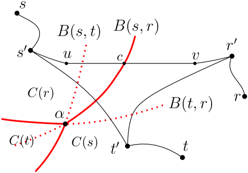
Figure 6: Illustrating $\mbox{$F\!V\!D$}(s,t,r)$, whose edges are depicted by thick (red) solid curves. The (red) dotted curves belong to bisectors but not on $\mbox{$F\!V\!D$}(s,t,r)$. The point $\alpha$ is the only vertex of $\mbox{$F\!V\!D$}(s,t,r)$ because it is equidistant from all three sites. The cells $C(s)$, $C(t)$, and $C(r)$ are ordered clockwise around $\alpha$, while $s$, $t$, and $r$ are ordered counterclockwise around the boundary of their geodesic hull, a contradiction.

The above proves that $\alpha$ is in $P_{1}$. Oh and Ahn [19] showed that $\overline{\alpha p_{t}}$ intersects $\overline{uv}$. The main proof idea is that if this were not the case, then a vertex of $P$ would be on a bisector of two of the three sites $s$, $t$, and $r$, contradicting with the general position assumption (see the proof of Lemma 3.6 [19] for the detailed analysis). This leads to the lemma statement (6), which further implies the lemma statement (5).

To simplify the notation, let $q=\beta(s,t)$. By definition, $q$ is on the bisector $B(s,t)$. As $\alpha$ is equidistant from $s$, $t$, and $r$, $\alpha$ is also on $B(s,t)$. Let $p_{st}$ be the middle point of $\pi(s,t)$. Hence, $p_{st}\in B(s,t)$.

We claim that $\alpha$ must be on $B(s,t)$ between $p_{st}$ and $q$ (e.g., see Fig. 7). Indeed, notice that $p_{st}$ is the point on $B(s,t)$ closest to $t$ and if we move a point $p$ from one end of $B(s,t)$ to the other end, $d(t,p)$ will first monotonically decrease until $p_{st}$ and then monotonically increase. By Observation 2, if we move a point $p$ along $B(s,t)$ from $q$ to $\alpha$, $d(t,p)$ will monotonically decrease. As such, $\alpha$ must be on $B(s,t)$ between $p_{st}$ and $q$.

We next argue that $q\in P_{1}$. Depending on whether $B(s,t)$ intersects $\overline{uv}$, there are two cases. If $B(s,t)$ does not intersect $\overline{uv}$, then as $\alpha\in B(s,t)$ and $\alpha\in P_{1}$, $B(s,t)$ is in $P_{1}$. Since $q\in B(s,t)$, $q\in P_{1}$ holds. If $B(s,t)$ intersects $\overline{uv}$, then since $\overline{uv}\subseteq\pi(s,r)$, by Observation 3, $B(s,t)$ intersects $\overline{uv}$ at a single point, denoted by $q_{st}$ (e.g., see Fig. 7). To prove $q\in P_{1}$, since $\alpha\in P_{1}$ and $\alpha$ is on $B(s,t)$ between $q$ and $p_{st}$, it suffices to show that $p_{st}\in P_{2}$. Indeed, since $B(s,t)$ intersects $\overline{uv}$ at $q_{st}$ and $\overline{uv}\subseteq\pi(s,r)$, by Observation 3, $B(s,t)$ does not intersect any other point of $\pi(s,r)$. Hence, $B(s,t)$ does not intersect $\pi(s,s^{\prime})\setminus\{s^{\prime}\}$, which is a subpath of $\pi(s,r)$ and does not contain any point of $\overline{uv}$. This implies that $p_{st}$ cannot be on $\pi(s,s^{\prime})\setminus\{s^{\prime}\}$ and thus is on $\pi(s^{\prime},t)$. Note that $s^{\prime}$ is in $P_{2}$. Since both $s^{\prime}$ and $t$ are in $P_{2}$, $\pi(s^{\prime},t)$ is in $P_{2}$. As such, $p_{st}\in P_{2}$.

The above proves that $q\in P_{1}$ and $\alpha$ is on $B(s,t)$ between $q$ and $p_{st}$. In the following, we proceed to prove that $\alpha\in\triangle(s,r,q)$.

Figure 7: Illustrating the relative positions of $\beta(s,t)$, $\alpha$, and $p_{st}$.

As $\alpha$ is on $B(s,t)$ between $q$ and $p_{st}$, $\alpha$ must be in the geodesic triangle $\triangle(s,t,q)$. Since $q\in B(s,t)$, due to the general position assumption, the incident edges of $q$ in $\pi(q,s)$ and $\pi(q,t)$ cannot be coincident [3]. This means that $q$ is the junction vertex of $\pi(q,s)$ and $\pi(q,t)$, and thus $q$ is an apex of $\triangle(s,t,q)$. Since $t\in P_{2}$ and $q\in P_{1}$, $\pi(q,t)$ must cross $\overline{uv}$ at a point $p$; e.g., see Fig. 5. Since both $\alpha$ and $q$ are in $P_{1}$, $\alpha$ is also in the geodesic triangle $\triangle(s,p,q)$ and $q$ is an apex of $\triangle(s,p,q)$. Further, since $p\in\overline{uv}\subseteq\pi(s,r)$, $\triangle(s,p,q)$ is a subset of $\triangle(s,r,q)$ and $q$ is also an apex of $\triangle(s,r,q)$. As such, we obtain that $\alpha\in\triangle(s,r,q)$. This proves the lemma statement (1).

The above also proves that $q$ is an apex of $\triangle(s,r,q)$. By definition, $u^{\prime}$ and $v^{\prime}$ are other two apexes of $\triangle(s,r,q)$. This proves the lemma statement (2). Since $\alpha\in\triangle(s,r,q)$, the lemma statements (3) and (4) obviously hold. $\Box$

In light of Lemma 5, we can apply the tentative prune-and-search technique [15] on the three pseudo-convex chains specified in the lemma in a similar way as before to compute $\alpha$ in $O(\log n)$ time.

We summarize our algorithm for this case. First, we compute the edge $\overline{uv}$, which can be done in $O(\log n)$ time using the GH data structure by Lemma 2. Second, we compute the junction vertex $t_{uv}$ of $\pi(t,u)$ and $\pi(t,v)$ in $O(\log n)$ time by the GH data structure [11]. Third, we apply the tentative prune-and-search technique on the three pseudo-convex chains as specified in Lemma 5, along with the binary search scheme in Lemma 2 on the chains, to compute $\alpha$ in $O(\log n)$ time.

Recall that the above algorithm is based on the assumption that $\alpha$ is a Voronoi vertex of $\mbox{$F\!V\!D$}(S)$. However, when we invoke the procedure during the geodesic sweeping algorithm we do not know whether the assumption is true. Therefore, as a final step, we add a validation procedure as follows. Suppose $\alpha$ is the point returned by the algorithm. First, we check whether $d(s,\alpha)=d(t,\alpha)=d(r,\alpha)$. If not, we return null. Otherwise, we further check whether $d(c^{*},\alpha)\leq\min\{d(c^{*},\beta(s,t)),d(c^{*},\beta(t,r))\}$. This is because the Voronoi vertex $\alpha$ is only useful if it is inside the current sweeping circle $C$, whose geodesic distance to $c^{*}$ is at most $\min\{d(c^{*},\beta(s,t)),d(c^{*},\beta(t,r))\}$ (because neither $\beta(s,t)$ nor $\beta(t,r)$ is in the interior of $C$). Hence, if $d(c^{*},\alpha)\leq\min\{d(c^{*},\beta(s,t)),d(c^{*},\beta(t,r))\}$, then we return $\alpha$; otherwise, we return null. This validation step takes $O(\log n)$ time by the GH data structure.

At least one of $u$ and $v$ is not a polygon vertex.

The above discusses the case where both $u$ and $v$ are polygon vertices. In the following, we consider the other case where at least one of them is not a polygon vertex, i.e., $u=s$ or/and $v=r$ (because all vertices of $\pi(s,r)$ except $s$ and $r$ are polygon vertices). In fact, this case is missed from the algorithm of Oh and Ahn [19] (see the proof of Lemma 3.6 [19]). It turns out that Lemma 5 still holds for this case and thus we can apply exactly the same algorithm as above. We prove the lemma below by reducing this case to the previous case where $u$ and $v$ are polygon vertices.

Lemma 6

Lemma 5 still holds when $u=s$ or/and $v=r$.

Proof: Without loss of generality, we assume that $v$ is not a polygon vertex and thus $v=r=r^{\prime}$. We extend $\overline{uv}$ in the direction from $u$ to $v$ until $\partial P$ at a point $v^{\prime}$ (e.g., see Fig. 8). If $u$ is also not a polygon vertex, then $u=s=s^{\prime}$ and we extend $\overline{uv}$ in the direction from $v$ to $u$ until $\partial P$ at a point $u^{\prime}$. If $u$ is a polygon vertex, we let $u^{\prime}=u$.

Let $P^{\prime}$ be the polygon obtained by adding $\overline{vv^{\prime}}$ and $\overline{uu^{\prime}}$ to $P$. So $P^{\prime}$ is a (weakly) simple polygon with $u$ and $v$ as two vertices. We claim that $B(s,t)$, $B(s,r)$, and $B(t,r)$ are still the bisectors of $s$, $t$, and $r$ in $P^{\prime}$. Before proving the claim, we proceed to prove the lemma with help of the claim. Due to the claim, since $u$ and $v$ are now both polygon vertices of $P^{\prime}$, we can apply literally the same argument as in the previous case. Indeed, the argument only relies on the properties of the three bisectors, e.g., $\alpha$ is their common intersection. Now that the three bisectors do not change from $P$ to $P^{\prime}$, the same argument still works. Thus, the lemma follows.

In the following, we prove the above claim. It is sufficient to show the following four properties: (1) $\overline{vv^{\prime}}\setminus\{v\}\cup\overline{uu^{\prime}}\setminus\{u\}$ does not intersect any of the three bisectors $B(s,t)$, $B(t,r)$, and $B(s,r)$; (2) $\overline{vv^{\prime}}\setminus\{v\}\cup\overline{uu^{\prime}}\setminus\{u\}$ does not intersect $\pi(s,p)$ for any point $p\in B(s,t)\cup B(s,r)$; (3) $\overline{vv^{\prime}}\setminus\{v\}\cup\overline{uu^{\prime}}\setminus\{u\}$ does not intersect $\pi(t,p)$ for any point $p\in B(s,t)\cup B(t,r)$; (4) $\overline{vv^{\prime}}\setminus\{v\}\cup\overline{uu^{\prime}}\setminus\{u\}$ does not intersect $\pi(r,p)$ for any point $p\in B(s,r)\cup B(t,r)$. Below we will prove the above four properties only for $\overline{vv^{\prime}}\setminus\{v\}$, as the proof for $\overline{uu^{\prime}}\setminus\{u\}$ is similar. We prove these properties in order.

Figure 8: Illustrating the proof of Lemma 6.

Property (1).

First of all, since $v^{\prime}$ is an extension of $\overline{uv}$, it holds that $\pi(s,v^{\prime})=\pi(s,v)\cup\overline{vv^{\prime}}$. Recall that $d(s,c)=d(c,r)>d(t,c)$ and $c\in\overline{uv}$. Assume to the contrary that $\overline{vv^{\prime}}$ intersects $B(s,t)$, say, at a point $z$. Then, $d(s,z)=d(s,c)+|\overline{cz}|$. On the other hand, by triangle inequality, $d(t,z)\leq d(t,c)+|\overline{cz}|$. Hence, we obtain $d(s,z)=d(s,c)+|\overline{cz}|>d(t,c)+|\overline{cz}|\geq d(t,z)$. However, since $z\in B(s,t)$, $d(s,z)=d(t,z)$, and thus contradiction occurs. This proves that $\overline{vv^{\prime}}$ does not intersect $B(s,t)$.

Because $\pi(s,v^{\prime})$ contains $\overline{rv^{\prime}}$, $d(s,p)>d(r,p)$ for any point $p\in\overline{vv^{\prime}}$. Therefore, $\overline{vv^{\prime}}\setminus\{v\}$ cannot intersect $B(s,r)$.

Next we prove the case for $B(t,r)$. Let $a$ be the anchor of $r$ in $\pi(t,r)$. Since $d(t,c)<d(r,c)=|\overline{cr}|$, the angle $\angle(a,r,c)$ must be smaller than $\pi/2$, and thus the angle $\angle(v^{\prime},r,a)$ is larger than $\pi/2$. Notice that $r$ is the junction vertex of $\pi(r,t)$ and $\pi(r,p)=\overline{rp}$ for any $p\in\overline{vv^{\prime}}\setminus\{v\}$. Since the angle $\angle(p,r,a)=\angle(v^{\prime},r,a)$ is larger than $\pi/2$, it must hold that $d(t,p)>d(r,p)$ [22] (see Corollary 2). This implies that $p$ cannot be on $B(t,r)$. Thus, $\overline{vv^{\prime}}\setminus\{v\}$ does not intersect $B(t,r)$.

This prove property (1).

Property (2).

We now prove property (2). Let $p$ be any point in $B(s,t)\cup B(s,r)$. Assume to the contrary that $\pi(s,p)$ contains a point $p^{\prime}\in\overline{vv^{\prime}}\setminus{v}$. Then, since $\pi(s,p^{\prime})$ contains $\pi(s,r)$, $\pi(s,p)$ contains $\pi(s,r)$ and thus contains $r$.

If $p\in B(s,r)$, then we immediately obtain contradiction as $\pi(s,p)$ cannot contain $r$.

Now consider the case $p\in B(s,t)$. Since $d(s,c)>d(t,c)$, there must be a point $p^{\prime\prime}\in\pi(s,c)$ such that $d(s,p^{\prime\prime})=d(t,p^{\prime\prime})$, i.e., $p^{\prime\prime}\in B(s,t)$. Since $\pi(s,p^{\prime\prime})\subseteq\pi(s,c)$ and $c\neq r$, $\pi(s,p^{\prime\prime})$ does not contain $r$. If $p=p^{\prime\prime}$, we obtain that $\pi(s,p)$ does not contain $r$, which incurs contradiction. Hence, $p\neq p^{\prime\prime}$. Thus, $\pi(s,p)$ intersects $B(s,t)$ at two different points $p$ and $p^{\prime\prime}$. But this is not possible due to Observation 3.

This proves property (2).

Property (3).

For property (3), let $p$ be any point in $B(s,t)\cup B(t,r)$. Assume to the contrary that $\pi(t,p)$ contains a point $p^{\prime}\in\overline{vv^{\prime}}\setminus\{v\}$.

We first discuss the case $p\in B(s,t)$. Consider the geodesic triangle $\triangle(s,t,p)$; e.g., see Fig. 9. Since $p\in B(s,t)$, $p$ must be an apex of $\triangle(s,t,p)$. Let $a$ be the junction vertex of $\pi(s,p)$ and $\pi(s,t)$ and let $b$ the junction vertex of $\pi(t,s)$ and $\pi(t,p)$. Hence, $a$ and $b$ are two apexes of $\triangle(s,t,p)$. By a similar argument as Observation 1, the middle point $p_{st}$ of $\pi(s,t)$ must be on $\pi(a,b)$, i.e., the side of $\triangle(s,t,p)$ opposite to $p$. Hence, the portion of $B(s,t)$ between $p$ and $p_{st}$, denoted by $B$, separates $\triangle(s,t,p)$ into two parts. As $\pi(t,p)=\pi(t,b)\cup\pi(b,p)$, $p^{\prime}$ is either in $\pi(t,b)$ or in $\pi(b,p)$.

Figure 9: Illustrating the pseudo-triangle $\triangle(s,t,p)$.

• If $p^{\prime}$ is in $\pi(t,b)$, then $p^{\prime}$ is in $\pi(s,t)$ as $\pi(t,b)$ is a subpath of $\pi(s,t)$. Therefore, $\pi(s,p^{\prime})$ is a subpath of $\pi(s,t)$. Recall that $\pi(s,r)\subseteq\pi(s,p^{\prime})$. We thus obtain that $\pi(s,r)$ is a subpath of $\pi(s,t)$. Since $c\in\pi(s,r)$, we obtain that $s$, $c$, $r$, and $t$ are all on $\pi(s,t)$ in this order. Hence, $d(c,r)\leq d(c,t)$, which incurs contradiction as $d(c,r)>d(c,t)$.

• If $p^{\prime}$ is in $\pi(b,p)$, then $\pi(s,p^{\prime})$ must intersect $B$, say, at a point $z$ (e.g., see Fig. 9). By Lemma 7, it holds that $d(s,z)\geq d(z,p^{\prime})$, and thus $d(s,z)\geq d(s,p^{\prime})/2$. Since $r\in\pi(s,p^{\prime})$, we have $d(s,z)\geq d(s,r)/2=d(s,c)$. This implies that $c\in\pi(s,z)$. Because $z\in B$, we have $d(s,c)\leq d(t,c)$. But this contradicts with the fact $d(s,c)>d(t,c)$.

The above obtains contradiction for the case $p\in B(s,t)$.

We next discuss the case $p\in B(t,r)$. The bisector $B(t,r)$ divides $P$ into two subpolygons; let $P_{t}$ be the one containing $t$ and let $P_{r}$ denote the one containing $r$. We assume that neither $P_{s}$ nor $P_{r}$ contains $B(t,r)$. As $p\in B(t,r)$, the entire path $\pi(t,p)$ is in $P_{t}\cup B(s,t)$. Since $p^{\prime}\in\overline{vv^{\prime}}\setminus\{v^{\prime}\}$, by a similar argument using the angle at $r$ as that for property (1), we can show that $d(t,p^{\prime})>d(r,p^{\prime})$. This implies that $p^{\prime}$ is in $P_{s}$. Therefore, $p^{\prime}$ cannot be in $\pi(s,p)$, a contradiction.

This proves property (3).

Property (4).

For property (4), assume to the contrary that $\pi(r,p)$ contains a point $p^{\prime}\in\overline{vv^{\prime}}\setminus\{v\}$.

We first discuss the case $p\in B(t,r)$. Let $a$ be the anchor of $r$ in $\pi(t,r)$. Recall that we have shown before that the angle $\angle(a,r,v^{\prime})$ is larger than $\pi/2$. Consider the geodesic triangle $\triangle(t,r,p)$.

• If $r$ is not an apex of $\triangle(t,r,p)$, then $\overline{ra}\in\pi(r,t)\cap\pi(r,p)$. Since $p^{\prime}\in\pi(r,p)$ and $p^{\prime}\not\in\overline{ra}$, we obtain that $\pi(r,p^{\prime})$ contains $a$. However, since $\angle(a,r,v^{\prime})>\pi/2$ and $p^{\prime}\in\overline{rv^{\prime}}$, $\pi(r,p^{\prime})=\overline{rp^{\prime}}$ does not contain $a$, a contradiction.

• If $r$ is an apex of $\triangle(t,r,p)$, then since $p\in B(t,r)$, the angle $\angle(a,r,b)$ must be smaller than $\pi/2$, where $b$ is the anchor of $r$ in $\pi(p,r)$. As $p^{\prime}\in\pi(r,p)$ and $\pi(r,p^{\prime})=\overline{rp^{\prime}}$, we obtain that $p^{\prime}\in\overline{rb}$ and thus $\angle(a,r,b)=\angle(a,r,p^{\prime})$. Hence, $\angle(a,r,p^{\prime})$ is smaller than $\pi/2$. However, $\angle(a,r,p^{\prime})=\angle(a,r,v^{\prime})$, which is larger than $\pi/2$. Thus we obtain contradiction.

We then discuss the case $p\in B(s,r)$. Note that $u$ is the anchor of $r$ in $\pi(s,r)$. Hence, the angle $\angle(u,r,v^{\prime})$ is equal to $\pi$, which is larger than $\pi/2$. Consequently, we can follow the same analysis as above to obtain contradiction.

This proves property (4).

The lemma thus follows. $\Box$

We finally prove the following technical lemma, which is needed in the proof of Lemma 6. The lemma, which establishes a very basic property of shortest paths in simple polygons, may be interesting in its own right.

Lemma 7

Let $s$ and $t$ be any two points in $P$ such that $B(s,t)$ does not contain any vertex of $P$. Suppose $p$ is a point in $B(s,t)$ and $p^{\prime}$ is a point in $\pi(t,p)$. Then, $\pi(s,p^{\prime})$ intersects $B(s,t)$ at a single point $z$ and $d(s,z)\geq d(z,p^{\prime})$ (in particular, $d(s,z)>d(z,p^{\prime})$ if $p^{\prime}\neq t$); e.g., see Fig. 9.

Proof: We first consider a special case where $p$ is the middle point $p_{st}$ of $\pi(s,t)$. Note that $p_{st}\in B(s,t)$. In this case, $z=p_{st}$ and $\pi(s,t)=\pi(s,z)\cup\pi(z,t)$. Hence, $\pi(s,p^{\prime})=\pi(s,z)\cup\pi(z,p^{\prime})$ and $d(s,z)=d(z,t)\geq d(z,p^{\prime})$ (and $d(s,z)=d(s,t)>d(z,p^{\prime})$ if $p^{\prime}\neq t$).

In the following we assume $p\neq p_{st}$. Consider the geodesic triangle $\triangle(s,t,p)$. Since $p\in B(s,t)$, $p$ is an apex of $\triangle(s,t,p)$. Let $a$ be the junction vertex of $\pi(s,t)$ and $\pi(s,p)$ and $b$ be the junction vertex of $\pi(t,s)$ and $\pi(t,p)$ (e.g., see Fig. 9). Hence, $a,b,p$ are the three apexes of $\triangle(s,t,p)$. In the following discussion we will use $\triangle(a,b,p)$ instead. By a similar argument as Observation 1, $p_{st}$ is in $\pi(a,b)$.

The bisector $B(s,t)$ partitions $P$ into two connected subpolygons $P_{s}$ and $P_{t}$ such that $P_{s}$ contains $s$ and $P_{t}$ contains $t$ [2]. We assume that neither $P_{s}$ nor $P_{t}$ contains $B(s,t)$. Since $p\in B(s,t)$, $\pi(s,p)\setminus\{p\}\subseteq P_{s}$ and $\pi(t,p)\setminus\{p\}\subseteq P_{t}$ [2]. This implies that $\pi(s,p^{\prime})$ intersects $B(s,t)$ at a single point $z$ because $s\in P_{s}$ and $p^{\prime}\not\in P_{s}$.

Since $p^{\prime}\in\pi(t,p)$, $p^{\prime}$ is either in $\pi(t,b)$ or in $\pi(b,p)\setminus\{b\}$. In the former case, $\pi(s,b)\subseteq\pi(s,p^{\prime})\subseteq\pi(s,t)$ and thus $z=p_{st}$. Hence, $d(s,z)=d(s,t)/2$. On the other hand, $\pi(z,p^{\prime})\subseteq\pi(z,t)$ and thus $d(z,p^{\prime})\leq d(z,t)=d(s,t)/2$ (and $d(z,p^{\prime})<d(z,t)$ if $p^{\prime}\neq t$). Therefore, we obtain that $d(s,z)\geq d(z,p^{\prime})$ (and $d(s,z)>d(z,p^{\prime})$ if $p^{\prime}\neq t$).

It remains to discuss the case $p^{\prime}\in\pi(b,p)\setminus\{b\}$. In this case, $p^{\prime}$ is a point on the boundary of $\triangle(a,b,p)$. Let $q$ be the anchor of $p^{\prime}$ in $\pi(s,p^{\prime})$. Because $p^{\prime}$ is on the boundary of $\triangle(a,b,p)$, $\pi(s,a)\subseteq\pi(s,p^{\prime})$ and $q$ is on the boundary of $\triangle(a,b,p)$. Since $p^{\prime}$ is in $\pi(b,p)$, which is the opposite side of the apex $a$, $q$ cannot be on $\pi(b,p)$ and thus must be on $\pi(a,p)\cup\pi(a,b)$. Note that $\pi(a,b)=\pi(a,p_{st})\cup\pi(p_{st},b)$.

Our goal is to prove $d(s,z)>d(z,p^{\prime})$. Assume to the contrary that $d(s,z)\leq d(z,p^{\prime})$. In the following we will obtain $d(s,p)>d(t,p)$, which incurs contradiction as $p\in B(s,t)$. Depending on whether $q$ is in $\pi(a,p)\cup\pi(a,p_{st})$ and $\pi(p_{st},b)\setminus\{p_{st}\}$, there are two cases. We first show that the latter case can be reduced to the former case.

Figure 10: Illustrating the proof of Lemma 7 for the case $q\in\pi(p_{st},b)\setminus\{p_{st}\}$.

If $q\in\pi(p_{st},b)\setminus\{p_{st}\}$, then $z=p_{st}$; e.g., see Fig. 10. Hence, $d(z,b)\leq d(t,z)=d(s,z)\leq d(z,p^{\prime})$. If we move a point $x$ on $\pi(b,p)$ from $b$ to $p$, then $d(s,x)$ is strictly convex [22] (see the proof of Lemma 1), and more precisely, $d(s,x)$ first strictly decreases until a point $x^{*}$ and then strictly increases. We claim that $x^{*}\in\pi(b,p^{\prime})$. Indeed, assume to the contrary that $x^{*}\in\pi(p^{\prime},p)$. Then, we can obtain $d(s,p^{\prime})<d(s,b)$. Because both $\pi(s,p^{\prime})$ and $\pi(s,b)$ contain $z$, we derive that $d(z,p^{\prime})<d(z,b)$, which contradicts with $d(z,p^{\prime})\geq d(z,b)$. Due to the above claim, as we move $x$ from $p^{\prime}$ to $p$ along $\pi(p^{\prime},p)$, $\pi(s,x)$ will strictly increase. We stop moving $x$ when $\overline{xx^{\prime}}$ contains $p_{st}$ (e.g., see Fig. 10), where $x^{\prime}$ is the anchor of $x$ in $\pi(s,x)$. Note that such a moment must exist as $\pi(s,p)$ does not contain $p_{st}$. As $p_{st}\in\pi(s,p^{\prime})$, $z$ is still $p_{st}$. Since $d(s,x)>d(s,p^{\prime})$ and both $\pi(s,x)$ and $\pi(s,p^{\prime})$ contain $z$, we can obtain that $d(z,p^{\prime})<d(z,x)$. As $d(s,z)\leq d(z,p^{\prime})$, we deduce that $d(s,z)\leq d(z,x)$. Now we obtain an instance of the first case (i.e., $q\in\pi(a,p)\cup\pi(a,p_{st})$) because $x^{\prime}\in\pi(a,p_{st})$, i.e., we can consider $x$ as a new point $p^{\prime}$ and obtain contradiction by using the analysis given below for the first case.

Figure 11: Illustrating the proof of Lemma 7: (a) $q\in\pi(a,p)$; (b) $q\in\pi(a,p_{st})$.

In the following we consider the case where $q\in\pi(a,p)\cup\pi(a,p_{st})$; e.g., see Fig. 11. In this case, $\overline{qp^{\prime}}$ intersects $B(s,t)$ at $z$ and thus $d(z,p^{\prime})=\overline{zp^{\prime}}$. There are two subcases depending on whether $q\in\pi(a,p)$ or $q\in\pi(a,p_{st})$. For each case, we will construct a geodesic triangle $\triangle(a^{\prime},b^{\prime},p)$ (which may not be in $P$) with the following properties: (1) $a^{\prime}$, $b^{\prime}$, and $p$ are its three apexes; (2) the length of the side of $\triangle(a^{\prime},b^{\prime},p)$ connecting $a^{\prime}$ and $p$, denoted by $l(a^{\prime},p)$, is at most $d(s,p)$; (3) the length of the side of $\triangle(a^{\prime},b^{\prime},p)$ connecting $b^{\prime}$ and $p$, denoted by $l(b^{\prime},p)$, is equal to $d(b,p)$; (4) the angle at $b^{\prime}$ formed by its two incident edges of $\triangle(a^{\prime},b^{\prime},p)$ is at least $\pi/2$. These properties together lead to $d(s,p)>d(t,p)$. Indeed, due to property (4), it holds that $l(b^{\prime},p)<l(a^{\prime},p)$ [22] (see Corollary 2). Combining with properties (2) and (3), we have $d(t,p)=l(b^{\prime},p)<l(a^{\prime},p)\leq d(s,p)$. This incurs contradiction since $d(t,p)=d(s,p)$.

Figure 12: Illustrating the definitions of $a^{\prime}$, $b^{\prime}$, $w$, and $z^{\prime}$ in the proof of Lemma 7.

The first subcase $q\in\pi(a,p)$.

We begin with the subcase $q\in\pi(a,p)$; e.g., see Fig. 11(a). We extend $\overline{p^{\prime}q}$ along the direction from $p^{\prime}$ to $q$ until a point $a^{\prime}$ such that $|\overline{qa^{\prime}}|=d(s,q)$; note that $\overline{qa^{\prime}}$ may not be in $P$. Refer to Fig. 12. Note that $\pi(p,q)\cup\overline{qa^{\prime}}$ is still a convex chain and its length $l(a^{\prime},p)$ is equal to $|\overline{qa^{\prime}}|+d(q,p)=d(s,q)+d(q,p)=d(s,p)$. Let $p^{\prime\prime}$ be the vertex of $\pi(p^{\prime},p)$ incident to $p^{\prime}$. We extend $\overline{p^{\prime\prime}p^{\prime}}$ along the direction from $p^{\prime\prime}$ to $p^{\prime}$ until a point $b^{\prime}$ such that $|\overline{p^{\prime}b^{\prime}}|=d(t,p^{\prime})$. Note that $\pi(p,p^{\prime})\cup\overline{p^{\prime}b^{\prime}}$ is still a convex chain and its length $l(b^{\prime},p)$ is equal to $|\overline{p^{\prime}b^{\prime}}|+d(p^{\prime},p)=d(t,p^{\prime})+d(p^{\prime},p)=d(t,p)$. In the following we show that the angle $\angle(p^{\prime},b^{\prime},a^{\prime})$ is at least $\pi/2$; this will prove all four properties described above for the geodesic triangle $\triangle(a^{\prime},b^{\prime},p)$.

We claim that $|\overline{zb^{\prime}}|\leq d(z,t)$. Before proving the claim, we first show $\angle(p^{\prime},b^{\prime},a^{\prime})\geq\pi/2$ by using the claim. Indeed, notice that $|\overline{za^{\prime}}|=|\overline{zq}|+|\overline{qa^{\prime}}|=|\overline{zq}|+d(s,q)=d(s,z)$. As $z\in B(s,t)$, $d(s,z)=d(t,z)$. Hence, $|\overline{za^{\prime}}|\geq|\overline{zb^{\prime}}|$. Recall that $d(s,z)\leq d(z,p^{\prime})=|\overline{zp^{\prime}}|$. Therefore, we have $|\overline{zp^{\prime}}|\geq|\overline{za^{\prime}}|\geq|\overline{zb^{\prime}}|$. If we draw a circle centered at $z$ with radius equal to $|\overline{za^{\prime}}|$, then $a^{\prime}$ is on the circle, $b^{\prime}$ is inside or on the circle, and $p^{\prime}$ is outside or on the circle. Since $\overline{a^{\prime}p^{\prime}}$ contains a diameter of the circle, we obtain that $\angle(p^{\prime},b^{\prime},a^{\prime})\geq\pi/2$.

We proceed to prove the claim $|\overline{zb^{\prime}}|\leq d(z,t)$. Notice that $\overline{p^{\prime}b^{\prime}}$ must intersect $\pi(z,b)$. Indeed, unless $\overline{p^{\prime}b^{\prime}}$ contains $b$ (in which case it is vacuously true that $\overline{p^{\prime}b^{\prime}}$ intersects $\pi(z,b)$), as $\overline{p^{\prime}b^{\prime}}$ is tangent to $\pi(b,p)$ at $p^{\prime}$, if we move on $\overline{p^{\prime}b^{\prime}}$ from $p^{\prime}$ towards $b^{\prime}$, we will enter the interior of $\triangle(a,b,p)$ and let $w$ be the first point on the boundary of $\triangle(a,b,p)$ we meet during the above movement after $p^{\prime}$ (i.e., we will go outside $\triangle(a,b,p)$ after $w$; e.g., see Fig. 12). Then, $\overline{p^{\prime}w}$ separates $z$ and $b$ on its two sides, and thus $\overline{p^{\prime}w}$ must intersect $\pi(z,b)$, say, at a point $z^{\prime}$. We next prove $|\overline{z^{\prime}b^{\prime}}|\leq d(z^{\prime},t)$. Indeed, $d(t,p^{\prime})=|\overline{p^{\prime}b^{\prime}}|=|\overline{p^{\prime}z^{\prime}}|+|\overline{z^{\prime}b^{\prime}}|$. On the other hand, by triangle inequality, $d(t,p^{\prime})\leq|\overline{p^{\prime}z^{\prime}}|+d(z^{\prime},t)$. Hence, we obtain $|\overline{z^{\prime}b^{\prime}}|\leq d(z^{\prime},t)$. Consequently, by triangle inequality, $|\overline{zb^{\prime}}|\leq d(z,z^{\prime})+|\overline{z^{\prime}b^{\prime}}|\leq d(z,z^{\prime})+d(z^{\prime},t)=d(z,t)$. This proves the claim.

The above proves the first subcase $q\in\pi(a,p)$.

The second subcase $q\in\pi(a,p_{st})$.

We next discuss the subcase $q\in\pi(a,p_{st})$; e.g., see Fig. 11(b). The analysis is somewhat similar. First of all, we define $b^{\prime}$ in the same way as above; by the same argument, we have: (1) $\pi(p,p^{\prime})\cup\overline{p^{\prime}b^{\prime}}$ is a convex chain and its length is equal to $d(p,b)$; (2) $|\overline{zb^{\prime}}|\leq d(z,t)$.

Figure 13: Illustrating the definitions of $a^{\prime}$, $b^{\prime}$, and $q^{\prime}$ in the proof of Lemma 7.

The point $a^{\prime}$ is now defined in a slightly different way. Refer to Fig. 13. We extend $\overline{p^{\prime}q}$ from $p^{\prime}$ to $q$ until a point $a^{\prime}$ that satisfies the following two conditions: (1) $|\overline{qa^{\prime}}|\geq d(s,q)$; (2) $\overline{p^{\prime}a^{\prime}}$ intersects $\pi(a,p)$, say, at a point $q^{\prime}$ (this is possible as $\overline{p^{\prime}q}$ is tangent to $\pi(a,p_{st})$ at $q$). Note that $a^{\prime}=q^{\prime}$ if and only if $|\overline{qq^{\prime}}|\geq d(s,q)$. Also note that $|\overline{qa^{\prime}}|=d(s,q)$ if $a^{\prime}\neq q^{\prime}$. Next we prove the four properties of the geodesic triangle $\triangle(a^{\prime},b^{\prime},p)$.

First of all, notice that $|\overline{a^{\prime}z}|=|\overline{a^{\prime}q}|+|\overline{qz}|\geq d(s,q)+|\overline{qz}|=d(s,z)$. Recall that $|\overline{zb^{\prime}}|\leq d(t,z)=d(s,z)$ and $d(s,z)\leq|\overline{zp^{\prime}}|$. By a similar argument as before for the first subcase, the angle $\angle(a^{\prime},b^{\prime},p^{\prime})$ is at least $\pi/2$. By the definitions of $a^{\prime}$ and $q^{\prime}$, $\pi(p,q^{\prime})\cup\overline{q^{\prime}a^{\prime}}$ is a convex chain and we will show below that its length $l(a^{\prime},p)$ is at most $d(s,p)$, which will prove all four properties of $\triangle(a^{\prime},b^{\prime},p)$.

To prove $l(a^{\prime},p)\leq d(s,p)$, as $l(a^{\prime},p)=|\overline{a^{\prime}q^{\prime}}|+d(q^{\prime},p)$ and $d(s,p)=d(s,q^{\prime})+d(q^{\prime},p)$, it is sufficient to prove $|\overline{a^{\prime}q^{\prime}}|\leq d(s,q^{\prime})$. If $a^{\prime}=q^{\prime}$, this is obviously true. We thus assume $a^{\prime}\neq q^{\prime}$. Then, $|\overline{qq^{\prime}}|<|\overline{qa^{\prime}}|=d(s,q)$. Hence, $d(s,p^{\prime})=d(s,q)+|\overline{qp^{\prime}}|=|\overline{qa^{\prime}}|+|\overline{qp^{\prime}}|=|\overline{a^{\prime}p^{\prime}}|=|\overline{a^{\prime}q^{\prime}}|+|\overline{q^{\prime}p^{\prime}}|$. On the other hand, by triangle inequality, $d(s,p^{\prime})\leq d(s,q^{\prime})+|\overline{q^{\prime}p^{\prime}}|$. Therefore, we obtain $|\overline{a^{\prime}q^{\prime}}|\leq d(s,q^{\prime})$.

The above proves the second subcase $q\in\pi(a,p_{st})$.

The lemma thus follows. $\Box$

4.2.2 The case $c\in\pi(s,s^{\prime})\setminus\{s^{\prime}\}$

We now consider the case $c\in\pi(s,s^{\prime})\setminus\{s^{\prime}\}$. For this case, Oh and Ahn [19] (see the proof of Lemma 3.6 [19]) claimed that $\alpha$ does not exist. However, this is not correct; see Fig. 14 for a counterexample.

Figure 14: Illustrating an example where $\alpha$ exists when $c\in\pi(s,s^{\prime})\setminus\{s^{\prime}\}$. The apexes of the geodesic triangle $\triangle(s,r,t)$ are $s^{\prime}$, $r^{\prime}=r$, and $t^{\prime}=t$. $|\overline{s^{\prime}t}|<|\overline{s^{\prime}r}|$. $c$ is the middle point of $\pi(s,r)=\overline{ss^{\prime}}\cup\overline{s^{\prime}r}$. However, one can verify (e.g., by a ruler) that $q$ is equidistant to $s$, $r$, and $t$, and thus $\alpha=q$ exists.

Let $v$ be the vertex incident to $s^{\prime}$ in $\pi(s^{\prime},r^{\prime})$. To make the notation consistent with the previous subcase, we let $u=s^{\prime}$. We have the following lemma (e.g., see Fig. 15), which is literally the same as Lemma 5 (the proof is also somewhat similar).

Figure 15: Illustrating Lemma 8. In this example, $v^{\prime}=v$.

Lemma 8

1. $\alpha$ must be in the geodesic triangle $\triangle(s,r,\beta(s,t))$.

2. The apexes of $\triangle(s,r,\beta(s,t))$ are $u^{\prime}$, $v^{\prime}$, and $\beta(s,t)$, where $u^{\prime}$ (resp., $v^{\prime}$) is the junction vertex of and $\pi(s,r)$ and $\pi(s,\beta(s,t))$ (resp., $\pi(r,\beta(s,t))$) (in Fig. 15, $v^{\prime}=v$).

3. $p_{s}$ must be on the pseudo-convex chain $\pi(u^{\prime},\beta(s,t))\cup\pi(u^{\prime},v^{\prime})$ and $\overline{\alpha p_{s}}$ is tangent to the chain.

4. $p_{r}$ must be on the pseudo-convex chain $\pi(v^{\prime},\beta(s,t))\cup\pi(v^{\prime},u^{\prime})$ and $\overline{\alpha p_{r}}$ is tangent to the chain.

5. $p_{t}$ must be on the pseudo-convex chain $\pi(t_{uv},u)\cup\pi(t_{uv},v)$ and $\overline{\alpha p_{t}}$ is tangent to the chain, where $t_{uv}$ is the junction vertex of $\pi(t,u)$ and $\pi(t,v)$.

6. $\overline{\alpha p_{t}}$ intersects $\overline{uv}$.

Proof: As $c\in\pi(s,s^{\prime})\setminus\{s^{\prime}\}$ and $u=s^{\prime}$, $u$ cannot be $s$ and thus must be a polygon vertex. But $v$ can be either a polygon vertex or the site $r$. We assume that $v$ is a polygon vertex since the other case can be reduced to this case by the same technique as in the proof of Lemma 6.

As both $u$ and $v$ are polygon vertices, $\overline{uv}$ divides $P$ into two sub-polygons; one of them, denoted by $P_{1}$, does not contain $t$ and we use $P_{2}$ to denote the other one. Let $P^{\prime}$ be the one of $P_{1}$ and $P_{2}$ that contains $s$. We will argue later that $P^{\prime}$ must be $P_{1}$.

We first show that the bisector $B(s,t)$ is in $P^{\prime}$. Recall that $p_{st}$ is the middle point of $B(s,t)$. Since $c\in\pi(s,s^{\prime})\setminus\{s^{\prime}\}$ and $d(s,c)=d(r,c)>d(c,t)$, $d(s,t)=d(s,c)+d(t,c)<d(s,c)+d(c,r)=d(s,r)$. Hence $d(s,p_{st})=d(s,t)/2<d(s,r)/2=d(s,c)$. Thus, $p_{st}\in\pi(s,c)\setminus\{c\}$. Note that $\pi(s,c)$ is in $P^{\prime}$ since $\pi(s,c)\subseteq\pi(s,u)$ and $\pi(s,u)\in P^{\prime}$ (the latter holds because both $s$ and $u$ are in $P^{\prime}$). Therefore, $p_{st}\in P^{\prime}$. Further, as $p_{st}\in\pi(s,c)\subseteq\pi(s,u)\setminus\{u\}$, $p_{st}\not\in\overline{uv}$. Since $p_{st}\in\pi(s,r)$, $B(s,t)$ does not intersect $\pi(s,r)$ other than $p_{st}$ by Observation 3. As $\overline{uv}\subseteq\pi(s,r)$, we obtain that $B(s,t)$ does not intersect $\overline{uv}$. Because $p_{st}$ is in $B(s,t)\cap P^{\prime}$ and $B(s,t)$ does not intersect $\overline{uv}$, $B(s,t)$ must be in $P^{\prime}$.

Since $c\in\pi(s,s^{\prime})\setminus\{s^{\prime}\}$ and $c\in B(s,r)$, $B(s,r)$ is also in $P^{\prime}$ by following the analysis similar to the above. As $\alpha$ is equidistant from $s$, $t$, and $r$, $\alpha$ is on both $B(s,t)$ and $B(s,r)$. Therefore, $\alpha$ is in $P^{\prime}$.

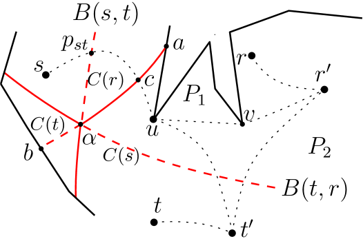
Figure 16: Illustrating $\mbox{$F\!V\!D$}(s,t,r)$, whose edges are depicted by thick (red) solid curves. The black solid segments are part of the boundary of $P$. The (red) dotted curves belong to bisectors but not on $\mbox{$F\!V\!D$}(s,t,r)$. The red curve connecting $a$ and $b$ is $B(s,r)$; the portion between $c$ and $a$ (resp., $b$) is $B_{1}(s,r)$ (resp., $B_{2}(s,r)$). The point $\alpha$ is the only vertex of $\mbox{$F\!V\!D$}(s,t,r)$ because it is equidistant from all three sites. The cells $C(s)$, $C(t)$, and $C(r)$ are ordered clockwise around $\alpha$, while $s$, $t$, and $r$ are ordered counterclockwise around the boundary of their geodesic hull, a contradiction.

We next argue that $P^{\prime}$ must be $P_{1}$. We assume that $s$, $t$, $r$ are ordered counterclockwise around the boundary of their geodesic hull (e.g., see Fig. 15). Assume to the contrary that $P^{\prime}$ is $P_{2}$ (e.g., see Fig. 16). The point $c$ divides $B(s,r)$ into two portions, one going above $\pi(s,r)$ and the other going below $\pi(s,r)$ (we intuitively assume that $\pi(s,r)$ from $s$ to $r$ goes “horizontally” from left to right); let $B_{1}(s,r)$ (resp., $B_{2}(s,r)$) be the first (resp., second) portion (e.g., see Fig. 16, where the red curve between $c$ and $a$ is $B_{1}(s,r)$ and the red curve between $c$ and $b$ is $B_{2}(s,r)$). Since $P^{\prime}$ is $P_{2}$, the two polygon edges of $P$ incident to $u$ must be from the “above” of $\pi(s,r)$. Hence, for any point $p\in B_{1}(s,r)$, both shortest paths $\pi(s,p)$ and $\pi(t,p)$ must contain $u$. Thus, $d(r,p)=d(r,u)+d(u,p)$ and $d(t,p)=d(t,u)+d(u,p)$. Since $d(r,c)>d(t,c)$ and both $\pi(r,c)$ and $\pi(t,c)$ contain $u$, $d(r,u)>d(t,u)$ holds. Therefore, $d(r,p)>d(t,p)$. This implies that no point on $B_{1}(s,r)$ is equidistant from $r$ and $t$, and thus $B_{1}(s,r)$ does not contain $\alpha$. As $\alpha\in B(s,r)$, we have $\alpha\in B_{2}(s,r)$. Consider the farthest Voronoi diagram $\mbox{$F\!V\!D$}(s,t,r)$ of the three sites $s,t,r$ only (without considering other sites of $S$). Let $C(p)$ be the cell of $p\in\{s,t,r\}$ in the diagram. As $d(c,s)=d(c,r)>d(c,t)$, $c$ belongs to the common boundary of $C(s)$ and $C(r)$, i.e., $c$ is on an edge of $\mbox{$F\!V\!D$}(s,t,r)$. The point $\alpha$ divides $B(s,r)$ into two portions, one of which contains $c$. The above implies that the portion of $B(s,r)$ containing $c$ is an edge of $\mbox{$F\!V\!D$}(s,t,r)$ (e.g., see Fig. 16). Recall that $p_{st}\in\pi(s,c)\setminus\{c\}$. Since $\pi(s,c)\subset\pi(s,r)$ and $c$ is the middle point of $\pi(s,r)$, we obtain that $d(s,p_{st})=d(t,p_{st})<d(r,p_{st})$, implying that $p_{st}\in C(r)$. The point $\alpha$ partitions $B(s,t)$ into two portions, one of which contains $p_{st}$; since $p_{st}\in C(r)$, the portion of $B(s,t)$ containing $p_{st}$ is not an edge of $F(s,t,r)$. Then, one can verify that the three cells $C(s)$, $C(t)$, and $C(r)$ in $\mbox{$F\!V\!D$}(s,t,r)$ are ordered clockwise along the boundary of $P$ (e.g., see Fig. 16). According to Aronov [3], $s$, $t$, and $r$ should also be ordered clockwise around the boundary of their geodesic hull. But this contradicts with the fact that $s$, $t$, and $r$ are ordered counterclockwise around the boundary of their geodesic hull.

The above proves that $P^{\prime}$ is $P_{1}$. Since $B(s,t)\in P^{\prime}$ and $\alpha\in B(s,t)$, we obtain that $\alpha\in P_{1}$.

We next argue that $\alpha$ must be in the geodesic triangle $\triangle(s,r,\beta(s,t))$. The argument is similar to the proof of Lemma 5, so we briefly discuss it. To simplify the notation, let $q=\beta(s,t)$. Since $q\in B(s,t)$ and $B(s,t)\in P_{1}$, $q$ is in $P_{1}$. By the same analysis as in the proof of Lemma 5, $\alpha$ is on $B(s,t)$ between $p_{st}$ and $q$ (e.g., see Fig. 15), and thus $\alpha$ is in the geodesic triangle $\triangle(s,t,q)$ and $q$ is an apex of $\triangle(s,t,q)$. Since $t\in P_{2}$ and $q\in P_{1}$, $\pi(q,t)$ must cross $\overline{uv}$ at a point $p$, and thus $\alpha$ is also in $\triangle(s,p,q)$ and $q$ is an apex of $\triangle(s,p,q)$. Further, since $p\in\overline{uv}\subseteq\pi(s,r)$, $\alpha$ is in $\triangle(s,r,q)$ and $q$ is an apex of $\triangle(s,r,q)$.

This proves the lemma statements (1) and (2). The lemma statements (3) and (4) also immediately follow.

Finally, we argue that $\overline{\alpha p_{t}}$ intersects $\overline{uv}$. Assume to the contrary that this is not true. Since $\alpha\in P_{1}$ and $t\in P_{2}$, $\pi(\alpha,t)$ must cross $\overline{uv}$ at a point $z$. As $\overline{\alpha p_{t}}$ does not intersect $\overline{uv}$, $p_{t}$ must be a polygon vertex in $\pi(\alpha,z)$, which is subpath of $\pi(\alpha,t)$. As $z\in\overline{uv}\subseteq\pi(s,r)$, $\pi(\alpha,z)$ must be “between” $\pi(\alpha,s)$ and $\pi(\alpha,r)$. Since no two paths of $\pi(\alpha,s)$, $\pi(\alpha,z)$, and $\pi(\alpha,r)$ cross each other and $P$ is a simple polygon, $p_{t}$ must be in either $\pi(\alpha,s)$ and $\pi(\alpha,r)$. As $p_{t}\in\pi(\alpha,t)$ and $\alpha$ is equidistant from $s$, $t$, and $r$, $p_{t}$ is on the bisector between $t$ and one of $s$ and $r$. This contradicts with our general position assumption since $p_{t}$ is a vertex of $P$.

The above proves that $\overline{\alpha p_{t}}$ intersects $\overline{uv}$, i.e., the lemma statement (6), which also leads to the lemma statement (5). $\Box$

Due to the preceding lemma, our algorithm works as follows. First, we compute the vertices $u^{\prime}$, $v^{\prime}$, and $t_{uv}$, which can be done in $O(\log n)$ time by the GH data structure. Then we apply the tentative prune-and-search technique [15] on the three pseudo-convex chains specified in the lemma in a similar way as before to compute $\alpha$ in $O(\log n)$ time. Finally, we validate $\alpha$ in $O(\log n)$ time in a similar way as before. The overall time of the algorithm is $O(\log n)$. Lemma 1 is thus proved.

Remark.

As discussed above, there are two mistakes in the algorithm of Oh and Ahn [19] (Lemma 3.6): (1) In the subcase $c\in\pi(s^{\prime},r^{\prime})$, the case where not both $u$ and $v$ are polygon vertices is missed; (2) in the subcase $c\not\in\pi(s^{\prime},r^{\prime})$, they erroneously claimed that $\alpha$ does not exist. Both mistakes can be corrected with our new results. Indeed, in both cases we have proved that $\overline{\alpha p_{t}}$ intersects $\overline{uv}$. With this critical property, their algorithm of Lemma 3.6 [19] (which was originally designed for the case where $c\in\pi(s^{\prime},r^{\prime})$ and both $u$ and $v$ are polygon vertices) can be applied to compute $\alpha$ in $O(\log^{2}n)$ time. In this way, Lemma 3.6 of [19] is remedied and thus all other results of [19] that rely on Lemma 3.6 are not affected.

References

- [1] H.-K. Ahn, L. Barba, P. Bose, J.-L. De Carufel, M. Korman, and E. Oh. A linear-time algorithm for the geodesic center of a simple polygon. Discrete and Computational Geometry, 56:836–859, 2016.
- [2] B. Aronov. On the geodesic Voronoi diagram of point sites in a simple polygon. Algorithmica, 4:109–140, 1989.
- [3] B. Aronov, S. Fortune, and G. Wilfong. The furthest-site geodesic Voronoi diagram. Discrete and Computational Geometry, 9:217–255, 1993.
- [4] T. Asano and G. Toussaint. Computing the geodesic center of a simple polygon. Technical Report SOCS-85.32, McGill University, Montreal, Canada, 1985.
- [5] S.W. Bae and K.Y. Chwa. The geodesic farthest-site Voronoi diagram in a polygonal domain with holes. In Proceedings of the 25th ACM Symposium on Computational Geometry (SoCG), pages 198–207, 2009.
- [6] S.W. Bae, M. Korman, and Y. Okamoto. The geodesic diameter of polygonal domains. Discrete and Computational Geometry, 50:306–329, 2013.
- [7] S.W. Bae, M. Korman, and Y. Okamoto. Computing the geodesic centers of a polygonal domain. Computational Geometry: Theory and Applications, 77:3–9, 2019.
- [8] L. Barba. Optimal algorithm for geodesic farthest-point Voronoi diagrams. In Proceedings of the 35th International Symposium on Computational Geometry (SoCG), pages 12:1–12:14, 2019.
- [9] B. Chazelle. A theorem on polygon cutting with applications. In Proceedings of the 23rd Annual Symposium on Foundations of Computer Science (FOCS), pages 339–349, 1982.
- [10] B. Chazelle, H. Edelsbrunner, M. Grigni, L. Guibas, J. Hershberger, M. Sharir, and J. Snoeyink. Ray shooting in polygons using geodesic triangulations. Algorithmica, 12(1):54–68, 1994.
- [11] L.J. Guibas and J. Hershberger. Optimal shortest path queries in a simple polygon. Journal of Computer and System Sciences, 39(2):126–152, 1989.
- [12] J. Hershberger. A new data structure for shortest path queries in a simple polygon. Information Processing Letters, 38(5):231–235, 1991.
- [13] J. Hershberger and S. Suri. Matrix searching with the shortest-path metric. SIAM Journal on Computing, 26(6):1612–1634, 1997.
- [14] J. Hershberger and S. Suri. An optimal algorithm for Euclidean shortest paths in the plane. SIAM Journal on Computing, 28(6):2215–2256, 1999.
- [15] D. Kirkpatrick and J. Snoeyink. Tentative prune-and-search for computing fixed-points with applications to geometric computation. Fundamenta Informaticae, 22(4):353–370, 1995.
- [16] C.-H. Liu. A nearly optimal algorithm for the geodesic Voronoi diagram of points in a simple polygon. Algorithmica, 82:915–937, 2020.
- [17] J.S.B. Mitchell. Geometric shortest paths and network optimization, in Handbook of Computational Geometry, J.-R Sack and J. Urrutia (eds.), pages 633–702. Elsevier, Amsterdam, the Netherlands, 2000.
- [18] E. Oh. Optimal algorithm for geodesic nearest-point Voronoi diagrams in simple polygons. In Proceedings of the 20th Annual ACM-SIAM Symposium on Discrete Algorithms (SODA), pages 391–409, 2019.
- [19] E. Oh and H.-K. Ahn. Voronoi diagrams for a moderate-sized point-set in a simple polygon. Discrete and Computational Geometry, 63:418–454, 2020.
- [20] E. Oh, L. Barba, and H.-K. Ahn. The geodesic farthest-point Voronoi diagram in a simple polygon. Algorithmica, 82:1434–1473, 2020.
- [21] E. Papadopoulou and D.T. Lee. A new approach for the geodesic Voronoi diagram of points in a simple polygon and other restricted polygonal domains. Algorithmica, 20:319–352, 1998.
- [22] R. Pollack, M. Sharir, and G. Rote. Computing the geodesic center of a simple polygon. Discrete and Computational Geometry, 4(1):611–626, 1989.
- [23] F.P. Preparata and M.I. Shamos. Computational Geometry. Springer-Verlag, New York, 1985.
- [24] S. Suri. Computing geodesic furthest neighbors in simple polygons. Journal of Computer and System Sciences, 39:220–235, 1989.
- [25] G. Toussaint. Computing geodesic properties inside a simple polygon. Technical report, McGill University, Montreal, Canada, 1989.
- [26] H. Wang. On the geodesic centers of polygonal domains. Journal of Computational Geometry, 9:131–190, 2018.